Embed Size (px)
Citation preview

Supervised and unsupervised analysis of gene expression data
Bing Zhang
Department of Biomedical Informatics
Vanderbilt University

Overall workflow of gene expression studies
Microarray
Biological question
Experimental design
Image analysis
Data Analysis
HypothesisExperimental
validation
Reads mapping
RNA-Seq
2
Peptide/protein ID
Shotgun proteomics
Spectral counts;Peak intensities
Read countsSignal intensities

Data matrixG
enes
Samples
3
Spectral counts;Peak intensities
Read countsSignal intensities

Three major goals of gene expression studies
Differential expression (supervised analysis) Input: gene expression data, class label of the samples
Output: differentially expressed genes
e.g. disease biomarker discovery
Clustering (unsupervised analysis) Input: gene expression data
Output: groups of similar samples or genes
e.g. disease subtype identification
Classification (machine learning) Input: gene expression data, class label of the samples (training data)
Output: prediction model
e.g. disease diagnosis and prognosis
4

Data preprocessing I: missing value imputation
Replace with zeros Replace all missing values with 0
Replace with row averages Replace missing values with mean of available values in each row
(gene)
KNN imputation Estimate missing values via the K-nearest neighbors analysis
sample1 sample2 sample3 sample4 sample5 sample6gene1 1.3 1 1.1 1.2 2.4 1.5gene2 1.2 1.4 1.3 1.5 3.5 3.6gene3 2.3 2.1 NA 2.4 2.3 3.4gene4 3.5 3.3 3.6 3 0.8 1.8gene5 1.2 1.3 1.4 1.5 3.6 2.2
5

Data preprocessing II: normalization
To remove systematic variations and make experiments comparable
Use some control or housekeeping genes that you would expect to have the same expression level across all experiments
Use spike-in controls
Equalize the mean values for all experiments (Global normalization)
Match data distributions for all experiments (Quantile normalization)
No normalization Global normalization Quantile normalization
6

Data preprocessing III: transformation
To make the data more closely meet the assumptions of a statistical inference procedure
log transformation to improve normality
7
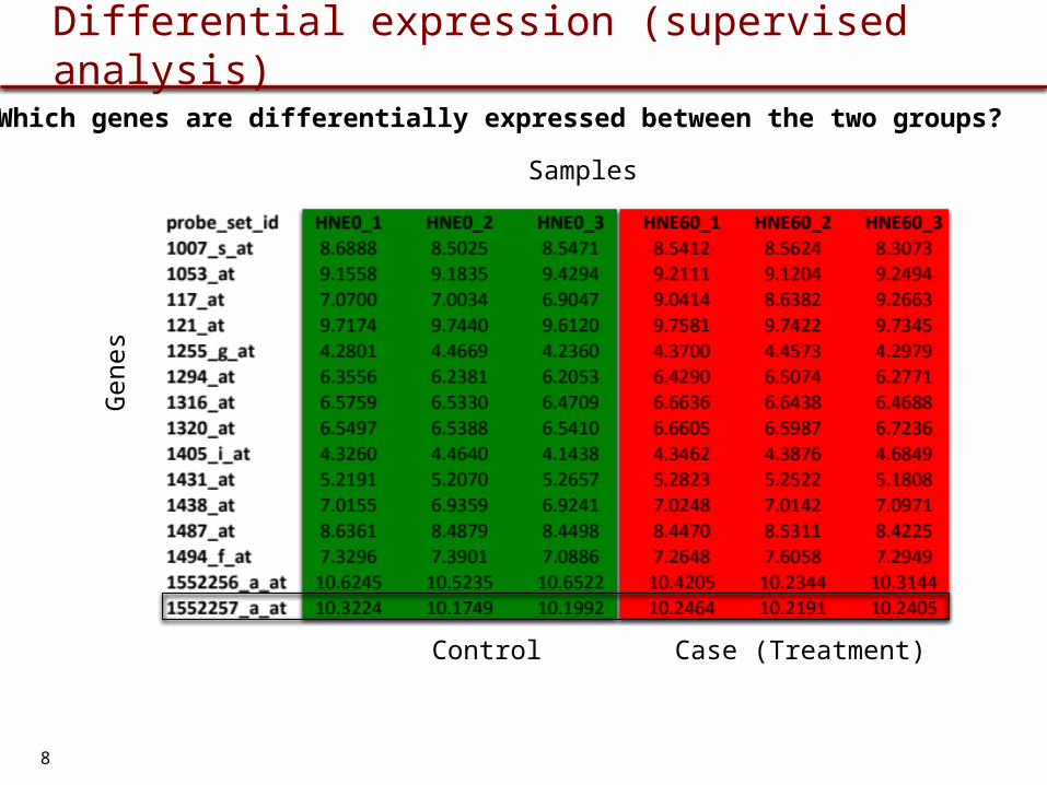
Differential expression (supervised analysis)
Control Case (Treatment)
Gen
es
Samples
Which genes are differentially expressed between the two groups?
8
Fold change
n-fold change Arbitrarily selected fold change cut-offs Usually ≥ 2 fold
Pros Intuitive Simple and rapid
Cons Outlier observations can create an apparent difference Many real biological difference can not pass the 2-fold cutoff
9
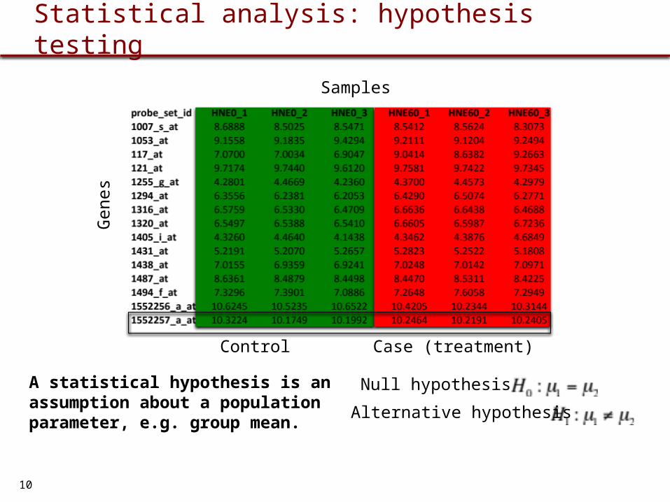
Statistical analysis: hypothesis testing
Null hypothesis
Alternative hypothesis
Control Case (treatment)
Gen
esSamples
A statistical hypothesis is an assumption about a population parameter, e.g. group mean.
10
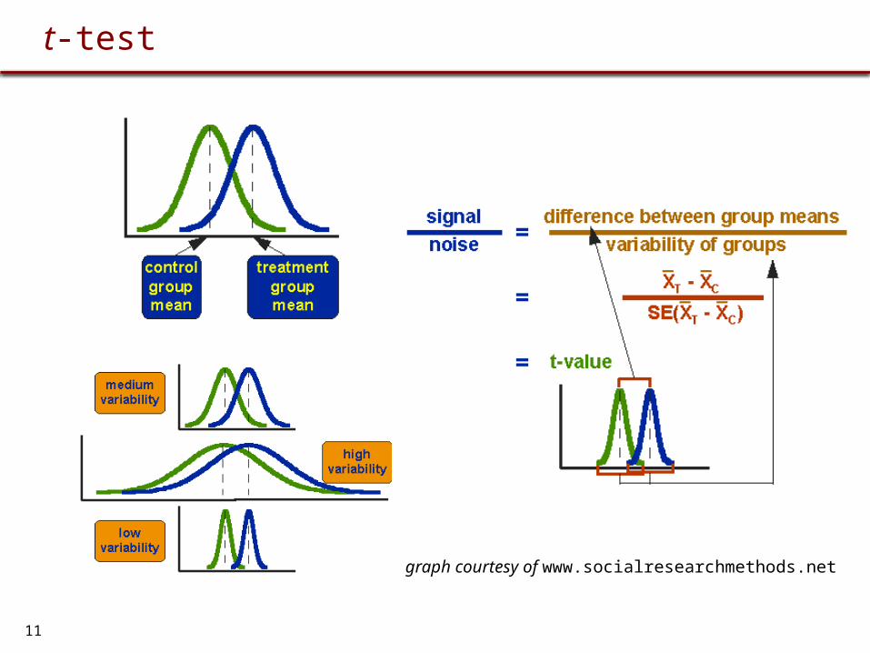
t-test
graph courtesy of www.socialresearchmethods.net
11

p value
p value: probability of more extreme test statistic, or sum of tail areas
12

Correction for multiple testing: why?
In an experiment with a 10,000-gene array in which the significance level p is set at 0.05, 10,000 x 0.05 = 500 genes would be inferred as significant even though none is differentially expressed
The probability of drawing the wrong conclusion in at least one of the n different test is
Where is the significance level at single gene level, and is the global significance level.
Eac
h ro
w is
a t
est 1 0.05 0.05
10 0.05 0.40100 0.05 0.991000 0.05 1.0010000 0.05 1.00
n
13

Correction for multiple testing: how?
Control the family-wise error rate (FWER), the probability that there is a single type I error in the entire set (family) of hypotheses tested. e.g. Standard Bonferroni Correction: uncorrected p value x no. of genes tested
Control the false discovery rate (FDR), the expected proportion of false positives among the number of rejected hypotheses. e.g. Benjamini and Hochberg correction. Ranking all genes according to their p value
Picking a desired FDR level, q (e.g. 5%)
Starting from the top of the list, accept all genes with , where i is the number of genes accepted so far, and m is the total number of genes tested.
p Bonferroni0.00003 0.00030.00004 0.00040.0003 0.0030.0008 0.0080.002 0.020.01 0.10.049 0.490.23 10.55 10.92 1
Rank (i) q (i/m)*q significant?1 0.05 0.0050 12 0.05 0.0100 13 0.05 0.0150 14 0.05 0.0200 15 0.05 0.0250 16 0.05 0.0300 17 0.05 0.0350 08 0.05 0.0400 09 0.05 0.0450 010 0.05 0.0500 0
14

Clustering (unsupervised analysis)
Clustering algorithms are methods to divide a set of n objects (genes or samples) into g groups so that within group similarities are larger than between group similarities
Unsupervised techniques that do not require sample annotation in the process
Identify candidate subgroups in complex data. e.g. identification of novel sub-types in cancer, identification of co-expressed genes
Sample_1 Sample_2 Sample_3 Sample_4 Sample_5 ……TNNC1 14.82 14.46 14.76 11.22 11.55 ……DKK4 10.71 10.37 11.23 19.74 19.73 ……ZNF185 15.20 14.96 15.07 12.57 12.37 ……CHST3 13.40 13.18 13.15 11.18 10.99 ……FABP3 15.87 15.80 15.85 13.16 12.99 ……MGST1 12.76 12.80 12.67 14.92 15.02 ……DEFA5 10.63 10.47 10.54 15.52 15.52 ……VIL1 11.47 11.69 11.87 13.94 14.01 ……AKAP12 18.26 18.10 18.50 15.60 15.69 ……HS3ST1 10.61 10.67 10.50 12.44 12.23 ………… …… …… …… …… …… ……
Gen
es
Samples
15

Hierarchical clustering
Agglomerative hierarchical clustering (bottom-up) Start out with all sample units in n
clusters of size 1.
At each step of the algorithm, the pair of clusters with the shortest distance are combined into a single cluster.
The algorithm stops when all sample units are combined into a single cluster of size n.
Require distance measurement Between two objects
Between clusters
16

Between objects distance measurement Euclidean distance
Focus on the absolute expression value Pearson correlation coefficient
Focus on the expression profile shape Linear relationship
Spearman correlation coefficient Focus on the expression profile shape Monotonic relationship Less sensitive but more robust than Pearson
17
Sample_1 Sample_2 Sample_3 Sample_4 Sample_5 ……TNNC1 14.82 14.46 14.76 11.22 11.55 ……DKK4 10.71 10.37 11.23 19.74 19.73 ……ZNF185 15.20 14.96 15.07 12.57 12.37 ……CHST3 13.40 13.18 13.15 11.18 10.99 ……FABP3 15.87 15.80 15.85 13.16 12.99 ………… …… …… …… …… …… ……

Different measurement, different distance
0
1
2
3
4
5
6
1 2 3 4 5 6 7
Time (hr)G
en
e e
xp
res
sio
n le
ve
l (lo
g2
)
GeneA
GeneB
GeneC
GeneD
Most similar profile to GeneA (blue) based on different distance measurement:Euclidean: GeneB (pink)
Pearson: GeneC (green)
Spearman: GeneD (red)
18

Between cluster distance measurement
Single linkage: the smallest distance of all pairwise distances Complete linkage: the maximum distance of all pairwise distances Average linkage: the average distance of all pairwise distances
19

Visualization of hierarchical clustering results
Dendrogram Output of a hierarchical
clustering Tree structure with the genes
or samples as the leaves The height of the join indicates
the distance between the branches
Heat map Graphical representation of
data where the values are represented as colors.
20

Example #1
21
Clustered display of data from time course of serum stimulation of primary human fibroblasts. the sequence-verified named genes in these clusters contain multiple genes involved in (A) cholesterol biosynthesis, (B) the cell cycle, (C) the immediate–early response, (D) signaling and angiogenesis, and (E) wound healing and tissue remodeling. These clusters also contain named genes not involved in these processes and numerous uncharacterized genes.
Eisen et al. Cluster analysis and display of genome-wide expression patterns. PNAS, 1998

Example #2
22
Sorlie et al. Gene expression patterns of breast carcinomas distinguish tumor subclasses with clinical implications. PNAS, 2001

Summary
Three major goals of gene expression studies
Differential expression (supervised analysis)
Clustering (unsupervised analysis)
Classification (machine learning)
Gene expression data pre-processing steps
Missing data imputation
Normalization
Transformation
Differential expression analysis
Student’s t-test
Multiple-test adjustment
Control the family-wise error rate (FWER)
Control the false discovery rate (FDR)
23
Agglomerative hierarchical clustering
Bottom-up
Between objects distance measurement Euclidean distance Pearson’s correlation coefficient Spearman’s correlation coefficient
Between cluster distance measurement
Single linkage
Complete linkage
Average linkage
Visualization
Dendrogram
Heat map

Reading
24
Sabates-Bellver et al., Mol Cancer Res, 5(12):1263-1275, 2007