Supplement of Effects of dust ... - atmos-chem-phys.net · We conclude that the dipole resolution used caused relative errors of 1-10% at large size parameters, depending on the scattering

Supplement of Atmos. Chem. Phys., 15, 12011–12028, 2015http://www.atmos-chem-phys.net/15/12011/2015/doi:10.5194/acp-15-12011-2015-supplement© Author(s) 2015. CC Attribution 3.0 License.

Supplement of

Effects of dust particle internal structure on light scattering

O. Kemppinen et al.

Correspondence to:O. Kemppinen ([email protected])

The copyright of individual parts of the supplement might differ from the CC-BY 3.0 licence.

This supplementary document provides more details on a few potentialtechnical questions the reader might have: DDA accuracy with the chosendipole resolution, the effect of particle variability within the three-particleensemble used, and the choice of effective medium approximation.

1 DDA accuracy

We have employed the -jagged option of ADDA to study the inaccuraciesrelated to shape determination. Unfortunately, even -jagged 2 consumesroughly 8 times as much CPU time, which would be almost one million CPUhours for the full runs, which would take several months with the computingresources available to us. Instead, we have decided to perform limited tests,and only for -jagged 2 (double dipole resolution along each axis, 8 timesthe total number of dipoles) instead of e.g. -jagged 4 (quadruple dipoleresolution along each axis, 64 times the total number of dipoles).

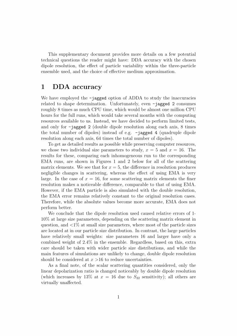
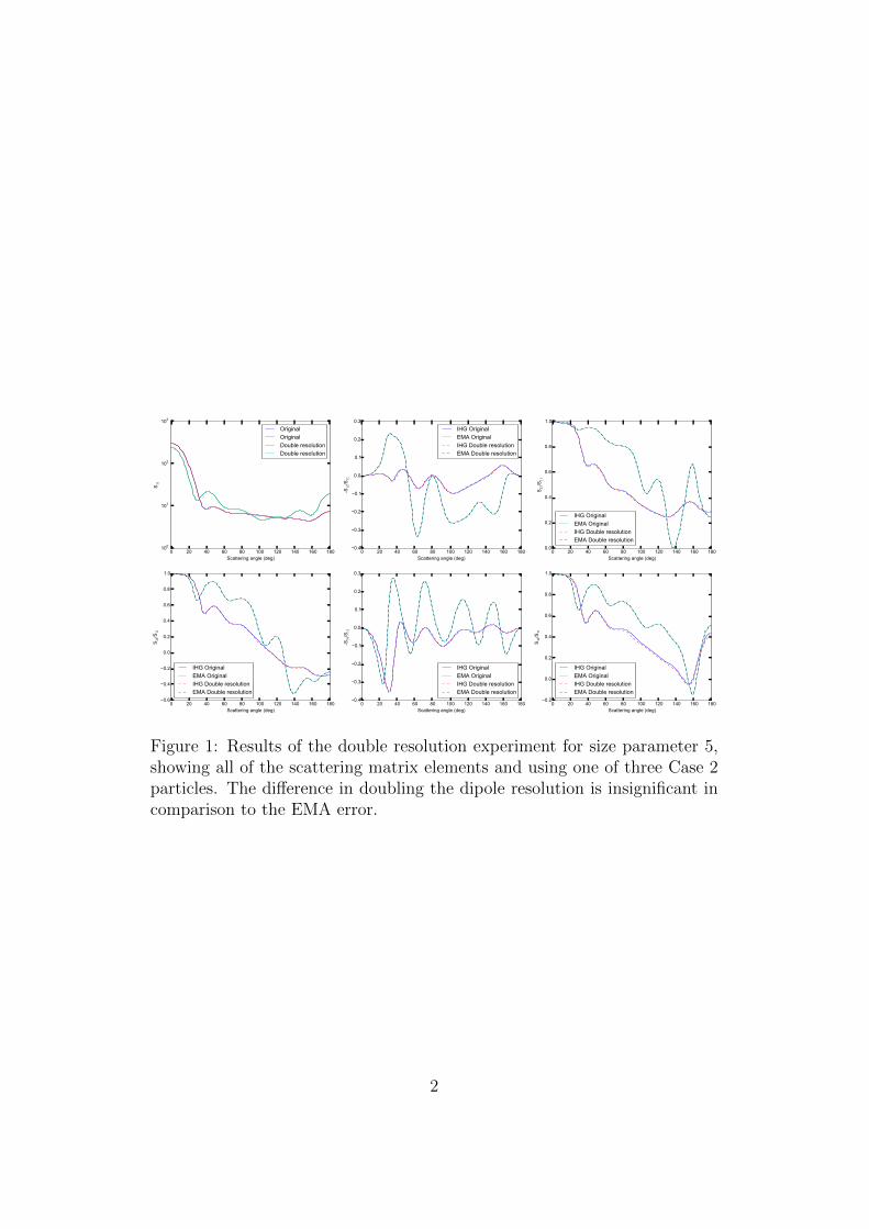
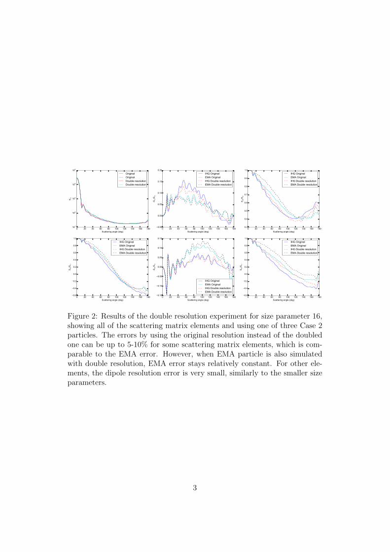
To get as detailed results as possible while preserving computer resources,we chose two individual size parameters to study, x = 5 and x = 16. Theresults for these, comparing each inhomogeneous run to the correspondingEMA runs, are shown in Figures 1 and 2 below for all of the scatteringmatrix elements. We see that for x = 5, the difference in resolution producesnegligible changes in scattering, whereas the effect of using EMA is verylarge. In the case of x = 16, for some scattering matrix elements the finerresolution makes a noticeable difference, comparable to that of using EMA.However, if the EMA particle is also simulated with the double resolution,the EMA error remains relatively constant to the original resolution cases.Therefore, while the absolute values become more accurate, EMA does notperform better.

We conclude that the dipole resolution used caused relative errors of 1-10% at large size parameters, depending on the scattering matrix element inquestion, and <1% at small size parameters, where most of the particle sizesare located at in our particle size distribution. In contrast, the large particleshave relatively small weights: size parameters 16 and larger have only acombined weight of 2.4% in the ensemble. Regardless, based on this, extracare should be taken with wider particle size distributions, and while themain features of simulations are unlikely to change, double dipole resolutionshould be considered at x >16 to reduce uncertainties.

As a final note, of the scalar scattering quantities considered, only thelinear depolarization ratio is changed noticeably by double dipole resolution(which increases by 13% at x = 16 due to S22 sensitivity); all others arevirtually unaffected.

1

0 20 40 60 80 100 120 140 160 180Scattering angle (deg)

100

101

102

103

S 11

OriginalOriginalDouble resolutionDouble resolution


0.4

0.3

0.2

0.1

0.0

0.1

0.2

0.3

-S12

/S11

IHG OriginalEMA OriginalIHG Double resolutionEMA Double resolution


0.0

0.2

0.4

0.6

0.8

1.0

S 22/S

11



0.6

0.4

0.2

0.0

0.2

0.4

0.6

0.8

1.0

S 33/S

11



0.4

0.3

0.2

0.1

0.0

0.1

0.2

0.3

-S34

/S11



0.2

0.0

0.2

0.4

0.6

0.8

1.0

S 44/S

11


Figure 1: Results of the double resolution experiment for size parameter 5,showing all of the scattering matrix elements and using one of three Case 2particles. The difference in doubling the dipole resolution is insignificant incomparison to the EMA error.

2


101

102

103

104

105

S 11

OriginalOriginalDouble resolutionDouble resolution


0.05

0.00

0.05

0.10

0.15

0.20

-S12/S

11



0.3

0.4

0.5

0.6

0.7

0.8

0.9

1.0

S 22/S

11



0.6

0.4

0.2

0.0

0.2

0.4

0.6

0.8

1.0

S 33/S

11



0.15

0.10

0.05

0.00

0.05

0.10

0.15

-S34

/S11



0.6

0.4

0.2

0.0

0.2

0.4

0.6

0.8

1.0S 4

4/S11


Figure 2: Results of the double resolution experiment for size parameter 16,showing all of the scattering matrix elements and using one of three Case 2particles. The errors by using the original resolution instead of the doubledone can be up to 5-10% for some scattering matrix elements, which is com-parable to the EMA error. However, when EMA particle is also simulatedwith double resolution, EMA error stays relatively constant. For other ele-ments, the dipole resolution error is very small, similarly to the smaller sizeparameters.

3

2 Shape ensembles

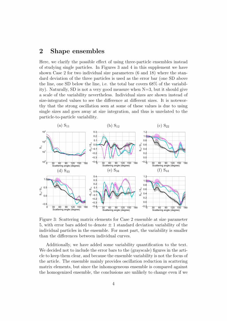
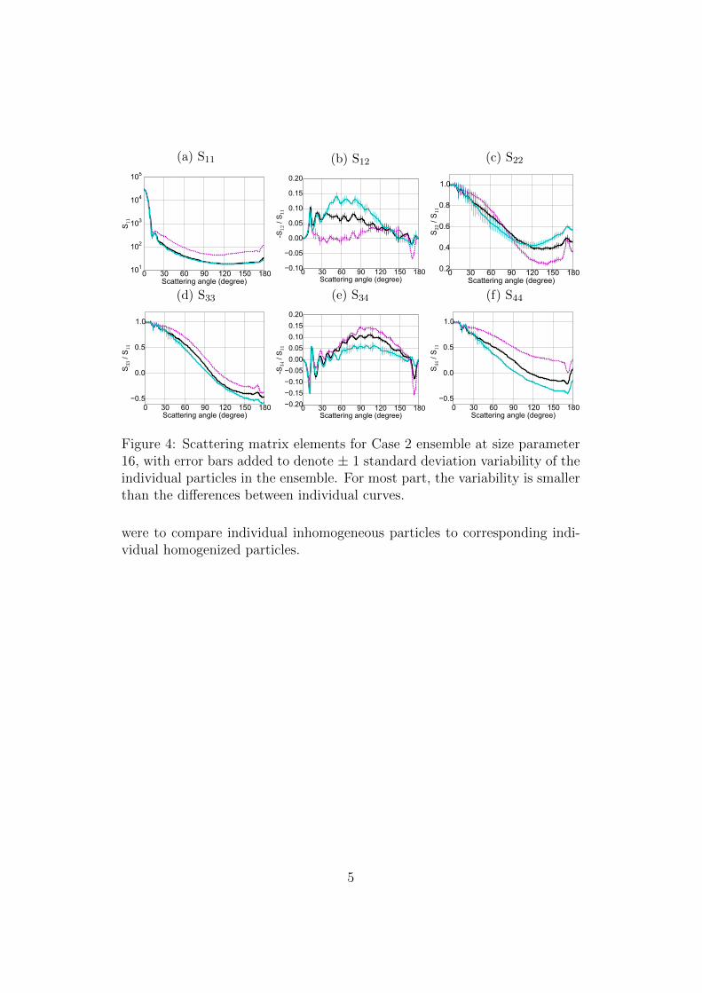
Here, we clarify the possible effect of using three-particle ensembles insteadof studying single particles. In Figures 3 and 4 in this supplement we haveshown Case 2 for two individual size parameters (6 and 18) where the stan-dard deviation of the three particles is used as the error bar (one SD abovethe line, one SD below the line, i.e. the total bar covers 68% of the variabil-ity). Naturally, SD is not a very good measure when N=3, but it should givea scale of the variability nevertheless. Individual sizes are shown instead ofsize-integrated values to see the difference at different sizes. It is notewor-thy that the strong oscillation seen at some of these values is due to usingsingle sizes and goes away at size integration, and thus is unrelated to theparticle-to-particle variability.

(a) S11

0 30 60 90 120 150 180Scattering angle (degree)

100

101

102

103

S 11

(b) S12


0.4

0.3

0.2

0.1

0.0

0.1

0.2

0.3

-S12

/ S 1

1

(c) S22


0.2

0.0

0.2

0.4

0.6

0.8

1.0

1.2

S 22 /

S 11

(d) S33


0.5

0.0

0.5

1.0

S 33 /

S11

(e) S34


0.40.30.20.10.00.10.20.30.4

-S34

/ S 1

1

(f) S44


0.2

0.0

0.2

0.4

0.6

0.8

1.0

1.2

S 44 /

S 11

Figure 3: Scattering matrix elements for Case 2 ensemble at size parameter5, with error bars added to denote ± 1 standard deviation variability of theindividual particles in the ensemble. For most part, the variability is smallerthan the differences between individual curves.

Additionally, we have added some variability quantification to the text.We decided not to include the error bars to the (grayscale) figures in the arti-cle to keep them clear, and because the ensemble variability is not the focus ofthe article. The ensemble mainly provides oscillation reduction in scatteringmatrix elements, but since the inhomogeneous ensemble is compared againstthe homogenized ensemble, the conclusions are unlikely to change even if we

4

(a) S11


101

102

103

104

105

S 11

(b) S12


0.10

0.05

0.00

0.05

0.10

0.15

0.20

-S12

/ S 1

1

(c) S22


0.2

0.4

0.6

0.8

1.0

S 22 /

S11

(d) S33


0.5

0.0

0.5

1.0

S 33 /

S 11

(e) S34


0.200.150.100.050.000.050.100.150.20

-S34

/ S 1

1

(f) S44


0.5

0.0

0.5

1.0

S 44 /

S11

Figure 4: Scattering matrix elements for Case 2 ensemble at size parameter16, with error bars added to denote ± 1 standard deviation variability of theindividual particles in the ensemble. For most part, the variability is smallerthan the differences between individual curves.

were to compare individual inhomogeneous particles to corresponding indi-vidual homogenized particles.

5

3 Effective medium approximation selection

When testing the performance of EMA’s, an especially when making a claimthat EMA’s (in general) can not replicate scattering, it is important to testdifferent EMA methods and select the most appropriate one. Here, we testfive different EMA’s: normal and inverse Maxwell Garnett (MG), Brugge-man, volume average of refractive indices, and volume average of permittivi-ties. Due to heavy computational costs we did not perform the full scatteringcalculations for all of these. Instead, we chose two cases, Case 2 and Case5, to test, due to the fact that their hematite content likely has the greatesteffect on EMA’s. Additionally, instead of studying the size distribution inte-grated values, we study two individual sizes, x = 5 andx = 16, to see if andhow the EMA validity changes as a function of the size parameter.

Case 2 is simplified by considering only 2 materials instead of the original12, because the traditional MG is applicable to only 2 materials. We havethus chosen as the materials to study a bulk clay mineral with refractive indexof 1.55 + i0 and volume fraction of 85%, and hematite with refractive indexof 3.09 + i0.0925 and volume fraction of 15%. The EMA of this simplifiedsystem obtained by volume average of refractive indices is 1.78 + i0.0139,close to the original Case 2 EMA m of 1.78 + i0.0135. Because the clayminerals in the original inhomogeneous particles have very similar refractiveindices (most of the minerals are within between refractive indices 1.52 and1.57, with roughly 6% of the total volume having refractive indices of up to1.60), and based on the close match in the homogenized refractive indicesbetween the original and the simplified versions, we conclude that it is likelythat this simplified case is representative of the original case.

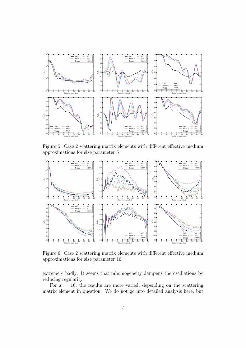
We have chosen to replicate the results with five different EMA’s usingthis simplified composition: the original way of averaging refractive indices(1.78 + i0.0139), averaging permittivities (1.86 + i0.0230), MG using largervolume fraction as the matrix (MG1, 1.73 + i0.0073), MG using larger vol-ume fraction as the inclusion (MG2, 1.80 + i0.0172), and Bruggeman (1.74+ i0.0089). It is very important to note that the particles in this study aregenerally not within the validity criteria of the EMA’s, which also may helpto explain the results below. For example, the assumption that the inclu-sions are much smaller than the wavelength does not hold for the particlesconsidered here. It could be argued that highly localized and spatially non-uniformly distributed inhomogeneity is very hard to represent by any simpleparametrization, unless specifically tuned for each individual particle andeven size parameter. These results are visualized in Figures 5 and 6 belowfor size parameters 5 and 16, respectively.

The results show that for x = 5, on average, all EMA’s tested perform

6


100

101

102

103

S 11

IHGMean mBrugg.

MG1MG2Mean ε


0.4

0.3

0.2

0.1

0.0

0.1

0.2

0.3

0.4

-S12/S

11

IHGMean mBrugg.

MG1MG2Mean ε


0.2

0.0

0.2

0.4

0.6

0.8

1.0

S 22/S

11

IHGMean mBrugg.

MG1MG2Mean ε


0.6

0.4

0.2

0.0

0.2

0.4

0.6

0.8

1.0

S 33/S

11

IHGMean mBrugg.

MG1MG2Mean ε


0.4

0.3

0.2

0.1

0.0

0.1

0.2

0.3-S

34/S

11

IHGMean mBrugg.

MG1MG2Mean ε


0.4

0.2

0.0

0.2

0.4

0.6

0.8

1.0

S 44/S

11

IHGMean mBrugg.

MG1MG2Mean ε

Figure 5: Case 2 scattering matrix elements with different effective mediumapproximations for size parameter 5


101

102

103

104

105

S 11

IHGMean mBrugg.

MG1MG2Mean ε


0.05

0.00

0.05

0.10

0.15

0.20

0.25

-S12

/S11

IHGMean mBrugg.

MG1MG2Mean ε


0.3

0.4

0.5

0.6

0.7

0.8

0.9

1.0

S 22/S

11

IHGMean mBrugg.

MG1MG2Mean ε


0.8

0.6

0.4

0.2

0.0

0.2

0.4

0.6

0.8

1.0

S 33/S

11

IHGMean mBrugg.

MG1MG2Mean ε


0.20

0.15

0.10

0.05

0.00

0.05

0.10

0.15

-S34

/S11

IHGMean mBrugg.

MG1MG2Mean ε


0.6

0.4

0.2

0.0

0.2

0.4

0.6

0.8

1.0

S 44/S

11

IHGMean mBrugg.

MG1MG2Mean ε


extremely badly. It seems that inhomogeneity dampens the oscillations byreducing regularity.

For x = 16, the results are more varied, depending on the scatteringmatrix element in question. We do not go into detailed analysis here, but

7

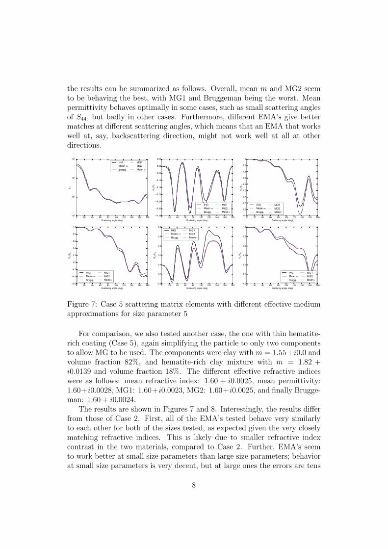
the results can be summarized as follows. Overall, mean m and MG2 seemto be behaving the best, with MG1 and Bruggeman being the worst. Meanpermittivity behaves optimally in some cases, such as small scattering anglesof S44, but badly in other cases. Furthermore, different EMA’s give bettermatches at different scattering angles, which means that an EMA that workswell at, say, backscattering direction, might not work well at all at otherdirections.


100

101

102

103

S 11

IHGMean mBrugg.

MG1MG2Mean ε


0.35

0.30

0.25

0.20

0.15

0.10

0.05

0.00

0.05

-S12/S

11

IHGMean mBrugg.

MG1MG2Mean ε


0.1

0.2

0.3

0.4

0.5

0.6

0.7

0.8

0.9

1.0

S 22/S

11

IHGMean mBrugg.

MG1MG2Mean ε


0.6

0.4

0.2

0.0

0.2

0.4

0.6

0.8

1.0

S 33/S

11

IHGMean mBrugg.

MG1MG2Mean ε


0.2

0.1

0.0

0.1

0.2

0.3

0.4

-S34

/S11

IHGMean mBrugg.

MG1MG2Mean ε


0.2

0.0

0.2

0.4

0.6

0.8

1.0

S 44/S

11

IHGMean mBrugg.

MG1MG2Mean ε


For comparison, we also tested another case, the one with thin hematite-rich coating (Case 5), again simplifying the particle to only two componentsto allow MG to be used. The components were clay with m = 1.55+ i0.0 andvolume fraction 82%, and hematite-rich clay mixture with m = 1.82 +i0.0139 and volume fraction 18%. The different effective refractive indiceswere as follows: mean refractive index: 1.60 + i0.0025, mean permittivity:1.60+i0.0028, MG1: 1.60+i0.0023, MG2: 1.60+i0.0025, and finally Brugge-man: 1.60 + i0.0024.

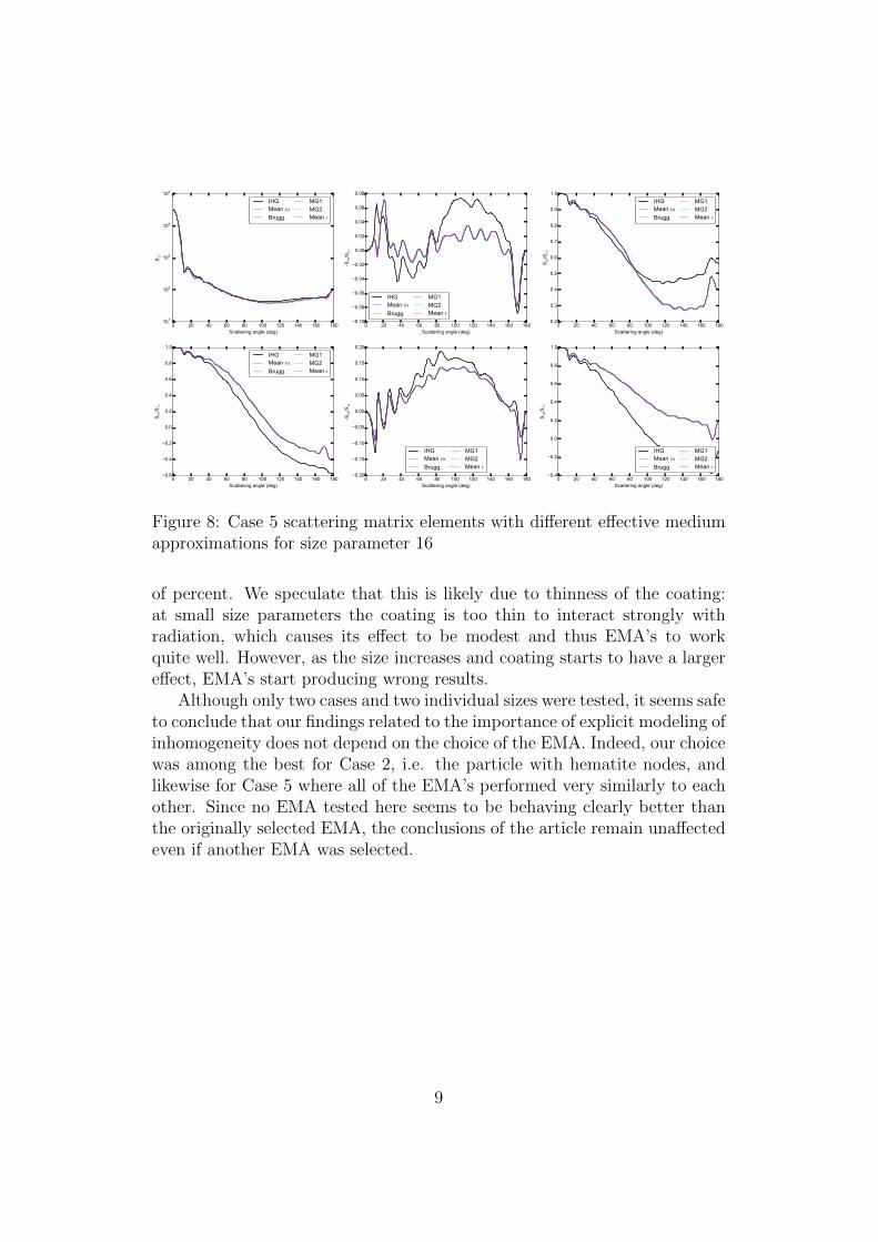
The results are shown in Figures 7 and 8. Interestingly, the results differfrom those of Case 2. First, all of the EMA’s tested behave very similarlyto each other for both of the sizes tested, as expected given the very closelymatching refractive indices. This is likely due to smaller refractive indexcontrast in the two materials, compared to Case 2. Further, EMA’s seemto work better at small size parameters than large size parameters; behaviorat small size parameters is very decent, but at large ones the errors are tens

8


101

102

103

104

105

S 11

IHGMean mBrugg.

MG1MG2Mean ε


0.10

0.08

0.06

0.04

0.02

0.00

0.02

0.04

0.06

0.08

-S12/S

11

IHGMean mBrugg.

MG1MG2Mean ε


0.2

0.3

0.4

0.5

0.6

0.7

0.8

0.9

1.0

S 22/S

11

IHGMean mBrugg.

MG1MG2Mean ε


0.6

0.4

0.2

0.0

0.2

0.4

0.6

0.8

1.0

S 33/S

11

IHGMean mBrugg.

MG1MG2Mean ε


0.20

0.15

0.10

0.05

0.00

0.05

0.10

0.15

0.20-S

34/S

11

IHGMean mBrugg.

MG1MG2Mean ε


0.4

0.2

0.0

0.2

0.4

0.6

0.8

1.0

S 44/S

11

IHGMean mBrugg.

MG1MG2Mean ε


of percent. We speculate that this is likely due to thinness of the coating:at small size parameters the coating is too thin to interact strongly withradiation, which causes its effect to be modest and thus EMA’s to workquite well. However, as the size increases and coating starts to have a largereffect, EMA’s start producing wrong results.

Although only two cases and two individual sizes were tested, it seems safeto conclude that our findings related to the importance of explicit modeling ofinhomogeneity does not depend on the choice of the EMA. Indeed, our choicewas among the best for Case 2, i.e. the particle with hematite nodes, andlikewise for Case 5 where all of the EMA’s performed very similarly to eachother. Since no EMA tested here seems to be behaving clearly better thanthe originally selected EMA, the conclusions of the article remain unaffectedeven if another EMA was selected.

9

Documents

Supplement of Effects of dust ... - atmos-chem-phys.net · We conclude that the dipole resolution used caused relative errors of 1-10% at large size parameters, depending on the scattering