Embed Size (px)
Citation preview

Supplement of Nat. Hazards Earth Syst. Sci., 17, 2199–2211, 2017https://doi.org/10.5194/nhess-17-2199-2017-supplement© Author(s) 2017. This work is distributed underthe Creative Commons Attribution 3.0 License.
Supplement of
Climate change impacts on flood risk and asset damages within mapped100-year floodplains of the contiguous United StatesCameron Wobus et al.
Correspondence to: Cameron Wobus ([email protected])
The copyright of individual parts of the supplement might differ from the CC BY 3.0 License.
1
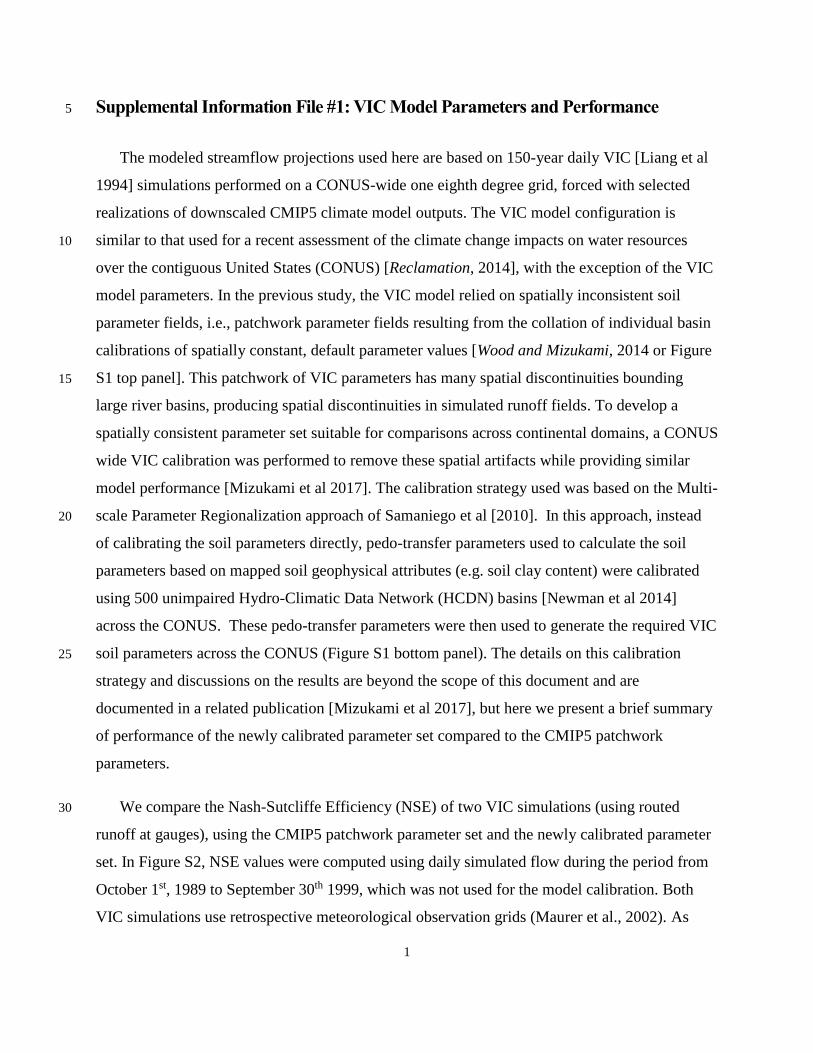
Supplemental Information File #1: VIC Model Parameters and Performance 5
The modeled streamflow projections used here are based on 150-year daily VIC [Liang et al
1994] simulations performed on a CONUS-wide one eighth degree grid, forced with selected
realizations of downscaled CMIP5 climate model outputs. The VIC model configuration is
similar to that used for a recent assessment of the climate change impacts on water resources 10
over the contiguous United States (CONUS) [Reclamation, 2014], with the exception of the VIC
model parameters. In the previous study, the VIC model relied on spatially inconsistent soil
parameter fields, i.e., patchwork parameter fields resulting from the collation of individual basin
calibrations of spatially constant, default parameter values [Wood and Mizukami, 2014 or Figure
S1 top panel]. This patchwork of VIC parameters has many spatial discontinuities bounding 15
large river basins, producing spatial discontinuities in simulated runoff fields. To develop a
spatially consistent parameter set suitable for comparisons across continental domains, a CONUS
wide VIC calibration was performed to remove these spatial artifacts while providing similar
model performance [Mizukami et al 2017]. The calibration strategy used was based on the Multi-
scale Parameter Regionalization approach of Samaniego et al [2010]. In this approach, instead 20
of calibrating the soil parameters directly, pedo-transfer parameters used to calculate the soil
parameters based on mapped soil geophysical attributes (e.g. soil clay content) were calibrated
using 500 unimpaired Hydro-Climatic Data Network (HCDN) basins [Newman et al 2014]
across the CONUS. These pedo-transfer parameters were then used to generate the required VIC
soil parameters across the CONUS (Figure S1 bottom panel). The details on this calibration 25
strategy and discussions on the results are beyond the scope of this document and are
documented in a related publication [Mizukami et al 2017], but here we present a brief summary
of performance of the newly calibrated parameter set compared to the CMIP5 patchwork
parameters.
We compare the Nash-Sutcliffe Efficiency (NSE) of two VIC simulations (using routed 30
runoff at gauges), using the CMIP5 patchwork parameter set and the newly calibrated parameter
set. In Figure S2, NSE values were computed using daily simulated flow during the period from
October 1st, 1989 to September 30th 1999, which was not used for the model calibration. Both
VIC simulations use retrospective meteorological observation grids (Maurer et al., 2002). As

2
shown in Figure S2, model performance is similar in terms of the spatial pattern and the 35
magnitude of the NSE values because some of these basins are inherently hard to model due to
errors in the forcing dataset (e.g. in the desert Southwest) and due to features of the landscape
that are not represented in the VIC model (e.g. tile drains in the Northern mid-West). Overall,
NSE values are very slightly reduced in the new dataset because the calibration was more
constrained, i.e. the VIC model parameters were not directly calibrated; however, the new 40
calibration is likely to perform equally well in ungauged basins, while the default parameter set
is likely to perform better in basins it was directly calibrated for. Importantly, the artifacts in the
spatial parameter distribution are removed in the newly calibrated parameters (Figure S1).
45

3
Supplemental Information File #2: Uncertainty Analysis for Baseline 1% AEP
Estimates
We used a bootstrapping method to estimate the uncertainty on the baseline 1% AEP event,
based on a random sample of 1,000 nodes in the modeling domain. Our approach was as follows:
1) At each randomly selected node, we first extracted the complete set of 580 annual 50
maximum flow values from the baseline period (20 years x 29 models = 580 annual
values). We calculated the 1% AEP event from this full set of annual maxima by fitting a
GEV distribution to the events, using the maximum likelihood method for finding the
GEV parameters. We then extracted the 1% AEP event by extracting the 99th percentile
value from the GEV fit. This was the 1% AEP value utilized in the remainder of the 55
analyses described in the manuscript.
2) From these 580 annual maximum values, we then selected 500 random samples of
300 values each. For each of these 500 random samples, we repeated the process of
fitting the GEV and extracting the 99th percentile value. The result of this exercise is a
set of 500 estimates of the 1% AEP event for that node (see Figure S3). 60
3) From this distribution of 500 estimates for the 1% AEP event at each node, we calculated
the 5th and 95th percentile values, and saved these values along with the value calculated
from the full suite of 580 annual maxima.
4) We used the 5th and 95th percentile values to estimate the uncertainty in the 1% AEP
event, as a percent of the estimate from the full set of 580 values. The result is a 65
distribution of uncertainties in the 1% AEP event, expressed as a percent (Figure S4).
5) Using the modal value of uncertainty on the 1% AEP event of approximately 10%
(Figure S4), we propagated this uncertainty through our estimate of the number of floods
occurring in each year of our simulation, as follows
a. We generated a normal distribution of error values ranging from approximately 70
-20% to +20%

4
b. At each node, we randomly selected a value from this distribution and multiplied
the estimated 1% AEP flood value by this random number
c. We then calculated the timeseries of flooding at each node based on this
“perturbed” 1% AEP event, and assembled a new version of Figure 5 based on 75
this perturbed timeseries (Figure S5)
Based on this qualitative comparison, as shown in Figure S5, the intermodel variability in the
timeseries of flooding overwhelms the uncertainty introduced by propagating the error in the 1%
AEP event through all of the calculations.
80

5
Supplemental Information File #3: Estimating flood depth and Asset Damages from
1% annual exceedance probability events
For each of the mapped floodplains in CONUS, we estimated flood damages using an 85
experimental tool developed for the U.S. Army Corps of Engineers, referred to as the National
Flood Risk Characterization Tool (NFRCT)1. The NFRCT includes asset exposure and damage
estimates for the 1% (“100-year”) and 0.2 % (“500-year”) annual exceedance probability flood
events, as determined by FEMA and compiled in the National Flood Hazard Layer (NFHL) 2.
Because the 100-year floodplain maps are substantially more comprehensive than the 500-year 90
floodplain maps across the United States, we focused our analysis of damages on the assets
within the 1% annual chance floodplains.
All of the steps we took to calculate asset damages were conducted in a spatially explicit
framework, utilizing publicly available data on topography, floodplain extent, and assets. 95
Damages from a 1% AEP flood were calculated for each of the mapped 1% annual probability
floodplains in the NFHL as follows:
1. Intersect NFHL polygons and Census blocks3 to create a new set of flood zone polygons
subdivided by census block boundaries. 100
2. Query the National Elevation Dataset (NED) 4 along the perimeter of each flood polygon
to determine the elevation of the 1% annual probability flood level along that perimeter.
1 Developed by Abt Associates, Inc. for the Institute for Water Resources of the U.S. Army Corps of Engineers. More information can be found at:
http://www.iwr.usace.army.mil/Portals/70/docs/frmp/Flood_Risk_Char/NFRCT_Slides_FRM_wkshp_v1.pdf. 2 FEMA (2015). National Flood Hazard Layer (NFHL). Federal Emergency Management Agency. Washington,
D.C. Available at: https://www.fema.gov/national-flood-hazard-layer-nfhl 3 Census Bureau (2010). 2010 Topologically Integrated Geographic Encoding and Referencing (TIGER)/Line
Shapefiles. Released beginning November 30, 2010. Last update March 26, 2012. U.S. Census Bureau. Suitland,
MD. ftp://ftp2.census.gov/geo/tiger/TIGER2010/ 4 USGS: National Elevation Dataset (NED), U.S. Department of the Interior, U.S. Geological Survey, Available:
https://lta.cr.usgs.gov/NED, 2016.

6
3. Randomly sample points within the interior of each of flood zone polygon to estimate the
distribution of flood water depths within each polygon (sample consists of hundreds to
thousands of points, depending on the size of the intersection area in (1)). 105
a. First, at each randomly selected point, query the NED to find the ground level
elevation at that location.
b. Second, calculate the elevation of the flood surface using a nearest neighbor
sampling method. The interior flood water elevation is calculated as a weighted
average of sampled perimeter points around each randomly selected point. 110
c. Compute the difference between the elevation of the estimated water surface and
the ground level elevation. This value approximates the depth of a 1% annual
exceedance probability flood event at this point.
4. For the sampled interior points, use the National Land Cover Dataset5 to determine
whether each point is categorized as “Developed” or not; track depth estimates separately 115
for developed and undeveloped points within each polygon.
5. From the randomly sampled points within the interior of each flood zone polygon,
calculate odd depth percentiles (1st, 3rd, 5th,…,99th) for each flood zone.
The result of this process is a distribution (described by percentiles) of flood depths for each 120
NFHL-Census Block intersection. For each intersection, three distributions are generated: 1)
depths throughout the polygon, 2) depths within areas designated as Developed, and 3) depths
within areas designated as Undeveloped. From these results, the following steps are used to
calculate monetary damages:
125
5 Homer, C.G., Dewitz, J.A., Yang, L., Jin, S., Danielson, P., Xian, G., Coulston, J., Herold, N.D.,
Wickham, J.D., and Megown, K., 2015, Completion of the 2011 National Land Cover Database for the
conterminous United States-Representing a decade of land cover change information. Photogrammetric Engineering and Remote Sensing, v. 81, no. 5, p. 345-354

7
1. For the “Developed” portions of the NFHL-Census block intersection, data on built assets
are tabulated from FEMA’s HAZUS-MH6 General Building Stock inventory. The
General Building Stock inventory provides estimates of the number and aggregate dollar
value of multiple types of residential, commercial, and industrial buildings for each
Census block. 130
2. The number and value of buildings and contents that are exposed to flood inundation is
equal to the percentage of the Developed portion of a Census block that is intersected by
a NFHL flood zone multiplied by the corresponding total number of residential assets and
their values within the block. Buildings and aggregate building value are assumed to be
evenly distributed across the Developed portions of each Census Block. For example, if 135
50% of the developed portion of a block is intersected by a floodzone, it is assumed that
50% of that Block’s buildings and aggregate building value are exposed to flooding.
3. The same assumption is applied to estimate exposure to different depths – if the 10th
percentile of depth for given polygon is 2.5 feet, it is assumed that 10% of the developed
portion of that block, as well as 10% of its buildings and building value, is exposed to 2.5 140
feet of inundation.
4. Damage estimates are created using depth-damage functions from USACE and FEMA7.
A separate depth-damage function is used for each of 28 different categories of buildings
(e.g., residential one-story homes without a basement). Each depth damage function
describes the percent loss as a function of depth. 145
5. The depth damage functions are applied to the aggregate value for each category of
building within each NFHL-Census block intersection, using depth exposure results
described above. In other words, if it was estimated that 10% of buildings are exposed to
6 FEMA (2015). HAZUS-MH 2.2, FEMA's Software Program for Multi-Hazard Loss Estimation for Potential
Losses from Disaster. Federal Emergency Management Agency. Washington, D.C. 7 USACE (2000). Economic Guidance Memorandum (EGM 01-03): Generic Depth-Damage Relationships.
http://planning.usace.army.mil/toolbox/library/EGMs/egm01-03.pdf
USACE (2003). Economic Guidance Memorandum (EGM) 04-01, Generic Depth-Damage Relationships for
Residential Structures with Basements. http://planning.usace.army.mil/toolbox/library/EGMs/egm04-01.pdf
FEMA (2009a). HAZUS-MH, FEMA's Software Program for Estimating Potential Losses from Disaster. Federal
Emergency Management Agency. Washington, D.C.

8
2.5 feet of inundation, then the depth-damage estimate for 2.5 feet of inundation is
applied to 10% of the aggregate building value. 150
9
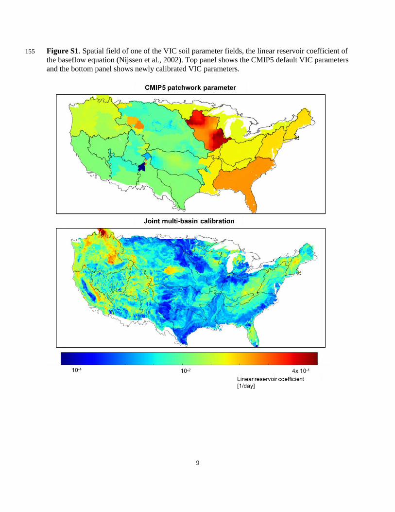
Figure S1. Spatial field of one of the VIC soil parameter fields, the linear reservoir coefficient of 155
the baseflow equation (Nijssen et al., 2002). Top panel shows the CMIP5 default VIC parameters
and the bottom panel shows newly calibrated VIC parameters.

10
Figure S2. NSE values of retrospective VIC simulations at each HCDN basin. Top panel shows 160
the results of VIC simulations using the CMIP5 VIC parameters and bottom panel shows the
results with the newly calibrated VIC parameters.
165

11
Figure S3. Example of uncertainty analysis on 1% AEP event for a single node, based on
bootstrapping method described above.

12
Figure S4. Distribution of uncertainty on 1% AEP event based on 1,000 randomly selected
nodes in the model domain. 170
13
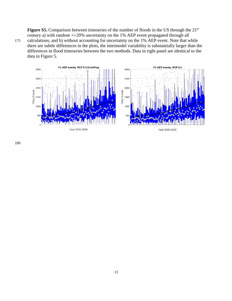
Figure S5. Comparison between timeseries of the number of floods in the US through the 21st
century a) with random +/-20% uncertainty on the 1% AEP event propagated through all
calculations, and b) without accounting for uncertainty on the 1% AEP event. Note that while 175
there are subtle differences in the plots, the intermodel variability is substantially larger than the
differences in flood timeseries between the two methods. Data in right panel are identical to the
data in Figure 5.
180

14
Supplemental Information File References
Newman, A., K. Sampson, M.P. Clark, A. Bock, and R.J. Viger, and D. Blodgett (2014), A 185
large-sample watershed-scale hydrometeorological dataset for the contiguous USA.
Boulder, CO: UCAR/NCAR. doi:10.5065/D6MW2F4D
Mizukami, N., M. P. Clark, A. J. Newman, A. W. Wood, E. D. Gutmann, B. Nijssen, L.
Samaniego, and O. Rakovec (2017), Towards seamless large domain parameter estimation
for hydrologic models, Water Resources Research. Accepted pending minor revisions 190
Reclamation: Downscaled CMIP3 and CMIP5 Climate and Hydrology Projections: Release of
Hydrology Projections, Comparison with Preceding Information, and Summary of User
Needs, Prepared by the U.S. Department of the Interior, Bureau of Reclamation, Technical
Services Center, Denver, CO, 2014.
Samaniego, L., R. Kumar, and S. Attinger (2010), Multiscale parameter regionalization of a grid-195
based hydrologic model at the mesoscale, Water Resources Research, 46(5),
doi:10.1029/2008WR007327.
Wood, A., and N. Mizukami: Project Summary Report: CMIP5 1/8 Degree Daily Weather and
VIC Hydrology Datasets for CONUS. 2014
200