Embed Size (px)
Citation preview

10
Supplement OutlineIntroduction and Sampling Plans, 2
Operating Characteristic Curve, 3
Determining Single Sampling Plans, 9
Average Quality of Inspected Lots and a Related Sampling Plan, 12
Key Terms, 14
Solved Problems, 14
Discussion and Review Questions, 16
Internet Exercises, 16
Problems, 16
Mini-case: CRYSTAL S.A., 19
Mini-case: Gustave Roussy Institute, 20
Acceptance Sampling
SUPPLEMENT TO
CHAPTER
Learning Objectives
After completing this supplement, you should be able to:
LO 1 Explain acceptance sampling, and contrast single and multiple sampling plans.
LO 2 Construct and use an operating characteristic curve.
LO 3 Determine single sampling plans.
LO 4 Determine the average quality of inspected lots, and determine a related sampling plan.
PART FOUR Quality2
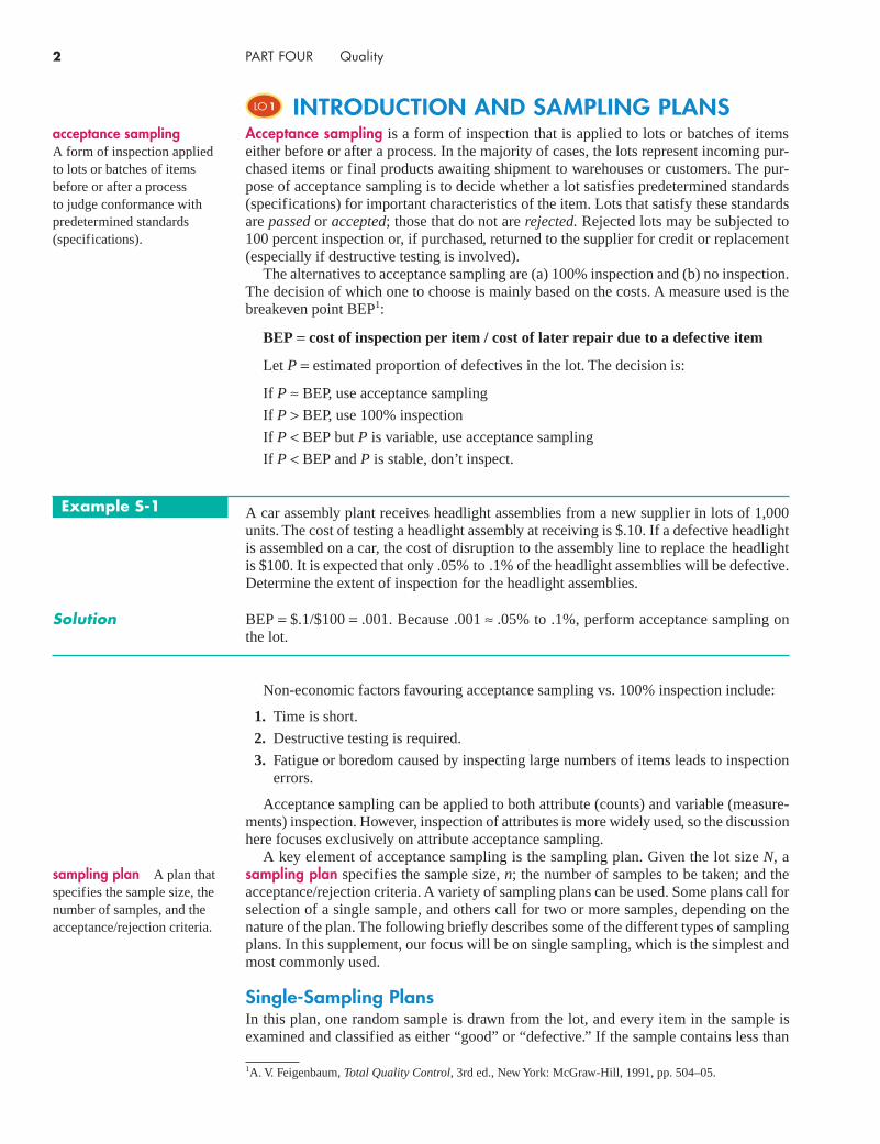
LO 1 IntroductIon And SAmplIng plAnSAcceptance sampling is a form of inspection that is applied to lots or batches of items either before or after a process. In the majority of cases, the lots represent incoming pur-chased items or final products awaiting shipment to warehouses or customers. The pur-pose of acceptance sampling is to decide whether a lot satisfies predetermined standards (specifications) for important characteristics of the item. Lots that satisfy these standards are passed or accepted; those that do not are rejected. Rejected lots may be subjected to 100 percent inspection or, if purchased, returned to the supplier for credit or replacement (especially if destructive testing is involved).
The alternatives to acceptance sampling are (a) 100% inspection and (b) no inspection. The decision of which one to choose is mainly based on the costs. A measure used is the breakeven point BEP1:
BEP = cost of inspection per item / cost of later repair due to a defective item
Let P = estimated proportion of defectives in the lot. The decision is:
If P ≈ BEP, use acceptance sampling
If P > BEP, use 100% inspection
If P < BEP but P is variable, use acceptance sampling
If P < BEP and P is stable, don’t inspect.
acceptance sampling A form of inspection applied to lots or batches of items before or after a process to judge conformance with predetermined standards (specifications).
A car assembly plant receives headlight assemblies from a new supplier in lots of 1,000 units. The cost of testing a headlight assembly at receiving is $.10. If a defective headlight is assembled on a car, the cost of disruption to the assembly line to replace the headlight is $100. It is expected that only .05% to .1% of the headlight assemblies will be defective. Determine the extent of inspection for the headlight assemblies.
example s-1
Solution BEP = $.1/$100 = .001. Because .001 ≈ .05% to .1%, perform acceptance sampling on the lot.
Non-economic factors favouring acceptance sampling vs. 100% inspection include:
Time is short.1.
Destructive testing is required.2.
Fatigue or boredom caused by inspecting large numbers of items leads to inspection 3. errors.
Acceptance sampling can be applied to both attribute (counts) and variable (measure-ments) inspection. However, inspection of attributes is more widely used, so the discussion here focuses exclusively on attribute acceptance sampling.
A key element of acceptance sampling is the sampling plan. Given the lot size N, a sampling plan specifies the sample size, n; the number of samples to be taken; and the acceptance/rejection criteria. A variety of sampling plans can be used. Some plans call for selection of a single sample, and others call for two or more samples, depending on the nature of the plan. The following briefly describes some of the different types of sampling plans. In this supplement, our focus will be on single sampling, which is the simplest and most commonly used.
Single-Sampling plansIn this plan, one random sample is drawn from the lot, and every item in the sample is examined and classified as either “good” or “defective.” If the sample contains less than
sampling plan A plan that specifies the sample size, the number of samples, and the acceptance/rejection criteria.
1 A. V. Feigenbaum, Total Quality Control, 3rd ed., New York: McGraw-Hill, 1991, pp. 504–05.

SUPPLEMENT TO CHAPTER 10 Acceptance Sampling 3
or equal to a specified number of defectives, c, the lot is accepted; otherwise (if it contains more than c defectives) the lot is rejected.
double-Sampling plansA double-sampling plan allows taking a second sample if the results of the initial sample is inconclusive. Specifically, if the quality of the initial sample is high, the lot can be accepted without the need for a second sample. If the quality in the initial sample is poor, the lot is rejected (and there is also no need for a second sample). For results between those two cases, a second sample is then taken and the items inspected, after which the lot is either accepted or rejected on the basis of the evidence obtained from both samples. A double-sampling plan specifies the size of the initial sample, the accept/reject criteria for the initial sample, the size of the second sample, and a single overall acceptance number.
With a double-sampling plan, two values are specified for the number of defective items in the first sample, a lower level, c1, and an upper level, r1. For instance, the lower level might be two defectives and the upper level might be five defectives. If the number of defective items in the first sample is less than or equal to the lower value (i.e., c1), the lot is judged to be good and sampling is terminated. Conversely, if the number of defectives in the first sample equals or exceeds the upper value (i.e., r1), the lot is rejected. If the number of defectives in the first sample falls somewhere in between c1 and r1, a second sample is taken and the total number of defectives in both samples is compared to a third value, c2. For example, c2 might be six. If the combined number of defectives does not exceed c2, the lot is accepted; otherwise, the lot is rejected.
multiple-Sampling plansA multiple-sampling plan is similar to a double-sampling plan except that more than two samples may be required. A multiple sampling plan will specify each sample size and two limits for each sample. If, for any sample, the cumulative number of defectives found (i.e., those in the present sample plus those found in all previous samples) is greater than or equal to the upper limit specified for that sample, sampling is terminated and the lot is rejected. If the cumulative number of defectives is less than or equal to the lower limit, sampling is terminated and the lot is accepted. If the cumulative number of defectives is between the two limits, another sample is taken. The process continues until the lot is either accepted or rejected.
choosing a Sampling planThe cost and time required for inspection often dictate the type of sampling plan used. The two primary considerations are the number of samples needed and the total number of observations required. Single-sampling plans involve only a single sample, but the sample size is larger than the expected number of observations taken under double- or multiple-sampling plans.This stems from the fact that a very good or very poor quality lot will often be accepted or rejected early in a multiple-sampling plan, and sampling can be terminated. Where the cost to obtain a sample is relatively high compared with the cost to analyze the observations, a single-sampling plan is more desirable. Conversely, where item inspection costs are relatively high, such as destructive testing, it may be better to use double or multiple sampling because the average number of items inspected per lot will be lower. Another advantage of a single sampling plan is that it is easy to understand and use. For this reason, we will focus on single sampling in this supplement.
LO 2 operAtIng chArActerIStIc curveAn important feature of a sampling plan is how it discriminates between lots of high and low quality. The ability of a sampling plan to discriminate between lots of high and low quality is described by its operating characteristic (oc) curve. A typical OC curve for a single-sampling plan is shown in Figure 10S-1. The curve shows the probabilities of accepting lots with various qualities (proportion defectives). For example, it shows that a lot with 3 percent defectives (a proportion of defectives of .03) would have a probability
operating characteristic (oc) curve Curve that shows the probabilities of accepting lots with various quality (proportion defective).

PART FOUR Quality4
of .80 of being accepted (or a probability of 1.00 − .80 = .20 of being rejected). Note the downward relationship: as lot quality decreases, the probability of lot acceptance decreases, although the relationship is not linear.
A sampling plan cannot provide perfect discrimination between good and bad lots; some low-quality lots will inevitably be accepted, and some high-quality lots will inevitably be rejected. Even lots containing more than 20 percent defectives still have some probability of being accepted, whereas lots with as few as 3 percent defectives have some chance of being rejected.
The degree to which a sampling plan discriminates between good and bad lots is a func-tion of the steepness of its OC curve: the steeper the curve, the more discriminating the sampling plan (see Figure 10S-2.) Principles of sampling imply that the larger the sample size n, the steeper the curve. Note the curve for an ideal plan (i.e., one that can discriminate perfectly between good and bad lots). To achieve that, you need to inspect 100 percent of each lot. Obviously, if you are going to do that, theoretically all of the defectives can be eliminated (although errors due to boredom might result in a few defectives remaining). However, the cost of additional discrimination may be larger than the cost of additional inspection (i.e., it may not be cost-effective).
Lot quality (proportion defective)0 .05 .10 .15 .20 .25
1.00
.90
.80
.70
.60
.50
.40
.30
.20
.10
.00
Prob
abili
ty o
f acc
eptin
g th
e lo
t
3%
FigUre 10s-1
A typical OC curve
0“Good”
Prob
abili
ty o
f acc
eptin
g th
e lo
t
“Bad”
Ideal
Better
1.00
Not verydiscriminating
Lot quality (proportion defective)
FigUre 10s-2
The steeper the OC curve, the more discriminating the sampling plan

SUPPLEMENT TO CHAPTER 10 Acceptance Sampling 5
Buyers (or consumers) are generally willing to accept lots that contain small percent-ages of defectives as “good,” especially if the cost related to a few defects is low. Often this percentage is in the range of .01 to 2 percent. This figure is known as the acceptable quality level (AQl). AQL should be set based on the criticality of the characteristic that is being inspected—the more critical the characteristic, the smaller the AQL should be. For example, for spoons, the defect of being cracked may have AQL of .5% whereas the defect of being scratched may have AQL of 2%. Also, AQL should be set so that the good incoming lots have quality equal to AQL. Otherwise the supplier will be overwhelmed with rejected lots and there may not be enough accepted lots for the buyer to continue production. For example, if the incoming lots generally have 1 to 4% defectives, then AQL should be set to 1%.
Because of the inability of random sampling to identify all lots that contain more than AQL percentage of defectives, consumers (buyers) recognize that some lots that actually contain more defectives than AQL will be accepted. However, there is usually an upper limit on the percentage of defective items that a consumer is willing to tolerate in accepted lots. The percentage just larger than this is known as the lot tolerance percent defective (ltpd). Thus, consumers want quality equal to or better than the AQL, and are willing to live with poorer quality, but they prefer not to accept any lots with a defective percent-age greater or equal to the LTPD. LTPD should also be set based on the criticality of the characteristic that is being inspected—the more critical the characteristic, the smaller the LTPD. Also, LTPD should be set so that the bad incoming lots have quality equal to LTPD. Otherwise the seller may receive more rejected lots than expected or the buyer may lose the opportunity to demand higher quality for bad lots. For example, if the incoming lots generally have 1 to 4% defectives, then LTPD should be set to 4%.
As mentioned above, sampling plans are not perfect in discriminating between good and bad lots, i.e., mistakes will be made in acceptance of bad lots and rejection of good lots. The probability that a bad lot containing defectives equal to the LTPD will be accepted is known as the consumer’s risk, or beta (β), or the probability of making a Type II error. On the other hand, the probability that a good lot containing defectives equal to the AQL will be rejected is known as the producer’s risk, or alpha (α), or the probability of making a Type I error. Many sampling plans are designed to have a producer’s risk of 5 percent and a consumer’s risk of 10 percent, although other combinations are also used. Figure 10S-3 illustrates an OC curve with the AQL, LTPD, producer’s risk, and consumer’s risk. Note that the probability of accepting a lot with AQL quality is 1 – α.
A certain amount of insight is gained by constructing an OC curve. The probability of observing up to and including c defectives in a sample of size n from a lot with proportion of defectives P is given by cumulative hyper-geometric formula:
P x c
NP
x
N NP
n x
N
n
NPx NP x
N
x
c
( )
!!( )!
(
≤ =
−−
= −−
=∑
0
NNPn x N NP n x
Nn N n
x
c)!
( )!( )!!
!( )!
− − − +
−=
∑0
where x = number of defectives in the sample, and N
n
represents the number of combina-
tions (different ways) of choosing a sample of n from the lot N, etc. Note that the expected number of defectives in the lot is NP. Intuitively, probability of observing x defectives in a sample of size n from a lot of size N equals the number of ways to choose x defectives from all the defectives in the lot (NP) times numbers of ways to pick n – x non-defectives from all the non-defectives in the lot (N – NP) over the number of ways to choose a sample of n from the population N. For example, suppose a short quiz will contain two ques-tions. Each question is from a different topic. There are four topics. You know two out of the four topics. There will be six different pairs of topics in the quiz. One pair you know both questions, and another you don’t know either question. The remaining pairs contain
acceptable quality level (AQl) The percentage of defects at which a consumer (buyer) is willing to accept lots as “good.”
lot tolerance percent defective (ltpd) The percentage just larger than the upper limit of the percentage of defectives of a lot that a consumer is willing to accept.
consumer’s risk The probability that a bad lot containing defects equal to the LTPD will be accepted on the basis of sample data.
producer’s risk The probability that a good lot containing defects equal to the AQL will be rejected on the basis of sample data.
(10S-1)

PART FOUR Quality6
one question you know and one you don’t. There are four of these because there are two ways to get the question you know multiplied by two ways to get the question you don’t know. The probably that you will know both questions is 1/6, the probably that you will not know either question is 1/6, and the probably that you will know exactly 1 of the two questions is 4/6.
Because there are no hyper-geometric tables, if the lot size N is large relative to sample size
n (so that nN
≤ 0 1. ) we can approximate the hyper-geometric probabilities by binomial
probabilities. The difference is that binomial probabilities assume that a sampled item is put back in a lot after being inspected before the next item is selected from the lot. The probability of observing up to and including c defectives in a sample (with replacement) of size n from a lot with proportion defective P is given by cumulative binomial formula:
P x cn
x n xP Px n x
x
c
( )!
!( )!( )≤ = − − −
=∑ 1
0
(10S-2)
where x = number of defectives in the sample.
Draw the OC curve for a situation in which a sample of n = 10 items is drawn from a lot containing N = 2,000 items, and the lot is accepted if no more than c = 1 defect is found and rejected if 2 or more defects are found in the sample.
example s-2
Solution Because the sample size is small relative to the lot size (10/2000 = .005 < .1), it is reason-able to use the binomial distribution to obtain the probabilities that a lot will be accepted for various lot qualities. Although we can use formula 10S-2 to calculate the probabilities,
proportion defectivein the lot
0 .05 .10 .15 .20 .25
Prob
abili
ty o
f acc
eptin
g th
e lo
t
1.00
.90
.95
.80
.70
.60
.50
.40
.30
.20
.10
.00
� = .05
� = .10
AQL LTPDIndifferent
“Good” “Bad”
FigUre 10s-3
An OC curve with the AQL, LTPD, producer’s risk α, and consumer’s risk β

SUPPLEMENT TO CHAPTER 10 Acceptance Sampling 7
.10
Prob
abili
ty o
f acc
epta
nce
1.00
.90
.80
.70
.60
.50
.40
.30
.20
.10
.00
Proportion defective in lot.20 .30 .40 .50 .600
.9139
.7361
.5443
.3758
.2440
.1493
.0464.0860
.0233.0107
.0045.0017
FigUre 10s-4
QC curve for single sampling plan n = 10, c = 1
To use the table, select various lot qualities (values of p listed across the top of the table), beginning with .05, and find the probability that a lot with that percentage of defects would be accepted (i.e., the probability of finding zero or one defect in this case). For p = .05, the probability of one or no defects is .9139. For a lot with 10 percent defective (i.e., a proportion defective of .10), the probability of one or fewer defects drops to .7361, and for 15 percent defective, the probability of acceptance is .5443. In effect, you simply read the probabilities across the row for c = 1. By plotting these points (e.g., .05 and .9139, .10 and .7361) on a graph and connecting them, you obtain the OC curve illustrated in Figure 10S-4.
If the lot size N is large relative to sample size n (so that n/N ≤ 0.1) and np < 5, we can approximate the binomial probabilities by the Poisson probabilities. The probability of observing up to and including c defectives in a sample of size n from a lot with proportion defectives P is given by cumulative Poisson formula:
P x ce nP
x
nP x
x
c
( )( )
!≤ =
−
=∑
0
(10S-3)
it is easier to use a binomial table. A portion of the cumulative binomial table found at the end of this supplement is reproduced here to facilitate the discussion.
PrOPOrtiOn DeFective, p
n x .05 .10 .15 .20 .25 .30 .35 .40 .45 .50 .55 .60
10
c = 1
→
0 .5987 .3487 .1969 .1074 .0563 .0282 .0135 .0060 .0025 .0010 .0003 .0001
1 .9139 .7361 .5443 .3758 .2440 .1493 .0860 .0464 .0233 .0107 .0045 .0017
2 .9885 .9298 .8202 .6778 .5256 .3828 .2616 .1673 .0996 .0547 .0274 .0123
3 .9990 .9872 .9500 .8791 .7759 .6496 .5138 .3823 .2660 .1719 .1020 .0548

PART FOUR Quality8
The probabilities of acceptance, Pac, are drawn against lot proportion defectives P to construct the OC curve:
Use the cumulative Poisson table at the end of the textbook to construct an OC curve for the following single sampling plan:
N = 5,000, n = 80, c = 2
example s-3
Solution Note that 80/5000 = .016 < .1 and np < 5 for most means below. Therefore, we can use the Poisson distribution.
Selected values of p μ = np Pac = [P (x ≤ 2) from Appendix B table C]
.01 80(.01) = 0.8 .953
.02 80(.02) = 1.6 .783
.03 80(.03) = 2.4 .570
.04 80(.04) = 3.2 .380
.05 80(.05) = 4.0 .238
.06 80(.06) = 4.8 .143
.07 80(.07) = 5.6 .082
.08 80(.08) = 6.4 .046
where x = number of defectives in the sample. The Poisson approximation involves treating the mean of the binomial distribution (i.e., np) as the mean of the Poisson (i.e., μ): μ = np. As with the binomial distribution, you select various values of lot quality, p, and then determine the probability of accepting a lot (e.g., finding up to and including c defects) by either using formula 10S-3 or referring to the cumulative Poisson table at the end of the textbook. Values of p in increments of .01 are often used in this regard. Example S-3 illustrates the use of the Poisson table in constructing an OC curve.
Proportion defective.01 .02 .03 .04 .05 .06 .07 .08
1.00
.80
.60
.40
.20
.00
Pac
N = 5,000n = 80c = 2
As mentioned above, as long as lot size N is large enough relative to n, it will not have a significant effect on the OC curve. However, the parameters n (sample size) and c (acceptance number) of a single sampling plan do affect the shape of the OC curve. To illustrate this, given c = 2, the OC curves for various n values are shown in the following graph. As expected, the OC curve becomes steeper (will have more discriminatory power) as n increases.

SUPPLEMENT TO CHAPTER 10 Acceptance Sampling 9
Effect of sample size n on the shape of the OC curve
Proportion defective.01
.00
.10
.20
.30
.40
.50
.60
.70
.80
.90
1.00
.02 .03 .04 .05 .06 .07 .08 .09 .1 .11 .12 .13
Prob
abili
ty o
f acc
epta
nce
of th
e lo
t
c = 2
n = 80
n = 50
n = 125
n = 200
On the other hand, for fixed sample size (n = 80), the OC curve becomes steeper (will have more discriminatory power) as acceptance number c decreases (see the graph below). Perhaps it is easier to understand this by considering very large c values: in this case, most lots will be accepted, i.e., no discrimination.
Effect of acceptance number c on the shape of the OC curve
Proportion defective.01
.00
.10
.20
.30
.40
.50
.60
.70
.80
.901.00
.02 .03 .04 .05 .06 .07 .08 .09 .1 .11 .12 .13
Prob
abili
ty o
f acc
epta
nce
n = 80
c = 0c = 1c = 2c = 3
LO 3 determInIng SIngle SAmplIng plAnSA sampling plan and its operating characteristic (OC) curve have a one-to-one relation-ship. Therefore, determining the sample size n and acceptance number c is equivalent to determining the sampling plan’s OC curve. One way to determine an OC curve is to specify two points on it, for example, the two points (AQL, 1 – α) and (LTPD, β). There are other approaches to determine the sampling plan as well. Two of the important methods are Dodge-Romig and MIL-STD-105E. Dodge and Romig in AT&T used the point (LTPD, β) and expected lot proportion defective P to minimize the expected total items inspected (assuming that a rejected lot is completely inspected). Another approach, MIL-STD-105E, created by the U.S. Armed Forces, uses the point (AQL, 1 – α), lot size N, and a chosen inspection level to determine the sampling plan. We will illustrate these methods below.
using (AQl, 1 – α) and (ltpd, β)Substituting (AQL, 1 – α) in the cumulative binomial formula 10S-2:
1 10
− = − − −
=∑α n
x n xAQL AQLx n x
x
c !!( )!
( ) ( ) (10S-4)

PART FOUR Quality10
using (ltpd, β) lot size N, and expected lot proportion defective P
– to minimize expected total Items Inspected
(the dodge-romig Approach)Let I = Expected total items inspected. If a lot is rejected, we assume that it is 100% inspected. In this case, I = n + Probability of rejecting the lot × (N – n). Dodge and Romig used the Poisson approximation to binomial to calculate the probability of accepting a lot. Therefore, we have:
I ne nP
xN n
nP x
x
c
= + −
× −
− −
=∑1
0
( )!
( ) (10S-6)
Let Pt = LTPD. We also use Poisson probabilities to ensure that the probability of accept-ing a lot with proportion of defectives = Pt is β. Dodge-Romig used β = .10. Therefore, we have:
e nPx
nPt
x
x
ct−
=∑ =( )
!.
0
1 (10S-7)
The Dodge-Romig approach is to determine n and c so that I, given in (10S-6), is mini-mized subject to satisfying the equation (10S-7). Again, this problem is difficult to solve because of the non-linear functions involved. Fortunately, Dodge and Romig have provided some curves to do this: Figures DR1 to DR3 at the end of this chapter supplement.
Substituting (LTPD, β) in the cumulative binomial formula 10S-2:
β = − − −
=∑ n
x n xLTPD LTPDx n x
x
c !!( )!
( ) ( )10
(10S-5)
We can try to solve equations (10S-4) and (10S-5) simultaneously to determine the two unknown quantities n and c. However, this is not easy because these equations are non-linear. Fortunately, Larson has determined a nomograph (a graphical calculating device) that will provide the solution (see page 24 of this supplement).
Suppose AQL = .02 with α = 5% and LTPD = .08 with β = 10%. Use Larson’s nomograph at the end of this supplement to determine n and c.
example s-4
Solution Larson’s nomograph on page 24 can be used as follows: the vertical line on the left-hand side is for lot percentage defectives such as AQL and LTPD. The vertical line on the right-hand side is for the probability of lot acceptance such as (1 – α) and β. Connect AQL with (1 – α) and LTPD with β with straight lines. The intersection of these two lines gives the sample size n and acceptance number c. In this case, n = 90 and c = 3 (see page 24).
Suppose that the expected lot proportion defective P = .02, LTPD = .08 with β = 10%, and
lot size N = 200. Determine n and c using Dodge-Romig approach.
example s-5
Solution First, we need to f ind the ratio P
LTPD= =.
..
0208
25. Next, we need to f ind
LTPD × N = .08(200) = 16. Then, in Figure DR1 on page 25 at the end of this supplement, we draw a vertical line at x-axis value .25 and a horizontal line at y-axis value 16. They intersect in an area associated with c = 2. Next, in Figure DR2 on page 26, we draw a vertical line at x-axis value 16 and see at what horizontal line it intersects the c = 2 curve.

SUPPLEMENT TO CHAPTER 10 Acceptance Sampling 11
They intersect at approximately 5. This is n × LTPD. Therefore, n = 5 / .08 = 62.5 or 63. To determine the minimum expected total items inspected Imin, in Figure DR3 on page 27, we draw a vertical line at x-axis value .25 and a horizontal line at y-axis value 16. They intersect close to curve numbered 6. This is LTPD × Imin. Therefore, Imin = 6 / .08 = 75.
using mIl-Std-105eThe MIL-STD-105E uses the point (AQL, .95), the lot size N, the level of inspection desired, and the type of inspection required (depending on the past history of the supplier) to determine n and c.
The inspection level determines the relationship between the lot size and sample size. There are three general inspection levels (I, II, and III) and four special inspection levels (S-1 to S-4). Level II is designated as normal. Level I requires about half the amount of inspection as level II, and is used when reduced sampling is required and a lower level of discrimination can be tolerated. Level III requires about twice the amount of inspection as level II, and is used when more discrimination is needed. The four special inspection levels S-1,S-2,S-3,S-4 use very small samples, and should be used when small sample sizes are necessary, and when large sampling risks can be tolerated.
There are three types of inspection (other than Discontinue inspection): Normal inspec-tion, Reduced inspection, and Tightened inspection. Reduced inspection results in smaller n (less discrimination after a good history) and Tightened inspection results in larger n (more discrimination after a bad history). The Discontinue inspection requires corrective action by the supplier before any new lots are purchased. The switching rules between the 4 inspection types are displayed below:2
5 consecutivebatches notrejected
1 batch notaccepted
Reducedinspection
Normalinspection
Tightenedinspection
Discontinueinspection
2 of 5consecutivebatches rejected
10 consecutivebatches remainon tightenedinspection
5 consecutivebatches notrejected
The following Web site will provide n and c according to the MIL-STD-105E: http://www.sqconline.com/mil-std-105.html. Alternatively, a copy of the MIL-STD-105E docu-ment, which includes results tables, can be found online, e.g., at http://www.dianyuan.com/bbs/u/39/1142140688.pdf.
Suppose lot size N is 2,000 and AQL is 1 percent. We would like to use Normal type of inspection at general inspection level 2. Determine the sample size n and the acceptance number c.
example s-6
SolutionIn www.sqconline.com/mil-std-105.html we choose the right range for N and check to see that default values for AQL, inspection level, and type of inspection are right. We click on Submit.
2 http://www.sqconline.com/switching_rules_enter.php4

PART FOUR Quality12
http://www.sqconline.com
The values for n and c for single sampling appear: n = 125 and c = 3 (see the top left box below). As an added bonus, the results for double sampling plan, which has a similar OC curve, and the OC curve are also provided:

SUPPLEMENT TO CHAPTER 10 Acceptance Sampling 13
Construct the AOQ curve for N = 500, n = 10, and c = 1 using formula 10S-9: example s-7
Solution
Incoming proportion defective
.10 .20 .30 .40
.08
.06
.04
.02
.00
AO
Q(O
utgo
ing
prop
ortio
n de
fect
ive) Approximate AOQL = .082
LO 4 AverAge QuAlIty of InSpected lotS And A relAted SAmplIng plAn
It is fair to expect that acceptance sampling would reduce the proportion of defective items accepted. Indeed, this is the case, provided that the rejected lots are not re-submitted for acceptance sampling without improvement in quality. If they are, they will eventually be accepted and the whole point of acceptance sampling is lost (i.e., the quality of accepted items will be the same as the quality of incoming or rejected items). This fact can be seen by considering the following example: suppose that the probability of a bad lot being accepted is .1. If this lot is rejected and is returned to the supplier but the supplier sends it back to the customer unchanged, and this process is repeated 40 times, the probability of acceptance within 40 tries is .1 + .9(.1) + .92(.1) + . . . + .939(.1) = .985. Therefore, the buyer has to either require the supplier to perform 100% inspection of rejected lots or do it himself.
The average outgoing quality (AoQ) of the inspected lots is average percentage defec-tive of accepted lots assuming that rejected lots are 100 percent inspected and defective items in those lots are replaced with good items. AOQ can be calculated using the fol-lowing formula:
AOQ = × −
P p
N nNac (10S-8)
where
Pac=Probability of accepting the lot
p=Lot proportion defective
N=Lot size
n=Sample size
In practice, the last term in (10S-8) is often omitted because it is usually close to 1.0 and therefore has little effect on the resulting values. The formula then becomes
AOQ = ×P pac (10S-9)
average outgoing quality (AoQ) Average percentage defective of accepted lots assuming that rejected lots are 100 percent inspected and defective items in those lots are replaced with good items.
Let values of p vary from .05 to .40 in steps of .05. You can read the probabilities of acceptance, Pac, from the binomial table at the end of this supplement.
AOQ = ×P pac
P Pac aOQ
.05 .9139 .046
.10 .7361 .074
.15 .5443 .082
.20 .3758 .075
.25 .2440 .061
.30 .1493 .045
.35 .0860 .030
.40 .0464 .019
PART FOUR Quality14
Note that the average outgoing quality is best for either very good lots or very bad lots (i.e., the outgoing proportion defective is least for lots with either very low or very high incoming proportion defective). The reason very bad lots also will have high outgoing quality is that they will likely be rejected and then 100% inspected and rectified.
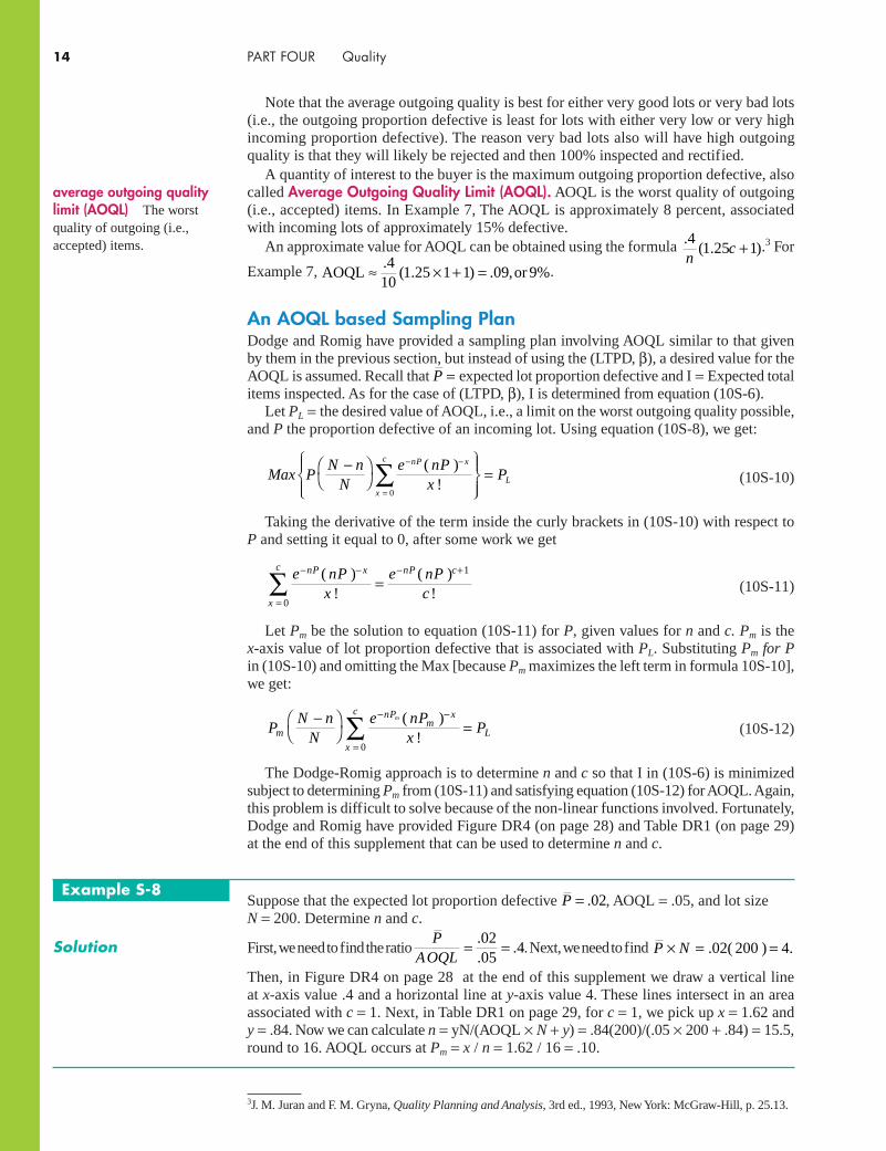
A quantity of interest to the buyer is the maximum outgoing proportion defective, also called Average outgoing Quality limit (AoQl). AOQL is the worst quality of outgoing (i.e., accepted) items. In Example 7, The AOQL is approximately 8 percent, associated with incoming lots of approximately 15% defective.
An approximate value for AOQL can be obtained using the formula .( . )
41 25 1
nc + .3 For
Example 7, AOQL or≈ × + =.( . ) . , %
410
1 25 1 1 09 9 .
An AoQl based Sampling planDodge and Romig have provided a sampling plan involving AOQL similar to that given by them in the previous section, but instead of using the (LTPD, β), a desired value for the AOQL is assumed. Recall that P = expected lot proportion defective and I = Expected total items inspected. As for the case of (LTPD, β), I is determined from equation (10S-6).
Let PL = the desired value of AOQL, i.e., a limit on the worst outgoing quality possible, and P the proportion defective of an incoming lot. Using equation (10S-8), we get:
Max PN n
Ne nP
xP
nP x
x
c
L
−
=
− −
=∑ ( )
!0
(10S-10)
Taking the derivative of the term inside the curly brackets in (10S-10) with respect to P and setting it equal to 0, after some work we get
e nPx
e nPc
nP x
x
c nP c− −
=
− +
∑ =( )!
( )!
0
1
(10S-11)
Let Pm be the solution to equation (10S-11) for P, given values for n and c. Pm is the x-axis value of lot proportion defective that is associated with PL. Substituting Pm for P in (10S-10) and omitting the Max [because Pm maximizes the left term in formula 10S-10], we get:
PN n
Ne nP
xPm
nPm
x
x
c
L
m−
=
− −
=∑ ( )
!0
(10S-12)
The Dodge-Romig approach is to determine n and c so that I in (10S-6) is minimized subject to determining Pm from (10S-11) and satisfying equation (10S-12) for AOQL. Again, this problem is difficult to solve because of the non-linear functions involved. Fortunately, Dodge and Romig have provided Figure DR4 (on page 28) and Table DR1 (on page 29) at the end of this supplement that can be used to determine n and c.
average outgoing quality limit (AoQl) The worst quality of outgoing (i.e., accepted) items.
3 J. M. Juran and F. M. Gryna, Quality Planning and Analysis, 3rd ed., 1993, New York: McGraw-Hill, p. 25.13.
Suppose that the expected lot proportion defective P = .02, AOQL = .05, and lot size N = 200. Determine n and c.
First, we need to find the ratio P
AOQL= =.
..
0205
4. Next, we need to find P N× = =. ( ) .02 200 4
Then, in Figure DR4 on page 28 at the end of this supplement we draw a vertical line at x-axis value .4 and a horizontal line at y-axis value 4. These lines intersect in an area associated with c = 1. Next, in Table DR1 on page 29, for c = 1, we pick up x = 1.62 and y = .84. Now we can calculate n = yN/(AOQL × N + y) = .84(200)/(.05 × 200 + .84) = 15.5, round to 16. AOQL occurs at Pm = x / n = 1.62 / 16 = .10.
example s-8
Solution
SUPPLEMENT TO CHAPTER 10 Acceptance Sampling 15
Key termsacceptable quality level (AQL), 5acceptance sampling, 2average outgoing quality (AOQ), 12average outgoing quality limit (AOQL), 13consumer’s risk, 5
lot tolerance percent defective (LTPD), 5operating characteristic (OC) curve, 3producer’s risk, 5sampling plans, 2
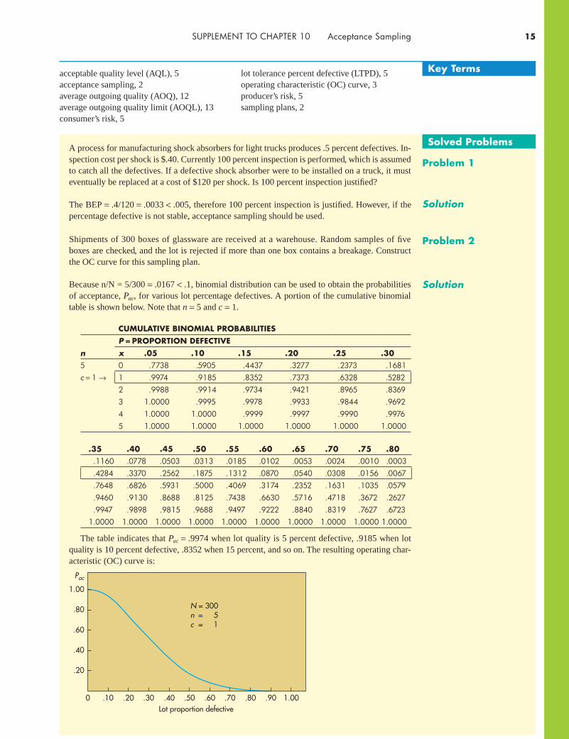
Problem 2Shipments of 300 boxes of glassware are received at a warehouse. Random samples of five boxes are checked, and the lot is rejected if more than one box contains a breakage. Construct the OC curve for this sampling plan.
solved ProblemsA process for manufacturing shock absorbers for light trucks produces .5 percent defectives. In-spection cost per shock is $.40. Currently 100 percent inspection is performed, which is assumed to catch all the defectives. If a defective shock absorber were to be installed on a truck, it must eventually be replaced at a cost of $120 per shock. Is 100 percent inspection justified?
SolutionBecause n/N = 5/300 = .0167 < .1, binomial distribution can be used to obtain the probabilities of acceptance, Pac, for various lot percentage defectives. A portion of the cumulative binomial table is shown below. Note that n = 5 and c = 1.
cUMULative binOMiaL PrObabiLitiesP = PrOPOrtiOn DeFective
n x .05 .10 .15 .20 .25 .305 0 .7738 .5905 .4437 .3277 .2373 .1681c = 1 → 1 .9974 .9185 .8352 .7373 .6328 .5282
2 .9988 .9914 .9734 .9421 .8965 .83693 1.0000 .9995 .9978 .9933 .9844 .96924 1.0000 1.0000 .9999 .9997 .9990 .99765 1.0000 1.0000 1.0000 1.0000 1.0000 1.0000
.35 .40 .45 .50 .55 .60 .65 .70 .75 .80.1160 .0778 .0503 .0313 .0185 .0102 .0053 .0024 .0010 .0003.4284 .3370 .2562 .1875 .1312 .0870 .0540 .0308 .0156 .0067.7648 .6826 .5931 .5000 .4069 .3174 .2352 .1631 .1035 .0579.9460 .9130 .8688 .8125 .7438 .6630 .5716 .4718 .3672 .2627.9947 .9898 .9815 .9688 .9497 .9222 .8840 .8319 .7627 .6723
1.0000 1.0000 1.0000 1.0000 1.0000 1.0000 1.0000 1.0000 1.0000 1.0000
The table indicates that Pac=.9974 when lot quality is 5 percent defective, .9185 when lot quality is 10 percent defective, .8352 when 15 percent, and so on. The resulting operating char-acteristic (OC) curve is:
Lot proportion defective.10 .20 .40 .50 .60
N = 300n = 5c = 1
1.00
.80
.60
.40
.20
Pac
.80 .900 .30 .70 1.00
Problem 1
SolutionThe BEP = .4/120 = .0033 < .005, therefore 100 percent inspection is justified. However, if the percentage defective is not stable, acceptance sampling should be used.

PART FOUR Quality16
Develop the AOQ curve for the previous problem using formula 10S-9.
What is acceptance sampling and what is its purpose? (LO1)1.
How does acceptance sampling differ from process control using control charts? (LO1)2.
When should a buyer use sampling inspection vs. 100% inspection vs. no inspection? 3. (LO1)
What general factors govern the choice between single-sampling and multiple-sampling plans? 4. (LO1)
What is an operating characteristic curve, and how is it useful in acceptance sampling? 5. (LO2)
Briefly explain or define each of these terms. (LO2)6.
AQL.a.
LTPD.b.
Producer’s risk.c.
Consumer’s risk.d.
When can each of the following distributions be used in calculating the probability of accep-7. tance of a lot? (LO2)
Hyper-geometric.a.
Binomial.b.
Poisson.c.
Discussion and review Questions
Problem 3
Solution AOQ = Pac × p
(Values of probability of acceptance Pac, can be taken from the top portion of the binomial table shown on the previous page)
Incoming proportion defective, p
.16
.12
.08
.04
0 .1 .2 .3 .4 .5 .6 .7 .8
Max = .158
AO
Q(O
utgo
ing
prop
ortio
n de
fect
ive)
p Pac aOQ p Pac aOQ
.05 .9974 .050 .45 .2562 .115
.10 .9185 .092 .50 .1875 .094
.15 .8352 .125 .55 .1312 .072
.20 .7373 .147 .60 .0870 .052
.25 .6328 .158 .65 .0540 .035
.30 .5258 .158 .70 .0380 .027
.35 .4284 .150 .75 .0156 .012
.40 .3370 .135 .80 .0067 .005

SUPPLEMENT TO CHAPTER 10 Acceptance Sampling 17
Visit http://www.itl.nist.gov/div898/handbook/pmc/section2/pmc22.htm, read about (a) 1. sequential, and (b) skip lot sampling plans, and define or explain them. (LO1)
Visit http://www.astm.org/SNEWS/JF_2010/datapoints_jf10.html, and summarize why we 2. still need Acceptance Sampling (given the existence of control charts). (LO1)
internet exercises
An assembly operation for the trigger mechanism of a semiautomatic spray gun produces a 1. small percentage of defective mechanisms. Management must decide whether to continue the current practice of 100 percent inspection, perform acceptance sampling, or replace defective mechanisms after final assembly when all guns are inspected. Replacement at final assembly costs $30 each; inspection during trigger assembly costs $12 per hour for labour and overhead. The inspection rate is one trigger per minute. (LO1)
Would 100 percent inspection during trigger assembly be justified if there are (1) 4 percent a. defective? (2) 1 percent defective?
At what point would management prefer acceptance sampling?b.
Random samples of 2. n = 20 circuit breakers are tested for damage caused by shipment in each lot of 4,000 received. Lots with more than one defective are pulled and subjected to 100 percent inspection. (LO2 & 4)
Construct the OC curve for this sampling plan.a.
Construct the AOQ curve for this plan using formula 10S-9, assuming defectives found b. during 100 percent inspection are replaced with good parts. What is the approximate AOQL?
Auditors use a technique called 3. discovery sampling in which a random sample of items is inspected. If any defects are found, the entire lot is subjected to 100 percent inspection. (LO2 & 4)
Draw an OC curve for the case where a sample of 15 credit accounts will be inspected out a. of a total of 8,000 accounts.
Draw an OC curve for the case where 150 accounts out of 8,000 accounts will be examined. b. (Hint: Use p = .001, .002, .003, . . .)
Draw the AOQ curve for the preceding case (part b), and determine the approximate c. AOQL.
Random samples of lots of textbooks are inspected for defective books just prior to shipment 4. to the publisher’s warehouse. Each lot contains 3,000 books. (LO2)
On a single graph, construct OC curves for a. n = 100 and (1) c = 0, (2) c = 1, and (3) c = 2. (Hint: Use p = .001, .002, .003, . . .)
On a single graph, construct OC curves for b. c = 2 and (1) n = 5, (2) n = 20, and (3) n = 120.
A manufacturer receives shipments of several thousand parts from a supplier every week. The 5. manufacturer has the option of inspection before accepting the parts. Inspection cost is $1 per unit. If parts are not inspected, defectives become apparent during a later assembly operation, at which time replacement cost is $6.25 per unit. (LO1 & 2)
At what proportion defective would the manufacturer prefer acceptance sampling?a.
For the sample size b. n = 15, what acceptance number c would result in probability of accep-tance close to .95 for AQL = 2%?
Problems
When would you use each of the four methods given in this supplement for determining single 8. sampling plans? (LO3)
Explain or define each of the following: (LO4)9.
AOQ.a.
AOQL.b.

PART FOUR Quality18
If the shipment actually contains 1 percent defective items and AQL c. =2 percent:
What is the correct decision?i.
What is the probability that the lot would be accepted if acceptable number ii. c = 0?
What is the probability that it would be rejected if iii. c = 0?
Answer the questions in part iv. c for a shipment that contains 3 percent defective items.
Suppose there are two defective units in a sample. (LO2 & 4)6.
If the acceptance number is a. c = 1, what decision should be made? What type of error is possible?
If the acceptance number is b. c = 3, what decision should be made? What type of error is possible?
Use formula 10S-9 to determine the average outgoing quality for each of the following c. percent defectives if c = 1 and n =15.
5 percent.i.
10 percent.ii.
15 percent.iii.
20 percent.iv.
Suppose lot size 7. N is 432 and acceptable quality level AQL is .65 percent. We would like to use Normal inspection at general inspection level II. Determine the sample size n and acceptance number c using MIL-STD-105E.4 (LO3)
A manufacturer of colour TV picture tubes is wondering if its current sampling procedure can 8. be improved.5 Currently, the defects are classified into critical (C: e.g., contaminated anode), major (B: e.g., bent pins) and minor (A: e.g., wrong label). The company has also grouped its customers into three groups and has one plan for each group: (LO3)
Existing Sampling Plans
Plan1 Plan2 Plan3
Nonconformity class C&B A C&B A C&B A
Lot size (N) 48 48 48 48 48 48
Documented AQL 1.0 1.0 2.5 2.5 2.5 2.5
Documented inspection severity Normal Reduced Reduced
Sample size (n) 8 8 5 5 3 3
Acceptance number (c) 0 1 1 1 0 0
For each plan and defect category, determine the sample size n and acceptance number c using MIL-STD-105E. Compare your results with the current plans above.
A single sampling plan uses sample size 9. n = 100 and the inspector accepts the lot if there are 2 or fewer defectives in the sample.6 You may use the Poisson approximation to answer the following questions. (LO2 & 4)
What is the probability of accepting a lot with proportion defective a. p = .01?
What protection does the buyer have against accepting lots with proportion defective b. p = .05?
What is the average outgoing quality AOQ for c. p = .01? Use formula 10S-9.
What is the average outgoing quality AOQ for d. p = .05? Use formula 10S-9.
4 E. F. Bauer, “A Move from Attribute to Variables Acceptance Sampling in an ISO-Certified Manufacturing Plant,” M.S. thesis, California State University, Dominguez Hills, 2000.
5 E. Gamino, “Improvement to the Acceptance Control System of a Manufacturer of Color Picture Tubes,” M.S. thesis, California State University, Dominguez Hills, 2005.
6 P. W. M. John, Statistical Methods in Engineering and Quality Assurance, New York: Wiley, 1990, p. 188.

SUPPLEMENT TO CHAPTER 10 Acceptance Sampling 19
What is the average outgoing quality limit AOQL for this plan? You may use the approxi-e.
mation .
( . )4
1 25 1n
c + .
*10. A manufacturer wishes to sample a purchased component used in its assembly operation.7 The company wishes to reject lots that are 5% defective. The components are received in lots of 1,000 units, which average 2.2% defective. The supplier has agreed to perform 100% inspection of all rejected lots. Find a sampling plan method that meets these conditions and determine n and c. (LO3)
*11. You are the quality manager for a company receiving large quantities of material from a sup-plier in lots of 1,000 units.8 The cost of inspecting the items is $.76 per unit. The cost of repair if bad material is introduced into your product is $15.20 per unit. A single sampling plan of 75 units with acceptance number of 2 has been suggested by one of your quality inspectors. In the past, lots submitted by this supplier have averaged 3.4% defective. (LO1–4)
a. Is acceptance sampling economically justified?
b. If you want to accept only lots of 4% defective or better, what do you think of the sampling plan of the inspector?
c. Suppose that rejected lots are 100% inspected. If a supplier submits many 4% defective lots, what will be the average outgoing quality of these lots? Use formula 10S-8.
12. a. Determine a sampling plan that will have AQL = 1% with producer risk α = .05 and LTPD = 5% with consumer risk β = .10.9 (LO3)
b. Suppose a sample is taken according to the sampling plan derived in part a and two non-conforming units are found. What action should be taken?
13. A housing development company buys heavy-duty nails in lots of 10,000 nails. A destruc-tive test is performed to determine the strength of the nails.10 AQL is 1% and LTPD is 10%. A single sample of n = 100 and c = 2 is used. Determine α and β. (LO3)
14. A manufacturer inspects all of its shipments to its customers prior to delivery using a double sampling MIL-STD-105E standard plan, Inspection level II, Normal type of inspection, and an AQL of 1%.11 The lot is 500 units. (LO3)
a. Find the sampling plan used and explain it in words.
b. Upon delivery of the product, the customer also inspects the lot using a single sampling MIL-STD-105E standard plan, AQL = 1.5%, inspection level II, and Normal type of inspec-tion. Find the customer’s sampling plan.
c. If a lot that is 10% defective is produced, calculate the probability that it will pass the manufacturer’s inspection.
d. Calculate the probability that a 10% defective lot will pass the customer’s inspection.
e. What is the probability that a 10% defective lot will pass both inspections?
15. Find the Dodge-Romig single sampling plan for AOQL = 4%, lot size of 125, and average lot percentage defective = 1%.12 (LO4)
16. Binder clips are packaged 12 to a box and 12 boxes to a carton.13 You have received a lot consisting of four cartons of binder clips. (LO3)
a. Use MIL-STD-105E to determine a single sampling plan to decide whether to accept or reject the lot. Use Inspection Level II, Normal type of inspection, and an AQL of 2.5%.
b. If in inspecting your sample you find three defective binder clips, what would you do?
7 J. M. Juran and F. M. Gryna, Quality Planning and Analysis, 3rd ed., 1993, New York: McGraw-Hill, p. 486.8 J. M. Juran and F. M. Gryna, Quality Planning and Analysis, 3rd ed, 1993, New York: McGraw-Hill, p. 487.9 J. M. Juran and F. M. Gryna, Juran’s Quality Control Handbook, 4th ed., 1988, New York: McGraw-Hill, pp. 25.26–25.27.
10 S. Nahmias, Production and Operations Analysis, 3rd ed., 1997, Chicago: Irwin.11 E. I. Grant and R. S. Leavenworth, Statistical Quality Control, 4th ed., 1972, New York: McGraw-Hill,
p. 445.12 E. G. Schilling, Acceptance Sampling in Quality Control, 1982, New York: Marcel Dekker, p. 398.13 http://www.shsu.edu/ ~ mgt_ves/mgt481/lesson9/lesson9.htm.

PART FOUR Quality20
Mini-case
gustave roussy InstituteAcceptance sampling is used in the Department of Clinical Pharmacy of Gustave Roussy Institute in Villejuif, France.15 Most of the over 10,000 custom-made units of 40 or so che-motherapy drugs produced during a semester (half year) for 5 semesters starting in 2001 were tested (at the cost of $1.50 each) to make sure that their content, dosage, and concentration were acceptable (i.e., within ±10% of the specification). Causes of defects were investigated and fixed so that percentage defec-tive was reduced from an average of 8.9% to 2.2%. Based on 50,000 test results, the test administrators classified the drugs into three classes:
category of Drugs Drugs concerned
Group 1 (17 drugs) <400 preparations a year
Irinotecan, oxaliplatin, gemcitabine, daunorubincin, idarubicin, fludarabine, melphalan, mitoxantrone, vindesine, vinorelbine, vinblastine, vincristine, dacarbazine, thiothepa, carboplatin, paclitaxel, docetaxel.
Group 2 (6 drugs) Acceptance sampling plan
Fluorouracil, ifosfamide, cisplatin, epirubicin, doxorubicin, cyclophosphamide
Group 3 (3 drugs) At risk to be outside the specification
Methotrexate, etoposide, cyarabine
Group 1 (17 drugs) were each issued less than 400 times a year. For this group it was decided to continue 100% inspection because the small number of issues during a semester may not be enough to be able to control their quality. Group 3 consisted of over 20% of production but the percentage defective of each (3 to 9%) was considered high enough to continue 100% inspec-tion. Group 2 (6 drugs) were considered to be candidates for acceptance sampling because their average percentage defective of 2.2% was stable and acceptable. For this group, AQL is 2.2% with α = .05 and LTPD is 5% with β = .05. Being cautious, the transition from 100% inspection into acceptance sampling is planned in stages. MIL-STD-105E tables are being used to deter-mine the sampling plans. The plans for one of the drugs are:
n c aQL LtPD
Fluorouracil
Observed 2484 67 2.22 3.16
Proposed sampling plans 2000 55 2.22 3.28
1500 43 2.25 3.50
1000 30 2.25 3.81
500 16 2.17 4.46
Calculate and comment on the assumed cost of a defective a. drug in Group 2 to a patient.
Determine the sample plan that should be used for Fluorou-b. racil and compare your plan with the proposed plans.
14 Y. Nikolaidis and G. Nenes, “Economic Evaluation of ISO 2859 Acceptance Sampling Plans Used with Rectifying Inspection of Rejected Lots,” Quality Engineering 21 (1), 2009, pp. 10–23.
15 I. Borget et al, “Application of an Acceptance Sampling Plan for Post-production Quality Control of Chemotherapeutic Batches in a Hospital Pharmacy,” European Journal of Pharmaceutics and Biopharmaceutics, 64 (2006), pp. 92–98.
Mini-case
cryStAl S.A.CRYSTAL S.A. is a Greek commercial fridge manufacturer.14 During packaging, CRYSTAL uses a wooden platform (pallet) under the fridge. The pallets use some wooden pegs (nogs). However, some nogs could be missing. The cost of inspecting a pallet is $.119. The average cost of putting nogs in pallets missing them is $.535 per pallet. If the defect is not identified before the pallet is used in packaging, it will cost $2.3 to take
the fridge off, insert the nogs in the pallet, and put the fridge back on the pallet. The pallets are bought in lot sizes of 800. The percentage of defective pallets in the past has ranged between 5 and 8%.
Questions
Should the company perform 100% inspection, acceptance a. sampling, or no inspection?
If acceptance sampling is best, what sampling plan should b. the company use? Justify your choice.

SUPPLEMENT TO CHAPTER 10 Acceptance Sampling 21
Px
cn x
PP
x
c
xn
x(
)(
)≤
=
−
=
−∑ 0
1
0
12
34
xc
= 1
cum
ulat
ive
bino
mia
l pro
babi
litie
s
P
nx
.05
.10
.15
.20
.25
.30
.35
.40
.45
.50
.55
.60
.65
.70
.75
.80
.85
.90
1. .
. .0
.950
0.9
000
.850
0.8
000
.750
0.7
000
.650
0.6
000
.550
0.5
000
.450
0.4
000
.350
0.3
000
.250
0.2
000
.150
0.1
000
11.
0000
1.00
001.
0000
1.00
001.
0000
1.00
001.
0000
1.00
001.
0000
1.00
001.
0000
1.00
001.
0000
1.00
001.
0000
1.00
001.
0000
1.00
002.
. . .
0.9
025
.810
0.7
225
.640
0.5
625
.490
0.4
225
.360
0.3
025
.250
0.2
025
.160
0.1
225
.090
0.0
625
.040
0.0
225
.010
01
.997
5.9
900
.977
5.9
600
.937
5.9
100
.877
5.8
400
.797
5.7
500
.697
5.6
400
.577
5.5
100
.437
5.3
600
.277
5.1
900
21.
0000
1.00
001.
0000
1.00
001.
0000
1.00
001.
0000
1.00
001.
0000
1.00
001.
0000
1.00
001.
0000
1.00
001.
0000
1.00
001.
0000
1.00
003.
. . .
0.8
574
.729
0.6
141
.512
0.4
219
.343
0.2
746
.216
0.1
664
.125
0.0
911
.064
0.0
429
.027
0.0
156
.008
0.0
034
.001
01
.992
8.9
720
.939
3.8
960
.843
8.7
840
.718
3.6
480
.574
8.5
000
.425
3.3
520
.281
8.2
160
.156
3.1
040
.060
8.0
280
2.9
999
.999
0.9
966
.992
0.9
844
.973
0.9
571
.936
0.9
089
.875
0.8
336
.784
0.7
254
.657
0.5
781
.488
0.3
859
.271
03
1.00
001.
0000
1.00
001.
0000
1.00
001.
0000
1.00
001.
0000
1.00
001.
0000
1.00
001.
0000
1.00
001.
0000
1.00
001.
0000
1.00
001.
0000
4. .
. .0
.814
5.6
561
.522
0.4
096
.316
4.2
401
.178
5.1
296
.091
5.0
625
.041
0.0
256
.015
0.0
081
.003
9.0
016
.000
5.0
001
1.9
860
.947
7.8
905
.819
2.7
383
.651
7.5
630
.475
2.3
910
.312
5.2
415
.179
2.1
265
.083
7.0
508
.027
2.0
120
.003
72
.999
5.9
963
.988
0.9
728
.949
2.9
163
.873
5.8
208
.758
5.6
875
.609
0.5
248
.437
0.3
483
.261
7.1
808
.109
5.0
523
31.
0000
.999
9.9
995
.998
4.9
961
.991
9.9
850
.974
4.9
590
.937
5.9
085
.870
4.8
215
.759
9.6
836
.590
4.4
780
.343
94
1.00
001.
0000
1.00
001.
0000
1.00
001.
0000
1.00
001.
0000
1.00
001.
0000
1.00
001.
0000
1.00
001.
0000
1.00
001.
0000
1.00
001.
0000
5. .
. .0
.773
8.5
905
.443
7.3
277
.237
3.1
681
.116
0.0
778
.050
3.0
313
.018
5.0
102
.005
3.0
024
.001
0.0
003
.000
1.0
000
1.9
974
.918
5.8
352
.737
3.6
328
.528
2.4
284
.337
0.2
562
.187
5.1
312
.087
0.0
540
.030
8.0
156
.006
7.0
022
.000
52
.998
8.9
914
.973
4.9
421
.896
5.8
369
.764
8.6
826
.593
1.5
000
.406
9.3
174
.235
2.1
631
.103
5.0
579
.026
6.0
086
31.
0000
.999
5.9
978
.993
3.9
844
.969
2.9
460
.913
0.8
688
.812
5.7
438
.663
0.5
716
.471
8.3
672
.262
7.1
648
.081
54
1.00
001.
0000
.999
9.9
997
.999
0.9
976
.994
7.9
898
.981
5.9
688
.949
7.9
222
.884
0.8
319
.762
7.6
723
.556
3.4
095
51.
0000
1.00
001.
0000
1.00
001.
0000
1.00
001.
0000
1.00
001.
0000
1.00
001.
0000
1.00
001.
0000
1.00
001.
0000
1.00
001.
0000
1.00
006.
. . .
0.7
351
.531
4.3
771
.262
1.1
780
.117
6.0
754
.046
7.0
277
.015
6.0
083
.004
1.0
018
.000
7.0
002
.000
1.0
000
.000
01
.967
2.8
857
.776
5.6
554
.533
9.4
202
.319
1.2
333
.163
6.1
094
.069
2.0
410
.022
3.0
109
.004
6.0
016
.000
4.0
001
2.9
978
.984
2.9
527
.901
1.8
306
.744
3.6
471
.544
3.4
415
.343
8.2
553
.179
2.1
174
.070
5.0
376
.017
0.0
059
.001
33
.999
9.9
987
.994
1.9
830
.962
4.9
295
.882
6.8
208
.744
7.6
563
.558
5.4
557
.352
9.2
557
.169
4.0
989
.047
3.0
159
41.
0000
.999
9.9
996
.998
4.9
954
.989
1.9
777
.959
0.9
308
.890
6.8
364
.766
7.6
809
.579
8.4
661
.344
6.2
235
.114
35
1.00
001.
0000
1.00
00.9
999
.999
8.9
993
.998
2.9
959
.991
7.9
844
.972
3.9
533
.924
6.8
824
.822
0.7
379
.622
9.4
686
61.
0000
1.00
001.
0000
1.00
001.
0000
1.00
001.
0000
1.00
001.
0000
1.00
001.
0000
1.00
001.
0000
1.00
001.
0000
1.00
001.
0000
1.00
007.
. . .
0.6
983
.478
3.3
206
.209
7.1
335
.082
4.0
490
.028
0.0
152
.007
8.0
037
.001
6.0
006
.000
2.0
001
.000
0.0
000
.000
01
.955
6.8
503
.716
6.5
767
.444
9.3
294
.233
8.1
586
.102
4.0
625
.035
7.0
188
.009
0.0
038
.001
3.0
004
.000
1.0
000

PART FOUR Quality22P
nx
.05
.10
.15
.20
.25
.30
.35
.40
.45
.50
.55
.60
.65
.70
.75
.80
.85
.90
2.9
962
.974
3.9
262
.852
0.7
564
.647
1.5
323
.419
9.3
164
.226
6.1
529
.096
3.0
556
.028
8.0
129
.004
7.0
012
.000
23
.999
8.9
973
.987
9.9
667
.929
4.8
740
.800
2.7
102
.608
3.5
000
.391
7.2
898
.199
8.1
260
.070
6.0
333
.012
1.0
027
41.
0000
.999
8.9
988
.995
3.9
871
.971
2.9
444
.903
7.8
471
.773
4.6
836
.580
1.4
677
.352
9.2
436
.148
0.0
738
.025
75
1.00
001.
0000
.999
9.9
996
.998
7.9
962
.991
0.9
812
.964
3.9
375
.897
6.8
414
.766
2.6
706
.555
1.4
233
.283
4.1
497
61.
0000
1.00
001.
0000
1.00
00.9
999
.999
8.9
994
.998
4.9
963
.992
2.9
848
.972
0.9
510
.917
6.8
665
.790
3.6
794
.521
77
1.00
001.
0000
1.00
001.
0000
1.00
001.
0000
1.00
001.
0000
1.00
001.
0000
1.00
001.
0000
1.00
001.
0000
1.00
001.
0000
1.00
001.
0000
8. .
. .0
.663
4.4
305
.272
5.1
678
.100
1.0
576
.031
9.0
168
.008
4.0
039
.001
7.0
007
.000
2.0
001
.000
0.0
000
.000
0.0
000
1.9
428
.813
1.6
572
.503
3.3
671
.255
3.1
691
.106
4.0
632
.035
2.0
181
.008
5.0
036
.001
3.0
004
.000
1.0
000
.000
02
.994
2.9
619
.894
8.7
969
.678
5.5
518
.427
8.3
154
.220
1.1
445
.088
5.0
498
.025
3.0
113
.004
2.0
012
.000
2.0
000
3.9
996
.995
0.9
786
.943
7.8
862
.805
9.7
064
.594
1.4
470
.363
3.2
604
.173
7.1
061
.058
0.0
273
.010
4.0
029
.000
44
1.00
00.9
996
.997
1.9
896
.972
7.9
420
.893
9.8
263
.739
6.6
367
.523
0.4
059
.293
6.1
941
.113
8.0
563
.021
4.0
050
51.
0000
1.00
00.9
998
.998
8.9
958
.988
7.9
747
.950
2.9
115
.855
5.7
799
.684
8.5
722
.448
2.3
215
.203
1.1
052
.038
16
1.00
001.
0000
1.00
00.9
999
.999
6.9
987
.996
4.9
915
.981
9.9
648
.936
8.8
936
.830
9.7
447
.632
9.4
967
.342
8.1
869
71.
0000
1.00
001.
0000
1.00
001.
0000
.999
9.9
998
.999
3.9
983
.996
1.9
916
.983
2.9
681
.942
4.8
999
.832
2.7
275
.569
58
1.00
001.
0000
1.00
001.
0000
1.00
001.
0000
1.00
001.
0000
1.00
001.
0000
1.00
001.
0000
1.00
001.
0000
1.00
001.
0000
1.00
001.
0000
9. .
. .0
.630
2.3
874
.231
6.1
342
.075
1.0
404
.020
7.0
101
.004
6.0
020
.000
8.0
003
.000
1.0
000
.000
0.0
000
.000
0.0
000
1.9
288
.774
8.5
995
.436
2.3
003
.196
0.1
211
.070
5.0
385
.019
5.0
091
.003
8.0
014
.000
4.0
001
.000
0.0
000
.000
02
.991
6.9
470
.859
1.7
382
.600
7.4
628
.337
3.2
318
.149
5.0
898
.049
8.0
250
.011
2.0
043
.001
3.0
003
.000
0.0
000
3.9
994
.991
7.9
661
.914
4.8
343
.729
7.6
089
.482
6.3
614
.253
9.1
658
.099
4.0
536
.025
3.0
100
.003
1.0
006
.000
14
1.00
00.9
991
.994
4.9
804
.951
1.9
012
.828
3.7
334
.621
4.5
000
.378
6.2
666
.171
7.0
988
.048
9.0
196
.005
6.0
009
51.
0000
.999
9.9
994
.996
9.9
900
.974
7.9
464
.900
6.8
342
.746
1.6
386
.517
4.3
911
.270
3.1
657
.085
6.0
339
.008
36
1.00
001.
0000
1.00
00.9
997
.998
7.9
957
.988
8.9
750
.950
2.9
102
.850
5.7
682
.662
7.5
372
.399
3.2
618
.140
9.0
530
71.
0000
1.00
001.
0000
1.00
00.9
999
.999
6.9
986
.996
2.9
909
.980
5.9
615
.929
5.8
789
.804
0.6
997
.563
8.4
005
.225
28
1.00
001.
0000
1.00
001.
0000
1.00
001.
0000
.999
9.9
997
.999
2.9
980
.995
4.9
899
.979
3.9
596
.924
9.8
658
.768
4.6
126
91.
0000
1.00
001.
0000
1.00
001.
0000
1.00
001.
0000
1.00
001.
0000
1.00
001.
0000
1.00
001.
0000
1.00
001.
0000
1.00
001.
0000
1.00
0010
. . .
.0
.598
7.3
487
.196
9.1
074
.056
3.0
282
.013
5.0
060
.002
5.0
010
.000
3.0
001
.000
0.0
000
.000
0.0
000
.000
0.0
000
1.9
139
.736
1.5
443
.375
8.2
440
.149
3.0
860
.046
4.0
233
.010
7.0
045
.001
7.0
005
.000
1.0
000
.000
0.0
000
.000
02
.988
5.9
298
.820
2.6
778
.525
6.3
828
.261
6.1
673
.099
6.0
547
.027
4.0
123
.004
8.0
016
.000
4.0
001
.000
0.0
000
3.9
990
.987
2.9
500
.879
1.7
759
.649
6.5
138
.382
3.2
660
.171
9.1
020
.054
8.0
260
.010
6.0
035
.000
9.0
001
.000
04
.999
9.9
984
.990
1.9
672
.921
9.8
497
.751
5.6
331
.504
4.3
770
.261
6.1
662
.094
9.0
473
.019
7.0
064
.001
4.0
001
51.
0000
.999
9.9
986
.993
6.9
803
.952
7.9
051
.833
8.7
384
.623
0.4
956
.366
9.2
485
.150
3.0
781
.032
8.0
099
.001
66
1.00
001.
0000
.999
9.9
991
.996
5.9
894
.974
0.9
452
.898
0.8
281
.734
0.6
177
.486
2.3
504
.224
1.1
209
.050
0.0
128
71.
0000
1.00
001.
0000
.999
9.9
996
.998
4.9
952
.987
7.9
726
.945
3.9
004
.832
7.7
384
.617
2.4
744
.322
2.1
798
.070
28
1.00
001.
0000
1.00
001.
0000
1.00
00.9
999
.999
5.9
983
.995
5.9
893
.976
7.9
536
.914
0.8
507
.756
0.6
242
.455
7.2
639
91,
0000
1.00
001.
0000
1.00
001.
0000
1.00
001.
0000
.999
9.9
997
.999
0.9
975
.994
0.9
865
.971
8.9
437
.892
6.8
031
.651
310
1.00
001.
0000
1.00
001.
0000
1.00
001.
0000
1.00
001.
0000
1.00
001.
0000
1.00
001.
0000
1.00
001.
0000
1.00
001.
0000
1.00
001.
0000
15. .
. .
0.4
633
.205
9.0
874
.035
2.0
134
.004
7.0
016
.000
5.0
001
.000
0.0
000
.000
0.0
000
.000
0.0
000
.000
0.0
000
.000
0

SUPPLEMENT TO CHAPTER 10 Acceptance Sampling 23
P
nx
.05
.10
.15
.20
.25
.30
.35
.40
.45
.50
.55
.60
.65
.70
.75
.80
.85
.90
1.8
290
.549
0.3
186
.167
1.0
802
.035
3.0
142
.005
2.0
017
.000
5.0
001
.000
0.0
000
.000
0.0
000
.000
0.0
000
.000
02
.963
8.8
159
.604
2.3
980
.236
1.1
268
.061
7.0
271
.010
7.0
037
.001
1.0
003
.000
1.0
000
.000
0.0
000
.000
0.0
000
3.9
945
.944
4.8
227
.648
2.4
613
.296
9.1
727
.090
5.0
424
.017
6.0
063
.001
9.0
005
.000
1.0
000
.000
0.0
000
.000
04
.999
4.9
873
.938
3.8
358
.686
5.5
155
.351
9.2
173
.120
4.0
592
.025
5.0
093
.002
8.0
007
.000
1.0
000
.000
0.0
000
5.9
999
.997
8.9
832
.938
9.8
516
.721
6.5
643
.403
2.2
608
.150
9.0
769
.033
8.0
124
.003
7.0
008
.000
1.0
000
.000
06
1.00
00.9
997
.996
4.9
819
.943
4.8
689
.754
8.6
098
.452
2.3
036
.181
8.0
950
.042
2.0
152
.004
2.0
008
.000
1.0
000
71.
0000
1.00
00.9
994
.995
8.9
827
.950
0.8
868
.786
9.6
535
.500
0.3
465
.213
1.1
132
.050
0.0
173
.004
2.0
006
.000
08
1.00
001.
0000
.999
9.9
992
.995
8.9
848
.957
8.9
050
.818
2.6
964
.547
8.3
902
.245
2.1
311
.056
6.0
181
.003
6.0
003
91.
0000
1.00
001.
0000
.999
9.9
992
.996
3.9
876
.966
2.9
231
.849
1.7
392
.596
8.4
357
.278
4.1
484
.061
1.0
168
.002
210
1.00
001.
0000
1.00
001.
0000
.999
9.9
993
.997
2.9
907
.974
5.9
408
.879
6.7
827
.648
1.4
845
.313
5.1
642
.061
7.0
127
111.
0000
1.00
001.
0000
1.00
001.
0000
.999
9.9
995
.998
1.9
937
.982
4.9
576
.909
5.8
273
.703
1.5
387
.351
8.1
773
.055
612
1.00
001.
0000
1.00
001.
0000
1.00
001.
0000
.999
9.9
997
.998
9.9
963
.989
3.9
729
.938
3.8
732
.763
9.6
020
.395
8.1
841
131.
0000
1.00
001.
0000
1.00
001.
0000
1.00
001.
0000
1.00
00.9
999
.999
5.9
983
.994
8.9
858
.964
7.9
198
.832
9.6
814
.451
014
1.00
001.
0000
1.00
001.
0000
1.00
001.
0000
1.00
001.
0000
1.00
001.
0000
.999
9.9
995
.998
4.9
953
.986
6.9
648
.912
6.7
941
151.
0000
1.00
001.
0000
1.00
001.
0000
1.00
001.
0000
1.00
001.
0000
1.00
001.
0000
1.00
001.
0000
1.00
001.
0000
1.00
001.
0000
1.00
0020
. . .
.0
.358
5.1
216
.038
8.0
115
.003
2.0
008
.000
2.0
000
.000
0.0
000
.000
0.0
000
.000
0.0
000
.000
0.0
000
.000
0.0
000
1.7
358
.391
7.1
756
.069
2.0
243
.007
6.0
021
.000
5.0
001
.000
0.0
000
.000
0.0
000
.000
0.0
000
.000
0.0
000
.000
02
.924
5.6
769
.404
9.2
061
.091
3.0
355
.012
1.0
036
.000
9.0
002
.000
0.0
000
.000
0.0
000
.000
0.0
000
.000
0.0
000
3.9
841
.867
0.6
477
.411
4.2
252
.107
1.0
444
.016
0.0
049
.001
3.0
003
.000
0.0
000
.000
0.0
000
.000
0.0
000
.000
04
.997
4.9
568
.829
8.6
296
.414
8.2
375
.118
2.0
510
.018
9.0
059
.001
5.0
003
.000
0.0
000
.000
0.0
000
.000
0.0
000
5.9
997
.988
7.9
327
.804
2.6
172
.416
4.2
454
.125
6.0
553
.020
7.0
064
.001
6.0
003
.000
0.0
000
.000
0.0
000
.000
06
1.00
00.9
976
.978
1.9
133
.785
8.6
080
.416
6.2
500
.129
9.0
577
.021
4.0
065
.001
5.0
003
.000
0.0
000
.000
0.0
000
71.
0000
.999
6.9
941
.967
9.8
982
.772
3.6
010
.415
9.2
520
.131
6.0
580
.021
0.0
060
.001
3.0
002
.000
0.0
000
.000
08
1.00
00.9
999
.998
7.9
900
.959
1.8
867
.762
4.5
956
.414
3.2
517
.130
8.0
565
.019
6.0
051
.000
9.0
001
.000
0.0
000
91.
0000
1.00
00.9
998
.997
4.9
861
.952
0.8
782
.755
3.5
914
.411
9.2
493
.127
5.0
532
.017
1.0
039
.000
6.0
000
.000
010
1.00
001.
0000
1.00
00.9
994
.996
1.9
829
.946
8.8
725
.750
7.5
881
.408
6.2
447
.121
8.0
480
.013
9.0
026
.000
2.0
000
111.
0000
1.00
001.
0000
.999
9.9
991
.994
9.9
804
.943
5.8
692
.748
3.5
857
.404
4.2
376
.113
3.0
409
.010
0.0
013
.000
112
1.00
001.
0000
1.00
001.
0000
.999
8.9
987
.994
0.9
790
.942
0.8
684
.748
0.5
841
.399
0.2
277
.101
8.0
321
.005
9.0
004
131.
0000
1.00
001.
0000
1.00
001.
0000
.999
7.9
985
.993
5.9
786
.942
3.8
701
.750
0.5
834
.392
0.2
142
.086
7.0
219
.002
414
1.00
001.
0000
1.00
001.
0000
1.00
001.
0000
.999
7.9
984
.993
6.9
793
.944
7.8
744
.754
6.5
836
.382
8.1
958
.067
3.0
113
151.
0000
1.00
001.
0000
1.00
001.
0000
1.00
001.
0000
.999
7.9
985
.994
1.9
811
.949
0.8
818
.762
5.5
852
.370
4.1
702
.043
216
1.00
001.
0000
1.00
001.
0000
1.00
001.
0000
1.00
001.
0000
.999
7.9
987
.995
1.9
840
.955
6.8
929
.774
8.5
886
.352
3.1
330
171.
0000
1.00
001.
0000
1.00
001.
0000
1.00
001.
0000
1.00
001.
0000
.999
8.9
991
.996
4.9
879
.964
5.9
087
.793
9.5
951
.323
118
1.00
001.
0000
1.00
001.
0000
1.00
001.
0000
1.00
001.
0000
1.00
001.
0000
.999
9.9
995
.997
9.9
924
.975
7.9
308
.824
4.6
083
191.
0000
1.00
001.
0000
1.00
001.
0000
1.00
001.
0000
1.00
001.
0000
1.00
001.
0000
1.00
00.9
998
.999
2.9
968
.988
5.9
612
.878
420
1.00
001.
0000
1.00
001.
0000
1.00
001.
0000
1.00
001.
0000
1.00
001.
0000
1.00
001.
0000
1.00
001.
0000
1.00
001.
0000
1.00
001.
0000

PART FOUR Quality24
Larson’s Binomial Nomograph
.010 1000
Number of trials or sample size (n)
700500
400300
200140
10070
5040
3020
20
1
23
45
Occ
urre
nces
(c)
79
102030405070100140
10
5
5
10
20
Num
ber o
f occ
urre
nces
(c)
40
5070
100
140
200
.02
.03
.04
.05
.06
.07
.08
.09
.10
Prob
abili
ty o
f occ
urre
nce
in a
sin
gle
trial
(p)
.15
.20
.25
.30
.35
.40
.45
.50
.001.10.02
.08.95
n = 90
nN
c = 3
.005
.01
.02
.05
.10
.20
.30
.40
Prob
abili
ty o
f c o
r few
er o
ccur
renc
es in
n tr
ials
(P)
.50
.60
.70
.80
.90
.95
.98
.99
.995
.999
pP
P = P{m � c} = pm(1 – p)n – m c
m = 0� n!
m!(n – m)!
� 0.1

SUPPLEMENT TO CHAPTER 10 Acceptance Sampling 25
Ratio of process average to tolerance[P/Pt = (Process average fraction defective)/(Tolerance fraction defective)]
Accep
tance
numbe
r
1000
800
600
500
400
300
200
100
80
6050
40
30
20
10 0
1
2
3
5
6
7
891011
12
13
14
15
16
17
18
1920
25
ToTo
To
3021
26
35
31
4
8
65
4
3
2
10 0.1 0.2 0.3 0.4 0.5 0.6
Single samplingconsumer’s risk, 0.10
Tole
ranc
e nu
mbe
r of d
efec
tives
[PtN
= (T
oler
ance
frac
tion
defe
ctiv
e) (L
ot s
ize)
]
Figure DR1 Dodge-Romig Curves for Finding the Acceptance Number
Source: H. F. Dodge and H. G. Romig, Sampling Inspection Tables, 2nd ed, 1959, New York: John Wiley, p. 14.

PART FOUR Quality26
24
22
20
18
16
Tole
ranc
e tim
es s
ampl
e siz
e[P
tn =
(Tol
eran
ce fr
actio
n de
fect
ive)
(Sam
ple
size)
]
14
12
10
8
6
4
2
01 2 3 4 5 7 10 20
Tolerance number of defectives[PtN = (Tolerance fraction defective) (Lot size)]
30 50 70 100 200 300 500 1000
01 2
3 45
67
8910
111213141516171819
Simple samplingconsumers risk, O.IO
Acce
ptan
ce n
umbe
r
Figure DR2 Dodge-Romig Curves for Finding the Size of Sample
Source: H. F. Dodge and H. G. Romig, Sampling Inspection Tables, 2nd ed, 1959, New York: John Wiley, p. 15.

SUPPLEMENT TO CHAPTER 10 Acceptance Sampling 27
1000
800
600
500
400
300
200
100
80
60
50
40
30
20
10
8
6
5
4
3
2
0 0.1 0.2 0.3 0.4 0.5 0.6
1.5
2
3
4
5
6
78
91011
1315
20
25
30
35
40
1
Single samplingconsumer’s risk, 0.10
Ratio of process average to tolerance[P/Pt = (Process average fraction defective)/(Tolerance fraction defective)]
Tole
ranc
e nu
mbe
r of d
efec
tives
[PtN
= (T
oler
ance
frac
tion
defe
ctiv
e) (L
ot s
ize)
]
Tole
ranc
e tim
es m
inim
um a
vera
ge in
spec
ted
[PtI m
in =
(Tol
eran
ce fr
actio
n de
fect
ive)
(Min
imum
ave
rage
num
ber i
nspe
cted
per
lot)]
Figure DR3 Dodge-Romig Curves for Finding the Minimum Amount of Inspection per Lot
Source: H. F. Dodge and H. G. Romig, Sampling Inspection Tables, 2nd ed, 1959, New York: John Wiley, p. 16.

PART FOUR Quality28
10 0008000
600050004000
3000
2000
1000800
600500400
300
200
10080
605040
30
20
108
654
3
2
C = 0
1
2
3
4
10 0.1 0.2 0.3 0.4 0.5 0.6 0.7 0.8 0.9 1.0 1.1 1.2 1.3 1.4 1.5
k = (ratio of process average fraction defective to AOQL)ppL
M =
pN
(pro
cess
ave
rage
frac
tion
defe
ctiv
e tim
es lo
t siz
e)
5
6
78910
121416
18
20
21 to
2515
C
17
19
Figure DR4 Dodge-Romig Curves for Determining the Acceptance Number c; AOQL Protection
Source: H. F. Dodge and H. G. Romig, Sampling Inspection Tables, 1944, New York: John Wiley, p. 50.

SUPPLEMENT TO CHAPTER 10 Acceptance Sampling 29
given c x y given c x y given c x y given c x y
0 1.00 0.3679 10 8.05 6.528 20 15.92 13.89 30 24.11 21.70
1 1.62 0.8400 11 8.82 7.233 21 16.73 14.66 31 24.95 22.50
2 2.27 1.371 12 9.59 7.948 22 17.54 15.43 32 25.78 23.30
3 2.95 1.942 13 10.37 8.670 23 18.35 16.20 33 26.62 24.10
4 3.64 2.544 14 11.15 9.398 24 19.17 16.98 34 27.45 24.90
5 4.35 3.168 15 11.93 10.13 25 19.99 17.76 35 28.29 25.71
6 5.07 3.812 16 12.72 10.88 26 20.81 18.54 36 29.13 26.52
7 5.80 4.472 17 13.52 11.62 27 21.63 19.33 37 29.97 27.33
8 6.55 5.146 18 14.31 12.37 28 22.46 20.12 38 30.82 28.14
9 7.30 5.831 19 15.12 13.13 29 23.29 20.91 39 31.66 28.96
10 8.05 6.528 20 15.92 13.89 30 24.11 21.70 40 32.51 29.77
Table DR1 Dodge-Romig values of x and y for Determining AOQL
Source: H. F. Dodge and H. G. Romig, Sampling Inspection Tables, 1944, New York: John Wiley, p. 49.