Page 1 of 1

Neuron, Volume 81

Supplemental Information

Comparison of Human Ventral Frontal Cortex Areas

for Cognitive Control and Language

with Areas in Monkey Frontal Cortex

Franz-Xaver Neubert, Rogier B. Mars, Adam G. Thomas, Jerome Sallet, and Matthew F.S.

Rushworth

1

Supplemental Information for “Comparison of human frontal cortex areas for

cognitive control and language with areas in monkey frontal cortex”

Supplemental Experimental Procedures and Results

(1) Diffusion-weighted MRI data acquisition

Diffusion-weighted images were acquired in 25 healthy right-handed (according to Edinburgh Handedness Inventory:

mean +/- SD, 77 +/- 26.7) participants (14 female; age range: 20 – 45 years; mean age +/- SD, 29 +/- 6.6 years) on a 3

T Siemens Magnetom Verio MR scanner.

All participants gave written informed consent in accordance with ethical approval from the local ethics committee.

Participants lay supine in the scanner, and cushions were used to reduce head motion. Diffusion-weighted data were

acquired using echo planar imaging (65 2.0 mm thick axial slices; field of view, 190 x 190 mm2; and a voxel size of 2 x

2 x 2 mm). Diffusion weighting was isotropically distributed along 60 directions using a b-value of 1.000 s×mm-2.

Eight volumes with no diffusion weighting were acquired throughout the acquisition. A structural scan was acquired

for each participant in the same session, using a T1-weighted three-dimensional fast, low-angle shot (3D Multiecho

MPRAGE) sequence [repetition time (TR), 2530 ms; echo time (TE), 1.69 ms; flip angle, 7.0 °; with elliptical sampling

of k space, giving voxel size of 1.0 x 1.0 x 1.0 mm].

(2) Diffusion-weighted tractography-based parcellation

DW-MRI data were pre-processed using tools from FDT v2.0 (FMRIB’s Diffusion Toolbox; part of FSL 4.1). Eddy-

current-distortions were corrected using affine registration of all volumes to a target volume with no diffusion

weighting. EPI unwarping was performed using FMRIB's Utility for Geometrically Unwarping EPIs v2.5 (FUGUE).

Voxel-wise estimates of the fibre orientation distribution were calculated using Bedpostx, limited to estimating two

fibre orientations at each voxel, because of the b-value and number of gradient orientations in the diffusion data

(Behrens et al., 2007).

The vlFC ROI was registered from the MNI152 template brain as provided by FSL to the individual subject’s T1-

weighted structural image using FNRIT (FMRIB's Non-linear Image Registration Tool) and then registered from the

individual subject’s structural image into the individual subject’s DW-MRI space using FLIRT (FMRIB's Linear Image

Registration Tool). For each participant, probabilistic tractography was run from each voxel in the right vlFC ROI to

generate a connectivity matrix between all vlFC voxels and each brain voxel as described (Johansen-Berg et al., 2004)

and used to generate a symmetric cross-correlation matrix for all vlFC voxels. This cross-correlation matrix was then

permuted using k-means segmentation for automated clustering to define different clusters. K-means can be

sensitive to initialisation, but there are some ways to minimize these effects. In the implementation of k-means used

here (“ccops” as implemented in FSL), starting points are chosen as follows: a random point is chosen to be the first

cluster centre, then the second cluster centre is the point furthest from the first one, the third the point furthest

from the average of the first two, etc until k centres are obtained. Thus, the only randomness lies in the position of

the first cluster center starting point. Additionally we clustered the seed voxels in the cross correlation matrix using

the fuzzy k-means algorithm. This algorithm, rather than just assigning each voxel in the vlFC seed ROI to one of the

clusters, also gives a certainty of each voxel belonging to each of the clusters and hence provides a “certainty map”

of the whole vlFC ROI for each cluster. The clusters were then all registered to the MNI152 template by inverting the

linear (DW-MRI to T1-weighted structural image) and non-linear (T1-weighted structural image to MNI152_2mm

template as provided by FSL) registration matrices / warp-fields that were used before and then matched between

subjects for spatial overlap.

2

(3) Number of clusters of the diffusion-weighted tractography-based parcellation

To determine the optimal number of clusters resulting in consistency across participants as well as coherency within

the individual participants, we divided the right vlFC into clusters ranging from two to 25. We emphasize that the

goal of this vlFC parcellation into vlFC sub-regions with coherent structural connectivity was not to determine exactly

how many sub-regions there are in the vlFC. Such claims can hardly be tenable not only because of the limitations

imposed by quality and resolution of the imaging data but also because they depend on what definition of “brain

area” is used. Rather, the goal of this study is to test the hypothesis that different sub-regions in the vlFC can reliably

be found and that the different structural and functional connectivity of these sub-regions might allow them to exert

different types of top-down control onto other brain regions during a variety of cognitive tasks, such as language or

cognitive control tasks. Hence the connectivity-based parcellation was limited to identifying sub-regions that are

consistent within the group of subjects and then also found to be consistent in a second group of subjects. Similar

inter-subject consistency in signal location is a prerequisite for most functional neuroimaging studies.

To ensure that the clustering procedure yields a sensible, reliable and robust parcellation of the vlFC we carried out a

series of analyses that each attempted to parcellate vlFC into different numbers of sub-regions. We clustered the

probabilistic tracking results into two to 25 clusters and analysed the results in the following way: First, we

calculated the average cross-correlation value in the cross correlation matrix for each cluster in each subject

(normalised for the overall cross correlation value in the cross correlation matrix) and calculated the variance of

these cluster specific cross correlation values for each clustering solution. It is of course the case that the average

cross correlation in each cluster increases as the number of clusters increases and the highest possible average cross

correlation value would be reached with a clustering into as many clusters as there are voxels in the ROI. However,

we do not expect there to be as many clusters as there are voxels in the vlFC. Within the range of two to 25 clusters

a low variance of the average cross correlation should indicate a coherent clustering into similarly correlated clusters

without very well or very poorly correlated outlier-clusters. The group average cross correlation values for each

cluster in the two to 25 clusters solutions is shown in Supplemental Figure 1B (in red diamonds) together with the

variance of the measures (in blue squares). This measure indicates that the ten cluster solution shows the smallest

variance in the average cross correlation and might therefore be considered as the solution that provides the most

coherent clustering into similarly correlated clusters without very well or very poorly correlated outlier-clusters.

Second, we looked at the spatial overlap between corresponding clusters across the 25 subjects for each of the two

to 25 clusters solutions. Supplemental Figure 1C shows in red triangles the average spatial overlap between

corresponding clusters across the 25 participants for the different clustering solutions. Two indices of overlap were

used. First, we examined the average degree of spatial overlap for a given cluster across all clusters (green dashed

line) and, second, the degree of spatial overlap for the cluster with the lowest spatial overlap (cyan dotted line). In

both cases parcellation solutions with ten vlFC subregions had maximal spatial overlaps (at least in the range of five

to 25 clusters).

Third, in order to cross-validate the vlFC parcellation, we looked at the spatial overlap between the vlFC sub-regions

derived from the two to 25 cluster solutions in the 25 participants on a group level with corresponding clusters in an

independent group of eight subjects (see Supplemental Figure 1D). This analysis was done to ensure that the

proposed vlFC parcellation that was based on a group of 25 subjects also holds true in other subjects. We also

wanted to see which of the two to 25 clusters clustering solutions on a group level were reliably replicable in an

independent group of subjects. Supplemental Figure1D shows with a red dashed line the average degree of spatial

overlap for a given cluster across all clusters and with a blue dotted line the degree of spatial overlap for the cluster

with the lowest spatial overlap. In both cases parcellation solutions with ten vlFC subregions had the maximal spatial

overlaps between the group of 25 participants and the independent group of eight subjects (at least in the range of

five to 25 clusters).

3

We also determined the centers of gravity for each of the clusters in each individual participant. Centres of gravity

for each of the clusters in each individual participant with ellipsoids representing the 95% confidence limits of the

mean group cluster location are plotted on the structural MNI brain for the ten cluster-parcellation (Supplemental

Figure 1E and F). Moreover the comparison of our parcellation derived functional connectivity results with functional

connectivity of various different cyto-architectonically defined regions in the macaque vlFC further corroborates the

plausibility of the parcellation of the vlFC into different sub-regions (for the between species comparison see below

SI.6).

It is apparent that an iterative parcellation procedure (see SI.4) yielded largely similar results to the ten cluster

parcellation. However using an iterative parcellation procedure it was also possible to further parcellate two of the

ten regions (a region that extended from the pars orbitalis to the deep frontal operculum was sub-parcellated into

lateral area 47 and the deep frontal operculum area Op; area 44 could be further sub-divided into a dorsal and a

ventral part: 44d and 44v).

(4) Recursive parcellation and sub-parcellation attempts

In addition to the ten cluster parcellation solution a recursive or iterative clustering procedure similar to the one

used by (Beckmann et al., 2009) was conducted. Supplementary Figure 2 illustrates this procedure and shows the

results. The parcellation started with the exact same vlFC ROI (leftmost image in SFig. 2) and was conducted in the

same 25 subjects. Probabilistic tractography from each voxel in the ROI was used to parcellate the whole ROI into

two sub-regions based on differences in the pattern of structural connectivity. These parcels were summed across all

subjects to generate a group representation (leftmost figure in the first grey square). This first parcellation (grey

arrow with “1.”) divided vlFC into an anterior (blue in SFig.2 leftmost grey square; including FPl, FPm, 46, 47/12, Op,

45A, IFS) and a posterior (red, including 6v1, 6r1, 44v, 44d, IFJ) region. The group-parcels resulting from this first

parcellation into two sub-regions were then used as an ROI for the next parcellation attempt which again parcellated

them further into two sub-regions (see SFig.2). In this way the vlFC was parcellated into subregions with 3-4

parcellation steps. Parcellation was stopped if the respective parcel / ROI could not be sub-divided further reliably in

all subjects into either two, three or four sub-regions (with preference to two over three and three over four). A

subdivision was considered reliable if the topography of the different clusters was the same in all 25 subjects and all

parcels could be matched beween all subjects based on spaital overlap.

The BOLD-time courses were extracted from each of the sub-regions on each level of the iterative parcellation and

used in a multiple regression analysis using FEAT (FMRI Expert Analysis Tool) in order to infer the major differences

in functional connectivity of the different sub-regions with the rest of the brain (controlling for confounding time

series representing head movement and the Eigen time-series of white-matter and cortico-spinal fluid). The group

results of this analysis were thresholded (z>2.3) and surface-projected (see “Methods”) and are shown next to the

group parcellation results (right part of each grey box). The functional coupling maps are plotted in the same colour

as the parcellation derived group parcels (e.g., the functional coupling pattern of anterior vlFC parcel is shown in

blue and the functional coupling pattern of posterior vlFC in red in the right part of the leftmost grey box).

(5) Human resting-state fMRI data acquisition, preprocessing, and analysis

Whole-brain blood oxygen level-dependent (BOLD) fMRI data was collected for 5 ½ min from each participant, using

the following parameters: 44 axial slices; in-plane resolution, 3.0 x 3.0 mm; slice thickness, 3.0 mm; no slice gap; TR,

2,410 ms; TE, 30 ms; 128 volumes. Data were analyzed using tools from FSL. The first six volumes of each functional

dataset were discarded and preprocessing was performed as follows: correction of distortion due to magnetic field

inhomogeneities using FUGUE (FMRIB's Utility for Geometrically Unwarping EPIs v2.5), motion correction using

MCFLIRT (Motion Correction using FMRIB's Linear Image Registration Tool), non-brain removal using BET (Brain

Extraction Tool v2.1), independent component analysis based denoising using MELODIC, spatial smoothing [using

4

Gaussian 5 mm full-width at halfmaximum (FWHM) kernel], grand-mean intensity normalization of the entire four-

dimensional dataset by a single multiplicative factor, and high-pass temporal filtering (Gaussian-weighted least-

squares straight line fitting, with high pass frequency cut-off of 100.0 s). Registration of functional images to the

skull-stripped structural image was done using brain boundary based registration as implemented in FEAT (FMRI

Expert Analysis Tool). Registration of the structural image to the MNI152_T1_2mm_brain MNI template brain in FSL

was done using FNIRT (FMRIB's Non-linear Image Registration Tool).

(6) Comparison between functional connectivity patterns of three tractography-based parcellation derived vlFC

sub-regions with meta-analysis derived co-activation patterns of various different cognitive tasks

It is important to note that both IFJ and 44 have been associated with various cognitive control and language

processes, including attentional reorienting (Corbetta et al., 2008), information updating (Derrfuss et al., 2005;

Verbruggen et al., 2010), inhibitory motor control (Aron and Poldrack, 2006), syntactic processing (Friederici, 2006)

and verbal working memory (Fedorenko et al., 2011). Several recent studies have attempted a functional

dissociation of these two areas by exploring their differential involvement in cognitive control (Chikazoe et al.,

2009b; Verbruggen et al., 2010). IFJ has been proposed to be involved in the processing of infrequent stimuli

(Chikazoe et al., 2009a; Verbruggen et al., 2010), preparatory cognitive control (Chikazoe et al., 2009b), information

updating (Vossel et al., 2011) and feedback processing (Hirose et al., 2009), whereas 44 has been linked with

inhibitory control and the flexible adjustment of motor plans (Chikazoe et al., 2009a; Chikazoe et al., 2009b;

Verbruggen et al., 2010). Moreover some recent studies have tried to functionally dissociate these two regions by

investigating their differential involvement in language and more specifically in different types of syntactic

processing (Friederici et al., 2006). Moreover another set of areas – area 45A and the deep frontal operculum – has

also been suggested to be a core region for cognitive control and task set implementation (Dosenbach et al., 2006;

Fedorenko et al., 2012). However it is not clear what the different roles of IFJ, 44 and 45A/frontal operculum in

cognitive control are. To test whether they are differentially involved in cognitive control and language tasks we

carried out a comparison of these areas’ functional connectivity profiles with co-activation patterns of functional

imaging studies from a meta-analysis database.

We performed several meta-analyses of fMRI studies in order to establish networks of brain regions that have

repeatedly been implicated in various different cognitive control and language tasks and therefore performed

several meta-analyses of fMRI studies using the BrainMap database (www.brainmap.org) (see table 3 for more

information on BrainMap search) and performed activation likelihood estimations (ALE) (Eickhoff et al., 2009) of

functional brain activity associated with these various different tasks. The BrainMap database (Laird et al., 2005,

2009) is an on-line database of published functional and structural neuroimaging results. Reduced data are archived

in BrainMap in the form of three-dimensional coordinates in stereotactic space (x,y,z) extracted from the peak

locations of reported brain activations in the literature. The peak coordinates of a certain experimental condition

were smoothed using a Gaussian distribution (FWHM = 12 mm) to accommodate the spatial uncertainty associated

with neuroimaging foci and generate modelled activation images with 2-mm resolution (Eickhoff et al., 2009). The

BrainMap database was queried on 10th July, 2012, when the database contained 2,226 papers, 83 paradigm classes,

42,386 participants, 10,606 experiments, and 84,299 locations, and on 11th August 2012, when the database

contained 2,238 papers, 83 paradigm classes, 42,660 participants, 10,646 experiments. In this series of meta-

analyses we tried to establish ALE maps for several different cognitive tasks / cognitive concepts that had been

associated with vlFC. We then performed spatial cross-correlations (using fslcc as part of FSL) between the

established ALE maps and the networks of functional connectivity derived from the ten different vlFC sub-regions in

order to determine which of the vlFC sub-regions and their respective network of resting state functional

connectivity is also likely to be involved in specific cognitive tasks (Smith et al., 2009) (Supplemental figure 9).

In this way we established that the resting state fMRI derived functional connectivity patterns of IFJ mostly

resembled that of co-activation patterns reported for task switching and working memory tasks (such as the n-back

5

task). The resting state network of area 44 showed particular similarity to networks reported in inhibitory /

interference control tasks (e.g., go/no-go tasks), whereas area 45/deep frontal operculum activations resembled

patterns associated with attentional control (e.g., face discrimination tasks) and semantic retrieval.

Our parcellation and functional connectivity results support the idea that these regions are meaningful sub-regions

in vlFC which are involved in different cognitive functions. The very distinct connectivity patterns of human IFJ, 44

and 45A and their suggested macaque homologues 44, ProM and 45A could allow these areas to play distinct roles in

syntax processing and cognitive control.

(7) Macaque resting-state fMRI data acquisition and anaesthesia

Resting-state fMRI and anatomical scans were collected for 25 healthy macaques (Macaca mulatta) (four females,

age: 3.9 years, weight: 5.08 kg) under light inhalational anaesthesia. Anaesthesia was induced using intramuscular

injection of ketamine (10 mg/kg), xylazine (0.125– 0.25 mg/kg), and midazolam (0.1 mg/kg). Macaques also received

injections of atropine (0.05 mg/kg, i.m.), meloxicam (0.2 mg/kg, i.v.), and ranitidine (0.05 mg/kg, i.v.). Local

anaesthetic (5% lidocaine/prilocaine cream and 2.5% bupivacaine injected subcutaneously around the ears to block

peripheral nerve stimulation) was also used at least 15 minutes before placing the macaque in the stereotaxic frame.

The anesthetized animals were placed in an MRI-compatible stereotactic frame (Crist Instruments) in a sphinx

position and placed in a horizontal 3 T MRI scanner with a full-size bore. Scanning commenced ~2 h after induction,

when the ketamine was unlikely still to be present in the system. Anaesthesia was maintained, in accordance with

veterinary recommendation, using the lowest possible concentration of isoflurane to ensure that macaques were

lightly anesthetized. The depth of anaesthesia was assessed using physiological parameters (heart rate and blood

pressure, as well as clinical checks before the scan for muscle relaxation). During the acquisition of the functional

data, the inhaled isoflurane concentration was in the range 1.0–1.8%, and the exhaled isoflurane concentration was

in the range 0.9–1.7%. Isoflurane was selected for the scans as resting-state networks have been demonstrated

previously to be present using this agent (Vincent et al., 2007). Macaques were maintained with intermittent

positive pressure ventilation to ensure a constant respiration rate during the functional scan, and respiration rate,

inhaled and exhaled CO2, and inhaled and exhaled isoflurane concentration were monitored and recorded using

VitalMonitor software (Vetronic Services Ltd.). In addition to these parameters, core temperature and SpO2 were

monitored throughout the scan.

A four-channel phased-array coil was used for data acquisition (Dr. H. Kolster, Windmiller Kolster Scientific, Fresno,

CA, USA). Whole-brain BOLD fMRI data were collected for 53 min and 26 s from each animal, using the following

parameters: 36 axial slices; in-plane resolution, 2 x 2 mm; slice thickness, 2 mm; no slice gap; TR, 2000 ms; TE, 19 ms;

1600 volumes. A structural scan (three averages) was acquired for each macaque in the same session, using a T1-

weighted magnetization-prepared rapid-acquisition gradient echo sequence (either 0.5 x 0.5 x 0.5 or 0.5 x 0.5 x 1.0

mm voxel resolution). The first six volumes of each functional dataset were discarded, and preprocessing was

performed as similarly as possible to the human resting state data preprocessing: non-brain removal, 0.1 Hz low-pass

filtering to remove respiratory artefacts, independent component analysis (ICA) – denoising using MELODIC, motion

correction using MCFLIRT, spatial smoothing (using Gaussian 3.0 mm FWHM kernel), grand-mean intensity

normalization of the entire four-dimensional dataset by a single multiplicative factor, and high-pass temporal

filtering (Gaussian-weighted least-squares straight line fitting, with high pass frequency cut-off of 100.0 s).

Registration of functional images to the skull-stripped structural and the MNI macaque template was done using

FNIRT.

(8) Functional coupling between different vlFC sub-regions.

The goal of this analysis was to determine if there was any between-species difference in the coupling of sub-regions

within vlFC. As a representation of each parcel we took the 5% most likely voxels from each parcel’s whole vlFC

6

certainty maps (which in MNI-space are always 170 voxels for a 3400 voxel vlFC ROI) from the fuzzy-clustering

derived parcel-specific maps. The fuzzy-clustering algorithm gives a certainty of each voxel belonging to each of the

clusters and hence provides a “certainty map” of the whole vlFC ROI for each cluster.

These individual ROIs were then registered from each subject’s DW-MRI space into fMRI space using FLIRT. Then the

major Eigen time series representing activity in each of the vlFC clusters was calculated. We also extracted the

average time-course of the whole brain. We then calculated the partial correlation of all vlFC sub-region-specific

time-courses for each individual subject. We Fisher-Z transformed the correlation coefficients. For the macaques we

extracted the Eigen time series for each of the vlFC sub-regions that had been shown to be homologous to human

vlFC sub-regions. Again the average time-course of the whole brain was extracted as well. We calculated the partial

correlation of all monkey vlFC sub-region-specific time-courses and transformed the correlation coefficients using

the Fisher-Z transformation (see Supplemental figure 9B). We performed independent samples t-tests between all

transformed correlation coefficients and Bonferroni-corrected for multiple comparisons. We found smaller coupling

between the two sub-regions situated in PMv (6v/F5c – 6r/F5a) for the human as compared to the macaque. We

also noted less coupling between the 6r/F5a and 44v/ProM for the human as compared to the macaque. On the

other hand we found stronger coupling between 44v with IFJ in the human compared to ProM and 44 in the

macaque. We also found stronger coupling for 45B with 45A, 45A with 47 and 44v/ProM with 46 in the human

compared to the corresponding areas in the macaque.

It might be argued that for some reason our scanning acquisition or analysis procedures were causing these

differences in coupling within vlFC between macaques and humans. This, however, seems unlikely because we show

effects going into both directions: smaller coupling between for example the 6r/F5a and 44v/ProM for the human as

compared to the macaque and larger coupling between 44v and IFJ in the human compared to ProM and 44 in the

macaque. Moreover in the previous spider-plot comparison analyses we showed the striking degree of similarity in

coupling patterns between species including both short-range and long-range connections.

7

Supplemental Figures

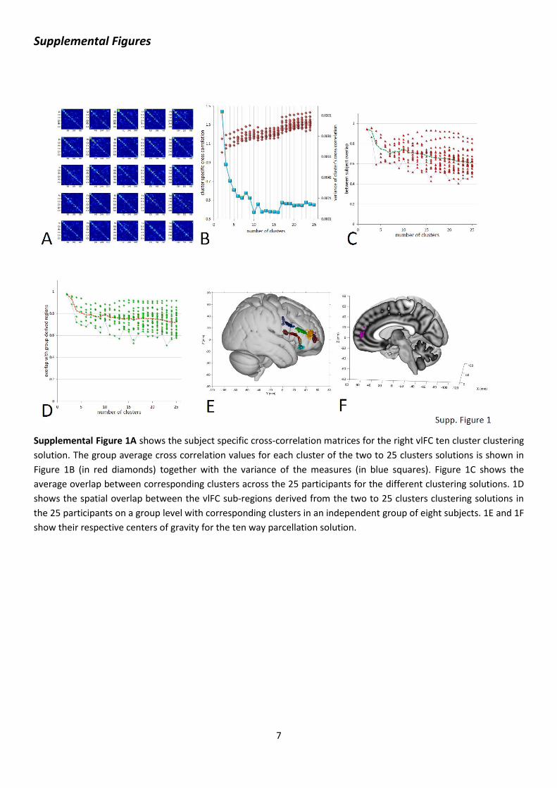
Supplemental Figure 1A shows the subject specific cross-correlation matrices for the right vlFC ten cluster clustering

solution. The group average cross correlation values for each cluster of the two to 25 clusters solutions is shown in

Figure 1B (in red diamonds) together with the variance of the measures (in blue squares). Figure 1C shows the

average overlap between corresponding clusters across the 25 participants for the different clustering solutions. 1D

shows the spatial overlap between the vlFC sub-regions derived from the two to 25 clusters clustering solutions in

the 25 participants on a group level with corresponding clusters in an independent group of eight subjects. 1E and 1F

show their respective centers of gravity for the ten way parcellation solution.

8

Supplemental Figure 2 shows the results of an iterative parcellation of vlFC similar to the one used by Beckmann and

colleagues (2009) in the anterior cingulate cortex. The parcellation started with the exact same vlFC ROI (red in

leftmost panel). The first parcellation (grey arrow with “1.”) divided the original vlFC ROI into an anterior (blue in

leftmost grey square) and a posterior (red) region. A multiple regression showed, that these two areas have

significantly different resting state coupling profiles with the rest of the brain (right part of leftmost grey square).

9

The group-parcels resulting from this first parcellation into two sub-regions were then used as an ROI for the next

parcellation attempt which again parcellated them further into two sub-regions (grey arrows with “2.”). In this way

the vlFC was parcellated into subregions with 3-4 parcellation steps. Parcellation was stopped if the respective parcel

/ ROI could not be sub-divided further reliably in all subjects.

Supplemental Figure 3 is the equivalent to figure 2 in the main text for the left vlFC: 2A shows the left vlFC ROI. 2B shows the result of the twelve cluster parcellation.

10

Supplemental Figure 4 shows on the left site of each panel the resting state fMRI based functional connectivity

patterns of each of the twelve left vlFC sub regions together with their respective spider plots. The right site of each

panel depicts the coupling pattern of each suggested homologuous area in the macaque left vlFC together with the

respective spider plot.

11

Supplemental Figure 5: Additional parcellation analyses were conducted in order to show that IFJ and IFS could

reliably be distinguished from 8Av and 9/46, respectively. An ROI comprising area IFJ as described here and 8A as

described by (Sallet et al., 2013) could be parcellated in all 25 subjects (top left). We established in a multiple

regression that these two areas have significantly different resting state coupling profiles with the rest of the brain

(top right). We also tested if it would be possible to reliably parcellate a ROI containing the 9/46v region described

by (Sallet et al., 2013) and the IFS area into two distinct regions (bottom left). We established, in a multiple

regression, that these two areas have significantly different resting state coupling profiles with the rest of the brain

(bottom right).

12

13

Supplemental Figure 6 shows the results of the between species matching of functional connectivity patterns. Each

human right vlFC sub-region was compared to all cytoarchitectonically defined macaque vlFC regions according to

their coupling patterns. For each human vlFC region we show a bar chart where the height of each bar represents

the distance between the connectivity fingerprints of the human vlFC region in question and each macaque vlFC

regions. The lowest bar indicates the macaque area that is least different (most similar) to the human vlFC area

investigated in terms of its coupling patterns with the rest of the brain. The distance between the functional coupling

scores of each human vlFC sub-region and 16 areas in macaque vlFC suggested that the human vlFC sub-regions

matched the macaque sub-regions as described in the main text and figures 4, 5, 6 and 8.

Supplemental Figure 7 shows the rank of four regions in the temporal lobe among the 19 regions used to generate

the spider plots in main text figures 4, 5, 6, and 8 for humans and macaques. High values mean that the coupling

strength (average z-value in the ROI of the parcel derived z-maps) between the respective vlFC region and the

temporal lobe region ranks very high among all target regions of interest (e.g., in the top left we can see that the IFJ

functional connectivity z-map shows very high coupling with planum temporale in the human [green boxplot], but

area 44 [the proposed macaque homologue of IFJ] shows relatively low coupling with area Tpt [the macaque

homologue of the planum temporale, red boxplot]; this difference is even significant when tested with a Mann–

Whitney–Wilcoxon rank-sum test with p < 0.05). “Cold colours” (green, cyan, green-yellow and olive) are used for

the human temporo-occipital ROIs and “warm colours” (red, pink, orange, lilac) for the macaque ROIs. The ROIs are

depicted on the human and macaque standard brain surface with the exact same colours as used in the boxplots.

14

Supplemental Figure 8 shows fMRI derived functional connectivity patterns of two auditory association areas in the

human and macaque (planum temporale and Tpt in blue and a voice-sensitive area in the anterior parabelt region in

the human and the macaque in orange) and the functional coupling with areas in the vlFC and cingulate cortex in the

15

left hemisphere. The two top graphs show the functional connectivity of planum temporale / Tpt (blue, left top

graph) and anterior parabelt region (orange, right top graph) with the anatomically defined vlFC subregions. The two

bottom graphs show the functional connectivity of planum temporale / Tpt (blue, left bottom graph) and anterior

parabelt region (orange, right bottom graph) with anatomically defined cingulate sub-regions. Graphs show the

ranking of functional connectivity of the auditory association areas with the vlFC and the cingulate ROIs in two

separate ranking analyses among all ROIs presented in the spider plots before (see figure 4-6 and 8). Asterisks mark

significant between species differences according to Mann–Whitney–Wilcoxon rank-sum test with p<0.05. The left

part of this figure is identical to Figure 7 in the main text.

16

17

Supplemental Figure 9 shows the same analysis as SFig 8 for the left hemisphere (planum temporale / Tpt, left TS2

and their interactions with left vlFC and left cingulate cortex).

Supplemental Figure 10 A shows a matrix of the spatial correlation between the sub-region specific resting state

functional connectivity patterns of areas IFJ, 44 and 45 (as shown in main text figures 5 and 6) and the ALE maps for

various different cognitive tasks and cognitive concepts established using the BrainMap database

(www.brainmap.org). See Supplemental table 4 for more information. B and C show cross correlation matrix of the

resting state BOLD time-courses in vlFC regions in human (B) and macaque (C). Human vlFC regions show

significantly stronger coupling between some prefrontal regions (black asterisks show significant difference in a

between species t-test on the Fisher-transformed correlation coefficient) but also weaker coupling between

premotor regions (indicated by white asterisks). D shows the parcellation derived sub-regions plotted on the MNI152

standard brain in a coronal (left), three sagittal (middle) and axial (right) slices.

18

Supplemental Tables

Area Abbreviation MNI coordinates (x, y, z)

Study

Ventro-Medial Prefrontal Cortex

VMPFC

8 44 -14

Cluster 2 in (Beckmann et al., 2009) and area 14m in (Mackey and Petrides, 2010); also cf (Boorman et al., 2011)

Area 32 32 8 42 0

(Vogt et al., 1995); also cf (Kolling et al., 2012)

Area 9 medial 9m 9 43 46

Cf cluster 3 in (Sallet et al., 2013) suggested to be area 9

Area 9/46 dorsal 9/46d 38 40 36

Cf. cluster 5 in (Sallet et al., 2013) suggested to be 9/46d

Area 8A / Frontal Eye Field

8A 32 12 56

Cf cluster 8 in (Sallet et al., 2013) and 8Ad in (Petrides, 2005) suggested to be 8A

Pre-Supplementary Motor Cortex

PreSMA 6 6 53

Cf. Pre-SMA in (Mayka et al., 2006)

Supplementary Motor Cortex

SMA 4 -8 54

Cf. SMA in (Mayka et al., 2006)

Premotor Cortex, dorsal part

PMd -30 -2 58

Cf. PMd in (Mayka et al., 2006)

Area PFop PFop 58 -16 28

Cf. PFop in (Caspers et al., 2013) and red cluster in (Mars et al., 2011) suggested to be PFop

Anterior Intraparietal Area

AIP 52 -32 44

Cf. blue IPL cluster in (Mars et al., 2011) suggested to be AIP

Ventral Intraparietal Area VIP 36 -42 50

Cf. red SPL cluster in (Mars et al., 2011) suggested to be VIP

Mid-Intraparietal Sulcus LIP 22 -64 52

Cf. magenta SPL cluster in (Mars et al., 2011) suggested to be LIP

Mid- Inferior Parietal Lobule

PFm 50 -44 40

Cf. green cluster in (Mars et al., 2011) suggested to be PFm

Area PG PG 38 -68 38

Yellow/orange cluster in (Mars et al., 2011) (suggested to be PGp)

Posterior Cingulate Cortex 23 10 -50 30

Cf (Beckmann et al., 2009) and (Vogt et al., 1995)

Fusiform Face Area FFA 42 -50 -18 Cf. (Higo et al., 2011)

Parahippocampal Place Area

PPA 28 -48 -16

Cf. (Higo et al., 2011)

Voice sensitive superior temporal Gyrus

voice 48 6 -12

Cf. (Belin et al., 2000)

Temporal Pole TP 34 12 -36

Interior temporopolar region (ITP) in (Mai et al., 2008)

Supplemental Table 1 : human brain areas investigated

19

Area Abbreviation used subsequently

MNI coordinates (x, y, z)

Ventro-Medial Prefrontal Cortex VMPFC 1.75 15.5 -1.75

Area 32 32 1.5 15.5 5.25

Area 9 medial 9m 1.5 19 12.5

Area 9/46 dorsal 946d 11.75 12.75 10.25

Area 8A / Frontal Eye Field 8A 13.5 8 13.25

Pre-Supplementary Motor Cortex preSMA 1.5 11.75 15.25

Supplementary Motor Cortex SMA 2.25 6.25 18

Premotor Cortex, dorsal part PMd 12.25 -0.25 17

Area PFop PFop 21.5 -8 6

Anterior Intraparietal Area AIP 18.25 -8 11.75

Ventral Intraparietal Area VIP 11 -14.75 12.75

Mid-Intraparietal Sulcus LIP 10.5 -19 17

Mid- Inferior Parietal Lobule pf 21 -11.75 13.75

Area PG pg 16.5 -15.25 16.25

Posterior Cingulate Cortex 23 1.25 -16 8.75

Fusiform Face Area Face sensitive STS 23.5 -10 -4

Parahippocampal Place Area Place sensitive ITG 20 -2 -11

Voice sensitive superior temporal Gyrus Ts2 22 0 -2.5

Temporal Pole TP 18.75 7 -7.25

Area F5p F5p 15.25 4 10.75

Area F5c F5c 20.75 4 7

Area F5a F5a 19 6.75 6.5

Area ProM ProM 20 8 -2.75

Area Area 8Av 8Av 16.5 8.5 10.25

Area 44 44 15.25 8.75 3

Area 45B 45B 16.5 10 8

Area 45A 45A 16.75 13.25 4.25

Area 47 47 12.5 19.75 6

Area 9/46v 9/46v 13.75 14.25 8

Area 46 46 11 13.5 7.5

Anterior Insula AI 15.25 6.25 -4

Area 10d 10d 5.75 22.25 9.5

Area 10v 10v 5 24.25 3.5

Area 10m 10m 1.25 25 5

Supplemental Table 2 macaque brain areas investigated

20

Area in Human Human Area Abbreviation

Monkey Area Abbreviation

Area in Rhesus Monkey

Study / Atlas

Ventro-Medial Prefrontal Cortex

VMPFC VMPFC

Area 14 (Mackey and Petrides, 2010; Saleem and Logothetis, 2007)

Area 32 32 32 Area 32 (Beckmann et al., 2009; Mackey and Petrides, 2010; Ongur et al., 2003; Saleem and Logothetis, 2007)

Area 9 medial 9m 9m Area 9m (McLaren et al., 2009; Sallet et al., 2013)

Area 9/46 dorsal 946d 946d Area 9/46D (Paxinos et al., 2000; Sallet et al., 2013)

Area 8A / Frontal Eye Field

8A 8A Area 8A (Saleem and Logothetis, 2007; Sallet et al., 2013)

Pre-Supplemental Motor Cortex

PreSMA preSMA Agranular F6 (Saleem and Logothetis, 2007; Sallet et al., 2013)

Supplemental Motor Cortex

SMA SMA Agranular Frontal Area F3

(Saleem and Logothetis, 2007; Sallet et al., 2013)

Premotor Cortex, dorsal part

PMd PMd Area F2 6DR 6DC

(Saleem and Logothetis, 2007; Sallet et al., 2013)

Area PFop PFop PFop Area PFop (Mars et al., 2011; Paxinos et al., 2000)

Ventral Intraparietal Area

AIP AIP Area AIP (Mars et al., 2011; Paxinos et al., 2000)

Mid-Intraparietal Sulcus

VIP VIP Area VIP (Mars et al., 2011; Paxinos et al., 2000)

Lateral Intraparietal Sulcus

LIP LIP Area LIP (Mars et al., 2011; Paxinos et al., 2000)

Mid- Inferior Parietal Lobule

PFm Pf Area PF (Mars et al., 2011; Paxinos et al.,

2000)

Area PG PG Pg Area PG (Mars et al., 2011; Paxinos et al., 2000)

Posterior Cingulate Cortex

23 23 Area 23 (Paxinos et al., 2000) (Beckmann et al., 2009; Vogt et al., 1992)

Fusiform Face Area FFA Face sensitive STS

Face sensitive superior temporal sulcus

(Bell et al., 2011)

Parahippocampal Place Area

PPA Place sensitive ITG

Place sensitive inferior temporal gyrus

(Bell et al., 2011)

Voice sensitive superior temporal Gyrus

voice Ts2 Voice sensitive TS2 (Petkov et al., 2008)

Temporal Pole TP TP dorsal temporal pole

(Saleem and Logothetis, 2007)

Supplemental Table 3: correspondences between human and macaque areas outside of vlFC

21

Table 4: meta-analysis of activation patterns in cognitive tasks

Search Criteria papers participants experiments locations

Experiments: Paradigm Class: Go/No-Go AND Activations only 86 2076 301 2743 Experiments: Paradigm Class: Task Switching AND Activations only 42 831 151 1282

Experiments: Paradigm Class: n-back AND Activations only 120 2950 481 3682 Experiments: Paradigm Class: Face Monitor / Discrimination AND Activations only 144 2985 645 4312 Experiments: Behavioral Domain: Cognition: Language - Semantics AND Activations only 253 3990 945 7245 Experiments: Paradigm Class: Paired Associate Recall AND Activations only 43 808 161 1184

22

Supplemental References

Aron, A.R., and Poldrack, R.A. (2006). Cortical and subcortical contributions to Stop signal response inhibition: role of the subthalamic nucleus. J Neurosci 26, 2424-2433. Beckmann, M., Johansen-Berg, H., and Rushworth, M.F. (2009). Connectivity-based parcellation of human cingulate cortex and its relation to functional specialization. J Neurosci 29, 1175-1190. Belin, P., Zatorre, R.J., Lafaille, P., Ahad, P., and Pike, B. (2000). Voice-selective areas in human auditory cortex. Nature 403, 309-312. Bell, A.H., Malecek, N.J., Morin, E.L., Hadj-Bouziane, F., Tootell, R.B., and Ungerleider, L.G. (2011). Relationship between functional magnetic resonance imaging-identified regions and neuronal category selectivity. J Neurosci 31, 12229-12240. Boorman, E.D., Behrens, T.E., and Rushworth, M.F. (2011). Counterfactual choice and learning in a neural network centered on human lateral frontopolar cortex. PLoS Biol 9, e1001093. Caspers, S., Schleicher, A., Bacha-Trams, M., Palomero-Gallagher, N., Amunts, K., and Zilles, K. (2013). Organization of the human inferior parietal lobule based on receptor architectonics. Cereb Cortex 23, 615-628. Chikazoe, J., Jimura, K., Asari, T., Yamashita, K., Morimoto, H., Hirose, S., Miyashita, Y., and Konishi, S. (2009a). Functional dissociation in right inferior frontal cortex during performance of go/no-go task. Cereb Cortex 19, 146-152. Chikazoe, J., Jimura, K., Hirose, S., Yamashita, K., Miyashita, Y., and Konishi, S. (2009b). Preparation to inhibit a response complements response inhibition during performance of a stop-signal task. J Neurosci 29, 15870-15877. Corbetta, M., Patel, G., and Shulman, G.L. (2008). The reorienting system of the human brain: from environment to theory of mind. Neuron 58, 306-324. Derrfuss, J., Brass, M., Neumann, J., and von Cramon, D.Y. (2005). Involvement of the inferior frontal junction in cognitive control: meta-analyses of switching and Stroop studies. Hum Brain Mapp 25, 22-34. Dosenbach, N.U., Visscher, K.M., Palmer, E.D., Miezin, F.M., Wenger, K.K., Kang, H.C., Burgund, E.D., Grimes, A.L., Schlaggar, B.L., and Petersen, S.E. (2006). A core system for the implementation of task sets. Neuron 50, 799-812. Eickhoff, S.B., Laird, A.R., Grefkes, C., Wang, L.E., Zilles, K., and Fox, P.T. (2009). Coordinate-based activation likelihood estimation meta-analysis of neuroimaging data: a random-effects approach based on empirical estimates of spatial uncertainty. Hum Brain Mapp 30, 2907-2926. Fedorenko, E., Behr, M.K., and Kanwisher, N. (2011). Functional specificity for high-level linguistic processing in the human brain. Proc Natl Acad Sci U S A 108, 16428-16433. Fedorenko, E., Duncan, J., and Kanwisher, N. (2012). Language-Selective and Domain-General Regions Lie Side by Side within Broca's Area. Curr Biol 22, 2059-2062. Friederici, A.D. (2006). Broca's area and the ventral premotor cortex in language: functional differentiation and specificity. Cortex 42, 472-475. Friederici, A.D., Bahlmann, J., Heim, S., Schubotz, R.I., and Anwander, A. (2006). The brain differentiates human and non-human grammars: functional localization and structural connectivity. Proc Natl Acad Sci U S A 103, 2458-2463. Higo, T., Mars, R.B., Boorman, E.D., Buch, E.R., and Rushworth, M.F. (2011). Distributed and causal influence of frontal operculum in task control. Proc Natl Acad Sci U S A 108, 4230-4235. Hirose, S., Chikazoe, J., Jimura, K., Yamashita, K., Miyashita, Y., and Konishi, S. (2009). Sub-centimeter scale functional organization in human inferior frontal gyrus. Neuroimage 47, 442-450. Johansen-Berg, H., Behrens, T.E., Robson, M.D., Drobnjak, I., Rushworth, M.F., Brady, J.M., Smith, S.M., Higham, D.J., and Matthews, P.M. (2004). Changes in connectivity profiles define functionally distinct regions in human medial frontal cortex. Proc Natl Acad Sci U S A 101, 13335-13340. Kolling, N., Behrens, T.E., Mars, R.B., and Rushworth, M.F. (2012). Neural mechanisms of foraging. Science 336, 95-98. Laird, A.R., Lancaster, J.L., and Fox, P.T. (2005). BrainMap: the social evolution of a human brain mapping database. Neuroinformatics 3, 65-78. Laird, A.R., Lancaster, J.L., and Fox, P.T. (2009). Lost in localization? The focus is meta-analysis. Neuroimage 48, 18-20. Mackey, S., and Petrides, M. (2010). Quantitative demonstration of comparable architectonic areas within the ventromedial and lateral orbital frontal cortex in the human and the macaque monkey brains. Eur J Neurosci 32, 1940-1950. Mai, J.r.K., Voss, T., and Paxinos, G. (2008). Atlas of the human brain, 3rd edn (London: Elsevier/Academic Press).

23

Mars, R.B., Jbabdi, S., Sallet, J., O'Reilly, J.X., Croxson, P.L., Olivier, E., Noonan, M.P., Bergmann, C., Mitchell, A.S., Baxter, M.G., et al. (2011). Diffusion-weighted imaging tractography-based parcellation of the human parietal cortex and comparison with human and macaque resting-state functional connectivity. J Neurosci 31, 4087-4100. Mayka, M.A., Corcos, D.M., Leurgans, S.E., and Vaillancourt, D.E. (2006). Three-dimensional locations and boundaries of motor and premotor cortices as defined by functional brain imaging: a meta-analysis. Neuroimage 31, 1453-1474. McLaren, D.G., Kosmatka, K.J., Oakes, T.R., Kroenke, C.D., Kohama, S.G., Matochik, J.A., Ingram, D.K., and Johnson, S.C. (2009). A population-average MRI-based atlas collection of the rhesus macaque. Neuroimage 45, 52-59. Ongur, D., Ferry, A.T., and Price, J.L. (2003). Architectonic subdivision of the human orbital and medial prefrontal cortex. The Journal of comparative neurology 460, 425-449. Paxinos, G., Huang, X.F., and Toga, A.W. (2000). The rhesus monkey brain in stereotaxic coordinates (San Diego ; London: Academic). Petkov, C.I., Kayser, C., Steudel, T., Whittingstall, K., Augath, M., and Logothetis, N.K. (2008). A voice region in the monkey brain. Nat Neurosci 11, 367-374. Petrides, M. (2005). Lateral prefrontal cortex: architectonic and functional organization. Philos Trans R Soc Lond B Biol Sci 360, 781-795. Saleem, K.S., and Logothetis, N.K. (2007). A combined MRI and histology atlas of the rhesus monkey brain in stereotaxic coordinates (London ; Burlington, MA: Academic). Sallet, J., Mars, R.B., Noonan, M.P., Neubert, F.X., Jbabdi, S., O'Reilly, J.X., Filippini, N., Thomas, A.G., and Rushworth, M.F. (2013). The organization of dorsal frontal cortex in humans and macaques. J Neurosci 33, 12255-12274. Smith, S.M., Fox, P.T., Miller, K.L., Glahn, D.C., Fox, P.M., Mackay, C.E., Filippini, N., Watkins, K.E., Toro, R., Laird, A.R., and Beckmann, C.F. (2009). Correspondence of the brain's functional architecture during activation and rest. Proc Natl Acad Sci U S A 106, 13040-13045. Verbruggen, F., Aron, A.R., Stevens, M.A., and Chambers, C.D. (2010). Theta burst stimulation dissociates attention and action updating in human inferior frontal cortex. Proc Natl Acad Sci U S A 107, 13966-13971. Vincent, J.L., Patel, G.H., Fox, M.D., Snyder, A.Z., Baker, J.T., Van Essen, D.C., Zempel, J.M., Snyder, L.H., Corbetta, M., and Raichle, M.E. (2007). Intrinsic functional architecture in the anaesthetized monkey brain. Nature 447, 83-86. Vogt, B.A., Finch, D.M., and Olson, C.R. (1992). Functional heterogeneity in cingulate cortex: the anterior executive and posterior evaluative regions. Cereb Cortex 2, 435-443. Vogt, B.A., Nimchinsky, E.A., Vogt, L.J., and Hof, P.R. (1995). Human cingulate cortex: surface features, flat maps, and cytoarchitecture. The Journal of comparative neurology 359, 490-506. Vossel, S., Weidner, R., and Fink, G.R. (2011). Dynamic coding of events within the inferior frontal gyrus in a probabilistic selective attention task. J Cogn Neurosci 23, 414-424.