Optimization Theory and

Applications

SupplementalLectureforMathematicalBackground

Prof. Chun-Hung Liu

2016/10/18 Lecture:Supplement 1

Dept. of Electrical and Computer EngineeringNational Chiao Tung University

Fall 2016

2016/10/18 Lecture:Supplement 2

Function Notation• When we write

we mean that f is a function on the set mapping into the set B. Thus the notation means that f maps (some) n-vectors into m-vectors.

domf ✓ Af : Rn ! Rm

• As an example consider the function given byf : Sn ! R

with . The notation specifies the syntax of f: it takes as argument a symmetric matrix, and returns a real number. The notation specifies which symmetric matrices are valid input arguments for f (i.e., only positive definite ones).

domf = S

n++ f : Sn ! R

n⇥ nn⇥ n

domf = S

n++

2016/10/18 Lecture:Supplement 3

Gradient, Jacobian, Hessian

• A gradient is the derivative of a scalar with respect to a vector.

rx

f(x) =

f(x) = 2x1x2 + x

22 + x1x

23• Example: if then its gradient is

rx

f(x) =

2016/10/18 Lecture:Supplement 4

• A Jacobian is a the derivative of a vector with respect to a transposed vector.

Gradient, Jacobian, Hessian

• Example: If we have the function

then its Jacobian is

, f(x) = [f1(x), f2(x), . . . , fk(x)]

2016/10/18 Lecture:Supplement 5

Gradient, Jacobian, Hessian

• The Hessian is derivative of a Gradient with respect to a transposed vector.

r2x

f(x) =

Recall that our above Gradient is

The Hessian is

2016/10/18 Lecture:Supplement 6

Trace Derivative of Matrix• If and , then X 2 Rn⇥m f(Y) = tr(Y)

@f(Y)

@X=

where is what we put in the ijth place in our derivative matrix.@tr(Y)

@xij

Thus,

because is what we put in the jith place in our derivative matrix.

@tr(Y)

@xji

2016/10/19 Lecture:Supplement 7

Product Rule for Vector and Matrix

• Suppose u(x) and v(x) are scalar functions of x. Recall from your Calculus class, you must see the following product rule:

• Now, we want to translate this to matrices and traces of matrices:

• If we take the derivative of the matrix product with respect to a scalar:

2016/10/19 Lecture:Supplement 8

Then we find that the i,jth place in our new derivative matrix is

Product Rule for Vector and Matrix

• Since the picked elements is arbitrary, we can generalize:

2016/10/19 Lecture:Supplement 9

Chain Rule for Vector and Matrix• Let us first see an example. Suppose

Now if

2016/10/19 Lecture:Supplement 10

Chain Rule for Vector and MatrixBut, we know

So, another way of getting the same result:

• In other words, if then f : Rn ! R

df(x) =nX

i=1

@f(x)

@xi· @xi

@t

dt = rf(x)T@x

@t

dt

2016/10/19 Lecture:Supplement 11

Directional Derivative of Vectors

• The standard derivative definition:

• In vector calculus, we have the directional derivative defined as

• Now, our function is a surface (a scalar function of as many dimensional inputs as there are elements in x), so the derivative will change at a multidimensional point x based on the direction we travel from that point.

• Think of what happens if you were to stand on a mountain and turn around in a circle: in some directions, the slope will be very steep (and you might fall off the mountain), but in other directions, there will barely be any slope at all.

2016/10/19 Lecture:Supplement 12

Directional Derivative of Vectors • Actually, we can write

Dw

f(x) = w

T @f(x)

@x= w

Trx

f(x)

• Example: Let . Find f(x) = x

TQx r

x

f(x) =?

= w

TQx+ x

TQw + limt!0

twTQw

Dwf(x) = limt!0

f(x+ tw)

t= lim

t!0

(x+ tw)TQ(x+ tw)� x

TQx

t

= 2wTQx

rx

f(x) = Qx

r2x

f(x) = Q

2016/10/19 Lecture:Supplement 13

Table of Gradients • For , and , we have the following x 2 Rn A 2 Rm⇥n b 2 Rm

2016/10/19 Lecture:Supplement 14

Table of Gradients • For , we have the following x, a, b 2 Rn

2016/10/19 Lecture:Supplement 15

• Now we can extend our directional derivative definition to matrices

where Y is a matrix with the same dimension as X.

• Similarly, we have

(We ca use this definition to find )

tr

✓YT @f(X)

@X

◆

@f(X)

@X

Directional Derivative of Matrices

2016/10/19 Lecture:Supplement 16

Directional Derivative of Matrices • Example: Suppose and we want to find

= ?

By definition, we know

2016/10/19 Lecture:Supplement 17

Directional Derivative of Matrices • So we can have

= tr(Y TAT ) = tr

✓Y T @f(X)

@X

◆

= AT

• Example: Let . Find @f(X)

@X=?

2016/10/19 Lecture:Supplement 18

Directional Derivative of Matrices

(Because )tr(UV ) = tr(V U)

2016/10/19 Lecture:Supplement 19

Directional Derivative of Matrices

2016/10/19 Lecture:Supplement 20

Directional Derivative of Vectors

• Example: Consider the function and . f(X) = log det(X)

f : Sn++ ! R

• One (tedious) way to find the gradient of f is to follow the direction derivative introduced in above. Instead, we will directly find the first-order approximation of f at .

• Let be close to X, and let (which is assumed to be small). Thus we have

Now we would like to show .

X 2 Sn++

Z 2 Sn++ �X = Z �X

where is the ith eigenvalue of�i X�1/2�XX�1/2

rf(X) = X�1

2016/10/19 Lecture:Supplement 21

Directional Derivative of Vectors • Now we use the fact that is small, which implies are small, so to

first order we have . Using this first-order approximation in the expression above, we get

�X �i

log(1 + �i) ⇡ �i

Thus, the first-order approximation of f at X is the affine function of Zgiven by

Noting that the second term on the right hand side is the standard inner product of and Z-X . So we can identify as the gradient of f at X.X�1 X�1

2016/10/19 Lecture:Supplement 22

Table of Gradients

2016/10/19 Lecture:Supplement 23

Table of Gradients

2016/10/18 Lecture:Supplement 24

Symmetric Eigenvalue Decomposition

• Suppose , i.e., A is a real symmetric matrix. Then A can be factored as

A 2 Sn n⇥ n

where is an orthogonal matrix (or called unitary matrix), i.e., satisfies , and . The (real) numbers are the eigenvalues of A, The columns of Q form an orthonormal set ofeigenvectors of A.

QTQ = I ⇤ = diag(�1, . . . ,�n) �i

• The determinant and trace can be expressed in terms of the eigenvalues,

as can the spectral and Frobenius norms,

2016/10/18 Lecture:Supplement 25

Definiteness and Matrix Inequalities• The largest and smallest eigenvalues satisfy

In particular, for any x, we have

• A matrix is called positive definite if for all , . We denote this as . By the inequality above, we see that if and only all its eigenvalues are positive, i.e., . We use to denote the set of positive definite matrices in .

A 2 Snx 6= 0

x

TAx > 0

A � 0 A � 0�min(A) > 0 Sn

++

Sn

• For , we use to mean , and so on.A,B 2 Sn A � B B �A � 0

2016/10/18 Lecture:Supplement 26

Singular Value Decomposition (SVD)• Symmetric squareroot: Let , with eigenvalue decomposition

. We define the (symmetric) squareroot of A as

A 2 Sn+

The squareroot is the unique symmetric positive semidefinite solution of the equation .

A1/2

X2 = A

• Suppose with . Then A can be factored asA 2 Rm⇥n rankA = r

(SVD)

2016/10/18 Lecture:Supplement 27

Definiteness and Matrix Inequalities• The columns of U are called left singular vectors of A, the columns

of V are right singular vectors, and the numbers are the singular values. The singular value decomposition can be written

�i

where are the left singular vectors, and are the right singular vectors.

ui 2 Rm vi 2 Rn

• The singular value decomposition of a matrix A is closely related to the eigenvalue decomposition of the (symmetric, nonnegative definite) matrix . So we can writeATA

So we conclude that its nonzero eigenvalues are the singular values of Asquared, and the associated eigenvectors of are the right singular vectors of A.

ATA

2016/10/18 Lecture:Supplement 28

Pseudo-inverse of Matrices• Let be the singular value decomposition of

with with rank A=r. We define the pseudo-inverse or Moore-Penrose inverse of A as

A = U⌃V T A 2 Rm⇥n

• If , then . If , then. If A is square and nonsingular, then .

rankA = n A† = (ATA)�1AT rankA = mA† = AT (AAT )�1 A† = A�1

• The pseudo-inverse comes up in problems involving least-squares, minimum norm, quadratic minimization, and (Euclidean) projection. For example, is a solution of the least-squares problemA†b

When the solution is not unique, gives the solution with minimum(Euclidean) norm.

A†b

2016/10/18 Lecture:Supplement 29

Schur Complement• Consider a matrix partitioned asX 2 Sn

where . If , the matrixA 2 Sn det(A) 6= 0

is called the Schur complement of A in X. Schur complements arise in several contexts, and appear in many important formulas and theorems. For example, we have

2016/10/19 Lecture:Supplement 30

• The Schur complement comes up in solving linear equations, by eliminating one block of variables. For example,

Schur Complement

assuming . Eliminating x from the top block equation and substituting it into the bottom block equation yield

det(A) 6= 0

v = BTA�1u+ Sy y = S�1(v �BTA�1u)

Substituting this into the first equation yields

2016/10/19 Lecture:Supplement 31

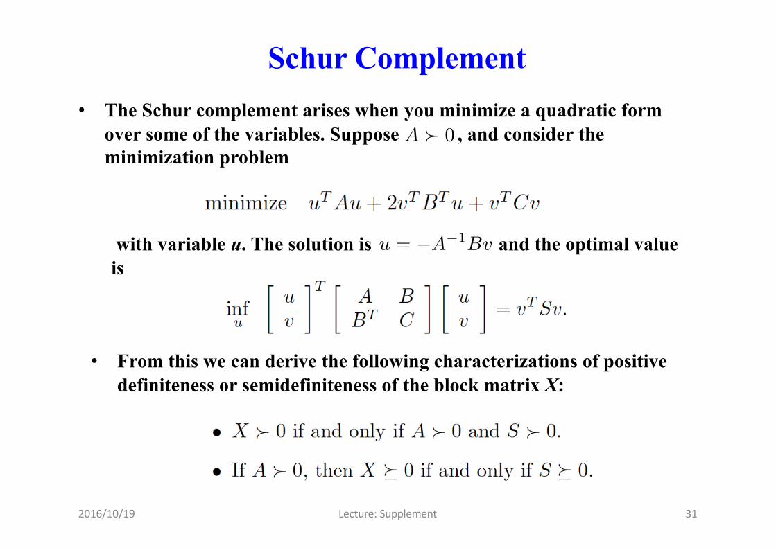
Schur Complement• The Schur complement arises when you minimize a quadratic form

over some of the variables. Suppose , and consider the minimization problem

A � 0

with variable u. The solution is and the optimal value is

u = �A�1Bv

• From this we can derive the following characterizations of positive definiteness or semidefiniteness of the block matrix X: