Supplemental Material

Title

Measuring the Contribution of Agricultural Conservation Practices to Observed Trends and

Recent Condition in Water Quality Indicators in Ohio, USA

Author

Robert J. Miltner

Ohio Environmental Protection Agency, 4675 Homer-Ohio Lane, Groveport, Ohio 43125.

Robert.miltner@epa.ohio.gov

(614) 836-8796

12 Pages

3 Tables

6 Figures

S1

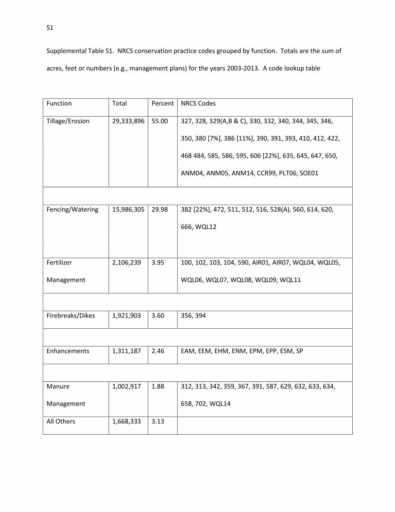
Supplemental Table S1. NRCS conservation practice codes grouped by function. Totals are the sum of

acres, feet or numbers (e.g., management plans) for the years 2003-2013. A code lookup table

Function Total Percent NRCS Codes

Tillage/Erosion

29,333,896 55.00 327, 328, 329(A,B & C), 330, 332, 340, 344, 345, 346,

350, 380 [7%], 386 [11%], 390, 391, 393, 410, 412, 422,

468 484, 585, 586, 595, 606 [22%], 635, 645, 647, 650,

ANM04, ANM05, ANM14, CCR99, PLT06, SOE01

Fencing/Watering 15,986,305 29.98 382 [22%], 472, 511, 512, 516, 528(A), 560, 614, 620,

666, WQL12

Fertilizer

Management

2,106,239 3.95 100, 102, 103, 104, 590, AIR01, AIR07, WQL04, WQL05,

WQL06, WQL07, WQL08, WQL09, WQL11

Firebreaks/Dikes 1,921,903 3.60 356, 394

Enhancements 1,311,187 2.46 EAM, EEM, EHM, ENM, EPM, EPP, ESM, SP

Manure

Management

1,002,917 1.88 312, 313, 342, 359, 367, 391, 587, 629, 632, 633, 634,

658, 702, WQL14

All Others 1,668,333 3.13

S2

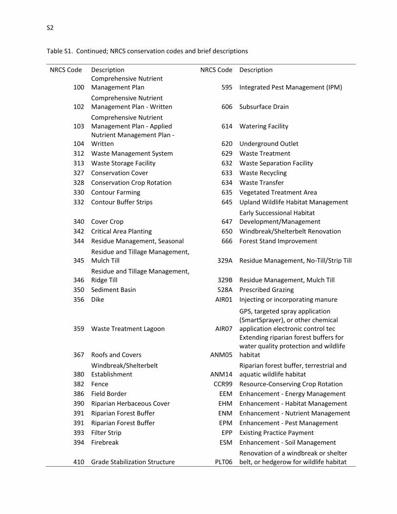
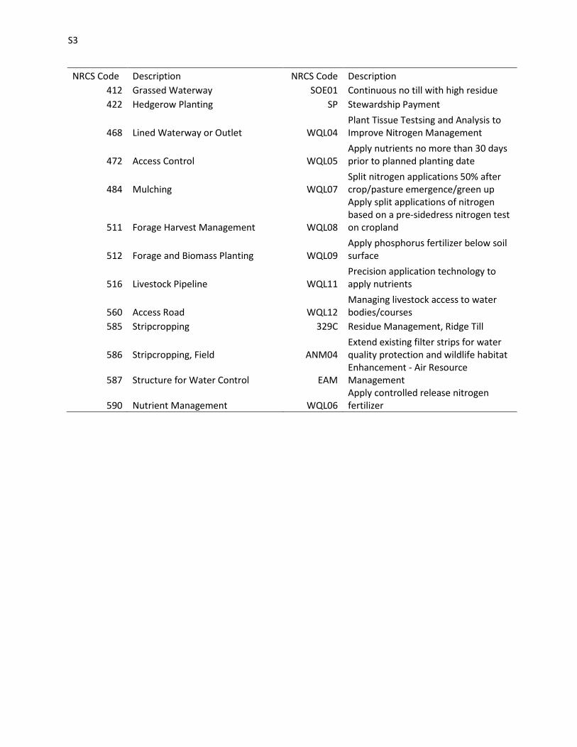
Table S1. Continued; NRCS conservation codes and brief descriptions

NRCS Code Description NRCS Code Description

100 Comprehensive Nutrient Management Plan 595 Integrated Pest Management (IPM)

102 Comprehensive Nutrient Management Plan - Written 606 Subsurface Drain

103 Comprehensive Nutrient Management Plan - Applied 614 Watering Facility

104 Nutrient Management Plan - Written 620 Underground Outlet

312 Waste Management System 629 Waste Treatment 313 Waste Storage Facility 632 Waste Separation Facility 327 Conservation Cover 633 Waste Recycling 328 Conservation Crop Rotation 634 Waste Transfer 330 Contour Farming 635 Vegetated Treatment Area 332 Contour Buffer Strips 645 Upland Wildlife Habitat Management

340 Cover Crop 647 Early Successional Habitat Development/Management

342 Critical Area Planting 650 Windbreak/Shelterbelt Renovation 344 Residue Management, Seasonal 666 Forest Stand Improvement

345 Residue and Tillage Management, Mulch Till 329A Residue Management, No-Till/Strip Till

346 Residue and Tillage Management, Ridge Till 329B Residue Management, Mulch Till

350 Sediment Basin 528A Prescribed Grazing 356 Dike AIR01 Injecting or incorporating manure

359 Waste Treatment Lagoon AIR07

GPS, targeted spray application (SmartSprayer), or other chemical application electronic control tec

367 Roofs and Covers ANM05

Extending riparian forest buffers for water quality protection and wildlife habitat

380 Windbreak/Shelterbelt Establishment ANM14

Riparian forest buffer, terrestrial and aquatic wildlife habitat

382 Fence CCR99 Resource-Conserving Crop Rotation 386 Field Border EEM Enhancement - Energy Management 390 Riparian Herbaceous Cover EHM Enhancement - Habitat Management 391 Riparian Forest Buffer ENM Enhancement - Nutrient Management 391 Riparian Forest Buffer EPM Enhancement - Pest Management 393 Filter Strip EPP Existing Practice Payment 394 Firebreak ESM Enhancement - Soil Management

410 Grade Stabilization Structure PLT06 Renovation of a windbreak or shelter belt, or hedgerow for wildlife habitat

S3

NRCS Code Description NRCS Code Description 412 Grassed Waterway SOE01 Continuous no till with high residue 422 Hedgerow Planting SP Stewardship Payment

468 Lined Waterway or Outlet WQL04 Plant Tissue Testsing and Analysis to Improve Nitrogen Management

472 Access Control WQL05 Apply nutrients no more than 30 days prior to planned planting date

484 Mulching WQL07 Split nitrogen applications 50% after crop/pasture emergence/green up

511 Forage Harvest Management WQL08

Apply split applications of nitrogen based on a pre-sidedress nitrogen test on cropland

512 Forage and Biomass Planting WQL09 Apply phosphorus fertilizer below soil surface

516 Livestock Pipeline WQL11 Precision application technology to apply nutrients

560 Access Road WQL12 Managing livestock access to water bodies/courses

585 Stripcropping 329C Residue Management, Ridge Till

586 Stripcropping, Field ANM04 Extend existing filter strips for water quality protection and wildlife habitat

587 Structure for Water Control EAM Enhancement - Air Resource Management

590 Nutrient Management WQL06 Apply controlled release nitrogen fertilizer

S4

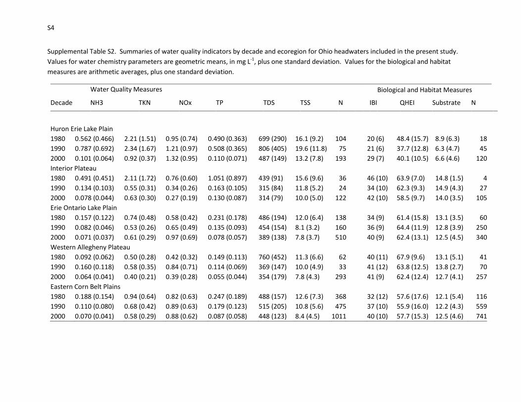
Supplemental Table S2. Summaries of water quality indicators by decade and ecoregion for Ohio headwaters included in the present study. Values for water chemistry parameters are geometric means, in mg L-1, plus one standard deviation. Values for the biological and habitat measures are arithmetic averages, plus one standard deviation.

Water Quality Measures

Biological and Habitat Measures

Decade NH3 TKN NOx TP TDS TSS N IBI QHEI Substrate N

Huron Erie Lake Plain 1980 0.562 (0.466) 2.21 (1.51) 0.95 (0.74) 0.490 (0.363) 699 (290) 16.1 (9.2) 104 20 (6) 48.4 (15.7) 8.9 (6.3) 18

1990 0.787 (0.692) 2.34 (1.67) 1.21 (0.97) 0.508 (0.365) 806 (405) 19.6 (11.8) 75 21 (6) 37.7 (12.8) 6.3 (4.7) 45 2000 0.101 (0.064) 0.92 (0.37) 1.32 (0.95) 0.110 (0.071) 487 (149) 13.2 (7.8) 193 29 (7) 40.1 (10.5) 6.6 (4.6) 120 Interior Plateau

1980 0.491 (0.451) 2.11 (1.72) 0.76 (0.60) 1.051 (0.897) 439 (91) 15.6 (9.6) 36 46 (10) 63.9 (7.0) 14.8 (1.5) 4 1990 0.134 (0.103) 0.55 (0.31) 0.34 (0.26) 0.163 (0.105) 315 (84) 11.8 (5.2) 24 34 (10) 62.3 (9.3) 14.9 (4.3) 27 2000 0.078 (0.044) 0.63 (0.30) 0.27 (0.19) 0.130 (0.087) 314 (79) 10.0 (5.0) 122 42 (10) 58.5 (9.7) 14.0 (3.5) 105 Erie Ontario Lake Plain

1980 0.157 (0.122) 0.74 (0.48) 0.58 (0.42) 0.231 (0.178) 486 (194) 12.0 (6.4) 138 34 (9) 61.4 (15.8) 13.1 (3.5) 60 1990 0.082 (0.046) 0.53 (0.26) 0.65 (0.49) 0.135 (0.093) 454 (154) 8.1 (3.2) 160 36 (9) 64.4 (11.9) 12.8 (3.9) 250 2000 0.071 (0.037) 0.61 (0.29) 0.97 (0.69) 0.078 (0.057) 389 (138) 7.8 (3.7) 510 40 (9) 62.4 (13.1) 12.5 (4.5) 340 Western Allegheny Plateau

1980 0.092 (0.062) 0.50 (0.28) 0.42 (0.32) 0.149 (0.113) 760 (452) 11.3 (6.6) 62 40 (11) 67.9 (9.6) 13.1 (5.1) 41 1990 0.160 (0.118) 0.58 (0.35) 0.84 (0.71) 0.114 (0.069) 369 (147) 10.0 (4.9) 33 41 (12) 63.8 (12.5) 13.8 (2.7) 70 2000 0.064 (0.041) 0.40 (0.21) 0.39 (0.28) 0.055 (0.044) 354 (179) 7.8 (4.3) 293 41 (9) 62.4 (12.4) 12.7 (4.1) 257 Eastern Corn Belt Plains

1980 0.188 (0.154) 0.94 (0.64) 0.82 (0.63) 0.247 (0.189) 488 (157) 12.6 (7.3) 368 32 (12) 57.6 (17.6) 12.1 (5.4) 116 1990 0.110 (0.080) 0.68 (0.42) 0.89 (0.63) 0.179 (0.123) 515 (205) 10.8 (5.6) 475 37 (10) 55.9 (16.0) 12.2 (4.3) 559 2000 0.070 (0.041) 0.58 (0.29) 0.88 (0.62) 0.087 (0.058) 448 (123) 8.4 (4.5) 1011 40 (10) 57.7 (15.3) 12.5 (4.6) 741

S5

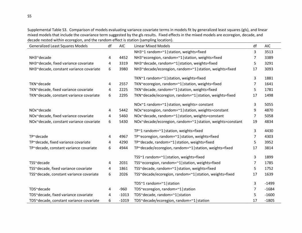
Supplemental Table S3. Comparison of models evaluating variance covariate terms in models fit by generalized least squares (gls), and linear mixed models that include the covariance term suggested by the gls results. Fixed effects in the mixed models are ecoregion, decade, and decade nested within ecoregion, and the random effect is station (sampling location). Generalized Least Squares Models df AIC Linear Mixed Models df AIC NH3~1 random=~1|station, weights=fixed 3 3513 NH3~decade 4 4452 NH3~ecoregion, random=~1|station, weights=fixed 7 3389 NH3~decade, fixed variance covariate 4 3319 NH3~decade, random=~1|station, weights=fixed 5 3291 NH3~decade, constant variance covariate 6 3980 NH3~decade/ecoregion, random=~1|station, weights=fixed 17 3093

TKN~1 random=~1|station, weights=fixed 3 1881 TKN~decade 4 2557 TKN~ecoregion, random=~1|station, weights=fixed 7 1641 TKN~decade, fixed variance covariate 4 2225 TKN~decade, random=~1|station, weights=fixed 5 1781 TKN~decade, constant variance covariate 6 2295 TKN~decade/ecoregion, random=~1|station, weights=fixed 17 1498

NOx~1 random=~1|station, weights= constant 3 5055 NOx~decade 4 5442 NOx~ecoregion, random=~1|station, weights=constant 9 4870 NOx~decade, fixed variance covariate 4 5460 NOx~decade, random=~1|station, weights=constant 7 5058 NOx~decade, constant variance covariate 6 5430 NOx~decade/ecoregion, random=~1|station, weights=constant 19 4834

TP~1 random=~1|station, weights=fixed 3 4430 TP~decade 4 4967 TP~ecoregion, random=~1|station, weights=fixed 7 4303 TP~decade, fixed variance covariate 4 4290 TP~decade, random=~1|station, weights=fixed 5 3952 TP~decade, constant variance covariate 6 4944 TP~decade/ecoregion, random=~1|station, weights=fixed 17 3814

TSS~1 random=~1|station, weights=fixed 3 1899 TSS~decade 4 2031 TSS~ecoregion, random=~1|station, weights=fixed 7 1785 TSS~decade, fixed variance covariate 4 1861 TSS~decade, random=~1|station, weights=fixed 5 1752 TSS~decade, constant variance covariate 6 2026 TSS~decade/ecoregion, random=~1|station, weights=fixed 17 1639

TDS~1 random=~1|station 3 -1499 TDS~decade 4 -960 TDS~ecoregion, random=~1|station 7 -1684 TDS~decade, fixed variance covariate 4 -1013 TDS~decade, random=~1|station 5 -1600 TDS~decade, constant variance covariate 6 -1019 TDS~decade/ecoregion, random=~1|station 17 -1805

S6

Supplemental Table S3. Continued - comparison of linear mixed models for the IBI, QHEI and substrate metric . Fixed effects in the mixed models are ecoregion, decade, and decade nested within ecoregion, and the random effect is station (sampling location). Linear Mixed Models df AIC IBI~1 random=~1|station 3 13627 IBI ~ecoregion, random=~1|station 7 13460 IBI ~decade, random=~1|station 5 13540 IBI ~decade/ecoregion, random=~1|station 17 13363 QHEI~1 random=~1|station 3 15021 QHEI ~ecoregion, random=~1|station 7 14784 QHEI ~decade, random=~1|station 5 15020 QHEI ~decade/ecoregion, random=~1|station 17 14794 Substrate~1 random=~1|station 3 10776 Substrate ~ecoregion, random=~1|station 7 10565 Substrate ~decade, random=~1|station 5 10779 Substrate ~decade/ecoregion, random=~1|station 17 10576

S7

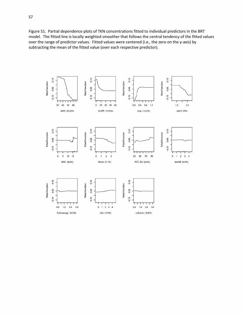
Figure S1. Partial dependence plots of TKN concentrations fitted to individual predictors in the BRT model. The fitted line is locally weighted smoother that follows the central tendency of the fitted values over the range of predictor values. Fitted values were centered (i.e., the zero on the y-axis) by subtracting the mean of the fitted value (over each respective predictor).

S8

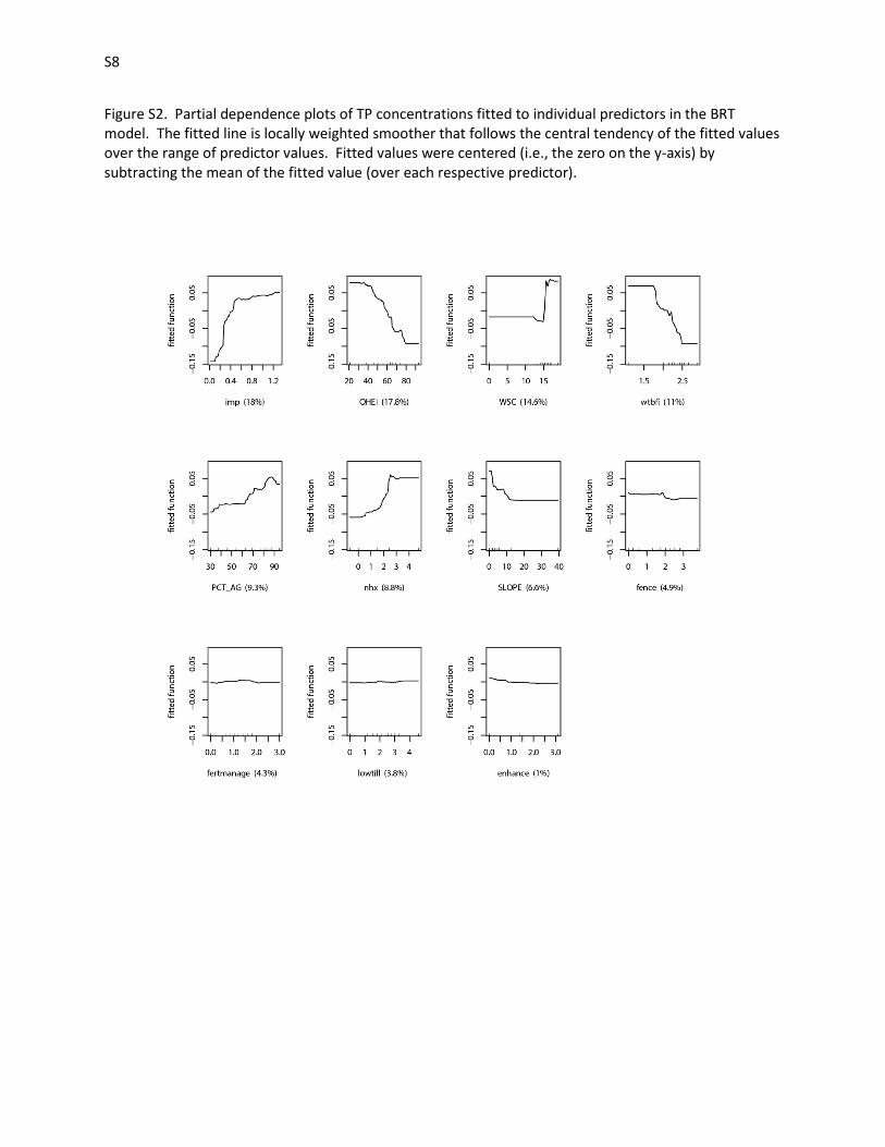
Figure S2. Partial dependence plots of TP concentrations fitted to individual predictors in the BRT model. The fitted line is locally weighted smoother that follows the central tendency of the fitted values over the range of predictor values. Fitted values were centered (i.e., the zero on the y-axis) by subtracting the mean of the fitted value (over each respective predictor).

S9

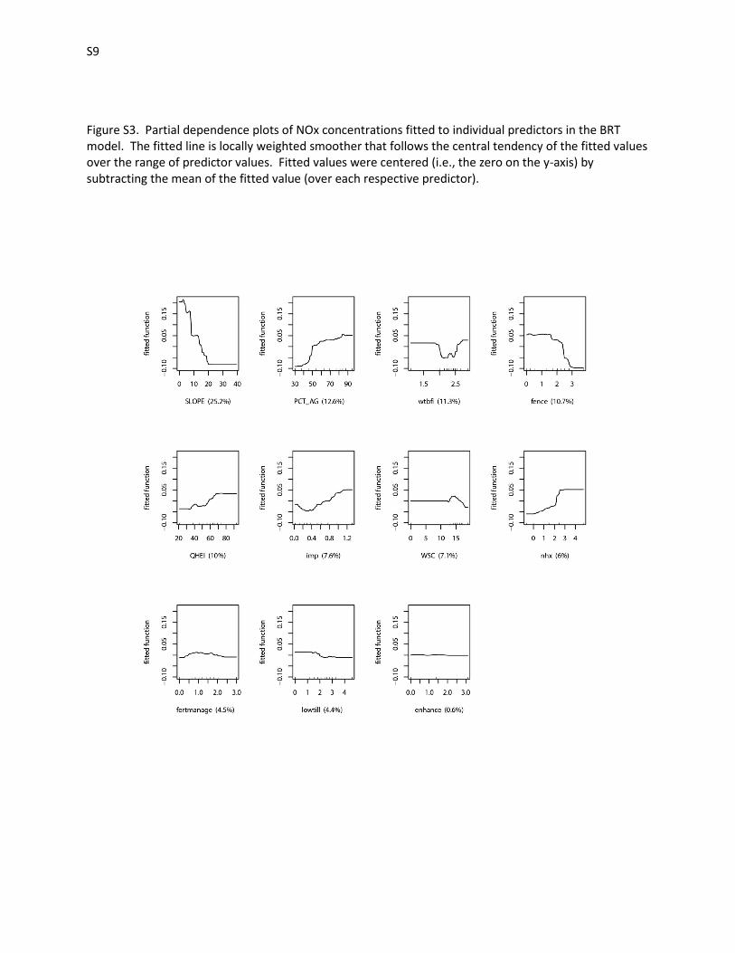
Figure S3. Partial dependence plots of NOx concentrations fitted to individual predictors in the BRT model. The fitted line is locally weighted smoother that follows the central tendency of the fitted values over the range of predictor values. Fitted values were centered (i.e., the zero on the y-axis) by subtracting the mean of the fitted value (over each respective predictor).

S10

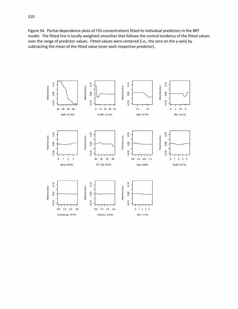
Figure S4. Partial dependence plots of TSS concentrations fitted to individual predictors in the BRT model. The fitted line is locally weighted smoother that follows the central tendency of the fitted values over the range of predictor values. Fitted values were centered (i.e., the zero on the y-axis) by subtracting the mean of the fitted value (over each respective predictor).

S11

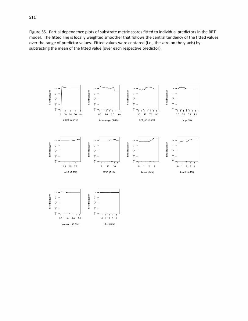
Figure S5. Partial dependence plots of substrate metric scores fitted to individual predictors in the BRT model. The fitted line is locally weighted smoother that follows the central tendency of the fitted values over the range of predictor values. Fitted values were centered (i.e., the zero on the y-axis) by subtracting the mean of the fitted value (over each respective predictor).

S12

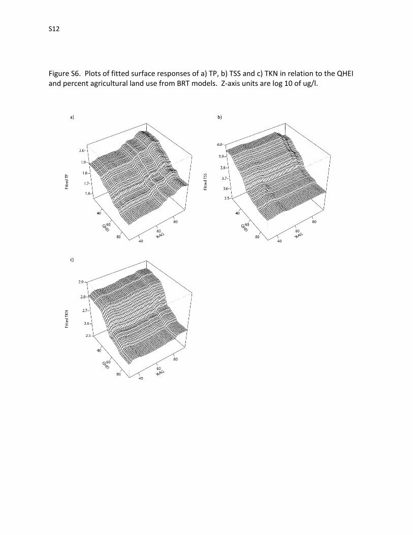
Figure S6. Plots of fitted surface responses of a) TP, b) TSS and c) TKN in relation to the QHEI and percent agricultural land use from BRT models. Z-axis units are log 10 of ug/l.