Supplementary Appendix to Government SpendingMultipliers in Good Times and in Bad: Evidence

from U.S. Historical Data

Valerie A. Ramey

University of California, San Diego and NBER

Sarah Zubairy

Texas A&M University

9 May 2017

Contents

1 Biases in computing multipliers 4

2 Robustness of slack estimates 4

3 Robustness of ZLB estimates 6

4 Behavior of taxes 7

5 Comparison with Auerbach-Gorodnichenko (2012) 9

6 Comparison with Auerbach-Gorodnichenko (2013) 13

7 Comparison with Fazzari, Morley and Panovska (2015) 13

List of Tables

1 Estimates of Multipliers Across States of Slack: Accounting for PresentValue Discounting . . . . . . . . . . . . . . . . . . . . . . . . . . . . . . 16

2 Robustness check I: Estimates of Multipliers Across States of Slack . . . . 173 Robustness check II: Estimates of Multipliers Across States of Slack . . . 184 Robustness checks I: Estimates of Multipliers Across Monetary Policy Regimes 195 Robustness checks II: Estimates of Multipliers Across Monetary Policy Regimes 206 Estimates of Multipliers Across Monetary Policy Regimes: Excluding World

War II and controlling for taxes and inflation . . . . . . . . . . . . . . . . 217 Comparison to Auerbach-Gorodnichenko (2012) Multipliers . . . . . . . . 228 Fazzari et al. (2015) Multipliers using the Jorda Method . . . . . . . . . . 23

List of Figures

1 Evolution of variables during war episodes . . . . . . . . . . . . . . . . . . 242 Government spending and GDP responses to a Blanchard-Perotti shock: Con-

sidering slack states . . . . . . . . . . . . . . . . . . . . . . . . . . . . . . 253 Cumulative multipliers to a Blanchard-Perotti shock: Considering slack states 26

2

4 Robustness check:Smooth transition threshold based on moving average ofoutput growth . . . . . . . . . . . . . . . . . . . . . . . . . . . . . . . . . 27

5 Taxes and Deficit Responses to a news shock: Considering linear model . . 286 State-dependent Taxes and Deficit Responses to a news shock: Considering

slack states . . . . . . . . . . . . . . . . . . . . . . . . . . . . . . . . . . 297 Government spending and GDP responses to a Blanchard-Perotti shock: Con-

sidering zero lower bound . . . . . . . . . . . . . . . . . . . . . . . . . . . 308 Cumulative multipliers with Blanchard-Perotti shock: Considering zero lower

bound . . . . . . . . . . . . . . . . . . . . . . . . . . . . . . . . . . . . . 319 Government spending and GDP responses to a news shock: Considering

zero lower bound and excluding World War II . . . . . . . . . . . . . . . . 3210 Cumulative multipliers with news shock: Considering zero lower bound and

excluding WWII . . . . . . . . . . . . . . . . . . . . . . . . . . . . . . . 3311 Cumulative multipliers with Blanchard-Perotti shock: Considering zero lower

bound and excluding WWII . . . . . . . . . . . . . . . . . . . . . . . . . 3412 Estimating Auerbach and Gorodnichenko (2012) State Dependent Responses

with the Jordà method . . . . . . . . . . . . . . . . . . . . . . . . . . . . . 3513 Government spending and GDP responses to a news shock: Considering

ZLB and Recessions in a Threshold-VAR . . . . . . . . . . . . . . . . . . 3614 Government spending and GDP responses to a Blanchard-Perotti shock: Con-

sidering ZLB and Recessions in a Threshold-VAR . . . . . . . . . . . . . . 37

3

1 Biases in computing multipliers

To determine whether using ex post conversion factors can lead to inflated multipliers, weconducted a test based on the following point made by Ramey (2013). If the contemporane-ous multiplier exceeds one, then it must be the case that private spending Y −G rises whenG rises. Thus, one can compare the multipliers estimated the standard way to the responseof real private spending to see if there is a contradiction.

To conduct this test, we first estimate a trivariate SVAR with military news, log realper capita government spending, and log real GDP, using four lags and quartic trend, on datafrom 1889 - 2015. The estimated elasticity at 2 year horizon is around 0.17 (based on the ratioof response of ln(Y) to response of ln(G) at 2 year horizon). We then multiply the estimatedelasticity by the average of Y/G for the full sample, and obtain an implied multiplier of 1.32.To conduct the comparison, we next estimate a model in which we substitute the log ofreal private spending for log real GDP, and compute the impulse response functions (usingthe standard method). These responses show that private spending falls when governmentspending rises, and specifically has a negative response at the 2 year horizon. Thus, theseresults imply a multiplier that is less than unity. It appears that the practice of backing outmultipliers using ex post conversion factors can lead to upward biased multiplier estimatesin some situations.

2 Robustness of slack estimates

Figure 2 shows the impulse responses using the Blanchard-Perotti shock. Figure 3 showsthe cumulative multipliers based on the Blanchard-Perotti shock for all horizons up to 20quarters.

We also conducted various additional robustness checks for both shocks. First, we com-pute multipliers using present values rather than simple sums. Table 1 shows that the resultsare very similar.

Second, we show the results for various transformations of the data. First, we follow Hall(2009) and Barro and Redlick (2011) in converting GDP and government spending changesto the same units before the estimation. In particular, our output and government spendingvariables on the left-hand-side are defined as (Yt+h − Yt−1)/Yt−1 and (Gt+h − Gt−1)/Yt−1. The

4

first variable can be rewritten as:

Yt+h − Yt−1

Yt−1≈ (lnYt+h − lnYt−1)

and hence is analogous to the standard VAR specification. The second variable can be rewrit-ten as:

Gt+h −Gt−1

Yt−1≈ (lnGt+h − lnGt−1) .

Gt−1

Yt−1

Thus, this variable converts the percent changes to dollar changes using the value of G/Y ateach point in time, rather than using sample averages. This means that the coefficients fromthe Y equations are in the same units as those from the G equations, which is required forconstructing multipliers. With this specification, we use a quartic trend and lags of loggedGDP and logged government spending on the right hand side. Table 2 shows that our baselineresults still hold. For the case of Blanchard and Perotti shocks, the multipliers are larger inmagnitude in the linear and state dependent case but there is no evidence of higher multipliersin high unemployment state.

The second panel of Table 2 also shows the results where in our baseline specification, weuse an alternative definition of trend GDP. We construct potential GDP using a cubic trendfor the early sample, fitted excluding Great Depression and append with the CBO potentialGDP measure for the available years. This alternative measure of potential GDP yields verysimilar multipliers to our baseline.

Also, we investigated the impact of using a different interpolation method for the data.Recall that our underlying interpolators were quite volatile and led to volatility in the earlydata. To investigate the impact, we create alternative data that uses linear interpolation ofthe annual data in the pre-WWII period. The top panel of Table 3 shows that the resultsfor the military news shock are little changed. Those for Blanchard-Perotti shock showslightly higher multipliers (0.5 to 0.6 in the linear case) and estimates that are virtually thesame across states. The four last panels of Table 3 show various other explorations, such asincluding trends, using Christina Romer’s estimates of historical GDP and unemployment,controlling for taxes and inflation, and controlling for trade-to-GDP ratios. The results aresimilar to the baseline.

5

3 Robustness of ZLB estimates

Tables 4 and 5 show various robustness checks for the ZLB state dependence case. When weconsider Hall-Barro-Redlick transformation for GDP and government spending, the multipli-ers are higher overall, particularly for Blanchard and Perotti shocks, but there is no evidenceof state-dependence. Using an alternative measure of trend GDP based on CBO potentialGDP measure yields results very similar to the baseline. When we consider linearly inter-polated data, the estimates for the ZLB state are slightly lower than the baseline case, andhigher at lower horizons in the normal state. For the Blanchard and Perotti shock the esti-mated multipliers are also higher in the normal state. The last panel shows that the results arealso similar to baseline for military shocks when we control for trade-to-GDP ratio. How-ever, the multipliers for the Blanchard and Perotti shock are larger than the baseline in thenormal case. While the addition of trends does not affect the military news shock results,the multipliers for the Blanchard and Perotti shock are larger than the baseline in the normalstate, in this case too. In fact, with the inclusion of trends, the multiplier in the normal statebecomes as large as the ZLB state at the 4 year horizon. In addition, Table 5 and Table 6show multiplier estimates for both the full sample and excluding WWII when taxes and in-flation are added as controls. The controls raise the multiplier estimates for the two-yearhorizon for the case of excluding WWII to 1.8, but the standard error is also higher and themultipliers are not statistically different across states.

Figure 9 shows the impulse responses for the baseline ZLB and normal states estimatedon the sample excluding WWII using military news shock. In contrast to the full sample(shown in the text), where government spending rises robustly beginning two quarters afterthe news shock in the ZLB state, in the sample excluding WII government spending becomesslightly negative for two quarters then slightly positive for two more quarters before begin-ning to rise robustly at horizon 5 with a peak at horizon 7. Output, however, rises steadilyas soon as the news hits and then jumps even higher at horizon 5. The delay in governmentspending after the news, along with the anticipation effect in GDP, shows up in the mul-tipliers in Figure 10. The estimated ZLB multipliers swing wildly from large negative tolarge positive with very wide confidence bands for the first few quarters, then reach 1.44 byhorizon 8. Recall from the text that the military news instrument rises above the relevancethreshold at horizon 5. At horizon 5, the multiplier is estimated to be 2.18 with a standard er-ror of 0.33. However, the IRFs demonstrate that the size of the multiplier stems from outputresponding more quickly to the news than government spending does.

6

4 Behavior of taxes

Our analysis did not explicitly study the responses of taxes. Table 3 shows that the multipliersdo not change when we control for taxes. However, the multipliers reported are based on theaverage response of taxes in the sample. Romer and Romer’s (2010) estimates of tax effectsindicate very significant negative multipliers on taxes, on the order of -2 to -3. Thus, it isimportant for us to consider how the increases in government spending are financed in orderto interpret our multiplier results.

To analyze how taxes and deficits behave, we re-estimate our basic model augmented toinclude deficits and tax rates so that we can distinguish increases in revenues caused by risingoutput versus rising rates. Average tax rates are computed as the ratio of federal receipts tonominal GDP. The deficit is the real total deficit. We include four lags of these two newvariables along with GDP and government spending as controls in all of the regressions, andwe estimate this system for the full sample using the Jordà method.

Figure 5 shows the results from the linear case. The responses of government spendingand GDP, as well as the multipliers, are almost identical to the baseline case. The middlepanels show that both average tax rates and the deficit increase in response to news shock.Taking the ratio of the cumulative response of deficit to cumulative response of governmentspending at various horizons, we estimate a sharp rise in the share of government spendingfinanced with the deficit during the first year. The deficit fraction of government spendingthen plateaus at 60 percent .

From a theoretical perspective, the fact that tax rates increase steadily during the first twoyears has significant implications for the multiplier. If all taxes are lump-sum taxes, newsabout a future increase in the present discounted value of government spending leads to animmediate jump in hours and output because of the negative wealth effect. In a neoclassicalmodel, the effect is the same whether the taxes are levied concurrently or in the future. Incontrast, the need to raise revenues through distortionary taxation can change incentivessignificantly. As Baxter and King (1993) show, if government spending is financed withcurrent increases in tax rates, the multiplier can become negative in a neoclassical model.

The situation changes considerably when tax rates are slow to adjust, but agents antic-ipate higher future tax rates. To see this, consider the case of labor income taxes and aforward-looking household:

(1) 1 = βEt

[un,t+1

un,t

(1 − τt)wt

(1 − τt+1)wt+1(1 + rt)

]7

where un is the marginal utility of leisure, τ is the tax on labor income, w is the real wagerate, r is the real interest rate, and Et is the expectation based on period t information. Inexpectation, the household should vary the growth rate of leisure inversely with the growthrate of after-tax real wages. This means that if τt+1 is expected to rise relative to τt, house-holds have an incentive to substitute their labor to the present (when it is taxed less) and theirleisure to the future.

It is easy to show in a standard neoclassical model that the delayed response of taxes, suchas we observe in the estimated impulse responses, results in a multiplier that is higher in theshort-run but lower in the long-run relative to the lump-sum tax case. We have also conductedthis experiment in the Gali et al. (2007) model where 50 percent of the households are rule-of-thumb consumers. We found the same effect in that model as well. Drautzburg andUhlig (2015) analyze an extension of the Smets-Wouters model and also find that the timingof distortionary taxes is very important for the size of the multiplier. Given the impulseresponse of tax rates, and with these theoretical results in mind, it is very possible that ourestimated multipliers are greater than we would expect if taxation were lump-sum.

Nevertheless, our finding that multipliers do not vary across states could be due to dif-ferential financing patterns. To determine whether this is the case, Figure 6 shows the state-dependent results in response to a news shock. As we showed before, both governmentspending and GDP rise more if a news shock hits during a slack state, even after adjustingthe initial size of the shock. The bottom panels show that tax rates and deficits also rise moreduring recessions, but there are other interesting differences in the patterns. When we studythe ratio of the cumulative deficit to cumulative government spending at each point in timealong the path, we find that more of government spending is financed with deficits when ashock hits during a slack state.1 For example, at quarter seven the ratio of the cumulativedeficit to cumulative government spending is 61 percent if a shock hits during a slack statebut only about 45 percent if the shock hits during a non-slack state. Thus, on average short-run government spending is financed more with deficits if the shock hits during a slack state.In addition, tax rates rise with a delay during the slack state relative to non-slack state. Thiswould imply that the multiplier should be greater during times of slack. In fact, our estimatesimply that it is not.

1. This is true with the exception of the second quarter. This can be explained by the fact that initiallygovernment spending and deficits rise slowly in response to a news shock and and for the initial two quarters,deficits fall very slightly before rising.

8

5 Comparison with Auerbach-Gorodnichenko (2012)

This section discusses the details of the results we mentioned in the text in our discussionof Auerbach and Gorodnichenko’s (2012) (AG-12) method. AG-12 use a smooth transitionVAR (STVAR) model, post-WWII data, the Blanchard-Perotti identification method, and afunction of the 7-quarter centered moving average of normalized real GDP growth as theirmeasure of the state. They use three lags of the endogenous variables in the VAR, but alsoinclude four lags of the 7-quarter moving average growth rate as exogenous regressors intheir model.2 They construct their baseline impulse responses based on two assumptions:(1) the economy remains in an extreme recession or expansion state for at least 5 years; and(2) changes in government spending do not impact the state of the economy.3 They findmultipliers during recessions that are well above two and these results have been cited bythose advocating stimulus during the Great Recession (e.g. DeLong and Summers (2012))

To understand the difference between our results and theirs, we begin by taking only onestep away from what AG-12 did by using all details of their analysis except the method forestimating and constructing the impulse responses. In particular, we apply the Jordà methodto their post-WWII data, using their exact definition of states, logs of variables, estimatedgovernment spending shocks from their STVAR model, and inclusion of four lagged valuesof the centered 7-quarter moving average of output growth as controls. F(z) is the indicatorof the state as a function of the moving average of output (z). It varies between a maximumof one (extreme recession) and zero (extreme expansion).

The top panel of Figure 12 reproduces the impulse responses shown in Figure 2 fromAG-12. They construct these impulse responses from their STVAR estimates, assuming thatthe economy does not switch states for at least 20 quarters. The second panel shows the lin-ear responses estimated using the Jordà method.4 The government spending response lookssimilar to the linear case in AG-12, though the GDP response is more erratic and the stan-dard error bands are much wider. The state-dependent responses shown in the lower panellook very different. The Jordà method produces impulse responses in which the response ofgovernment spending to a shock is higher in a recession than in an expansion, similar to ourearlier results, but in opposition to those of AG-12. The response of output differs little across

2. The published paper does not discuss these additional terms, but the initial working paper version includesthese terms in one equation and the codes posted for the published paper include them.

3. These results are shown in Table 1 and Figure 2 of their paper.4. We have multiplied the log output response by a conversion factor of 5.6, following AG-12. They use a

nonstandard measure of government purchases as their measure of G. As a result their Y/G ratio used to convertmultipliers is higher than the usual one based on total government purchases.

9

states, in contrast to AG-12 who find that output rises robustly and continuously throughoutthe 5 years in the recession state but quickly falls toward zero and becomes negative in theexpansion state.

The first panel of Table 7 compares AG-12’s cumulative 5-year and 2-year multipliersto those we estimated by the Jordà method. For the 5-year horizon, AG find multipliers of2.24 for recessions and -0.33 for expansions whereas the Jordà method estimates multipliersof 0.84 in recessions and -0.59 in expansions.5 Thus, the Jordà multipliers are below onein recessions, but similar to AG-12’s multipliers in expansions. At the 2-year horizon, AG’sestimates imply a recession multiplier of 1.65 and a gap between states of 1.55. In contrast,the Jordà method implies a 2-year multiplier in recessions of 0.24 and a gap between statesof -0.12.6

Thus, even when we use the same sample period, data, variable definitions, definition ofslack, and estimated shocks as AG-12, the Jordà method produces multipliers in recessionsthat are much lower than those of AG-12. This means that AG-12’s high multipliers duringrecessions are likely due to the method for constructing the impulse responses. To see theimportance of these assumptions, we conduct several experiments. In these experiments, wecompute alternative impulse responses by iterating on AG’s STVAR parameter estimates un-der different assumptions about the dynamics of the state of the economy. Since the economyis never literally in an extreme recession or expansion, we focus on the average of "severe"recessions and "severe" expansions, which we define as the few quarters in which F(z) isabove 0.95 or below 0.05, respectively. The few quarters of severe recession occur duringthe recessions of 1974-75 (two quarters), 1981-82 (one quarter), and 2008-09 (five quarters).

The second panel of Table 7 reports these experiments. For reference, the first line ofthe second panel shows that AG’s baseline 5-year multipliers do not change much when wechange F(z) by a small amount. The second line shows the multiplier calculated assuming aconstant state and no feedback, but looking at the 2-year integral multiplier. This calculationrequires less drastic assumptions because it only assumes that the state remains constant for2 years rather than 5 years. Here, the multipliers in severe recessions are not as high andthose in severe expansions are not as low, so the difference across states falls from 2.47 to1.46.

The next experiment, "Actual State Dynamics," assumes that instead of staying constant

5. AG-12 also report a recession multiplier of 2.5, but that is based on comparing the peak response of outputto the initial government spending shock, a practice we critiqued in a previous section.

6. One should keep in mind, however, that the Jordà estimates are not very precise. We were not able toestimate the standard errors of the multipliers because the xtscc command in Stata reported that the variancematrix was nonsymmetric or highly singular.

10

at an extreme value, the state indicator F(z) is equal to its actual value at each point intime. In practice the experiment is conducted as follows. We first calculate the paths ofgovernment spending and output, assuming that the shocks to the government spending,tax, and output equations take their estimated values. This essentially reproduces the actualpath of the economy for all variables including F(z). We then calculate an alternative pathof government spending, taxes, and output assuming that there is an additional one-timepositive shock in the current period to government spending, equal to one standard deviationof the estimated government spending shock (equal to 1.3 percent of government spending).We allow the shock to change the path of spending, taxes, and output, but not the state ofthe economy, F(z), relative to its actual path. The difference between this simulation andthe actual values of the variables forms the impulse response functions. Despite the lack offeedback, this experiment is different from AG’s baseline experiment because it allows thestate of the economy to experience its natural dynamics (i.e. F(z) is allowed to vary betweenits extremes as it actually does).7 The third and fourth lines of the lower panel show themultipliers for this experiment. In severe recessions, the 5-year multiplier is estimated to be1.4 and the 2-year multiplier is estimated to be 1.1. Thus, allowing the state of the economyto follow its subsequent natural dynamics reduces the constructed multiplier in recessions.The effect is not so big on the expansion multipliers, however. This is to be expected sinceexpansions have a much longer duration than recessions, so the assumption of no change instate is not so at odds with the data.

AG-12 relax one of their baseline assumptions in a second experiment by allowing partialfeedback of government spending on the state of the economy, but otherwise not allowingthe state to change. They are not able to allow full feedback, though, because of the nature oftheir state variable.8 The fifth and sixth lines of the second panel of the table show the averageof their multipliers in severe recessions and expansions. Their experiment also lowers theestimated multiplier in severe recessions, to 1.36 for the 5-year multiplier and 1.01 for the2-year multiplier.

The final two lines of the table show our experiment in which we allow both the naturaldynamics of the economy and partial feedback from the government spending shock. The

7. The assumptions regarding the state F(z) are important. For instance, Caggiano et al. (2015) employ theSTVAR approach of AG-12 for a shorter sample, but compute impulse response functions using the generalizedimpulse response approach advocated by Koop et al. (1996), and find that the spending multipliers in recessionsare not statistically larger than in expansions. They only find evidence of nonlinearities when focusing on deeprecessions versus strong expansionary periods.

8. Their state variable is a function of a centered moving average of GDP growth. Thus, future values of GDPenter the current state. This formulation makes it impossible to allow full feedback in a logically consistentmanner.

11

experiment is the same as the "Actual State Dynamics, No Feedback" except that it also al-lows the F(z) indicator to change from its actual path in reaction to current changes of outputresulting from the government spending shock. As shown in the table, both the 5-year and2-year multipliers during severe recessions are calculated to be 1.07. During severe expan-sions, the 5-year multiplier is calculated to be 0.14, which is higher than AG’s multiplier of-0.3. As a result, the gap in multipliers across states shrinks.

Thus, even when we use AG’s STVAR parameter estimates, we can get very differentestimates for the multiplier. Differing assumptions made about transitions between statesand the feedback of government spending to the state lead to very different estimates ofmultipliers. When we compute multipliers allowing for the natural dynamics of the economywe find a much smaller gap across states than AG-12. The gap we do find is not becausethe multiplier is so high during recessions, but because it is estimated to be so low duringexpansions when we use AG’s data and variable definitions.

As pointed out above, the state variable that AG-12 employ is a function of a centered

moving average of GDP growth. This suggest that future values of GDP are used to constructthe current state of the economy. This formulation not only makes it impossible to allow fullfeedback in a logically consistent manner, but it in fact plays an important role in drivingtheir results as well. In our exploration of the AG-12 results, we found that if we focus onlyon the backward moving average terms, and in particular, instead of a 7-quarter centeredmoving average growth rate, consider a 4-quarter backward moving average growth rate,while keeping all the details of the AG set-up the same, the resulting multiplier is muchlarger in expansion than in recession.9 Alloza (2014) conducts a much more systematicanalysis of the importance of this two-sided moving average filter and further corroboratesour finding. He finds that using a higher order of centered moving average (i.e. using moreinformation about future values of GDP) reduces the effect of the spending shock on outputduring times of booms and amplifies it during recession periods. He also explores varyingthe symmetry of the 7-quarter moving average, and shows that when less information aboutthe future is used, then the results suggest a more robust response of output to a spendingshock in booms, while the response in recessions becomes negative. This suggests, that thefuture information used in constructing the current state variable in AG-12 is also crucial totheir results.

9. The 5 year cumulative multiplier is close to 0.7 in recession and 1.8 in expansion.

12

6 Comparison with Auerbach-Gorodnichenko (2013)

Auerbach-Gorodnichenko (AG-13) also applies the Jordà method to a panel of OECD coun-tries; in fact, AG-13 were the ones who first realized the potential of this method for state-dependent fiscal models. Thus, a key question is why they find higher multipliers duringrecessions even with this method. There is, of course, the obvious difference in time periodand country sample. We believe, however, the most likely reason for the difference is in twodetails of how they calculate multipliers. First, following the standard practice, they estimateeverything in logarithms and then use the ex post conversion factor based on average Y/G

during their sample to convert elasticities to multipliers. Second, they follow Blanchard andPerotti (2002) by comparing the path or peak of output to the impact of government spend-ing rather than to the peak or integral of the path of government spending. This is a bigdifference because the effects of a shock to government usually build up for several quarters.As we argued in a previous section, this is not the type of multiplier that interests policymakers because it does not count the average cumulative cost of government spending asso-ciated with the path. If we used that same procedure on our baseline estimates, calculatingmultipliers by dividing the average response of output over the 2-year horizon by the initial

shock to government spending, we would produce multipliers of 4.3 in the linear case, 2.2in the low unemployment state and 8.8 in the high unemployment state! Thus, it is clear thateven using the same estimation method and same method for computing impulse responses,details of the calculations of multipliers can make a big difference.

7 Comparison with Fazzari, Morley and Panovska (2015)

Fazzari et al. (2015) estimate a threshold structural VAR and extend Auerbach and Gorod-nichenko’s (2012) work in three key ways: (i) they estimate multipliers based on generalizedimpulse responses functions; (ii) they investigate a variety of measures of slack; and (iii)they estimate the threshold for each measure rather than imposing it a priori. Based on a se-ries of statistical tests, they use their own structural break-adjusted capacity utilization indexand estimate their model from 1967-2012. They find evidence of a higher multiplier, of 1.6,in the slack state, defined as a structural break-adjusted capacity utilization rate below theirestimated threshold.

To understand the difference between our results and theirs, we begin by taking only onestep away from what they did by using all details of their analysis except the method for

13

estimating and constructing the impulse responses. In particular, we employ their samplechoice, identification scheme, specification of variables and threshold variables along withthe estimated threshold values, but use the Jorda methodology to estimate the multipliers. Weconduct this exercise for their baseline specification that uses their structural break-adjustedcapacity utilization measure as the state variable; this measure subtracts a different meanfor the 1967-1974 sample than for the post-1974 sample and this adjustment affects theestimated threshold for the entire sample. We also conduct this exercise for the other slackvariables identified in their Table 2 that have marginal likelihoods close in size to the bestfitting model.

Table 8 shows the implied multipliers. The first panel shows that when we use their pre-ferred threshold variable of adjusted capacity utilization, we also estimate larger multipliersin the slack state. At the 2-year horizon, it is as large as 2.5 and statistically significantlydifferent from the multiplier in the high capacity utilization state. Thus, our data and methodproduce even higher multipliers than they find. But then we consider their other slacknessmeasures, i.e. the standard series on capacity utilization (without their 1967-1974 mean ad-justment), the CBO output gap, and the unemployment rate as slack variables, using theirthreshold estimates. These results show that we no longer find any evidence of higher multi-pliers in the slack state, and in fact, in the case of unadjusted capacity utilization, the multi-pliers are negative in the slack state. The only case where we find higher multipliers in slackis the case of the unemployment rate threshold, but the multipliers are much smaller than oneunder both states, not statistically significantly different across states and the point estimatedifference in the long run is driven by multipliers being low in the non-slack state. These re-sults suggest that the multipliers produced by the Fazzari et al. (2015) method are not robustto closely-related slack measures and are highly dependent on the specific choice of thresh-old variable and threshold estimate. Multipliers estimated using these close alternatives tothe slack index are not shown in their paper.

Thus, the only one of their high marginal likelihood slack measures that produces highmultipliers in recessions is the capacity utilization series that they adjust for a structural breakin 1974q1. This adjustment, along with their estimated threshold, reassigns 20 percent of thesample to a different state relative to the standard capacity utilization index and threshold.We investigated several aspects of this series. First, we found that their structural break-adjusted capacity utilization index has a lower correlation with the CBO output gap than theunadjusted capacity utilization index (0.6 vs. 0.8). Second, when we tested their series for asingle structural break, we found a break at 2001q1, not 1974q1. This break date held in tests

14

that trimmed the standard 15 percent of each end of the sample (which excludes early 1974)as well as in those that trimmed 5 and 10 percent. It also held for both the supremum Waldtest and the supremum likelihood ratio test. We also tested a series on capacity utilization inmanufacturing, since that series looks very similar to the total series but has the advantagethat it is available back to 1948. A structural break test on that series found a break at2000q4. These auxiliary tests raise questions about the structural break-adjusted series usedby Fazzari et al. (2015), and hence the estimated multipliers associated with that series.

15

Table 1. Estimates of Multipliers Across States of Slack: Accounting for Present ValueDiscounting

Linear High LowModel Unemployment Unemployment

BaselineMilitary news shocks2 year integral 0.70 0.43 0.694 year integral 0.71 0.56 0.60

Blanchard-Perotti shocks2 year integral 0.53 0.74 0.454 year integral 0.60 0.81 0.42

Present discounted value multipliersMilitary news shocks2 year integral 0.71 0.40 0.714 year integral 0.71 0.59 0.57

Blanchard-Perotti shocks2 year integral 0.51 0.73 0.444 year integral 0.60 0.80 0.42

Note: The multipliers are computed for the sub-sample 1920-2015, where the discount factor isconstructed using the T-bill rate and past inflation.

16

Table 2. Robustness check I: Estimates of Multipliers Across States of Slack

Linear High LowModel Unemployment Unemployment

Hall-Barro-Redlick transformationMilitary news shock2 year integral 0.76 0.75 0.824 year integral 0.83 0.79 0.97Blanchard-Perotti shock2 year integral 0.57 0.69 0.484 year integral 0.93 0.82 1.02

Alternative definition of potential GDP based on CBO measureMilitary news shock2 year integral 0.67 0.61 0.644 year integral 0.71 0.69 0.68Blanchard-Perotti shock2 year integral 0.39 0.70 0.32†

4 year integral 0.48 0.79 0.35†

Note: The symbol on the last entry in each row signifies the p-values for difference in multipliersacross state, where † indicates HAC-robust p-value, pHAC < 0.1.

17

Table 3. Robustness check II: Estimates of Multipliers Across States of Slack

Linear High LowModel Unemployment Unemployment

Linearly interpolated dataMilitary news shock2 year integral 0.66 0.67 0.534 year integral 0.69 0.72 0.57Blanchard-Perotti shock2 year integral 0.51 0.42 0.474 year integral 0.58 0.57 0.53

Addition of trendsMilitary news shock2 year integral 0.77 0.70 0.614 year integral 0.85 0.75 0.72Blanchard-Perotti shock2 year integral 0.46 0.70 0.42†

4 year integral 0.62 0.82 0.53†

Christina Romer series for GDP, PGDP and UNEMPMilitary news shock2 year integral 0.66 0.49 0.614 year integral 0.69 0.62 0.61Blanchard-Perotti shock2 year integral 0.40 0.67 0.33†

4 year integral 0.48 0.723 0.34†

Additional controls for taxes and inflationMilitary news shock2 year integral 0.67 0.66 0.564 year integral 0.71 0.69 0.60Blanchard-Perotti shock2 year integral 0.38 0.67 0.37†

4 year integral 0.44 0.79 0.40†

Additional controls for trade-to-GDP ratioMilitary news shock2 year integral 0.66 0.60 0.594 year integral 0.71 0.68 0.67Blanchard-Perotti shock2 year integral 0.38 0.68 0.304 year integral 0.47 0.77 0.35

Note: The symbol on the last entry in each row signifies the p-values for difference in multipliersacross state, where † indicates HAC-robust p-value, pHAC < 0.1.

18

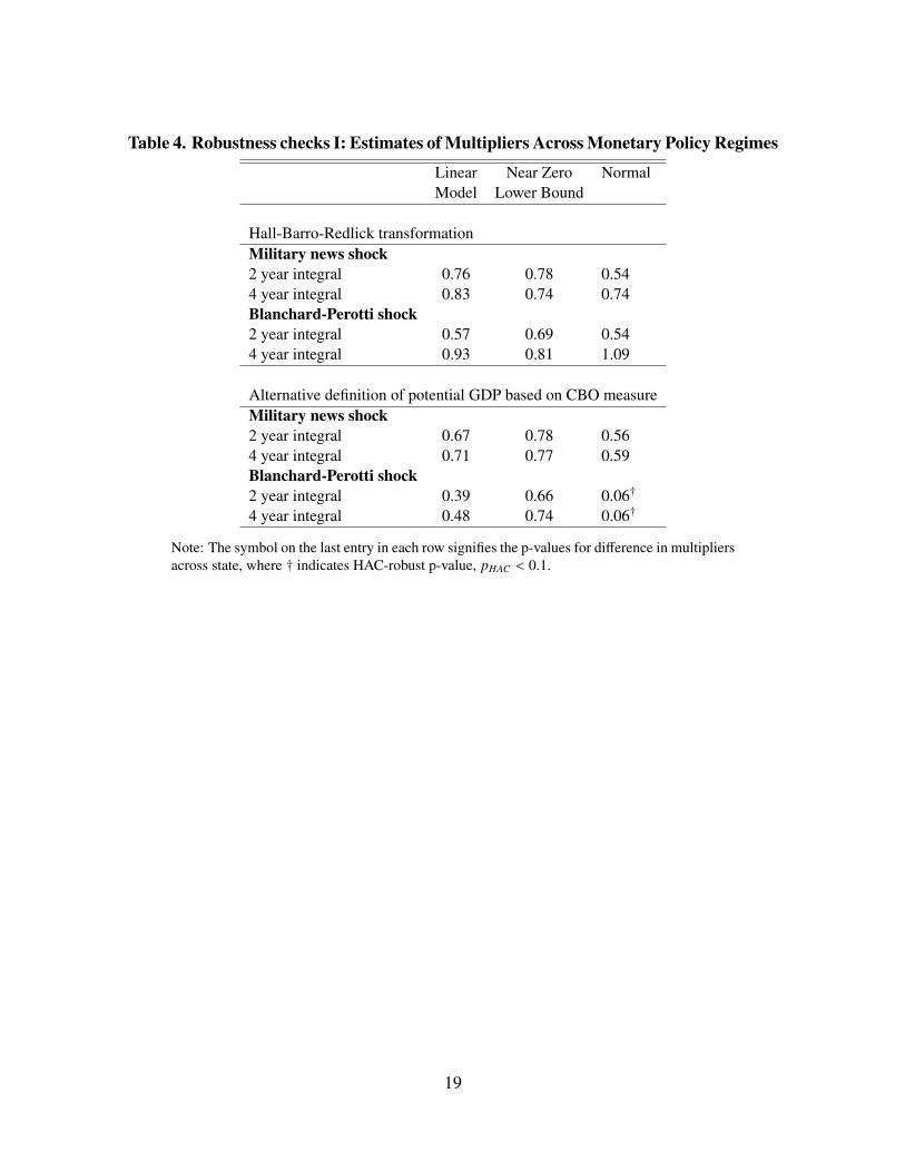
Table 4. Robustness checks I: Estimates of Multipliers Across Monetary Policy Regimes

Linear Near Zero NormalModel Lower Bound

Hall-Barro-Redlick transformationMilitary news shock2 year integral 0.76 0.78 0.544 year integral 0.83 0.74 0.74Blanchard-Perotti shock2 year integral 0.57 0.69 0.544 year integral 0.93 0.81 1.09

Alternative definition of potential GDP based on CBO measureMilitary news shock2 year integral 0.67 0.78 0.564 year integral 0.71 0.77 0.59Blanchard-Perotti shock2 year integral 0.39 0.66 0.06†

4 year integral 0.48 0.74 0.06†

Note: The symbol on the last entry in each row signifies the p-values for difference in multipliersacross state, where † indicates HAC-robust p-value, pHAC < 0.1.

19

Table 5. Robustness checks II: Estimates of Multipliers Across Monetary PolicyRegimes

Linear Near Zero NormalModel Lower Bound

Linearly interpolated dataMilitary news shock2 year integral 0.66 0.66 0.374 year integral 0.69 0.69 1.03Blanchard-Perotti shock2 year integral 0.51 0.61 0.314 year integral 0.58 0.69 0.35

Addition of trendsMilitary news shock2 year integral 0.77 0.78 0.654 year integral 0.85 0.78 0.86Blanchard-Perotti shock2 year integral 0.46 0.64 0.334 year integral 0.62 0.71 0.75

Additional controls for inflationMilitary news shock2 year integral 0.67 0.77 0.604 year integral 0.71 0.77 0.58Blanchard-Perotti shock2 year integral 0.38 0.65 0.08†

4 year integral 0.46 0.72 0.09†

Additional controls for taxes and inflationMilitary news shock2 year integral 0.67 0.94 0.554 year integral 0.71 0.86 0.52Blanchard-Perotti shock2 year integral 0.38 0.67 0.08†

4 year integral 0.44 0.74 −0.02†

Additional controls for trade-to-GDP ratioMilitary news shock2 year integral 0.66 0.76 0.634 year integral 0.71 0.75 0.78Blanchard-Perotti shock2 year integral 0.38 0.64 0.104 year integral 0.47 0.70 0.12

Note: The symbol on the last entry in each row signifies the p-values for difference in multipliersacross state, where † indicates HAC robust p-value pHAC < 0.1.20

Table 6. Estimates of Multipliers Across Monetary Policy Regimes: Excluding WorldWar II and controlling for taxes and inflation

Linear Near Zero Normal P-value for differenceModel Lower Bound in multipliers across

Military news shock2 year integral 0.80 1.73 0.55 HAC =0.005

(0.236) (0.317) (0.128) AR =0.154

4 year integral 0.74 0.90 0.52 HAC = 0.154

(0.170) (0.159) (0.224) AR =0.174

Blanchard-Perotti shock2 year integral 0.06 0.85 0.08 HAC = 0.110

(0.159) (0.439) (0.187) AR =0.173

4 year integral -0.07 -0.63 −0.02 HAC = 0.711

(0.275) (1.57) (0.252) AR =0.640

Note: The values in brackets under the multipliers give the standard errors. HAC indicatesHAC-robust p-values and AR indicates weak instrument robust Anderson-Rubin p-values.

21

Table 7. Comparison to Auerbach-Gorodnichenko (2012) Multipliers

Direct Comparisons Extreme ExtremeRecession Expansion(F(z)=1) (F(z)=0) Difference

AG’s Estimates, Constant State5 year integral 2.24 -0.33 2.57

(0.24) (0.20)2 year integral 1.65 0.10 1.55

Jordà Method Applied to AG Specification5 year integral 0.84 -0.59 1.432 year integral 0.24 0.36 -0.12

Alternative Multipliers Severe Severeusing Recession ExpansionAG’s STVAR Estimates (F(z) ≥ 0.95) (F(z) ≤ 0.05) Difference

Constant State, No Feedback5 year integral 2.16 -0.31 2.472 year integral 1.56 0.10 1.46

Actual State Dynamics, No Feedback5 year integral 1.41 0.19 1.222 year integral 1.13 0.15 0.97

AG Partial Feedback5 year integral 1.36 -0.04 1.402 year integral 1.01 0.15 0.86

Actual State Dynamics, Partial Feedback5 year integral 1.07 0.14 0.932 year integral 1.07 0.12 0.95

Note: STVAR denotes the Smooth Transition Vector Autoregression used by AG-12. Impulseresponses are calculated based on the VAR parameter estimates and auxiliary assumptions. Thevalues in brackets under the multipliers give the standard errors. F(z) is AG’s indicator of thestate of the economy. F(z) = 1 indicates the most severe recession possible and F(z) = 0 indicatesthe most extreme boom possible."Constant state" means that the impulse responses are calculated assuming that the economyremains in its current state for the duration of the multiplier. "Feedback" means that the estimatesallow government spending to change the state of the economy going forward.

22

Table 8. Fazzari et al. (2015) Multipliers using the Jorda Method

Linear Slack Non-SlackModel State State

Capacity utilization (adjusted)2 year integral 0.31 2.55 0.13†

4 year integral -0.50 1.33 −0.44

Capacity utilization2 year integral 0.31 -0.65 1.344 year integral -0.50 -1.41 -0.32

Output gap2 year integral 0.31 0.69 0.964 year integral -0.50 0.19 -0.31

Unemployment rate2 year integral 0.31 0.58 0.364 year integral -0.50 0.13 -1.38

Note: We use all details of Fazzari et. al (2015) analysis including the sample choice, identi-fication scheme, specification of variables, threshold variable along with the threshold estimatebut use the Jorda methodology to get the multipliers. The symbol on the last entry in each rowsignifies the p-values for difference in multipliers across state, where † indicates HAC-robustp-value, pHAC < 0.1.

23

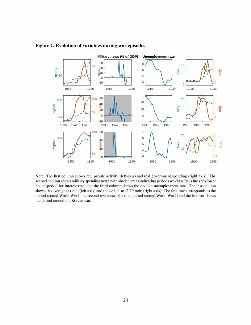
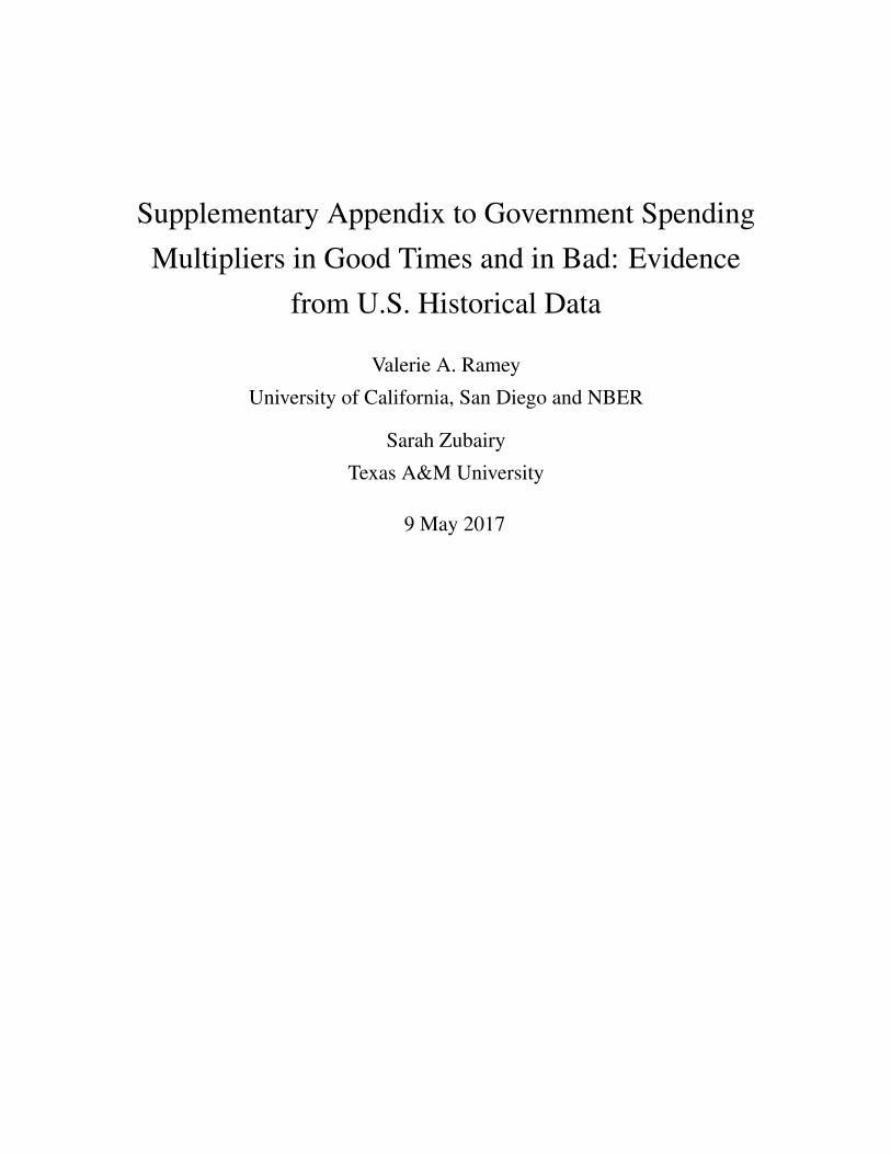
Figure 1. Evolution of variables during war episodes

1915 1920

nypr

iv

50 ngov

20

1915 1920

-10

0

10

20

30

Military news (% of GDP)

1915 1920

2

4

6

8

Unemployment rate

1915 1920

taxy

0

10

defy

0

1938 1942 1946

nypr

iv

100

200ng

ov

50

100

1938 1942 1946-20

0

20

40

60

1938 1942 1946

5

10

15

1938 1942 1946

taxy

20

defy

0

1950 1955

nypr

iv

300

ngov

50

100

1950 1955

0

20

40

60

1950 1955

3

4

5

6

7

1950 1955

taxy

15

20

defy

-5

0

5

Note: The first column shows real private activity (left-axis) and real government spending (right axis). Thesecond column shows military spending news with shaded areas indicating periods we classify as the zero lowerbound period for interest rate, and the third column shows the civilian unemployment rate. The last columnshows the average tax rate (left axis) and the deficit-to-GDP ratio (right axis). The first row corresponds to theperiod around World War I, the second row shows the time period around World War II and the last row showsthe period around the Korean war.

24

Figure 2. Government spending and GDP responses to a Blanchard-Perotti shock:Considering slack states

5 10 15 20

Gov

ernm

ent s

pend

ing

0

1

2

3

5 10 15 200

1

2

3

Linear

5 10 15 20

0

1

2

3

4

5State-dependent

quarter5 10 15 20

GD

P

0

0.5

1

1.5

2

2.5

quarter5 10 15 20

0

0.5

1

1.5

2

quarter5 10 15 20

0

1

2

3

4

Linear

Low Unemp

High Unemp

Note: Response of government spending and GDP to a 1% of government spending shock. The top row showsthe response of government spending and the second row shows the response of GDP. The first column showsthe responses in the linear and state-dependent model. The second column shows the responses in the linearmodel. The last column shows the state-dependent responses where the blue dashed lines are responses in thehigh unemployment state and the lines with red circles are responses in the low unemployment state. 95%confidence intervals are shown in second and third columns.

25

Figure 3. Cumulative multipliers to a Blanchard-Perotti shock: Considering slackstates

2 4 6 8 10 12 14 16 18 20

0

0.1

0.2

0.3

0.4

0.5

0.6

0.7Linear: cumulative spending multiplier

quarter2 4 6 8 10 12 14 16 18 20

-0.2

0

0.2

0.4

0.6

0.8

State dependent: cumulative spending multiplier

Note: Cumulative spending multipliers across different horizons. The top panel shows the cumulative mul-tipliers in the linear model. The bottom panel shows the state-dependent multipliers where the blue dashedlines are multipliers in the high unemployment state and the lines with red circles are multipliers in the lowunemployment state. 95% confidence intervals are shown in all cases.

26

Figure 4. Robustness check:Smooth transition threshold based on moving average ofoutput growth

1900 1920 1940 1960 1980 2000

0.1

0.2

0.3

0.4

0.5

0.6

0.7

0.8

0.9

Note: The figures shows the weight on a recession regime, which is constructed using the 7 quarter centeredmoving average of output growth and the same definition as Auerbach and Gorodnichenko (2012). The shadedareas indicate NBER official recessions.

27

Figure 5. Taxes and Deficit Responses to a news shock: Considering linear model

5 10 15 20

0

0.1

0.2

0.3

0.4

0.5

Government spending

5 10 15 200

0.1

0.2

0.3

0.4

GDP

5 10 15 200

0.02

0.04

0.06

0.08

0.1

Taxes

5 10 15 20

0

0.1

0.2

0.3

Deficit

quarter5 10 15 20

0

0.1

0.2

0.3

0.4

0.5

Ratio of cumulative deficit to cumulative spending

Note: These are responses for taxes and deficits in the linear model. The shaded areas indicate 95% confidencebands.

28

Figure 6. State-dependent Taxes and Deficit Responses to a news shock: Consideringslack states

5 10 15 20

0

0.2

0.4

0.6

0.8

1 Government spending

5 10 15 20

0

0.2

0.4

0.6

0.8 GDP

5 10 15 20

0

0.05

0.1

0.15

0.2

Taxes

5 10 15 20

0

0.2

0.4

Deficit

quarter5 10 15 20

-1

-0.5

0

0.5

Ratio of cumulative deficit to cumulative spending

Note: These are state-dependent responses for taxes and deficits, where the black solid lines are responses inthe high unemployment state and the lines with red circles are responses in the low unemployment state. 95%confidence intervals are also shown.

29

Figure 7. Government spending and GDP responses to a Blanchard-Perotti shock:Considering zero lower bound

5 10 15 20

Gov

ernm

ent s

pend

ing

0

0.5

1

1.5

2

2.5

5 10 15 200

1

2

3

Linear

5 10 15 20

0

1

2

3

4State-dependent

quarter5 10 15 20

GD

P

0

0.5

1

1.5

quarter5 10 15 20

0

0.5

1

1.5

2

quarter5 10 15 20

0

1

2

Linear

ZLB

Normal

Note: Response of government spending and GDP to a 1% of government spending shock. The top row showsthe response of government spending and the second row shows the response of GDP. The first column showsthe responses in the linear and state-dependent model. The second column shows the responses in the linearmodel. The last column shows the state-dependent responses where the blue dashed lines are responses in thenear zero-lower bound state and the lines with red circles are responses in the normal state. 95% confidenceintervals are shown in second and third columns.

30

Figure 8. Cumulative multipliers with Blanchard-Perotti shock: Considering zerolower bound

2 4 6 8 10 12 14 16 18 20

0

0.1

0.2

0.3

0.4

0.5

0.6

0.7Linear: cumulative spending multiplier

quarter2 4 6 8 10 12 14 16 18 20

-0.2

0

0.2

0.4

0.6

0.8

State dependent: cumulative spending multiplier

Note: Cumulative spending multipliers across different horizons for a Blanchard-Perotti shock. The top panelshows the cumulative multipliers in the linear model. The bottom panel shows the state-dependent multiplierswhere the blue dashed lines are multipliers in the near zero-lower bound state and the lines with red circles aremultipliers in the normal state. 95% confidence intervals are shown in all cases.

31

Figure 9. Government spending and GDP responses to a news shock: Considering zerolower bound and excluding World War II

quarter5 10 15 20

-0.1

0

0.1

0.2

0.3

0.4

0.5

0.6

0.7

State dependent: Government spending

quarter5 10 15 20

-0.2

-0.1

0

0.1

0.2

0.3

State dependent: GDP

Note: Response of government spending and GDP to a news shock equal to 1% of GDP. The figure shows thestate-dependent responses where the blue dashed lines are responses in the near zero-lower bound state and thelines with red circles are responses in the normal state. 95% confidence intervals are shown in all cases.

32

Figure 10. Cumulative multipliers with news shock: Considering zero lower bound andexcluding WWII

2 4 6 8 10 12 14 16 18 20

-15

-10

-5

0

5

10

15

State-dependent cumulative spending multiplier

quarter4 6 8 10 12 14 16 18 20

0

1

2

3

4

5

State-dependent cumulative spending multiplier (starting at h=4)

Note: Cumulative spending multipliers across different horizons for a news shock. The top panel shows thestate-dependent multipliers where the blue dashed lines are multipliers in the near zero-lower bound state andthe lines with red circles are multipliers in the normal state. The bottom panel shows the same figure but forhorizon h ≥ 4. 95% confidence intervals are shown in all cases.

33

Figure 11. Cumulative multipliers with Blanchard-Perotti shock: Considering zerolower bound and excluding WWII

quarter2 4 6 8 10 12 14 16 18 20

-2

-1.5

-1

-0.5

0

0.5

1

1.5

2

2.5

State-dependent cumulative spending multiplier

Note: Cumulative spending multipliers across different horizons for a Blanchard-Perotti shock. The figureshows the state-dependent multipliers where the blue dashed lines are multipliers in the near zero-lower boundstate and the lines with red circles are multipliers in the normal state. 95% confidence intervals are shown inall cases.

34

Figure 12. Estimating Auerbach and Gorodnichenko (2012) State Dependent Re-sponses with the Jordà method

5 10 15 200

0.5

1

1.5

2AG (2012) IRFs: Government spending

5 10 15 20

-0.5

0

0.5

1

1.5

2

AG (2012) IRFs: GDP

5 10 15 20

0

0.5

1

1.5

Jorda: Government spending (linear)

5 10 15 20

-1

0

1

2

Jorda: GDP (linear)

quarter5 10 15 20

-1

0

1

2

Jorda: Government Spending (state-dependent)

quarter5 10 15 20

-2

0

2

4

6

Jorda: GDP (state-dependent)

Note: The top panel replicates the responses for government spending and GDP from Figure 2 of AG(2012).These show the responses in the linear (black solid), recession (blue dashed) and expansion (red circles). Thebottom two rows show the response of government spending and GDP to a government spending shock equal to1% of GDP, with the same data, identification scheme and threshold definition as Auerbach and Gorodnichenko(2012), using the Jordà method. The second row shows the responses in the linear model. The last row showsthe state-dependent responses in recession (blue dashed) and expansions (red circles). 95% confidence intervalsare shown in all cases.

35

Figure 13. Government spending and GDP responses to a news shock: ConsideringZLB and Recessions in a Threshold-VAR

5 10 15 200

0.1

0.2

0.3

0.4

Linear: Government spending

5 10 15 200

0.1

0.2

0.3

Linear: GDP

5 10 15 20

0

0.2

0.4

0.6

0.8

Recession-dependent: Government spending

5 10 15 20

-0.2

0

0.2

0.4

0.6

Recession-dependent: GDP

quarter5 10 15 20

-0.1

0

0.1

0.2

0.3

0.4

ZLB-dependent: Government spending

quarter5 10 15 20

-0.1

0

0.1

0.2

0.3

0.4

ZLB-dependent: GDP

Note: Response of government spending and GDP to a news shock equal to 1% of GDP for our full sample.The top panel shows the responses in the linear model. The middle panel shows the state-dependent responseswhere the blue dashed lines are responses in recession and the lines with red circles are responses in expansions.The bottom panel shows the state-dependent responses where the blue dashed lines are responses in near zero-lower bound state and the lines with red circles are responses in normal times. 95% confidence intervals areshown in all cases.

36

Figure 14. Government spending and GDP responses to a Blanchard-Perotti shock:Considering ZLB and Recessions in a Threshold-VAR

5 10 15 200

0.5

1

1.5

2

2.5

Linear: Government spending

5 10 15 20

0

0.5

1

Linear: GDP

5 10 15 20

0

1

2

3

Recession-dependent: Government spending

5 10 15 20

-1

-0.5

0

0.5

1

Recession-dependent: GDP

quarter5 10 15 20

-1

0

1

2

3

4ZLB-dependent: Government spending

quarter5 10 15 20

-1

0

1

2

3ZLB-dependent: GDP

Note: Response of government spending and GDP to a government spending shock equal to 1% of GDP forour full sample. The top panel shows the responses in the linear model. The middle panel shows the state-dependent responses where the blue dashed lines are responses in recession and the lines with red circles areresponses in expansions. The bottom panel shows the state-dependent responses where the blue dashed linesare responses in near zero-lower bound state and the lines with red circles are responses in normal times. 95%confidence intervals are shown in all cases.

37

ReferencesAlloza, Mario, 2014. “Is Fiscal Policy More Effective in Uncertain Times or During Reces-

sions?” Working paper, University College London.

Auerbach, Alan and Yuriy Gorodnichenko, 2012. “Measuring the Output Responses toFiscal Policy.” American Economic Journal: Economic Policy 4(2): 1–27.

Barro, Robert J. and Charles J. Redlick, 2011. “Macroeconomic Effects from Govern-ment Purchases and Taxes.” Quarterly Journal of Economics 126(1): 51–102.

Baxter, Marianne and Robert G. King, 1993. “Fiscal Policy in General Equilibrium.”American Economic Review 83(3): 315–334.

Blanchard, Olivier and Roberto Perotti, 2002. “An Empirical Characterization of theDynamic Effects of Changes in Government Spending and Taxes on Output.” QuarterlyJournal of Economics 117(4): 1329–1368.

Caggiano, Giovanni, Efrem Castelnuovo, Valentina Colombo, and Gabriela Nodari,2015. “Estimating Fiscal Multipliers: News From A Non-linear World.” Economic Jour-nal 125(584): 746–776.

DeLong, J. Bradford and Lawrence H. Summers, 2012. “Fiscal Policy in a DepressedEconomy.” Brookings Papers on Economic Activity 44(1): 233–297.

Drautzburg, Thorsten and Harald Uhlig, 2015. “Fiscal Stimulus and Distortionary Taxa-tion.” Review of Economic Dynamics 18(4): 894–920.

Fazzari, Steven M., James Morley, and Irina Panovska, 2015. “State-dependent effectsof fiscal policy.” Studies in Nonlinear Dynamics & Econometrics 19(3): 285–315.

Gali, Jordi, J. David Lopez-Salido, and Javier Valles, 2007. “Understanding the Effects ofGovernment Spending on Consumption.” Journal of the European Economic Association5(1): 227–270.

Hall, Robert E., 2009. “By How Much Does GDP Rise If the Government Buys MoreOutput?” Brookings Papers on Economic Activity Fall: 183–236.

Koop, Gary, Hashem M. Pesaran, and Simon M. Potter, 1996. “Impulse Response Anal-ysis in Nonlinear Multivariate Models.” Journal of Econometrics 74(1): 119–147.

Ramey, Valerie A., 2013. “Government Spending and Private Activity.” In Fiscal PolicyAfter the Financial Crisis, edited by Alberto Alesian and Francesco Giavazzi, pp. 19–55.University of Chicago Press.

Romer, Christina D. and David H. Romer, 2010. “The Macroeconomic Effects of TaxChanges: Estimates Based on a New Measure of Fiscal Shocks.” American EconomicReview 100(3): 763–801.

38