Embed Size (px)
Citation preview
Supplementary information for the manuscript
Out-of-Africa migration and Neolithic co-expansion of Mycobacterium
tuberculosis with modern humans
Iñaki Comas1,2@
, Mireia Coscolla3,4
*, Tao Luo5*, Sonia Borrell
3,4, Kathryn E. Holt
6,
Midori Kato-Maeda7, Julian Parkhill
8, Bijaya Malla
3,4, Stefan Berg
9, Guy Thwaites
10,
Dorothy Yeboah-Manu11
, Graham Bothamley12
, Jian Mei13
, Lanhai Wei14
, Stephen
Bentley8, Simon R. Harris
8, Stefan Niemann
15, Roland Diel
16, Abraham Aseffa
17, Qian
Gao5@
, Douglas Young
18,19#, Sebastien Gagneux
3,4#@
This supplementary PDF file includes the following information:
Supplementary Figures 1-10
Supplementary Table 7
Supplementary Note
Note: Supplementary Tables 1,2,3,4,5,6 are provided as individual excel files
Nature Genetics: doi:10.1038/ng.2744
NAM
CAM
SAMSAF
EAFMAF
WAFNAF
EUR
EEUR
WASSAS
CAS
EAS
SEA
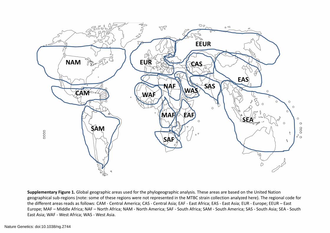
Supplementary Figure 1. Global geographic areas used for the phylogeographic analysis. These areas are based on the United Nation geographical sub‐regions (note: some of these regions were not represented in the MTBC strain collection analyzed here). The regional code for the different areas reads as follows: CAM ‐ Central America; CAS ‐ Central Asia; EAF ‐ East Africa; EAS ‐ East Asia; EUR ‐ Europe; EEUR – East Europe; MAF – Middle Africa; NAF – North Africa; NAM ‐ North America; SAF ‐ South Africa; SAM ‐ South America; SAS ‐ South Asia; SEA ‐ South East Asia; WAF ‐West Africa; WAS ‐West Asia.
Nature Genetics: doi:10.1038/ng.2744
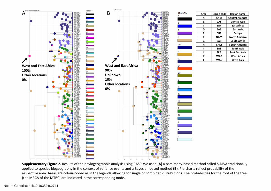
Area Region code Region nameA CAM Central AmericaB CAS Central AsiaC EAF East AfricaD EAS East AsiaE EUR EuropeF NAM North AmericaG SAF South AfricaH SAM South AmericaI SAS South AsiaJ SEA Sout East AsiaK WAF West AfricaL WAS West Asia
Supplementary Figure 2. Results of the phylogeographic analysis using RASP. We used (A) a parsimony‐based method called S‐DIVA traditionally applied to species biogeography in the context of variance events and a Bayesian‐based method (B). Pie‐charts reflect probability of the respective area. Areas are colour‐coded as in the legends allowing for single or combined distributions. The probabilities for the root of the tree (the MRCA of the MTBC) are indicated in the corresponding node.
A B
West and East Africa100%Other locations0%
West and East Africa90%Unknown10%Other locations0%
Nature Genetics: doi:10.1038/ng.2744
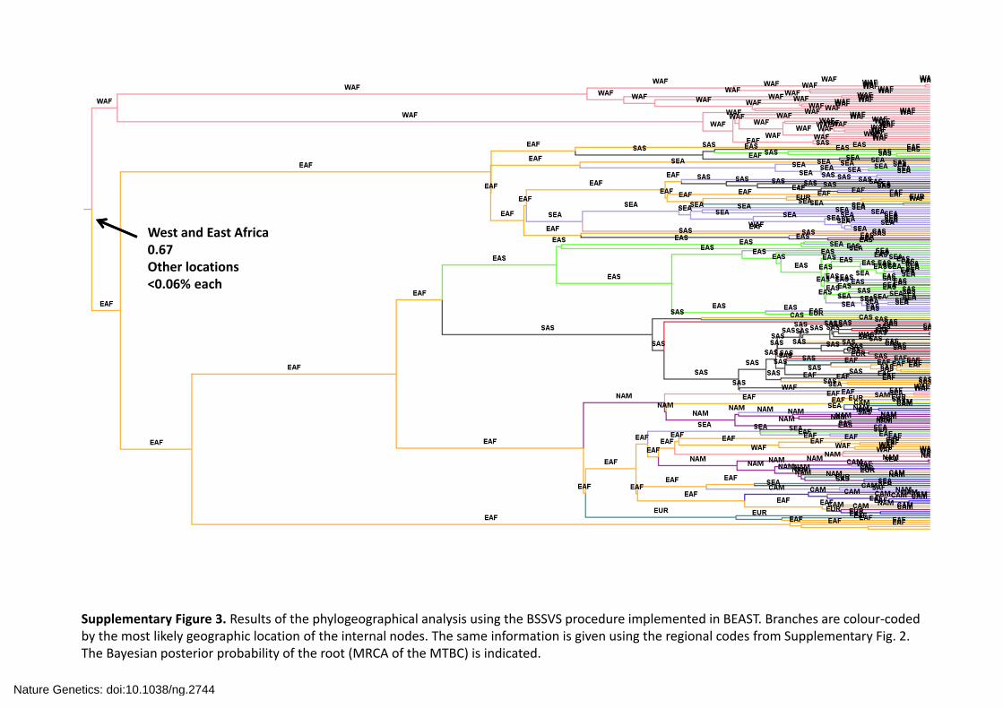
Supplementary Figure 3. Results of the phylogeographical analysis using the BSSVS procedure implemented in BEAST. Branches are colour‐coded by the most likely geographic location of the internal nodes. The same information is given using the regional codes from Supplementary Fig. 2. The Bayesian posterior probability of the root (MRCA of the MTBC) is indicated.
West and East Africa0.67 Other locations<0.06% each
Nature Genetics: doi:10.1038/ng.2744
L3_793601k
L3_282801
L3_858405
L3_SG1
L3_N0197
L3_155808
L3_138007
L3_1016204
L3_N1007
L3_N1024
L2_N0039
L2_N0017
L2_1695
L2_N0005
L2_N0002
L2_N0044_
L2_GT333
L2_T85
L2_N0020
L4_N0107b4
L4_N0011
L4_N0126
L4_N0131
L4_1026403
L4_BTBS-101
L4_N0101
L4_N0163
L4_141702
L4_N0109b4
L4_N0120
L4_N0185
L1_N0065
L1_600603
L1_BTBS-493
L1_N0196
L1_N0132
L1_94701
L1_N1004
L1_N0043
L1_N0062
L1_950545
L1_GT281
L1_1105103
L1_K67
L1_157508
L1_468303
L1_539606
L1_179703
L1_N0182
L6_N0060
L5_1047301
L5_1001003100
100
100100
100
100
100
100
100
100
100
100
100
100
59
100
89
100
4098
77
100
99
100
100
100
100
100
100
100100
100
100
100
100
89
100
100
100
100
100
100100
79100
100
98
59100
200 SNPs
HHHUHL3UMUHBDDEFBFFDAABHHRAHUAAKDMMMEMGMMMDFL3MHMMML3L3L3
NNNNNLNMNNNMMMNNNNMNNNNNNNNNNNNMMMMMMMMMMMNLMNMMMLLL
UzbekistanTurkey
AfghanistanIndiaUK
TanzaniaIran
EritreaNepal
PortugalLaos
South KoreaJapan
IndonesiaCambodiaSingaporeVietnamChina
MongoliaGuatemala
MexicoColombia
USAGermanyEthiopia
NicaraguaIran
GhanaEl SalvadorPuerto Rico
UKChina
Sri LankaEthiopiaSomalia
The PhilippinesAfghanistan
NepalBurma
CambodiaLaos
VietnamThailand
Comoro IslandsTanzaniaSerbia
SingaporeIndia
MalaysiaSenegalGhana
Sierra Leone
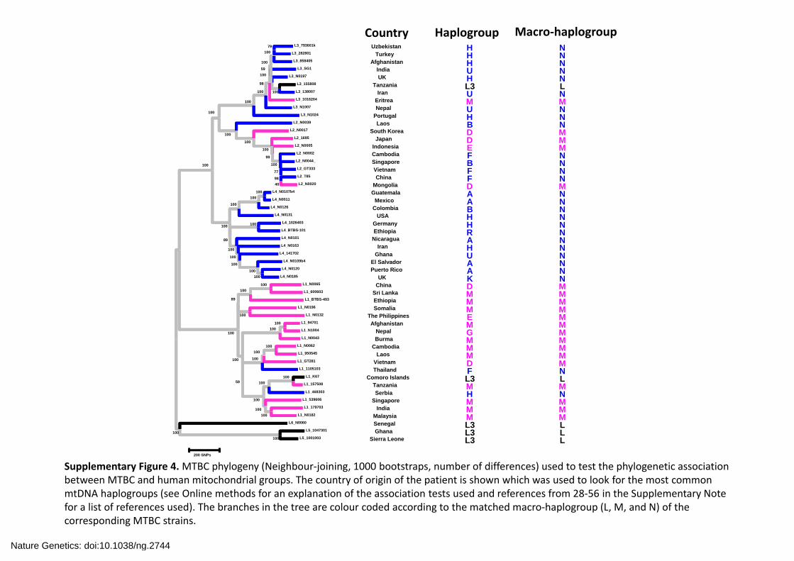
Supplementary Figure 4.MTBC phylogeny (Neighbour‐joining, 1000 bootstraps, number of differences) used to test the phylogenetic association between MTBC and human mitochondrial groups. The country of origin of the patient is shown which was used to look for the most common mtDNA haplogroups (see Online methods for an explanation of the association tests used and references from 28‐56 in the Supplementary Note for a list of references used). The branches in the tree are colour coded according to the matched macro‐haplogroup (L, M, and N) of the corresponding MTBC strains.
Country Haplogroup Macro‐haplogroup
Nature Genetics: doi:10.1038/ng.2744
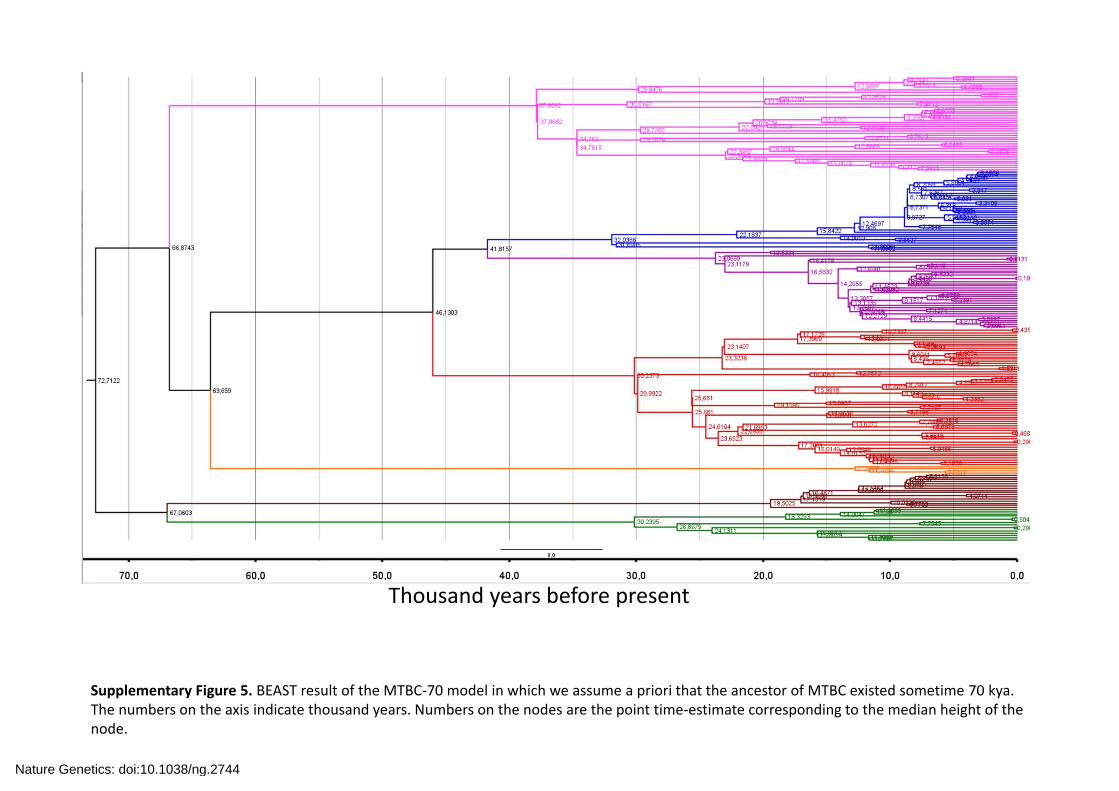
Supplementary Figure 5. BEAST result of the MTBC‐70 model in which we assume a priori that the ancestor of MTBC existed sometime 70 kya. The numbers on the axis indicate thousand years. Numbers on the nodes are the point time‐estimate corresponding to the median height of the node.
Thousand years before present
Nature Genetics: doi:10.1038/ng.2744
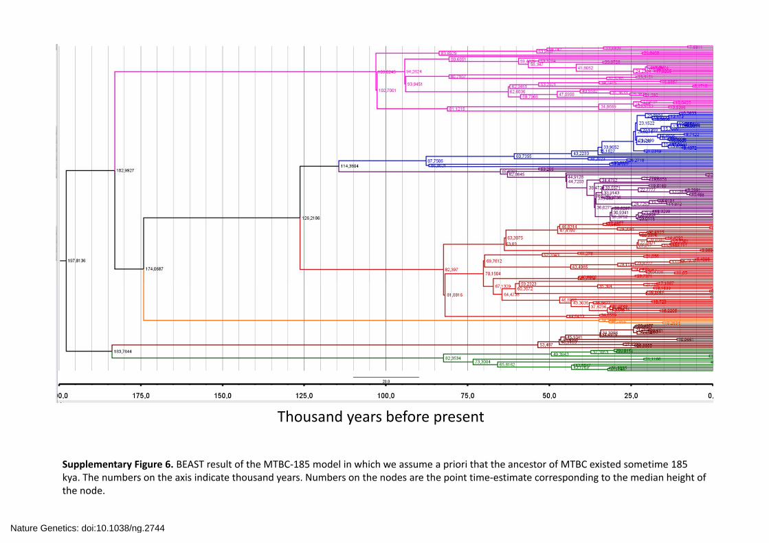
Thousand years before present
Supplementary Figure 6. BEAST result of the MTBC‐185 model in which we assume a priori that the ancestor of MTBC existed sometime 185 kya. The numbers on the axis indicate thousand years. Numbers on the nodes are the point time‐estimate corresponding to the median height of the node.
Nature Genetics: doi:10.1038/ng.2744
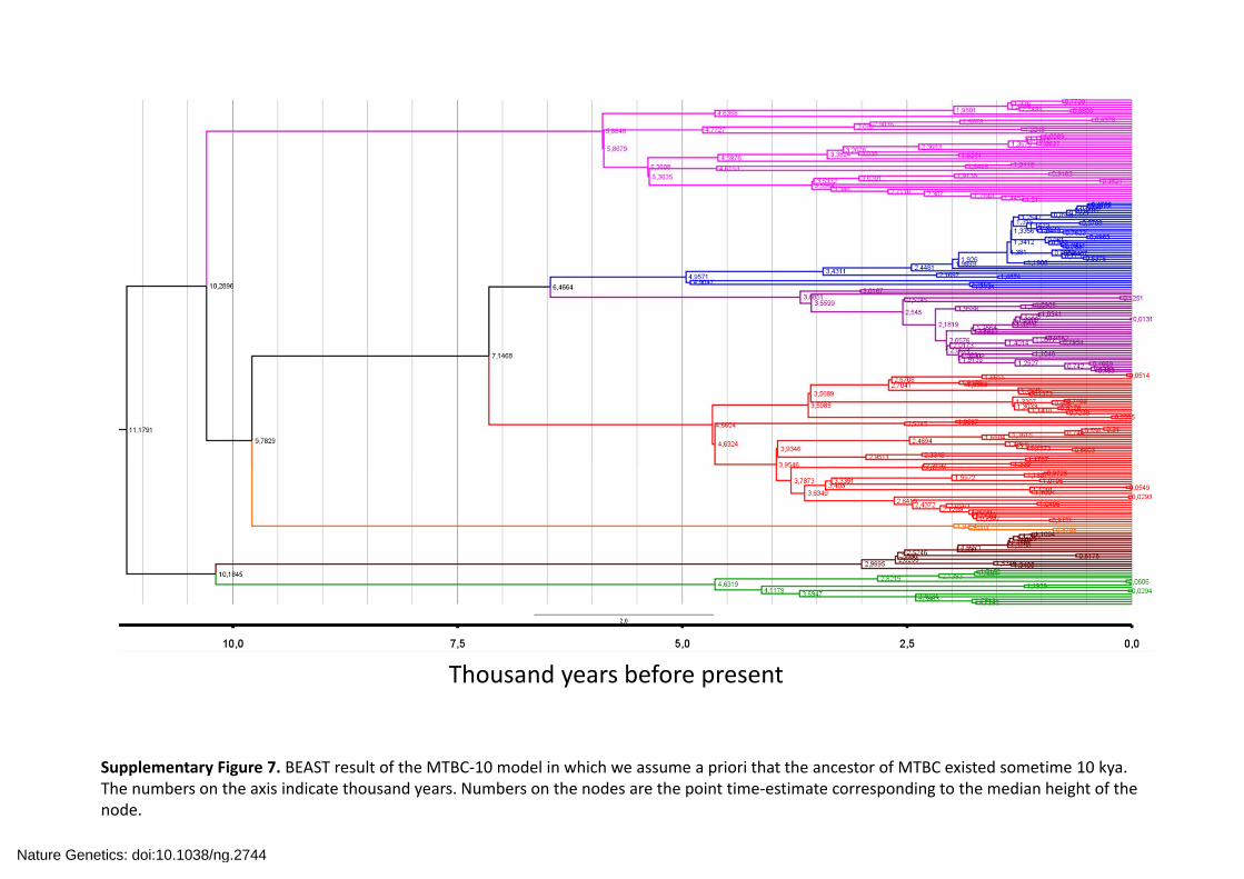
Supplementary Figure 7. BEAST result of the MTBC‐10 model in which we assume a priori that the ancestor of MTBC existed sometime 10 kya. The numbers on the axis indicate thousand years. Numbers on the nodes are the point time‐estimate corresponding to the median height of the node.
Thousand years before present
Nature Genetics: doi:10.1038/ng.2744
0
0.2
0.4
0.6
0.8
1
1.2
1.41‐4
4‐7
7‐10
10‐13
11‐16
16‐19
19‐22
22‐25
25‐28
28‐31
31‐34
34‐37
37‐40
40‐43
43‐46
46‐49
49‐52
52‐55
55‐58
58‐60
Growth ra
te
Time interval in thousand years ago
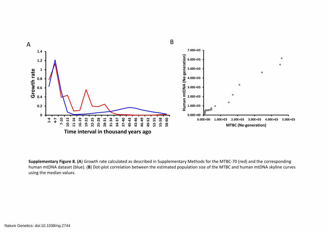
Supplementary Figure 8. (A) Growth rate calculated as described in Supplementary Methods for the MTBC‐70 (red) and the corresponding human mtDNA dataset (blue). (B) Dot‐plot correlation between the estimated population size of the MTBC and human mtDNA skyline curves using the median values.
A B
0.00E+00
1.00E+03
2.00E+03
3.00E+03
4.00E+03
5.00E+03
6.00E+03
7.00E+03
0.00E+00 1.00E+03 2.00E+03 3.00E+03 4.00E+03 5.00E+03
Hum
an m
tDNA (Ne∙gene
ratio
n)
MTBC (Ne∙generation)
Nature Genetics: doi:10.1038/ng.2744
‐0.5
0
0.5
1
1.5
2
2.5
3
3.5
1‐3 3‐5 5‐7 7‐9 9‐11 11‐13 13‐15 15‐17 17‐19 19‐21 21‐23 23‐25 25‐27
Growth ra
te
Time interval in thousand years ago
A B
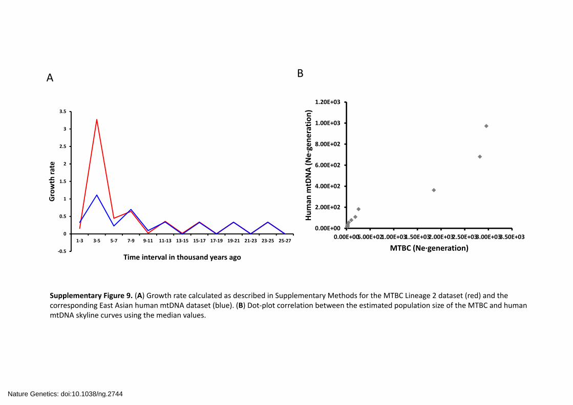
Supplementary Figure 9. (A) Growth rate calculated as described in Supplementary Methods for the MTBC Lineage 2 dataset (red) and the corresponding East Asian human mtDNA dataset (blue). (B) Dot‐plot correlation between the estimated population size of the MTBC and human mtDNA skyline curves using the median values.
0.00E+00
2.00E+02
4.00E+02
6.00E+02
8.00E+02
1.00E+03
1.20E+03
0.00E+005.00E+021.00E+031.50E+032.00E+032.50E+033.00E+033.50E+03
Hum
an m
tDNA (Ne∙gene
ratio
n)
MTBC (Ne∙generation)
Nature Genetics: doi:10.1038/ng.2744
Strain 1 Strain 2 Strain 3
High quality SNPs 1
High quality SNPs 2
High quality SNPs 3
Non‐redundantSNP list
Unfiltered SNPs 1
Unfiltered SNPs 2
Unfiltered SNPs 3
Strain 1 Strain 2 Strain 3
High quality SNPs 1
High quality SNPs 2
High quality SNPs 3
Non‐redundantSNP list
Unfiltered SNPs 1
Unfiltered SNPs 2
Unfiltered SNPs 3
MAQ BWA
MAQSNP ALIGNMENT
BWASNP ALIGNMENT
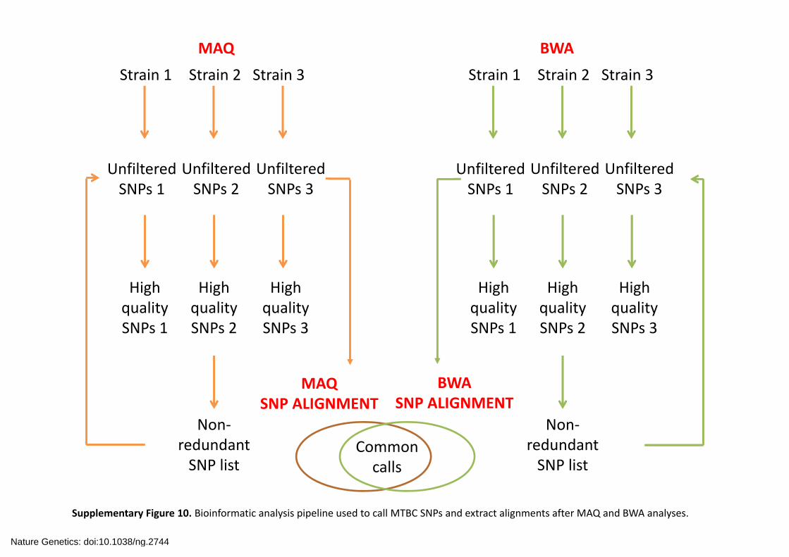
Supplementary Figure 10. Bioinformatic analysis pipeline used to call MTBC SNPs and extract alignments after MAQ and BWA analyses.
Commoncalls
Nature Genetics: doi:10.1038/ng.2744
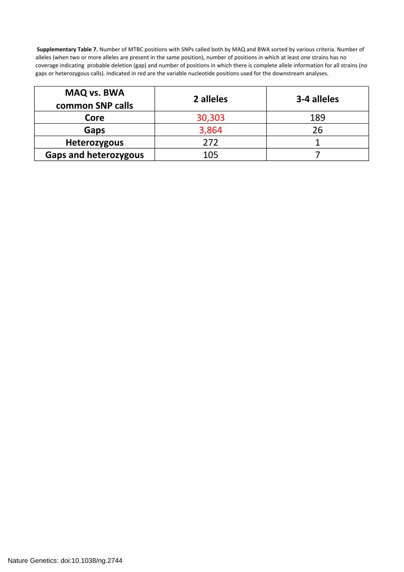
MAQ vs. BWA
common SNP calls2 alleles 3‐4 alleles
Core 30,303 189Gaps 3,864 26
Heterozygous 272 1Gaps and heterozygous 105 7
Supplementary Table 7. Number of MTBC positions with SNPs called both by MAQ and BWA sorted by various criteria. Number of
alleles (when two or more alleles are present in the same position), number of positions in which at least one strains has no
coverage indicating probable deletion (gap) and number of positions in which there is complete allele information for all strains (no
gaps or heterozygous calls). Indicated in red are the variable nucleotide positions used for the downstream analyses.
Nature Genetics: doi:10.1038/ng.2744
Supplementary Note
Ethical statement about the MTBC strains used in this study
The majority of MTBC strains used in this study came from previously established
reference collections1–3. Strains from Nepal and China were collected through ongoing
molecular epidemiological studies. Written informed consent was obtained from all
patients. The studies were ethically approved by the Nepal Health Research Council and
the Ethics Committee of the Canton of Basel (EKBB), Switzerland (Nepalese study),
and by the Ethics Committee of the Shanghai Municipal Centre for Disease Control,
Shanghai, China (Chinese study).
SNP calling after MAQ and BWA mapping
In the case of MAQ, we called the individual SNPs using default settings (minimum
read depth 3, minimum consensus quality 20). In the case of BWA, we called SNPs by
parsing the mapping output with SAMTOOLS4 and keeping those SNPs that were more
likely to be true SNPs (minimum mapping quality 20, maximum read depth 500). In
each case, we generated a non-redundant list of variable positions called with high
confidence in at least one strain and recovered the base call in all other strains as
depicted in Supplementary Figure 10. Once we had the two lists of putative high
confidence calls, we crossed the two lists and kept those calls that fulfilled the following
criteria: 1) they were common to both lists, 2) there were no more than two alleles at
that particular position, 3) they did not involve heterozygous calls, as these are more
likely to represent mapping errors (only positions with deletions were kept), and 4) the
position was not in a repetitive or mobile element. We used ANNOVAR5 and custom
annotation tools to describe each polymorphic position. For a workflow showing the
calling approach used to get the final alignments see Supplementary Figure 10 and
Nature Genetics: doi:10.1038/ng.2744
Supplementary Table 7. The SNPs identified by both mapping approaches are listed in
Supplementary Table 2.
Phylogenetic analyses
Both Maximum-likelihood and Neighbour-joining methods were used to infer the
phylogenetic relationships between the taxa. Maximum-likelihood was implemented in
RAXML6 using GTR as a model of nucleotide substitution and 4 gamma rate categories
correction. The Neighbour-joining method was based on Tamura-Nei distances as
implemented in MEGA 5.07. In both cases, clade support was determined using 1000
bootstrap pseudo-replicates. In both cases, the resulting phylogenies were largely
congruent. In the case of the mitochondrial dataset, the limited phylogenetic information
of the mitochondrial genomes and the presence of some known homoplasies8 led to
some incongruence between the two reconstruction methods. However, coalescent
analyses are not expected to be affected by this as they integrate over all the possible
phylogenies. Given the large number of taxa analyzed, we used FastTree9 to derive the
Maximum-likelihood phylogeny of the human mtDNA dataset. Unlike RAXML,
FastTree does not implement a full Maximum-likelihood approach, but it has been
shown to be more accurate and faster than other Maximum-likelihood approaches when
applied to large datasets.
To identify homoplastic sites, we mapped the SNPs onto the MTBC phylogeny used to
reconstruct the phylogeny and applied the ancestral reconstruction option using
parsimony available in MESQUITE10. The positions that did not fit the phylogeny were
recorded as homoplastic. To delineate different groupings among MTBC strains, we
performed a principal component analysis using STATA s.e.m. version 1011. The three
Nature Genetics: doi:10.1038/ng.2744
first components were introduced in SigmaPlot 12.012 to generate a 3D scatter plot
graph.
Phylogeographic analyses
The Bayesian stochastic search variable selection (BSSVS) implemented in BEAST
was run after defining character states for each taxon, which in this case referred to
geographic locations. The variable stochastic search procedure is also suitable for the
case in which no outgroup is used as in our case13. M. canettii is most closely related to
MTBC but it is a different species influenced by different evolutionary and ecological
processes than MTBC14,15. Moreover, it is almost exclusively associated with East
Africa, which would bias the result of the phylogeographic analyses. The configuration
used for the BEAST runs are explained below.
RASP implements two different methods. A parsimony-based method (S-DIVA)
minimizes the cost of adding new ranges in the ancestral nodes. In this analysis a
maximum of two ancestral areas per node were allowed for range reconstruction. The
second method is a full hierarchical Bayesian approach assuming no prior information
about ancestral distributions; for this analysis ten different chains during 500 thousand
generations were run.
BEAST skyline analyses
A Bayesian skyline model was used to look for changes in the effective population size
per generation in each scenario estimated in 10 different intervals. A skyline plot
measures the changes in population size using the number of coalescent events
estimates at each interval. In all cases, we ran 6-12 chains of 50E6 generations sampled
every 10E3 to assure independent convergence of the chains. Convergence was assessed
using Tracer, ensuring all relevant parameters reached an effective sample size of >100.
Nature Genetics: doi:10.1038/ng.2744
The final skyline for the MTBC-70 scenario was generated by specifying two prior time
points with the aim of reducing uncertainty around the dating and focusing only on the
time of maximum expansion. We defined the height of the complex as 70 kya allowing
+/- 5kya in a normal distribution, and we used 65 +/- 2 kya at the point of split of
MTBC Lineage 1, after corroborating the concordance of both scenarios. To obtain the
skyline plot for Lineage 2 strains, we used the dating of the most recent common
ancestor of the Lineage 2 as derived from the MTBC-70 analysis (32 +/- 5 kya) as the
prior input and ran BEAST using the same parameters as described above. To look at
the correlation between the isolates sampling year and divergence we used Path-O-Gen.
To compare the MTBC and human mtDNA skyline plots and asses their correlation, we
interpolated the values of the curve every one thousand years for MTBC-70 and
mtDNA skyline curves from the median values and calculated the Spearman correlation
coefficient using STATA s.e.m. version 1011. We also calculated for each skyline plot
the growth rate every four thousand years for the global MTBC and mtDNA Neolithic
datasets, and every three thousand years for the East Asia analyses. The growth rate
formula used was as in Gignoux et al.16:
t
tt
tNNr
−
− =0
0)0(
)/ln(
where r refers to the growth rate between time 0 and time t, Nt refers to the median
population size from the skyline plot at time t, N0 refers to the median population size
from the skyline plot at time 0, and t0-t to the time span between both events.
Nature Genetics: doi:10.1038/ng.2744
Correlation between time since most recent common ancestor and predicted
substitution rate in bacteria
For Figure 4 we searched the bibliography for bacterial genome datasets sequenced with
a similar technology, analyzed with BEAST and that are predicted to have a most recent
common ancestor at different age depth21-27. The mean time span since most recent
common ancestor as reported in these different publications was used. Note that for
some of them the age of the group of interest reported in the main text of the
corresponding publication and the time span used in Figure 4 doesn't correlate, this is
because the substitution rate reported many times include an outgroup not just the group
of interest.
1. Hershberg, R. et al. High functional diversity in Mycobacterium tuberculosis driven by genetic drift and human demography. PLoS Biology 6, e311 (2008).
2. Wirth, T. et al. Origin, spread and demography of the Mycobacterium tuberculosis Complex. PLoS Pathogens 4, e1000160 (2008).
3. Gagneux, S. et al. Variable host–pathogen compatibility in Mycobacterium tuberculosis. Proceedings Proc. Natl. Acad. Sci. U.S.A.103, 2869–2873 (2006).
4. Li, H. et al. The Sequence Alignment/Map format and SAMtools. Bioinformatics (Oxford, England) 25, 2078–9 (2009).
5. Wang, K., Li, M. & Hakonarson, H. ANNOVAR: functional annotation of genetic variants from high-‐throughput sequencing data. Nucleic Acids Res. 38, e164–e164 (2010).
6. Stamatakis, A. RAxML-‐VI-‐HPC : maximum likelihood-‐based phylogenetic analyses with thousands of taxa and mixed models. Bioinformatics 22, 2688–2690 (2006).
7. Tamura, K. et al. MEGA5 : Molecular evolutionary genetics analysis using maximum likelihood , evolutionary distance , and maximum parsimony methods research resource. Mol. Biol. and Evol. 28, 2731–2739 (2011).
8. Gonder, M. K. et al. Whole-‐mtDNA genome sequence analysis of ancient African lineages. Mol. Biol. and Evol. 24, 757–68 (2007).
Nature Genetics: doi:10.1038/ng.2744
9. Price, M. N., Dehal, P. S. & Arkin, A. P. FastTree 2 – Approximately maximum-‐likelihood trees for large alignments. PLoS ONE 5, (2010).
10. Maddison, W. P. and D.R. Maddison. 2011. Mesquite: a modular system for evolutionary analysis. Version 2.75 http://mesquiteproject.org.
11. StataCorp. 2007. Stata Statistical Software: Release 10. College Station, TX: StataCorp LP.
12. SigmaPlot 12.0 (Systat Software, Inc., San Jose California USA, www.sigmaplot.com).
13. Lemey, P., Rambaut, A., Drummond, A. J. & Suchard, M. A. Bayesian phylogeography finds its roots. PLoS Comp. Biol. 5, e1000520 (2009).
14. Gutierrez, M. C. et al. Ancient Origin and Gene Mosaicism of the Progenitor of Mycobacterium tuberculosis. PLoS Pathogens 1, e5 (2005).
15. Jang, J. et al. Horizontally acquired genomic islands in the tubercle bacilli. Trends Microbiol. 16, 303-‐308 (2008).
16. Gignoux, C. R., Henn, B. M. & Mountain, J. L. Rapid, global demographic expansions after the origins of agriculture. Proceedings Proc. Natl. Acad. Sci. U.S.A. 108, 6044-‐6049 (2011).
17. Comas, I. et al. Human T cell epitopes of Mycobacterium tuberculosis are evolutionarily hyperconserved. Nat. Genet. 42, 498-‐503 (2010).
18. Casali, N. et al. Microevolution of extensively drug-‐resistant tuberculosis in Russia. Genome Re. 4, 735-‐745 (2012).
19. Comas, I. et al. Whole-‐genome sequencing of rifampicin-‐resistant Mycobacterium tuberculosis strains identifies compensatory mutations in RNA polymerase genes. Nat. Genet. 44, 106-‐110 (2012).
20. Gardy, J. et al. Whole-‐genome sequencing and social-‐network analysis of a tuberculosis outbreak. N. Engl. J. Med. 364, 730-‐739 (2011).
21. Kennemann, L. et al. Helicobacter pylori genome evolution during human infection. Proceedings Proc. Natl. Acad. Sci. U.S.A. 108, 5033-‐5038 (2011).
22. He, M. et al. Emergence and global spread of epidemic healthcare-‐associated Clostridium difficile. Nat. Genet. 45, 1–6 (2012).
23. Holt, K. E. et al. Shigella sonnei genome sequencing and phylogenetic analysis indicate recent global dissemination from Europe. Nat. Genet. 44, 1056-‐1059 (2012).
Nature Genetics: doi:10.1038/ng.2744
24. Mutreja, A. et al. Evidence for several waves of global transmission in the seventh cholera pandemic. Nature 477, 462–465 (2011).
25. Bos, K. I. et al. A draft genome of Yersinia pestis from victims of the Black Death. Nature 478, 506-‐510 (2011).
26. Harris, S. R. et al. Evolution of MRSA During Hospital Transmission and Intercontinental Spread. Science 327, 469–474 (2010).
27. Croucher, N. J. et al. Rapid Pneumococcal Evolution in Response to Clinical Interventions. Science 331, 430–434 (2011).
28. Quintana-‐Murci L. et al. Where west meets east: the complex mtDNA landscape of the southwest and Central Asian corridor. Am J Hum Genet. 74, 827-‐45 (2004).
29. Wang HW. et al. Mitochondrial DNA evidence supports northeast Indian origin of the aboriginal Andamanese in the Late Paleolithic. J Genet Genomics. 38, 117-‐22 (2011).
30. Peng MS. et al. Tracing the Austronesian footprint in Mainland Southeast Asia: a perspective from mitochondrial DNA. Mol Biol Evol. 27, 2417-‐30 (2010).
31. Xue F. et al. A spatial analysis of genetic structure of human populations in China reveals distinct difference between maternal and paternal lineages. Eur J Hum Genet. 16, 705-‐17 (2008).
32. Salas A. et al. Mitochondrial echoes of first settlement and genetic continuity in El Salvador. PLoS One. 4, e6882 (2009).
33. Msaidie S. et al. Genetic diversity on the Comoros Islands shows early seafaring as major determinant of human biocultural evolution in the Western Indian Ocean. Eur J Hum Genet. 19, 89-‐94 (2011).
34. Kivisild T. et al. Ethiopian mitochondrial DNA heritage: tracking gene flow across and around the gate of tears. Am J Hum Genet. 5, 752-‐70 (2004).
35. Tishkoff SA. et al. History of click-‐speaking populations of Africa inferred from mtDNA and Y chromosome genetic variation. Mol Biol Evol. 24, 2180-‐95 (2007).
36. Ottoni C. et al. Mitochondrial analysis of a Byzantine population reveals the differential impact of multiple historical events in South Anatolia. Eur J Hum Genet. 19, 571-‐6 (2011).
37. Fendt L. et al. MtDNA diversity of Ghana: a forensic and phylogeographic view. Forensic Sci Int Genet. 6, 244-‐9(2012).
Nature Genetics: doi:10.1038/ng.2744
38. Hill C. et al. A mitochondrial stratigraphy for island southeast Asia. Am J Hum Genet. 80, 29-‐43 (2007).
39. Asgharzadeh et al. Molecular diversity of mitochondrial DNA in Iranian Azeri ethnicities vis-‐a-‐vis other Azeris in Asia. Iran. J. Biotechnol. 2, 120-‐125 (2011).
40. Tanaka M. et al. Mitochondrial genome variation in eastern Asia and the peopling of Japan. Genome Res. 2004 14, 1832-‐50 (2004).
41. Bodner M. et al. Southeast Asian diversity: first insights into the complex mtDNA structure of Laos. BMC Evol Biol. 11,49 (2011).
42. Green LD, Derr JN, Knight A. mtDNA affinities of the peoples of North-‐Central Mexico. Am J Hum Genet. 66, 989-‐98 (2000).
43. Merriwether DA. et al. mtDNA variation indicates Mongolia may have been the source for the founding population for the New World. Am J Hum Genet. 59, 204-‐12 (1996).
44. Fornarino S. et al. Mitochondrial and Y-‐chromosome diversity of the Tharus (Nepal): a reservoir of genetic variation. BMC Evol Biol. 9,154 (2009).
45. Nuñez C et al. Reconstructing the population history of Nicaragua by means of mtDNA, Y-‐chromosome STRs, and autosomal STR markers. Am J Phys Anthropol. 143, 591-‐600 (2010).
46. Medeiros S. , et al. Haplogroup H Sub-‐Lineages with Mitochondrial SNPs. Forensic Science International: Genetics Supplement Series 1, 285-‐286 (2008).
47. Martínez-‐Cruzado JC. et al. Reconstructing the population history of Puerto Rico by means of mtDNA phylogeographic analysis. Am J Phys Anthropol. 128, 131-‐55 (2005).
48. Rosa A. et al. MtDNA profile of West Africa Guineans: towards a better understanding of the Senegambia region. Ann Hum Genet. 2004 Jul;68(Pt 4):340-‐52. Erratum in: Ann Hum Genet. 2005 Jul;69(Pt 4):499. Ann Hum Genet. 68, 658 (2004).
49. Bosch E. et al. Paternal and maternal lineages in the Balkans show a homogeneous landscape over linguistic barriers, except for the isolated Aromuns. Ann Hum Genet. 70, 459-‐87 (2006).
50. Jackson BA. et al. Mitochondrial DNA genetic diversity among four ethnic groups in Sierra Leone. Am J Phys Anthropol. 128, 156-‐63 (2005).
51. Jin HJ, Tyler-‐Smith C, Kim W. The peopling of Korea revealed by analyses of mitochondrial DNA and Y-‐chromosomal markers. PLoS One. 4, e4210 (2009).
Nature Genetics: doi:10.1038/ng.2744
52. Metspalu M. et al. Most of the extant mtDNA boundaries in south and southwest Asia were likely shaped during the initial settlement of Eurasia by anatomically modern humans. BMC Genet. 5, 26 (2004).
53. Zimmermann B. et al. Forensic and phylogeographic characterization of mtDNA lineages from northern Thailand (Chiang Mai). Int J Legal Med. 123, 495-‐501 (2009).
54. Tabbada KA. et al. Philippine mitochondrial DNA diversity: a populated viaduct between Taiwan and Indonesia? Mol Biol Evol. 27, 21-‐31 (2010).
55. Torroni A. et al. Classification of European mtDNAs from an analysis of three European populations. Genetics. 144, 1835-‐50 (1996).
56. Jin HJ, Tyler-‐Smith C, Kim W. The peopling of Korea revealed by analyses of mitochondrial DNA and Y-‐chromosomal markers. PLoS One. 4, e4210 (2009).
Nature Genetics: doi:10.1038/ng.2744