GSA DATA REPOSITORY 2013294 S.L. Worman et al.

SUPPLEMENTARY INFORMATION

MODEL TABLE DR1. Numeric values of parameterizations used to simulate Tarafaya barchans, listed in order of appearance in text and drawn from Hersen et al. 2004, Andreotti et al. 2002a, 2002b, Elbelrhiti et al. 2005, and field observations by B. Andreotti and P. Claudin (denoted by *)

Parameter Numeric Value α 0.05 Δ 4.65 m

W0 20 m qsat 0.20 m2/day

W∞ (from Eq.4, assuming qf = 0.20qsat)

≈ 30 m ≈ 1.5W0

T = W02/qsat 2000 days

dt, where dt << T 1 day b 45 λc 16.6 m ≈ 0.75W0 σ 0.015 m/day

h0, outside wake zone* 0.05 m, so Wc ≈ 100 m ≈ 5W0 h0, inside wake zone* 0.165 m, so Wc ≈ 60 m ≈ 3W0 h(t)/W0 (aspect ratio) 0.1

RESULTS

Dune Interactions Within a Field

Setting dV/dt = 0 in (4) reveals one unstable equilibrium dune width, W∞,

,              (S1) 

that depends on qf (Hersen et al., 2004). The spatial variation in qf caused by upstream dunes (either persistent dunes or small ones that disappear and become free flux) leads to more than one W∞, potentially permitting divergent behavior of equivalently sized dunes; ‘lucky’ ones, with high qf from upwind, can grow, while others shrink and disappear.

Calving Dynamics

Analytically, recently calved dunes evolve volumetrically according to:

dV 0.5 ∆ ∆ , (S2)

where the first term in (4) has been modified to represent sand supplied to a calf by one horn of its parent. Setting dV/dt = 0 and solving for the parent width that produces stable calves (Wc ≈ 130 m ≈ 6.5W0) implies that parent dunes, as parameterized, cannot support a calf through sand-flux exchange alone.

The first term in (S2) represents the amount of sand leaked to a calf from a parent. After that parent has a subsequent calf, the amount of sand leaked downwind to its earlier calf, is simply the rate at which the calf loses sand, or qsat[Δ+αW0], which is less than the sand influx rate in (S2) and leads to the conclusion that subsequent calves detrimentally disrupt the sand supply of an earlier calf. 

Patch Formation, and Interactions Within Patches

The single dune located at the upwind apex of a patch initiated its formation and subsequently regulates its expansion. Patches begin when a dune stochastically captures enough sand from disappearing upwind dunes to surmount W∞. This pioneer then grows to the calving width, Wc, and ejects calves. However, the sand balance of these progeny is negative (see ‘Calving Dynamics’ above), implying that calf survival is tied to stochastic fluctuations in sand flux in a manner similar to seeded dunes.

Yet, unlike a seeded dune, a calf is mostly sheltered from variations in qf by its parent. Instead of buffering against fluctuations, however, a parent transmits them downwind by calving intermittently. Once a parent calves again, this subsequent calf disrupts the sand supply of the extant calf, increasing its net rate of sand loss. While an upwind calf accentuates the sand-deficit of a down-wind calf, their relative spacing and sizes sometimes allows for their coalescence. This enables some calves to grow downwind of a pioneer horn, slowing their migration and allowing them to capture additional calves. If they become sufficiently sized, they too begin calving and some of their progeny, likewise, go on to form another generation centered on their horns. In this manner, model patches expand laterally and elongate in a stochastic fashion as they travel downwind.

The rate of patch initiation and expansion is controlled by qb,i. As qb,i increases, the probability that seeded dunes are successfully established increases. Conceptually, this is a conditional probability where the rate of dune injection influences the probability, P, that an isolated dune gains an upwind neighbor,

. (S3)

The additional dependence of P on W reveals a positive feedback: If a dune acquires an upwind neighbor, it grows and increases its chances of acquiring another upwind neighbor and growing even further. As a consequence, as qb,i increases more dunes successfully surmount W∞ and proceed to found more rapidly expanding patches.

Megadune Formation

Although dunes producing calves tend to be approximately the same size, and therefore collide infrequently, absorbing smaller dunes can occasionally lead to a positive feedback: An unusually large dune will absorb dunes more and more rapidly as it grows (Figures DR5-DR6). Such very infrequent events interrupt the otherwise homogeneous pattern in the vicinity of the growing ‘megadune’, by starving downwind dunes of sand and creating a vacant, downwind area (Figures DR5-DR6). In nature, unusually large ‘mega dunes’ can occur within a dune field, although the Atmospheric Boundary Layer (Andreotti et al., 2009) ultimately constrains the size of these dunes. Megadune formation in our model, although rare, is likely exaggerated by our conservative formulation of the calving process. In nature, mega-dunes are sufficiently wide that multiple wave trains flank each horn (Elbelrhiti et al., 2008), an effect not included in our model parameterizations. This presumably increases their calving rate and if accounted for would tend to retard such runaway growth (as would interactions with the atmospheric boundary layer, mentioned in the main text).

Unusually large barchans in nature are sometimes assumed to form at the upwind boundary of a dune field, and then are used to back calculate the relative age of the dune field, dividing their distance from the upwind boundary by their propagation velocity. This estimation then provides a rough proxy for the length of time that external conditions have been constant (Hesse, 2009). However, in our model these large dunes form rapidly in place, far downwind of the upwind boundary, suggesting that large-dune migration rates and positions could be misleading indicators of field age. If field-age estimates are systematically too large, this result may have implications for paleo-environmental interpretation, especially for extra-terrestrial settings where other proxies are unavailable.

 

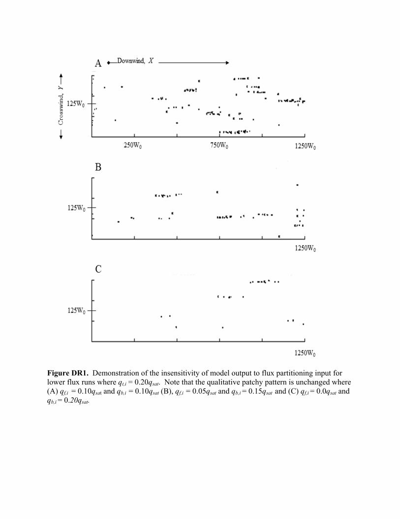
Figure DR1. Demonstration of the insensitivity of model output to flux partitioning input for lower flux runs where qt,i = 0.20qsat. Note that the qualitative patchy pattern is unchanged where (A) qf,i = 0.10qsat and qb,i = 0.10qsat (B), qf,i = 0.05qsat and qb,i = 0.15qsat and (C) qf,i = 0.0qsat and qb,i = 0.20qsat.

 

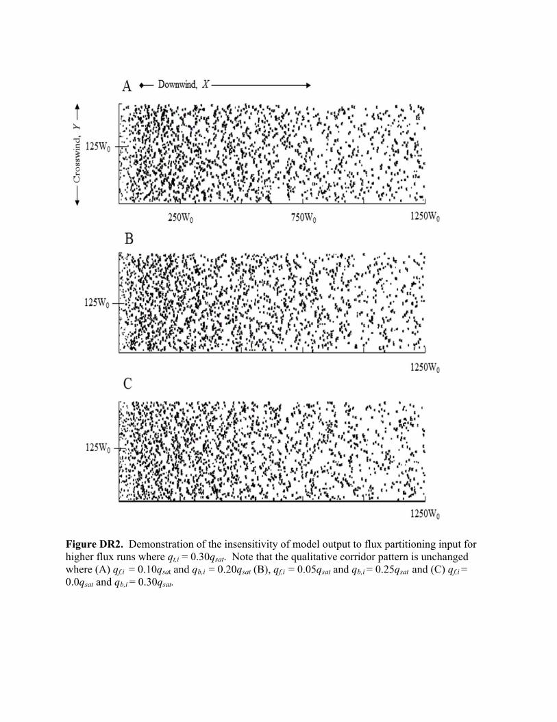
Figure DR2. Demonstration of the insensitivity of model output to flux partitioning input for higher flux runs where qt,i = 0.30qsat. Note that the qualitative corridor pattern is unchanged where (A) qf,i = 0.10qsat and qb,i = 0.20qsat (B), qf,i = 0.05qsat and qb,i = 0.25qsat and (C) qf,i = 0.0qsat and qb,i = 0.30qsat.

 

 

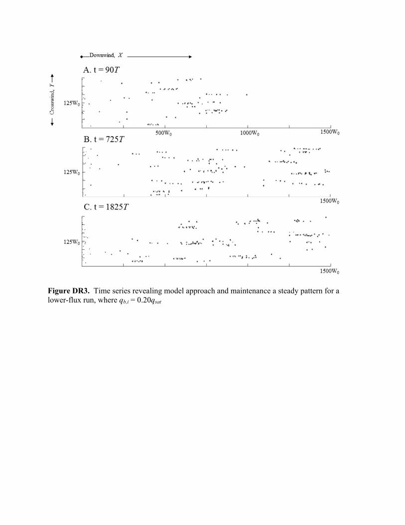
Figure DR3. Time series revealing model approach and maintenance a steady pattern for a lower-flux run, where qb,i = 0.20qsat

 

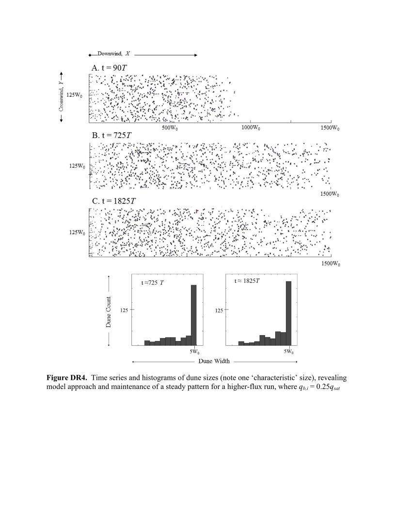
Figure DR4. Time series and histograms of dune sizes (note one ‘characteristic’ size), revealing model approach and maintenance of a steady pattern for a higher-flux run, where qb,i = 0.25qsat

 

 

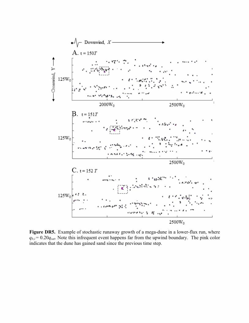
Figure DR5. Example of stochastic runaway growth of a mega-dune in a lower-flux run, where qb,i = 0.20qsat. Note this infrequent event happens far from the upwind boundary. The pink color indicates that the dune has gained sand since the previous time step.  

 

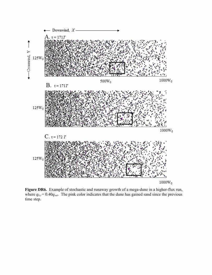
Figure DR6. Example of stochastic and runaway growth of a mega-dune in a higher-flux run, where qb,i = 0.40qsat. The pink color indicates that the dune has gained sand since the previous time step.  

 

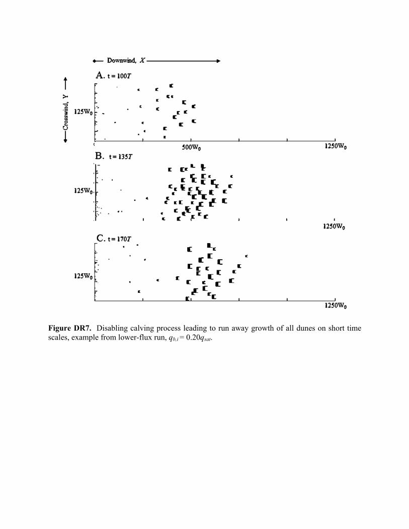
Figure DR7. Disabling calving process leading to run away growth of all dunes on short time scales, example from lower-flux run, qb,i = 0.20qsat.

 

   

 

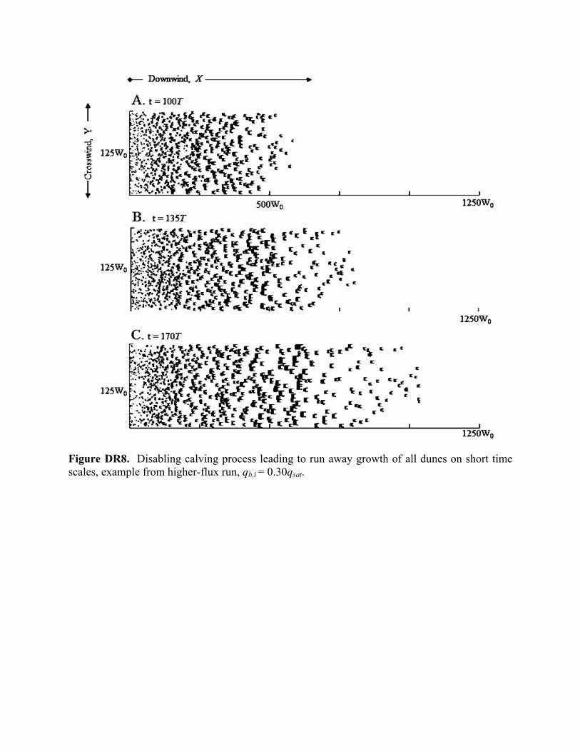
Figure DR8. Disabling calving process leading to run away growth of all dunes on short time scales, example from higher-flux run, qb,i = 0.30qsat.

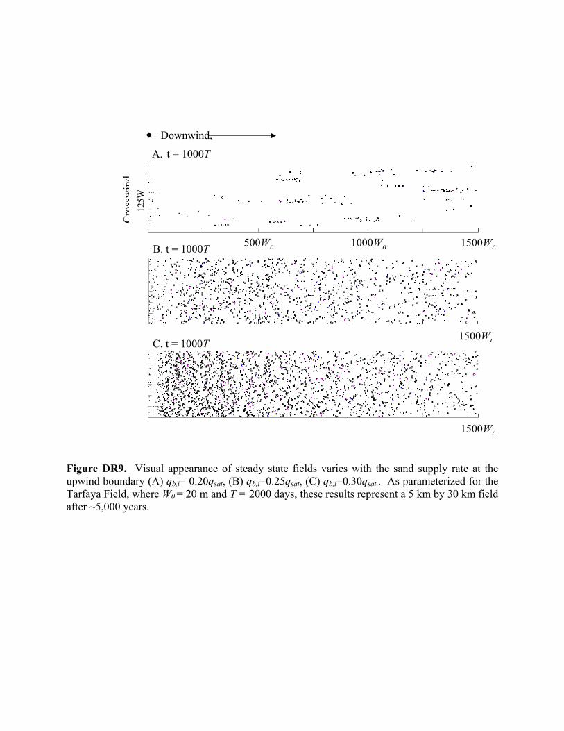
Figure DR9. Visual appearance of steady state fields varies with the sand supply rate at the upwind boundary (A) qb,i= 0.20qsat, (B) qb,i=0.25qsat, (C) qb,i=0.30qsat.. As parameterized for the Tarfaya Field, where W0 = 20 m and T = 2000 days, these results represent a 5 km by 30 km field after ~5,000 years.

   

125W

0

250W

0

Cro

ssw

ind

t = 900

t = 900

 

 

Downwind,

 

125W

 

A. t = 1000T

B. t = 1000T

C. t = 1000T 1500W

0

1500W0

1500W0 1000W

0 500W

0

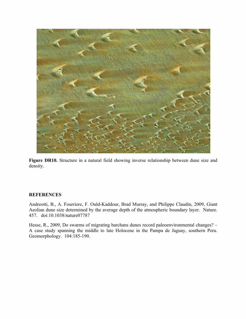
Figure DR10. Structure in a natural field showing inverse relationship between dune size and density.

REFERENCES

Andreotti, B., A. Fourriere, F. Ould-Kaddour, Brad Murray, and Philippe Claudin, 2009, Giant Aeolian dune size determined by the average depth of the atmospheric boundary layer. Nature. 457. doi:10.1038/nature07787 

Hesse, R., 2009, Do swarms of migrating barchans dunes record paleoenvironmental changes? – A case study spanning the middle to late Holocene in the Pampa de Jaguay, southern Peru. Geomorphology. 104:185-190.