Embed Size (px)
Citation preview
www.sciencemag.org/cgi/content/full/science.aav0652/DC1
Supplementary Materials for Magnetic hysteresis up to 80 kelvin in a dysprosium metallocene
single-molecule magnet
Fu-Sheng Guo, Benjamin M. Day, Yan-Cong Chen, Ming-Liang Tong, Akseli Mansikkamäki, Richard A. Layfield*
*Corresponding author. Email: [email protected]
Published 18 October 2018 on Science First ReleaseDOI: 10.1126/science.aav0652
This PDF file includes:
Materials and Methods Figs. S1 to S51 Tables S1 to S18 Captions for Movies S1 to S7 Captions for Data S1 to S3 References
Other Supporting Online Material for this manuscript includes the following: (available at www.sciencemag.org/cgi/content/full/science.aav0652/DC1)
Movies S1 to S7 Data S1 to S3
Data S1: optimized geometry (xyz file) Data S2: displacements (xyz file) Data S3: magnetism data (Excel file)
Materials and Methods
General Procedures All reactions were carried out under rigorous anaerobic, anhydrous conditions under argon or nitrogen atmospheres using standard Schlenk line and glovebox techniques. All solvents were refluxed over an appropriate drying agent for a minimum of three days (molten potassium for toluene and benzene, Na/K alloy for hexane, CaH2 for CH2Cl2) before distilling, and were stored in ampoules over activated 4 Å molecular sieves (toluene, hexane, benzene, CH2Cl2). NaCpiPr5 (37), Dy(BH4)3(THF)3 (38), KCp* (39) and [Et3Si(H)SiEt3][B(C6F5)4] (15) were prepared according to literature procedures. Elemental analyses were carried out at London Metropolitan University, U.K. IR spectra were collected on a Bruker Alpha FTIR spectrometer fitted with a Platinum ATR module. Synthesis of [CpiPr5Dy(BH4)2THF] (1): Toluene (15 ml) was added to an ampoule containing a mixture of NaCpiPr5 (895 mg, 3.0 mmol), Dy(BH4)3(THF)3 (1328 mg, 3.0 mmol) and a glass coated stirrer bar, and the resulting suspension was stirred at room temperature overnight. The toluene was removed under vacuum and the product was extracted into hexane (3 × 10 mL) and filtered. The filtrate was concentrated in vacuo until incipient crystallisation occurred. The solution was then gently warmed to re-dissolve the microcrystalline solid and the solution was stored at –40°C overnight, yielding pale yellow crystals of 1. Yield = 1166 mg, 72 %. Elemental analysis found (calcd.) % for C24H51B2ODy: C 52.13 (53.40); H 9.67 (9.52). IR spectra (cm−1): 2973s, 2929s, 2871s, 2462s, 2364w, 2309m, 2262w, 2198m, 2131s, 1458s, 1365s, 1320w, 1252m, 1194s, 1175s, 1098s, 1083s, 1041m, 1004s, 957w, 909m, 856s, 749w, 666m, 545m, 525s, 484s, 454s. Synthesis of [CpiPr5DyCp*(BH4)] (2): Toluene (15 ml) was added to an ampoule containing a mixture of 1 (532 mg, 1.0 mmol), KCp* (174 mg, 1.0 mmol) and a glass coated stirrer bar, and the resulting suspension was stirred at 110°C for two days. The toluene was removed under vacuum and the product was extracted into hexane (3 × 10 mL) and filtered. After removal of the solvent, a yellow powder was obtained and recrystallized from hexane at –40 °C to yield yellow crystals of 2. Yield = 190 mg, 32 %. Elemental analysis found (calcd.) % for C30H54BDy: C 61.03(61.27); H 9.39 (9.26). IR spectra (cm−1): 2966s, 2908s, 2866s, 2441m, 2398m, 2294w, 2248w, 2133m, 2038w, 1998w, 1446m, 1380s, 1366s, 1295w, 1218w, 1197w, 1158m, 1129s, 1090m, 1058w, 1030w, 955w, 906w, 861w, 803w, 768w, 710w, 595w, 542w, 504s, 452w. Synthesis of [CpiPr5DyCp*][B(C6F5)4] (3): Cold (–40 °C) hexane (10 ml) was added into a cold ampoule containing [Et3Si(H)SiEt3][B(C6F5)4] (180 mg, 0.20 mmol) and a glass coated stirrer bar. Then, a cold (–40 °C) hexane (10 ml) solution of [CpiPr5DyCp*(BH4)] (118 mg, 0.2 mmol) was slowly added to the ampoule, then the resulting suspension was sonicated for three minutes and stirred overnight to give a yellow solid. After letting the solid settle, as much of the solution as possible was decanted away and hexane (10 ml) was added. This was repeated five times before removal of residual volatiles in vacuo gave a yellow solid. A crystalline sample of 3 was obtained by storing a saturated dichloromethane solution at –40°C overnight. Isolated crystalline yield = 150 mg, 60 %. Elemental analysis found (calcd.)% for C54H50BDyF20: C: 51.63 (51.79); H 4.11 (4.02). IR spectra (cm−1): 2990w, 2970w, 2875w, 2792w, 1641m, 1512s, 1458s, 1424m, 1384m, 1371m, 1310w, 1277m, 1159w, 1084s, 1031w, 978s, 904w, 799w, 775s, 756s, 726w, 684s, 660s, 610w, 573m, 506m, 476w.
2
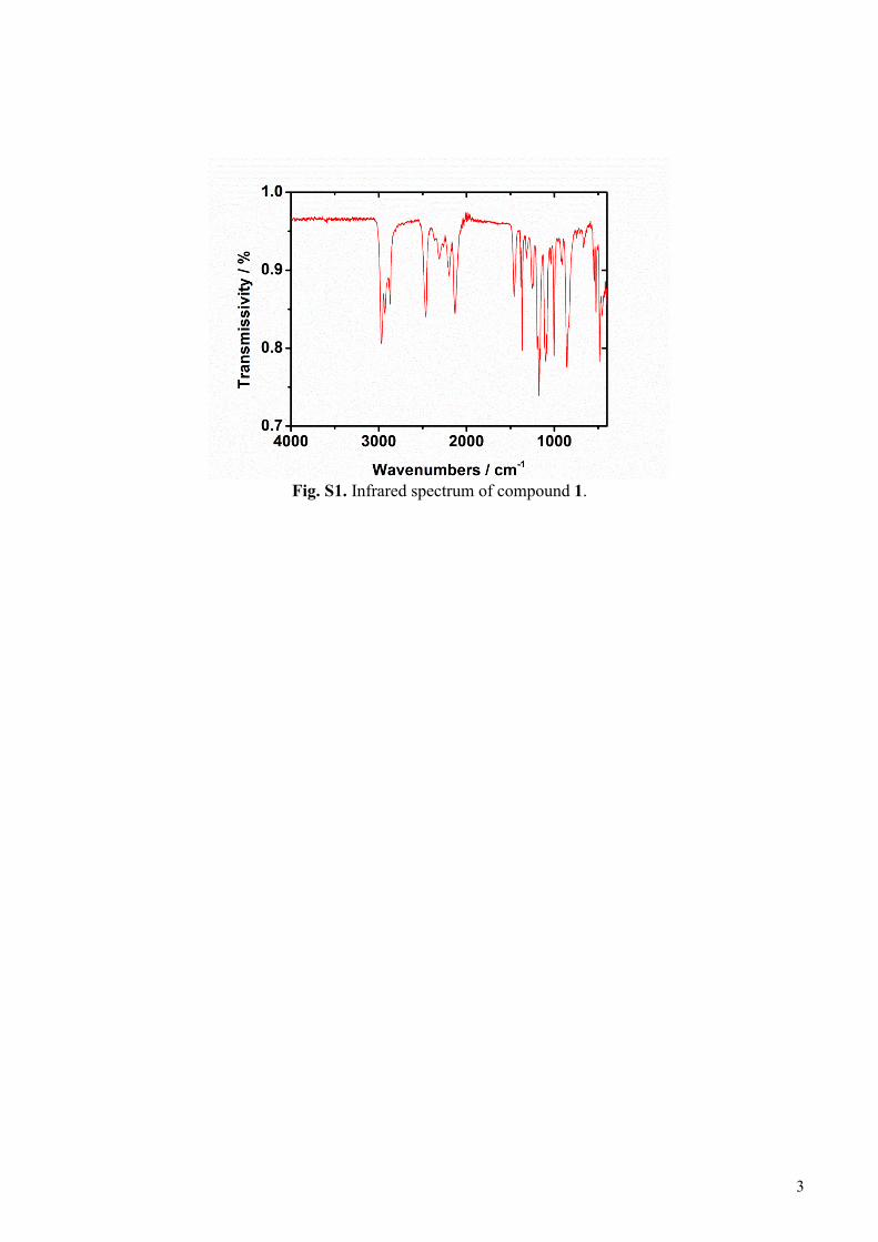
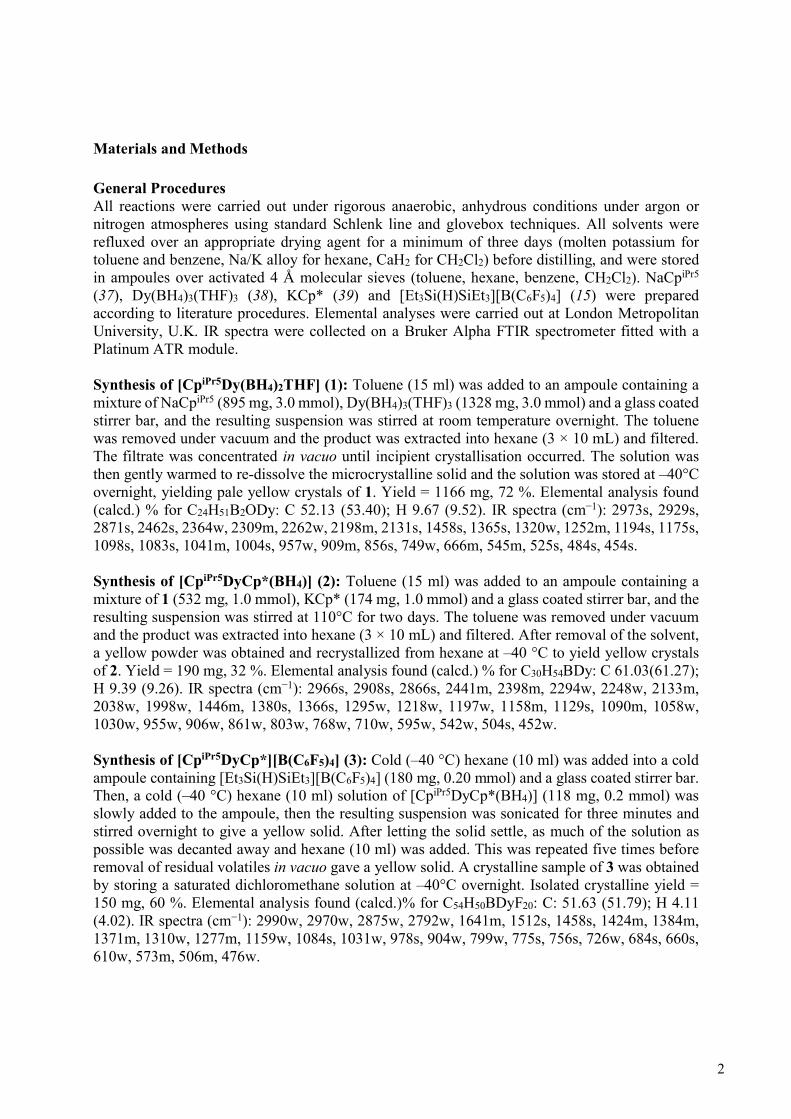
Fig. S1. Infrared spectrum of compound 1.
3
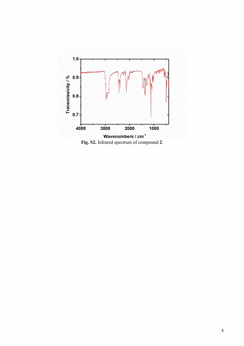
Fig. S2. Infrared spectrum of compound 2.
4
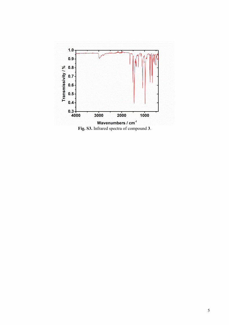
Fig. S3. Infrared spectra of compound 3.
5
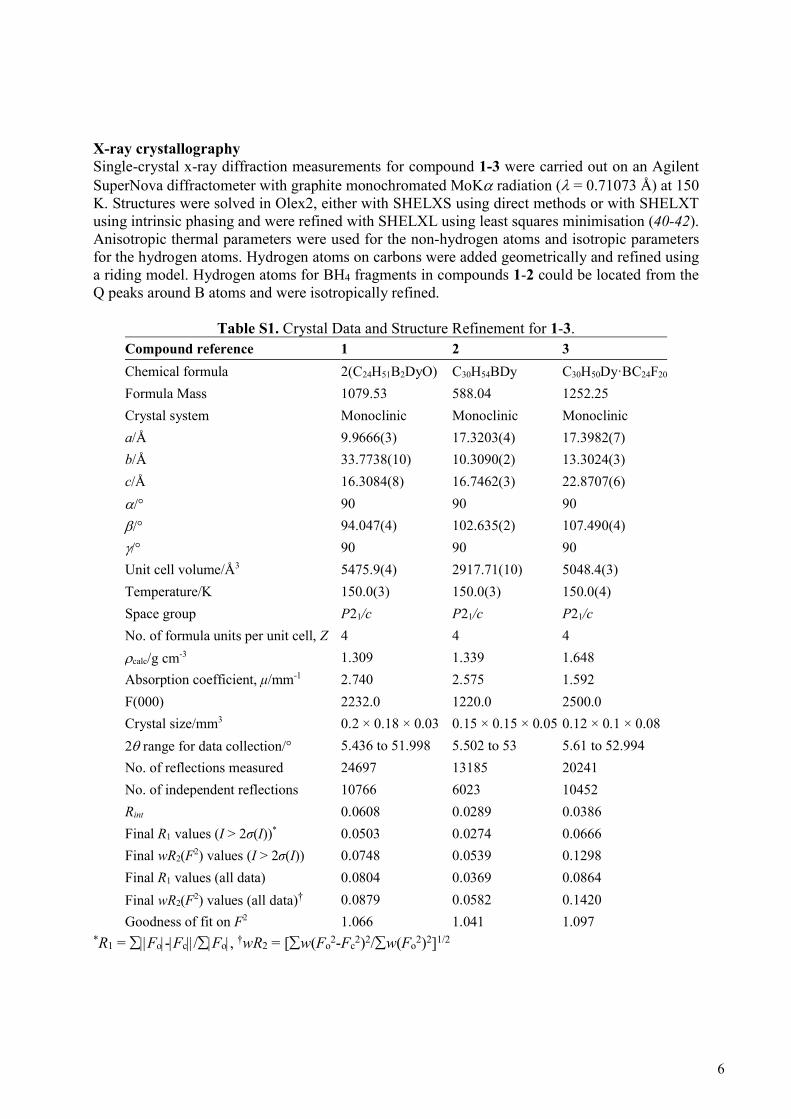
X-ray crystallography Single-crystal x-ray diffraction measurements for compound 1-3 were carried out on an Agilent SuperNova diffractometer with graphite monochromated MoK radiation ( = 0.71073 Å) at 150 K. Structures were solved in Olex2, either with SHELXS using direct methods or with SHELXT using intrinsic phasing and were refined with SHELXL using least squares minimisation (40-42). Anisotropic thermal parameters were used for the non-hydrogen atoms and isotropic parameters for the hydrogen atoms. Hydrogen atoms on carbons were added geometrically and refined using a riding model. Hydrogen atoms for BH4 fragments in compounds 1-2 could be located from the Q peaks around B atoms and were isotropically refined.
Table S1. Crystal Data and Structure Refinement for 1-3.
Compound reference 1 2 3
Chemical formula 2(C24H51B2DyO) C30H54BDy C30H50Dy·BC24F20
Formula Mass 1079.53 588.04 1252.25
Crystal system Monoclinic Monoclinic Monoclinic
a/Å 9.9666(3) 17.3203(4) 17.3982(7)
b/Å 33.7738(10) 10.3090(2) 13.3024(3)
c/Å 16.3084(8) 16.7462(3) 22.8707(6)
/° 90 90 90
/° 94.047(4) 102.635(2) 107.490(4)
/° 90 90 90
Unit cell volume/Å3 5475.9(4) 2917.71(10) 5048.4(3)
Temperature/K 150.0(3) 150.0(3) 150.0(4)
Space group P21/c P21/c P21/c
No. of formula units per unit cell, Z 4 4 4
calc/g cm-3 1.309 1.339 1.648
Absorption coefficient, μ/mm-1 2.740 2.575 1.592
F(000) 2232.0 1220.0 2500.0
Crystal size/mm3 0.2 × 0.18 × 0.03 0.15 × 0.15 × 0.05 0.12 × 0.1 × 0.08
2 range for data collection/° 5.436 to 51.998 5.502 to 53 5.61 to 52.994
No. of reflections measured 24697 13185 20241
No. of independent reflections 10766 6023 10452
Rint 0.0608 0.0289 0.0386
Final R1 values (I > 2σ(I))* 0.0503 0.0274 0.0666
Final wR2(F2) values (I > 2σ(I)) 0.0748 0.0539 0.1298
Final R1 values (all data) 0.0804 0.0369 0.0864
Final wR2(F2) values (all data)† 0.0879 0.0582 0.1420
Goodness of fit on F2 1.066 1.041 1.097 *R1 = Fo-Fc/Fo, †wR2 = [w(Fo
2-Fc2)2/w(Fo
2)2]1/2
6
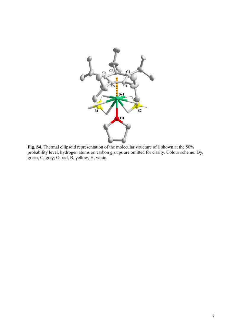
Fig. S4. Thermal ellipsoid representation of the molecular structure of 1 shown at the 50% probability level, hydrogen atoms on carbon groups are omitted for clarity. Colour scheme: Dy, green; C, grey; O, red; B, yellow; H, white.
7
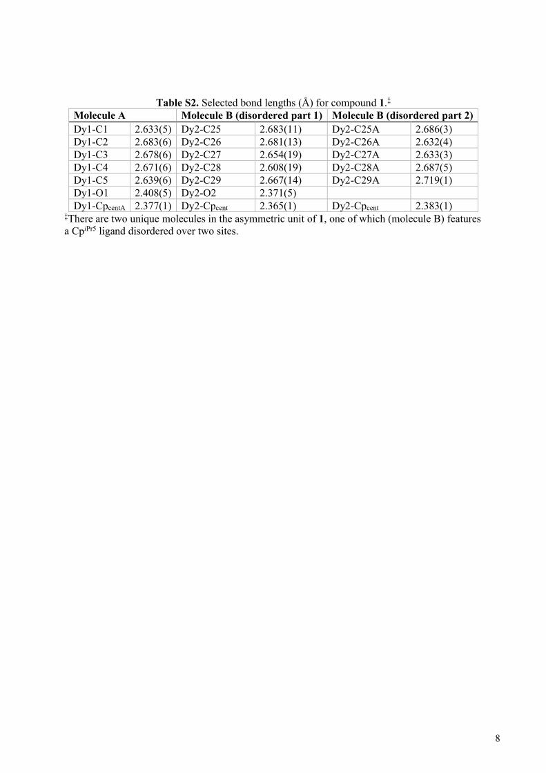
Table S2. Selected bond lengths (Å) for compound 1.‡ Molecule A Molecule B (disordered part 1) Molecule B (disordered part 2)
Dy1-C1 2.633(5) Dy2-C25 2.683(11) Dy2-C25A 2.686(3) Dy1-C2 2.683(6) Dy2-C26 2.681(13) Dy2-C26A 2.632(4) Dy1-C3 2.678(6) Dy2-C27 2.654(19) Dy2-C27A 2.633(3) Dy1-C4 2.671(6) Dy2-C28 2.608(19) Dy2-C28A 2.687(5) Dy1-C5 2.639(6) Dy2-C29 2.667(14) Dy2-C29A 2.719(1) Dy1-O1 2.408(5) Dy2-O2 2.371(5) Dy1-CpcentA 2.377(1) Dy2-Cpcent 2.365(1) Dy2-Cpcent 2.383(1)
‡There are two unique molecules in the asymmetric unit of 1, one of which (molecule B) features a CpiPr5 ligand disordered over two sites.
8
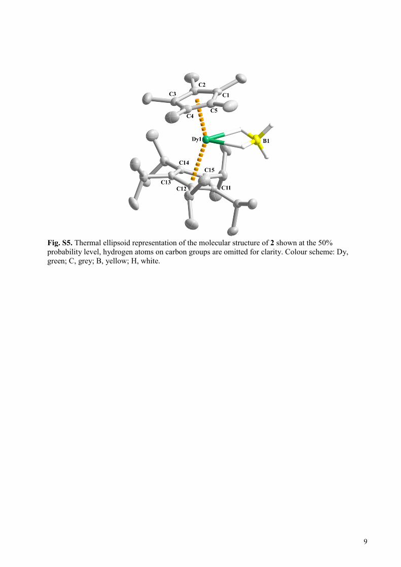
Fig. S5. Thermal ellipsoid representation of the molecular structure of 2 shown at the 50% probability level, hydrogen atoms on carbon groups are omitted for clarity. Colour scheme: Dy, green; C, grey; B, yellow; H, white.
9
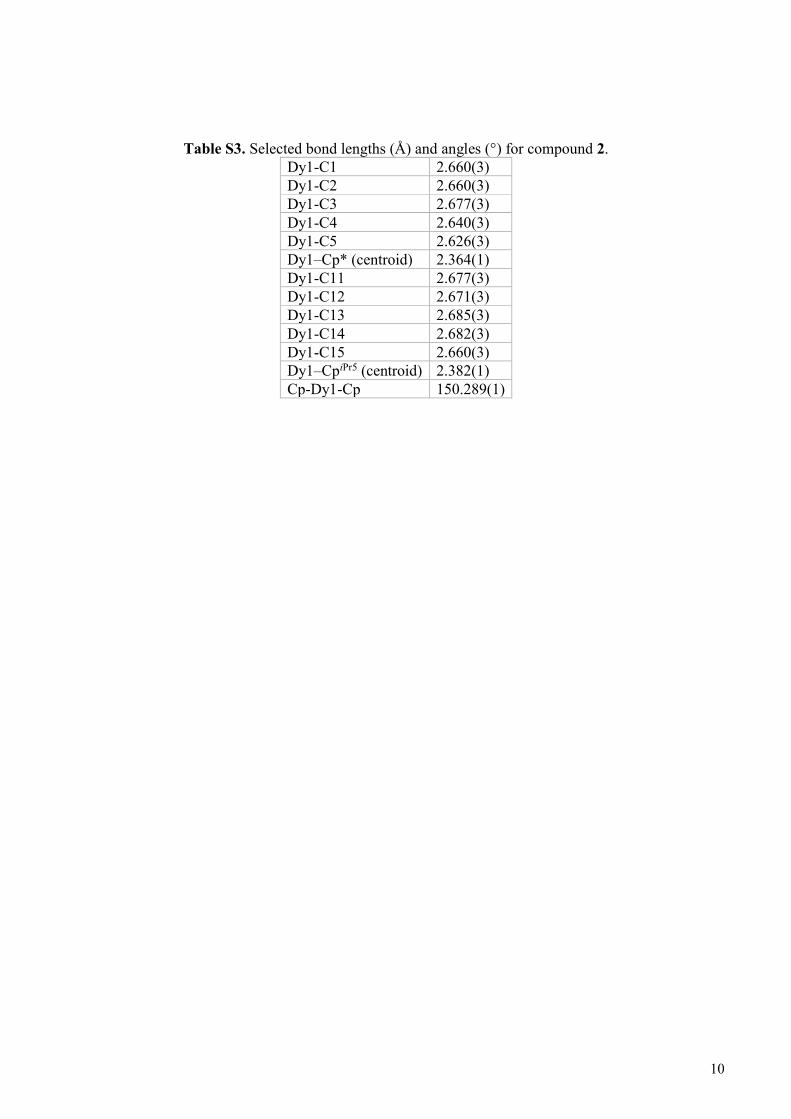
Table S3. Selected bond lengths (Å) and angles (°) for compound 2. Dy1-C1 2.660(3) Dy1-C2 2.660(3) Dy1-C3 2.677(3) Dy1-C4 2.640(3) Dy1-C5 2.626(3) Dy1–Cp* (centroid) 2.364(1) Dy1-C11 2.677(3) Dy1-C12 2.671(3) Dy1-C13 2.685(3) Dy1-C14 2.682(3) Dy1-C15 2.660(3) Dy1–CpiPr5 (centroid) 2.382(1) Cp-Dy1-Cp 150.289(1)
10
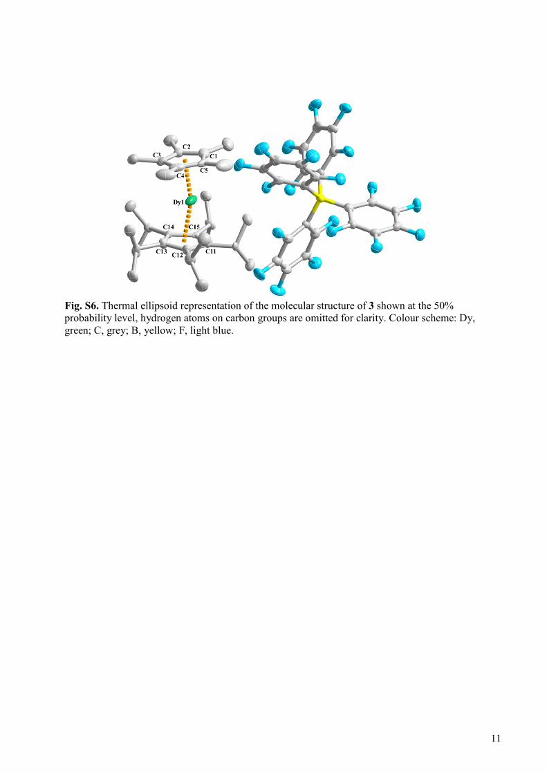
Fig. S6. Thermal ellipsoid representation of the molecular structure of 3 shown at the 50% probability level, hydrogen atoms on carbon groups are omitted for clarity. Colour scheme: Dy, green; C, grey; B, yellow; F, light blue.
11
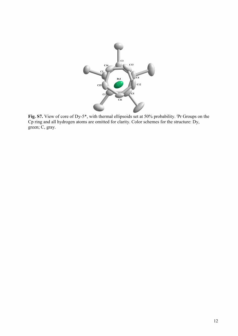
Fig. S7. View of core of Dy-5*, with thermal ellipsoids set at 50% probability. iPr Groups on the Cp ring and all hydrogen atoms are omitted for clarity. Color schemes for the structure: Dy, green; C, gray.
12
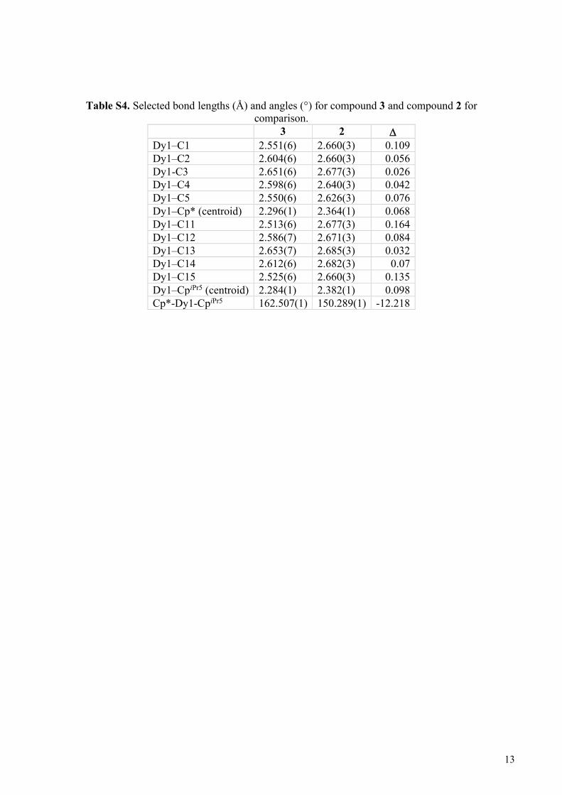
Table S4. Selected bond lengths (Å) and angles (°) for compound 3 and compound 2 for comparison.
3 2 Dy1–C1 2.551(6) 2.660(3) 0.109 Dy1–C2 2.604(6) 2.660(3) 0.056 Dy1-C3 2.651(6) 2.677(3) 0.026 Dy1–C4 2.598(6) 2.640(3) 0.042 Dy1–C5 2.550(6) 2.626(3) 0.076 Dy1–Cp* (centroid) 2.296(1) 2.364(1) 0.068 Dy1–C11 2.513(6) 2.677(3) 0.164 Dy1–C12 2.586(7) 2.671(3) 0.084 Dy1–C13 2.653(7) 2.685(3) 0.032 Dy1–C14 2.612(6) 2.682(3) 0.07 Dy1–C15 2.525(6) 2.660(3) 0.135 Dy1–CpiPr5 (centroid) 2.284(1) 2.382(1) 0.098 Cp*-Dy1-CpiPr5 162.507(1) 150.289(1) -12.218
13
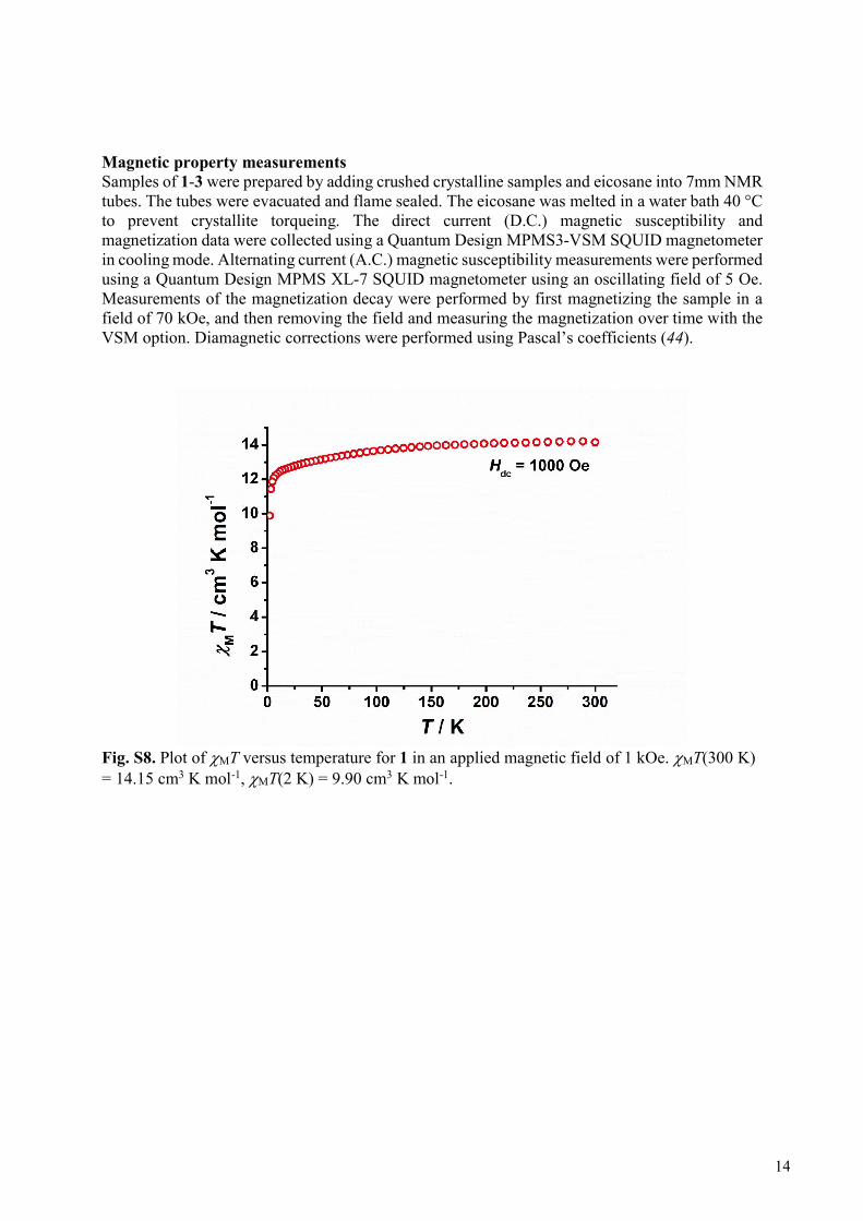
Magnetic property measurements Samples of 1-3 were prepared by adding crushed crystalline samples and eicosane into 7mm NMR tubes. The tubes were evacuated and flame sealed. The eicosane was melted in a water bath 40 °C to prevent crystallite torqueing. The direct current (D.C.) magnetic susceptibility and magnetization data were collected using a Quantum Design MPMS3-VSM SQUID magnetometer in cooling mode. Alternating current (A.C.) magnetic susceptibility measurements were performed using a Quantum Design MPMS XL-7 SQUID magnetometer using an oscillating field of 5 Oe. Measurements of the magnetization decay were performed by first magnetizing the sample in a field of 70 kOe, and then removing the field and measuring the magnetization over time with the VSM option. Diamagnetic corrections were performed using Pascal’s coefficients (44).
Fig. S8. Plot of MT versus temperature for 1 in an applied magnetic field of 1 kOe. MT(300 K) = 14.15 cm3 K mol-1, MT(2 K) = 9.90 cm3 K mol-1.
14
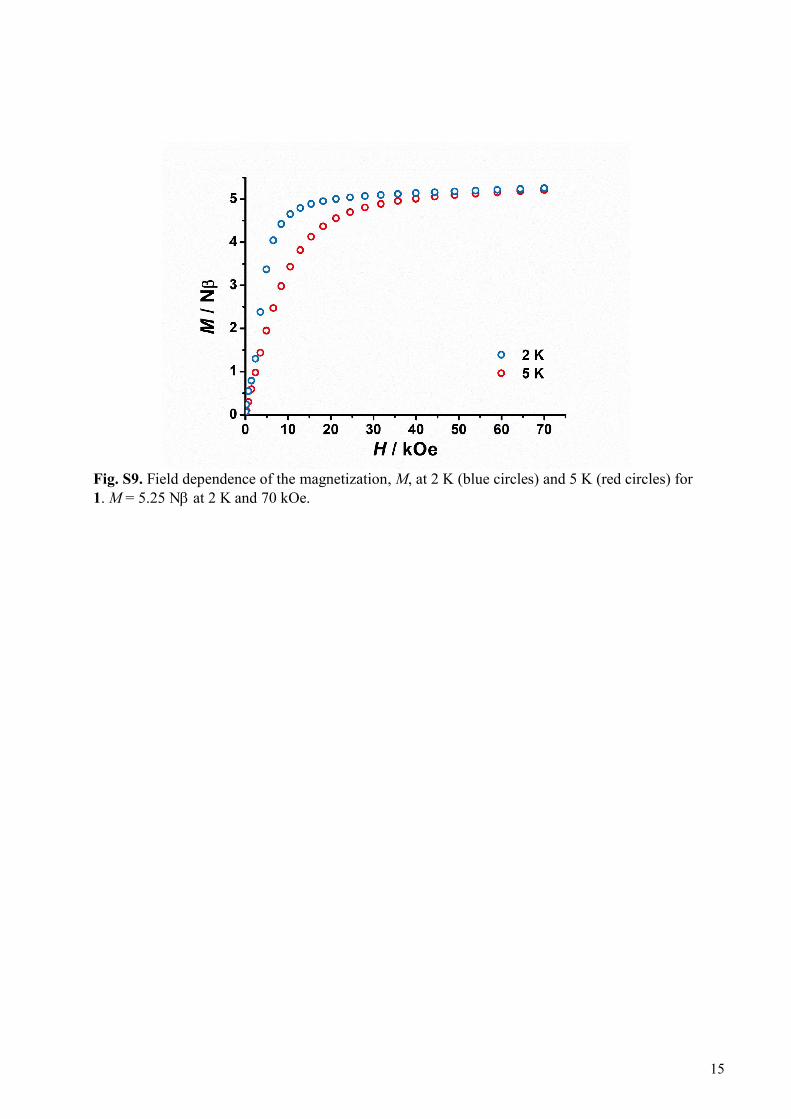
Fig. S9. Field dependence of the magnetization, M, at 2 K (blue circles) and 5 K (red circles) for 1. M = 5.25 N at 2 K and 70 kOe.
15
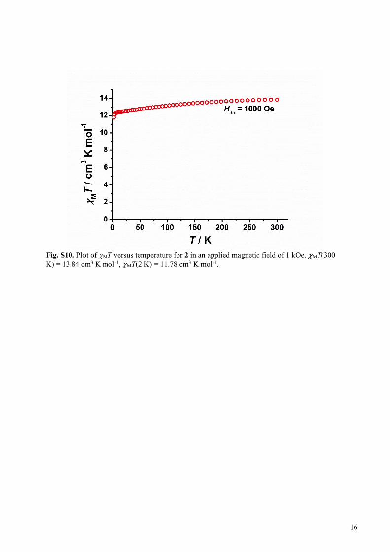
Fig. S10. Plot of MT versus temperature for 2 in an applied magnetic field of 1 kOe. MT(300 K) = 13.84 cm3 K mol-1, MT(2 K) = 11.78 cm3 K mol-1.
16
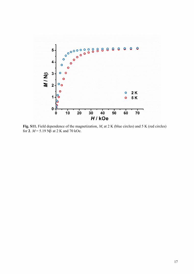
Fig. S11. Field dependence of the magnetization, M, at 2 K (blue circles) and 5 K (red circles) for 2. M = 5.19 N at 2 K and 70 kOe.
17
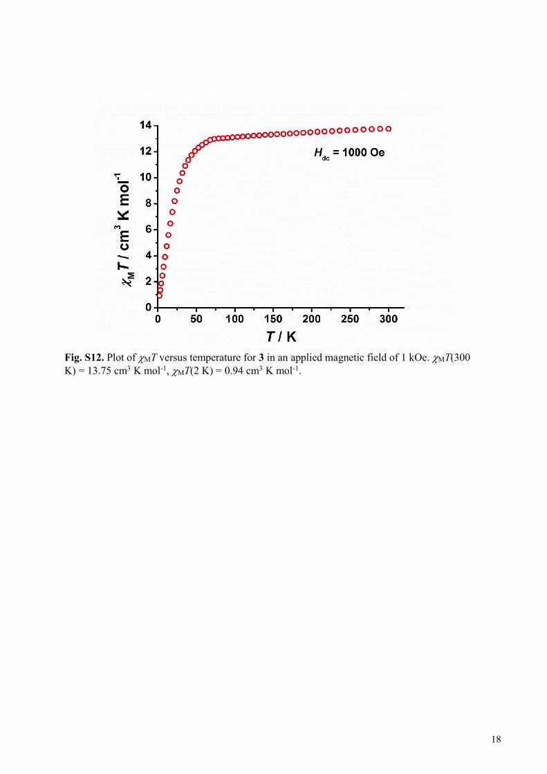
Fig. S12. Plot of MT versus temperature for 3 in an applied magnetic field of 1 kOe. MT(300 K) = 13.75 cm3 K mol-1, MT(2 K) = 0.94 cm3 K mol-1.
18
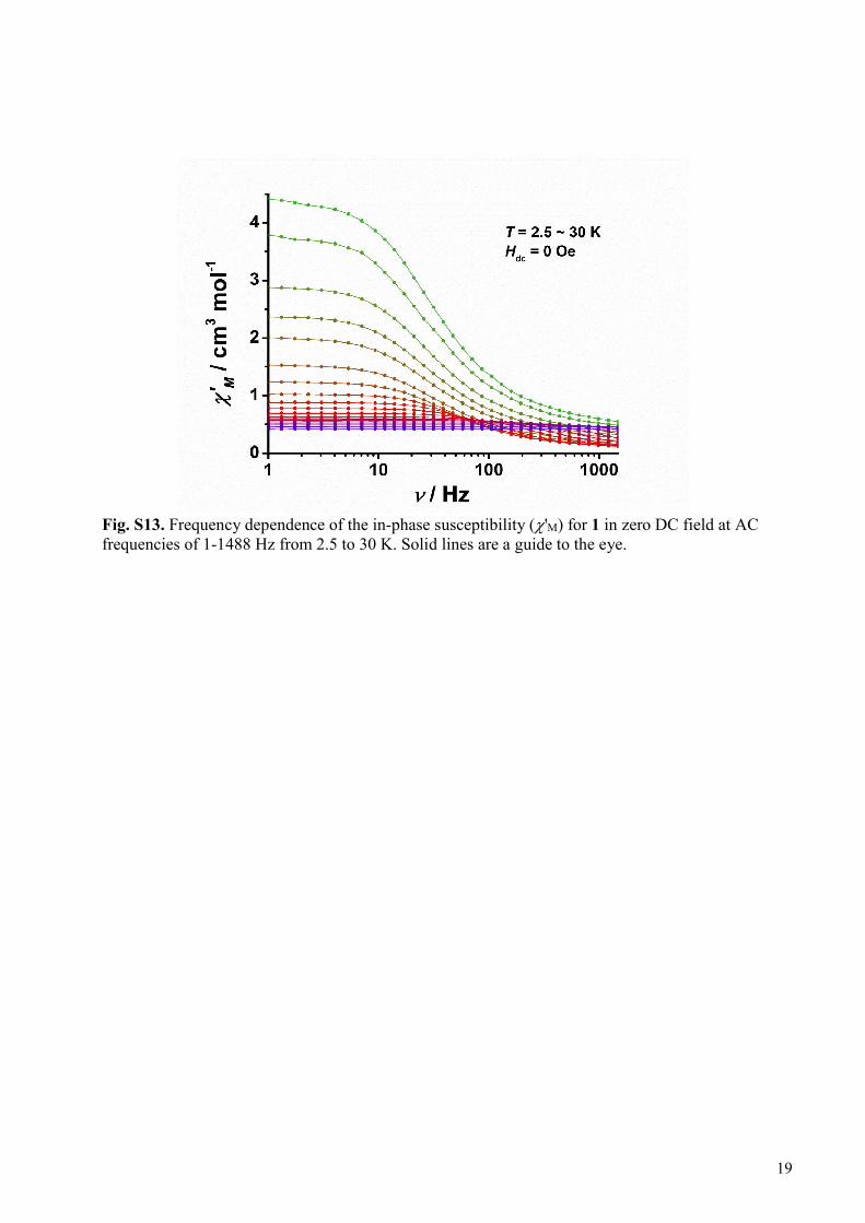
Fig. S13. Frequency dependence of the in-phase susceptibility ('M) for 1 in zero DC field at AC frequencies of 1-1488 Hz from 2.5 to 30 K. Solid lines are a guide to the eye.
19
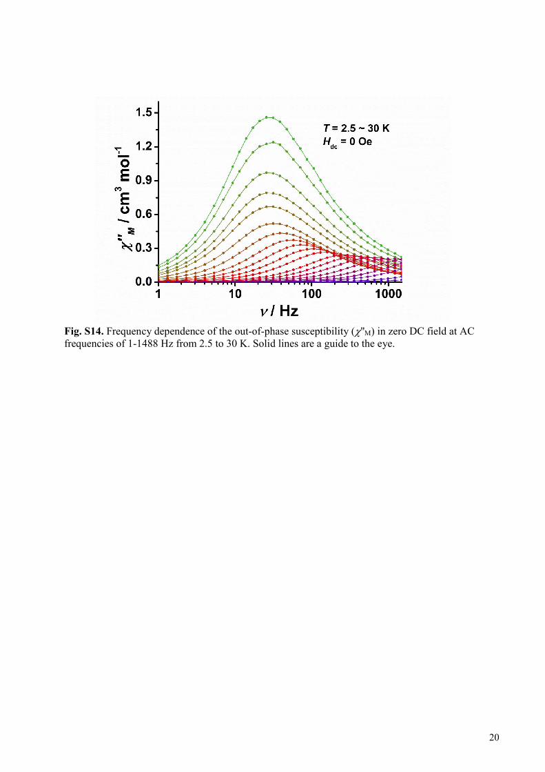
Fig. S14. Frequency dependence of the out-of-phase susceptibility (''M) in zero DC field at AC frequencies of 1-1488 Hz from 2.5 to 30 K. Solid lines are a guide to the eye.
20
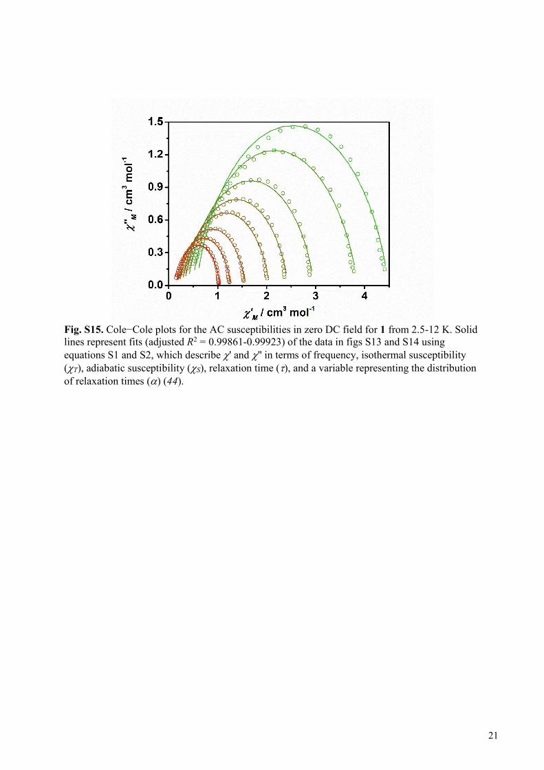
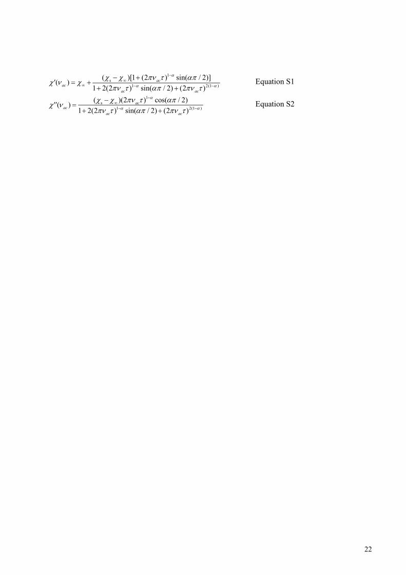
Fig. S15. Cole−Cole plots for the AC susceptibilities in zero DC field for 1 from 2.5-12 K. Solid lines represent fits (adjusted R2 = 0.99861-0.99923) of the data in figs S13 and S14 using equations S1 and S2, which describe ' and '' in terms of frequency, isothermal susceptibility (T), adiabatic susceptibility (S), relaxation time (), and a variable representing the distribution of relaxation times () (44).
21
1s
1 2(1 )
( )[1 (2 ) sin( / 2)]( )
1 2(2 ) sin( / 2) (2 )ac
ac
ac ac
'
Equation S1
1s
1 2(1 )
( )(2 ) cos( / 2)( )
1 2(2 ) sin( / 2) (2 )ac
ac
ac ac
''
Equation S2
22
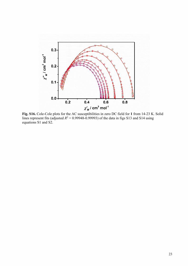
Fig. S16. Cole-Cole plots for the AC susceptibilities in zero DC field for 1 from 14-23 K. Solid lines represent fits (adjusted R2 = 0.99948-0.99993) of the data in figs S13 and S14 using equations S1 and S2.
23
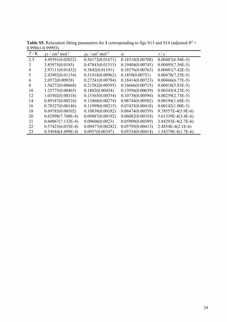
Table S5. Relaxation fitting parameters for 1 corresponding to figs S13 and S14 (adjusted R2 = 0.99861-0.99993).
T / K T / cm3 mol-1 S / cm3 mol-1 / s
2.5 4.49391(0.02022) 0.56172(0.01671) 0.18318(0.00708) 0.00487(6.94E-5) 3 3.85975(0.0185) 0.47843(0.01515) 0.19404(0.00745) 0.00495(7.56E-5) 4 2.97111(0.01432) 0.3842(0.01191) 0.18576(0.00763) 0.00481(7.42E-5) 5 2.43992(0.01154) 0.31918(0.00962) 0.1859(0.00751) 0.00478(7.25E-5) 6 2.0572(0.00928) 0.27241(0.00784) 0.18414(0.00723) 0.00466(6.77E-5) 8 1.56272(0.00668) 0.21582(0.00595) 0.16666(0.00715) 0.00418(5.83E-5) 10 1.25775(0.00465) 0.1802(0.00454) 0.13956(0.00659) 0.00345(4.23E-5) 12 1.03502(0.00318) 0.15365(0.00354) 0.10738(0.00594) 0.00259(2.73E-5) 14 0.89187(0.00216) 0.13468(0.00274) 0.08744(0.00502) 0.00194(1.68E-5) 16 0.78327(0.00146) 0.11999(0.00215) 0.07435(0.00418) 0.00142(1.00E-5) 18 0.69785(0.00102) 0.10838(0.00182) 0.06474(0.00359) 9.78557E-4(5.9E-6) 20 0.62998(7.760E-4) 0.09887(0.00192) 0.06082(0.00354) 5.61539E-4(3.4E-6) 21 0.60067(7.132E-4) 0.09606(0.0023) 0.05909(0.00389) 3.84293E-4(2.7E-6) 22 0.57423(6.035E-4) 0.09477(0.00282) 0.05795(0.00413) 2.4854E-4(2.1E-6) 23 0.54944(4.499E-4) 0.0957(0.00347) 0.05334(0.00414) 1.54379E-4(1.7E-6)
24
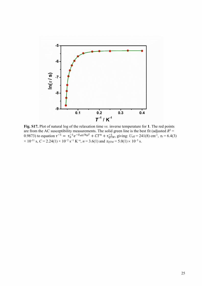
Fig. S17. Plot of natural log of the relaxation time vs. inverse temperature for 1. The red points are from the AC susceptibility measurements. The solid green line is the best fit (adjusted R2 = 0.9873) to equation ��� = ��
��������/��� + ��� + ������ , giving: Ueff = 241(8) cm-1, 0 = 6.4(3)
× 10-11 s, C = 2.24(1) × 10−2 s−1 K−n, n = 3.6(1) and QTM = 5.0(1) 10–3 s.
25
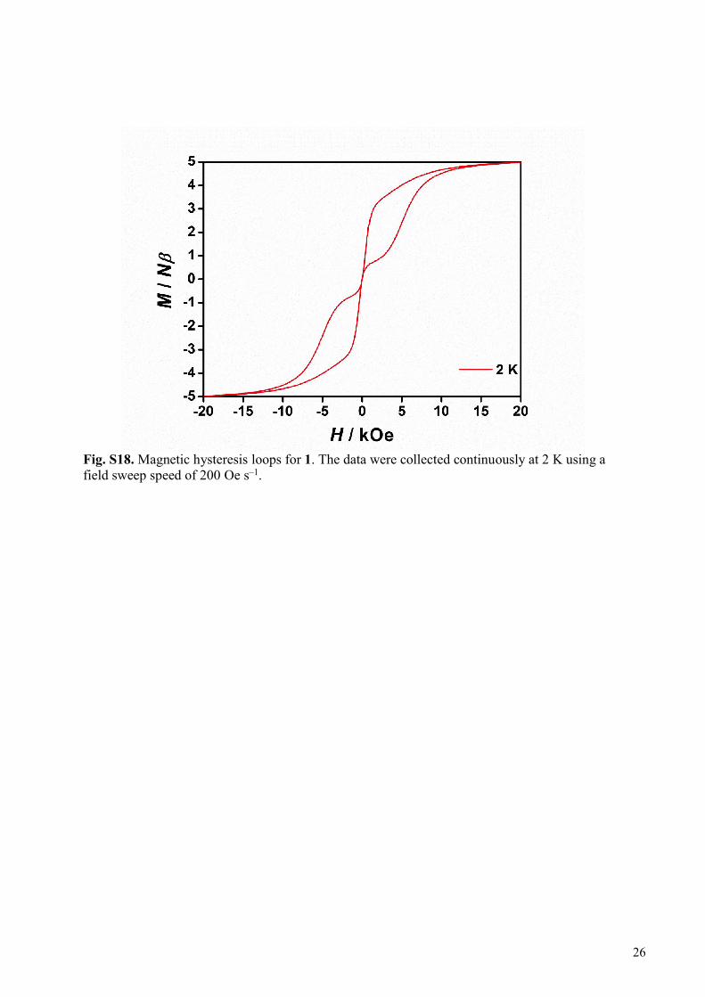
Fig. S18. Magnetic hysteresis loops for 1. The data were collected continuously at 2 K using a field sweep speed of 200 Oe s–1.
26
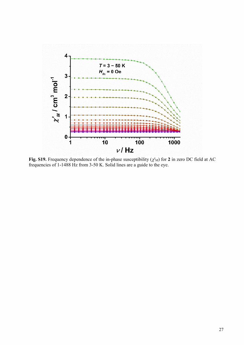
Fig. S19. Frequency dependence of the in-phase susceptibility ('M) for 2 in zero DC field at AC frequencies of 1-1488 Hz from 3-50 K. Solid lines are a guide to the eye.
27
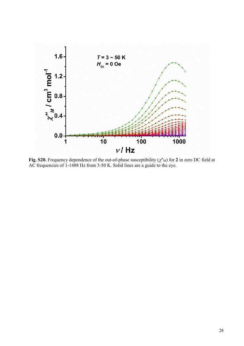
Fig. S20. Frequency dependence of the out-of-phase susceptibility (''M) for 2 in zero DC field at AC frequencies of 1-1488 Hz from 3-50 K. Solid lines are a guide to the eye.
28
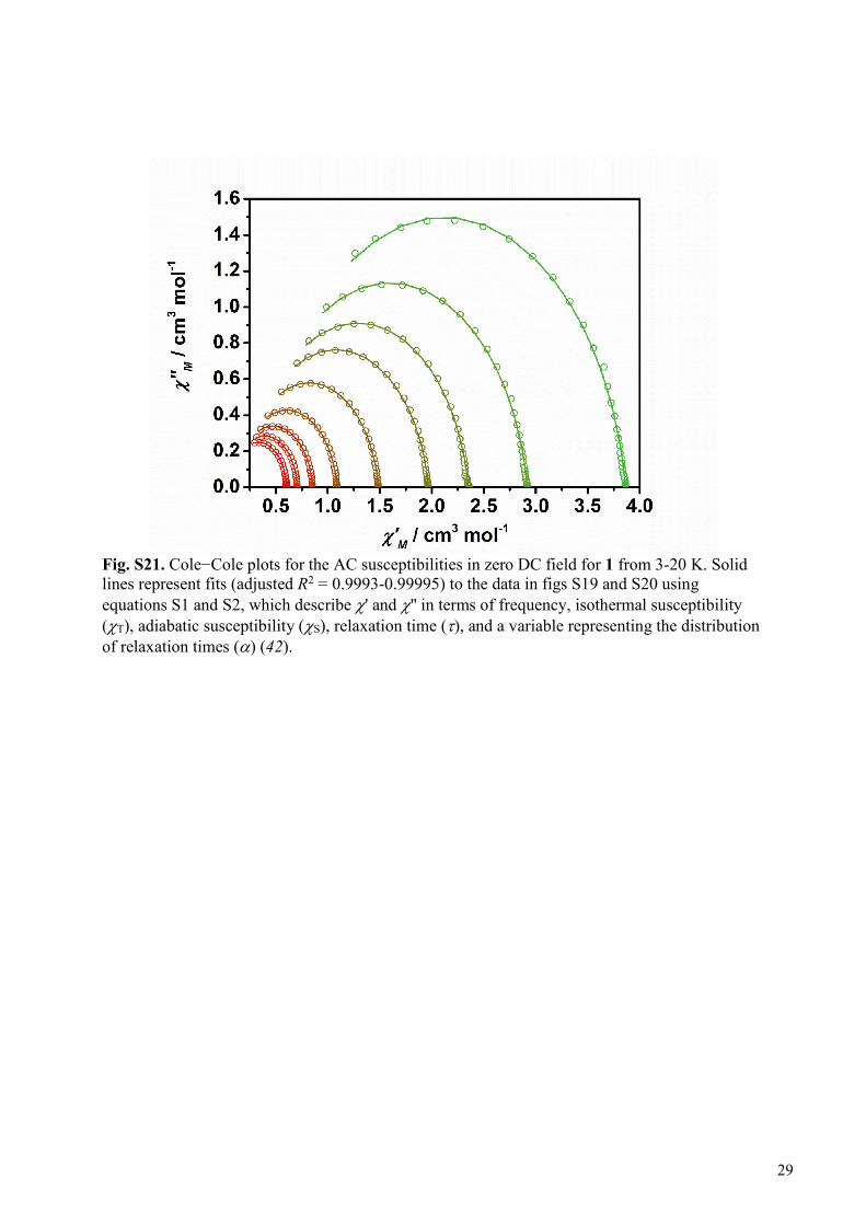
Fig. S21. Cole−Cole plots for the AC susceptibilities in zero DC field for 1 from 3-20 K. Solid lines represent fits (adjusted R2 = 0.9993-0.99995) to the data in figs S19 and S20 using equations S1 and S2, which describe ' and '' in terms of frequency, isothermal susceptibility (T), adiabatic susceptibility (S), relaxation time (), and a variable representing the distribution of relaxation times () (42).
29
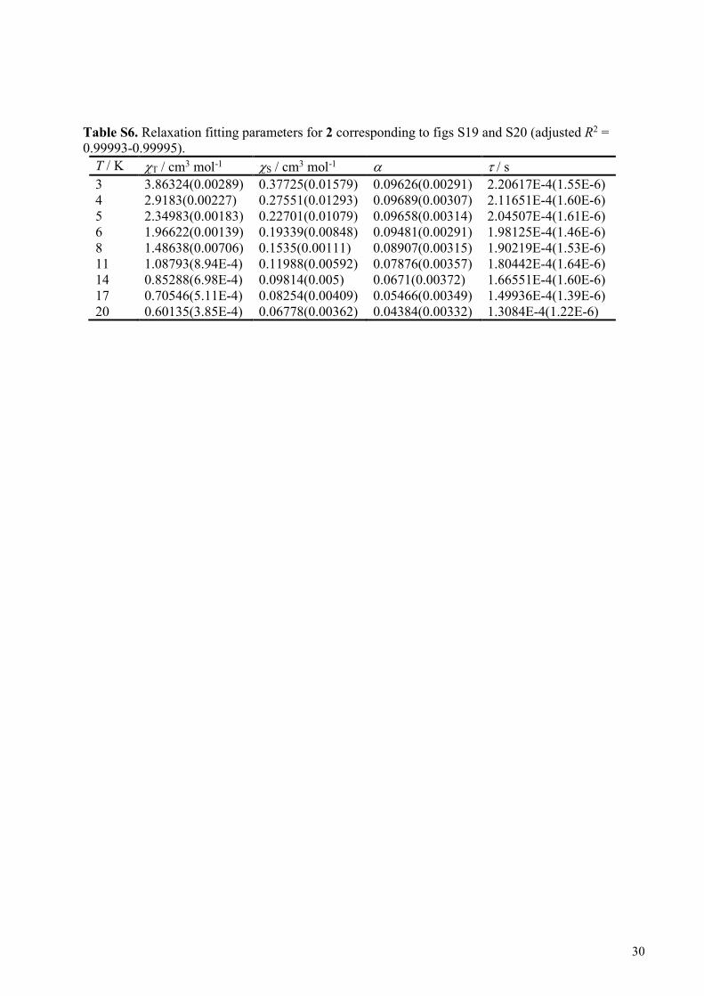
Table S6. Relaxation fitting parameters for 2 corresponding to figs S19 and S20 (adjusted R2 = 0.99993-0.99995).
T / K T / cm3 mol-1 S / cm3 mol-1 / s
3 3.86324(0.00289) 0.37725(0.01579) 0.09626(0.00291) 2.20617E-4(1.55E-6) 4 2.9183(0.00227) 0.27551(0.01293) 0.09689(0.00307) 2.11651E-4(1.60E-6) 5 2.34983(0.00183) 0.22701(0.01079) 0.09658(0.00314) 2.04507E-4(1.61E-6) 6 1.96622(0.00139) 0.19339(0.00848) 0.09481(0.00291) 1.98125E-4(1.46E-6) 8 1.48638(0.00706) 0.1535(0.00111) 0.08907(0.00315) 1.90219E-4(1.53E-6) 11 1.08793(8.94E-4) 0.11988(0.00592) 0.07876(0.00357) 1.80442E-4(1.64E-6) 14 0.85288(6.98E-4) 0.09814(0.005) 0.0671(0.00372) 1.66551E-4(1.60E-6) 17 0.70546(5.11E-4) 0.08254(0.00409) 0.05466(0.00349) 1.49936E-4(1.39E-6) 20 0.60135(3.85E-4) 0.06778(0.00362) 0.04384(0.00332) 1.3084E-4(1.22E-6)
30
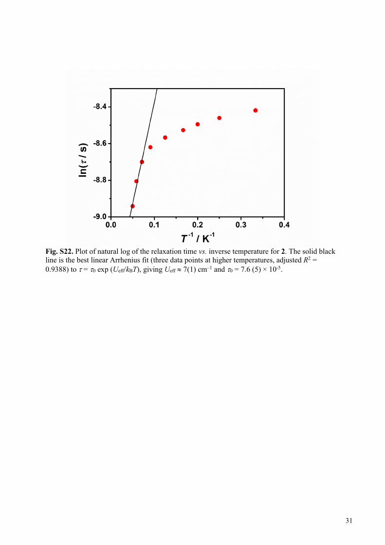
Fig. S22. Plot of natural log of the relaxation time vs. inverse temperature for 2. The solid black line is the best linear Arrhenius fit (three data points at higher temperatures, adjusted R2 = 0.9388) to = 0 exp (Ueff/kBT), giving Ueff 7(1) cm–1 and 0 = 7.6 (5) × 10-5.
31

Fig. S23. Magnetic hysteresis loops for 2. The data were continuously collected at 2 K under a field sweep speed of 200 Oe s–1.
32
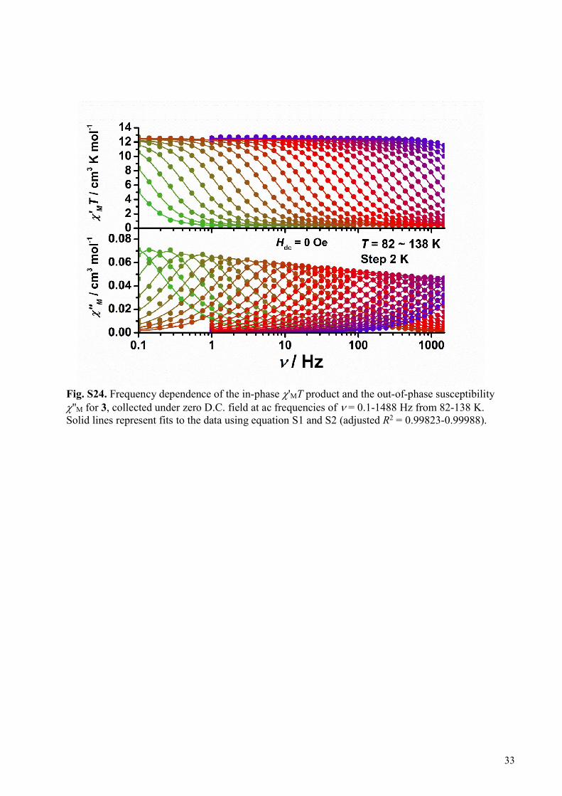
Fig. S24. Frequency dependence of the in-phase 'MT product and the out-of-phase susceptibility ''M for 3, collected under zero D.C. field at ac frequencies of = 0.1-1488 Hz from 82-138 K. Solid lines represent fits to the data using equation S1 and S2 (adjusted R2 = 0.99823-0.99988).
33
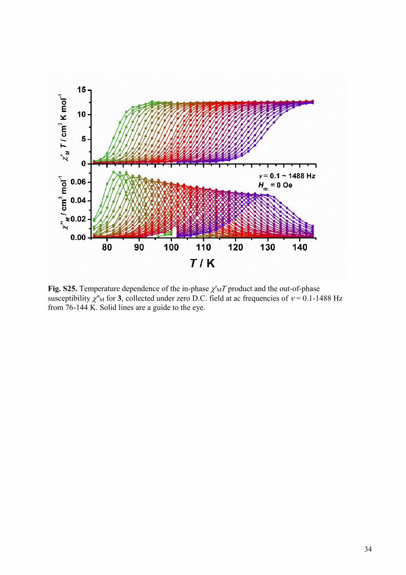
Fig. S25. Temperature dependence of the in-phase 'MT product and the out-of-phase susceptibility ''M for 3, collected under zero D.C. field at ac frequencies of = 0.1-1488 Hz from 76-144 K. Solid lines are a guide to the eye.
34
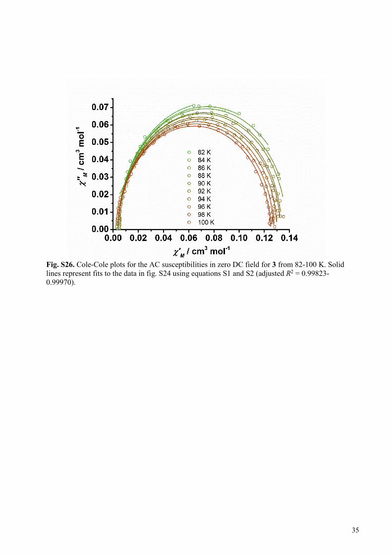
Fig. S26. Cole-Cole plots for the AC susceptibilities in zero DC field for 3 from 82-100 K. Solid lines represent fits to the data in fig. S24 using equations S1 and S2 (adjusted R2 = 0.99823-0.99970).
35
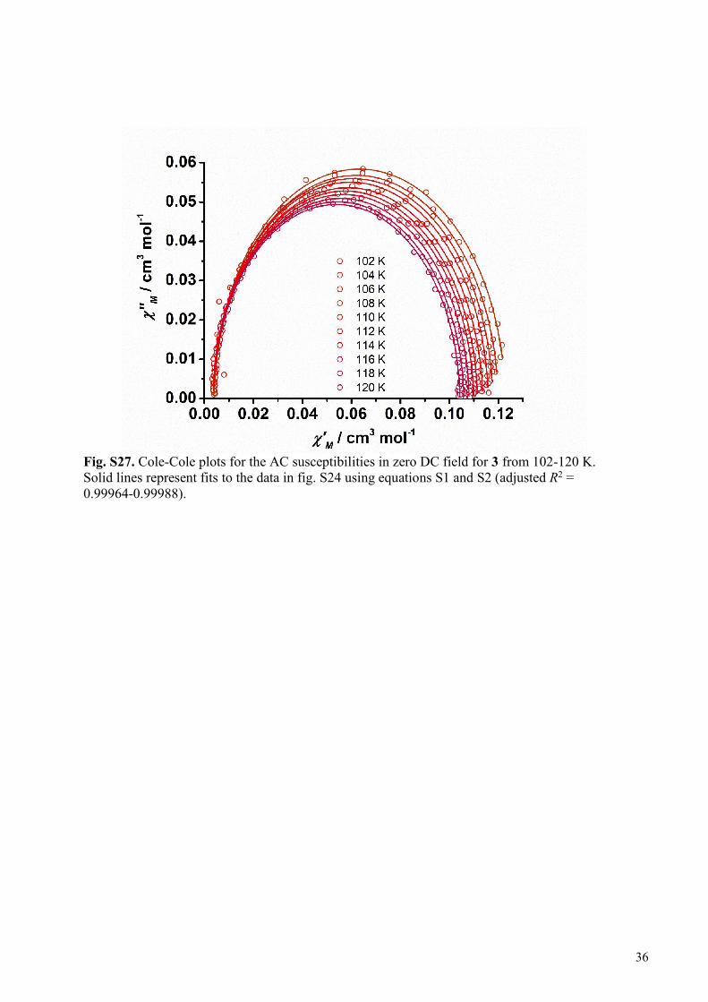
Fig. S27. Cole-Cole plots for the AC susceptibilities in zero DC field for 3 from 102-120 K. Solid lines represent fits to the data in fig. S24 using equations S1 and S2 (adjusted R2 = 0.99964-0.99988).
36
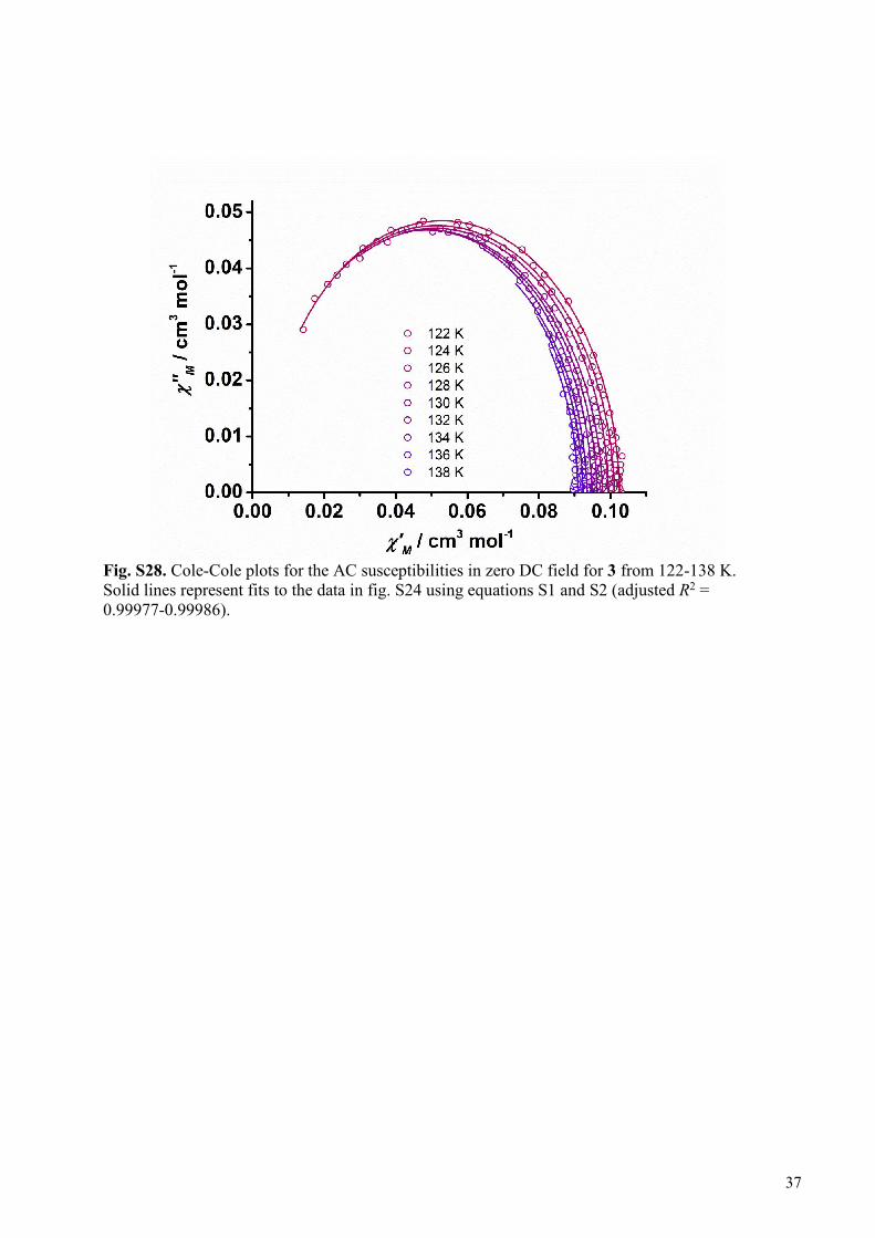
Fig. S28. Cole-Cole plots for the AC susceptibilities in zero DC field for 3 from 122-138 K. Solid lines represent fits to the data in fig. S24 using equations S1 and S2 (adjusted R2 = 0.99977-0.99986).
37
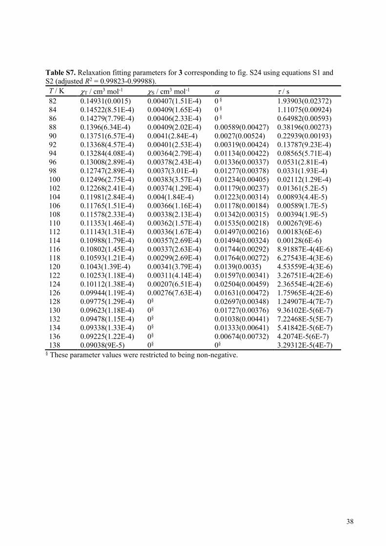
Table S7. Relaxation fitting parameters for 3 corresponding to fig. S24 using equations S1 and S2 (adjusted R2 = 0.99823-0.99988).
T / K T / cm3 mol-1 S / cm3 mol-1 / s
82 0.14931(0.0015) 0.00407(1.51E-4) 0 § 1.93903(0.02372) 84 0.14522(8.51E-4) 0.00409(1.65E-4) 0 § 1.11075(0.00924) 86 0.14279(7.79E-4) 0.00406(2.33E-4) 0 § 0.64982(0.00593) 88 0.1396(6.34E-4) 0.00409(2.02E-4) 0.00589(0.00427) 0.38196(0.00273) 90 0.13751(6.57E-4) 0.0041(2.84E-4) 0.0027(0.00524) 0.22939(0.00193) 92 0.13368(4.57E-4) 0.00401(2.53E-4) 0.00319(0.00424) 0.13787(9.23E-4) 94 0.13284(4.08E-4) 0.00364(2.79E-4) 0.01134(0.00422) 0.08565(5.71E-4) 96 0.13008(2.89E-4) 0.00378(2.43E-4) 0.01336(0.00337) 0.0531(2.81E-4) 98 0.12747(2.89E-4) 0.0037(3.01E-4) 0.01277(0.00378) 0.0331(1.93E-4) 100 0.12496(2.75E-4) 0.00383(3.57E-4) 0.01234(0.00405) 0.02112(1.29E-4) 102 0.12268(2.41E-4) 0.00374(1.29E-4) 0.01179(0.00237) 0.01361(5.2E-5) 104 0.11981(2.84E-4) 0.004(1.84E-4) 0.01223(0.00314) 0.00893(4.4E-5) 106 0.11765(1.51E-4) 0.00366(1.16E-4) 0.01178(0.00184) 0.00589(1.7E-5) 108 0.11578(2.33E-4) 0.00338(2.13E-4) 0.01342(0.00315) 0.00394(1.9E-5) 110 0.11353(1.46E-4) 0.00362(1.57E-4) 0.01535(0.00218) 0.00267(9E-6) 112 0.11143(1.31E-4) 0.00336(1.67E-4) 0.01497(0.00216) 0.00183(6E-6) 114 0.10988(1.79E-4) 0.00357(2.69E-4) 0.01494(0.00324) 0.00128(6E-6) 116 0.10802(1.45E-4) 0.00337(2.63E-4) 0.01744(0.00292) 8.91887E-4(4E-6) 118 0.10593(1.21E-4) 0.00299(2.69E-4) 0.01764(0.00272) 6.27543E-4(3E-6) 120 0.1043(1.39E-4) 0.00341(3.79E-4) 0.0139(0.0035) 4.53559E-4(3E-6) 122 0.10253(1.18E-4) 0.00311(4.14E-4) 0.01597(0.00341) 3.26751E-4(2E-6) 124 0.10112(1.38E-4) 0.00207(6.51E-4) 0.02504(0.00459) 2.36554E-4(2E-6) 126 0.09944(1.19E-4) 0.00276(7.63E-4) 0.01631(0.00472) 1.75965E-4(2E-6) 128 0.09775(1.29E-4) 0§ 0.02697(0.00348) 1.24907E-4(7E-7) 130 0.09623(1.18E-4) 0§ 0.01727(0.00376) 9.36102E-5(6E-7) 132 0.09478(1.15E-4) 0§ 0.01038(0.00441) 7.22468E-5(5E-7) 134 0.09338(1.33E-4) 0§ 0.01333(0.00641) 5.41842E-5(6E-7) 136 0.09225(1.22E-4) 0§ 0.00674(0.00732) 4.2074E-5(6E-7) 138 0.09038(9E-5) 0§ 0§ 3.29312E-5(4E-7)
§ These parameter values were restricted to being non-negative.
38
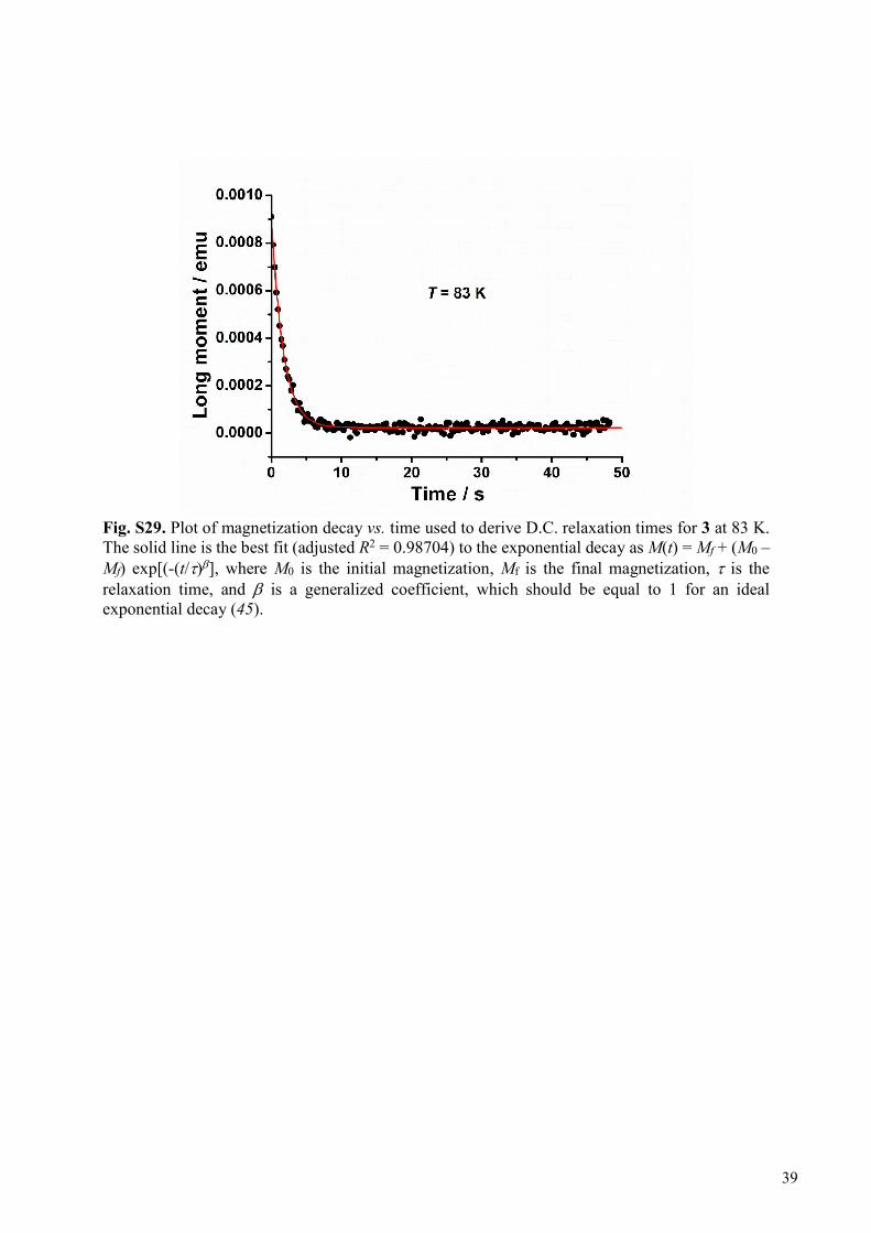
Fig. S29. Plot of magnetization decay vs. time used to derive D.C. relaxation times for 3 at 83 K. The solid line is the best fit (adjusted R2 = 0.98704) to the exponential decay as M(t) = Mf + (M0 – Mf) exp[(-(t/)], where M0 is the initial magnetization, Mf is the final magnetization, is the relaxation time, and is a generalized coefficient, which should be equal to 1 for an ideal exponential decay (45).
39
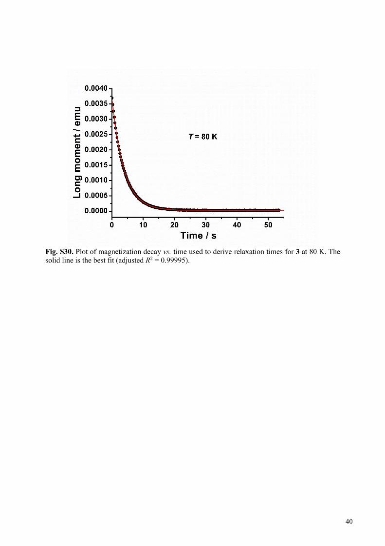
Fig. S30. Plot of magnetization decay vs. time used to derive relaxation times for 3 at 80 K. The solid line is the best fit (adjusted R2 = 0.99995).
40
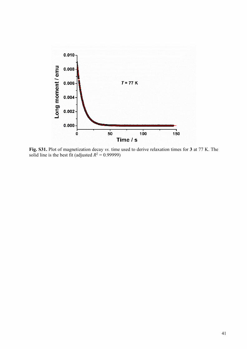
Fig. S31. Plot of magnetization decay vs. time used to derive relaxation times for 3 at 77 K. The solid line is the best fit (adjusted R2 = 0.99999)
41
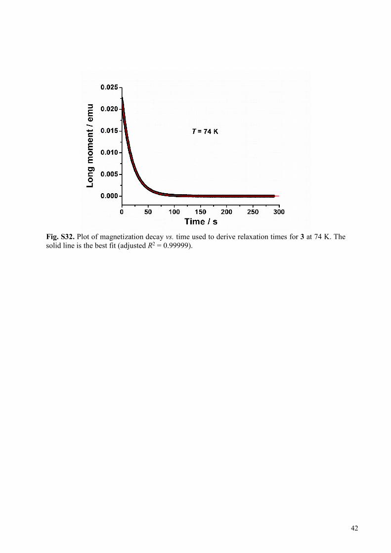
Fig. S32. Plot of magnetization decay vs. time used to derive relaxation times for 3 at 74 K. The solid line is the best fit (adjusted R2 = 0.99999).
42

Fig. S33. Plot of magnetization decay vs. time used to derive relaxation times for 3 at 70 K. The solid line is the best fit (adjusted R2 = 0.99999).
43
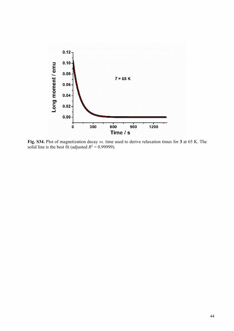
Fig. S34. Plot of magnetization decay vs. time used to derive relaxation times for 3 at 65 K. The solid line is the best fit (adjusted R2 = 0.99999).
44

Fig. S35. Plot of magnetization decay vs. time used to derive relaxation times for 3 at 60 K. The solid line is the best fit (adjusted R2 = 0.99999).
45

Fig. S36. Plot of magnetization decay vs. time used to derive relaxation times for 3 at 55 K. The solid line is the best fit (adjusted R2 = 0.99999).
46
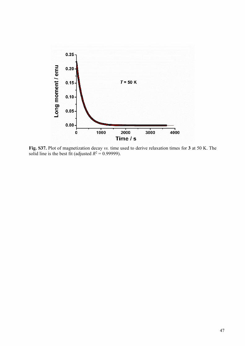
Fig. S37. Plot of magnetization decay vs. time used to derive relaxation times for 3 at 50 K. The solid line is the best fit (adjusted R2 = 0.99999).
47
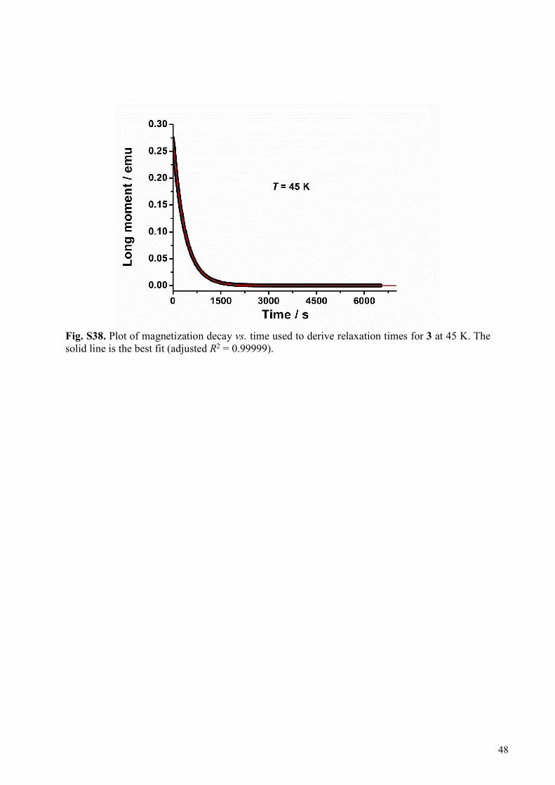
Fig. S38. Plot of magnetization decay vs. time used to derive relaxation times for 3 at 45 K. The solid line is the best fit (adjusted R2 = 0.99999).
48

Fig. S39. Plot of magnetization decay vs. time used to derive relaxation times for 3 at 40 K. The solid line is the best fit (adjusted R2 = 0.99999).
49
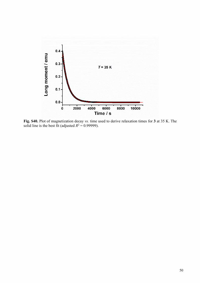
Fig. S40. Plot of magnetization decay vs. time used to derive relaxation times for 3 at 35 K. The solid line is the best fit (adjusted R2 = 0.99999).
50
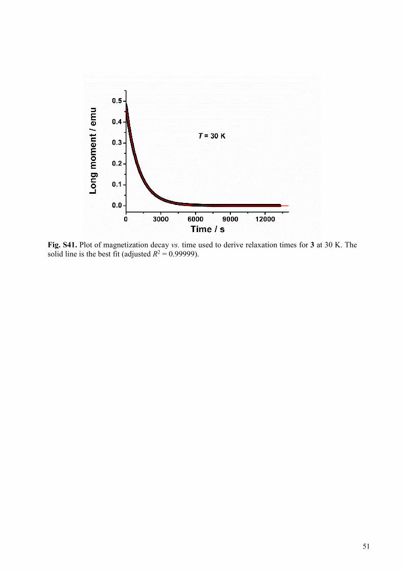
Fig. S41. Plot of magnetization decay vs. time used to derive relaxation times for 3 at 30 K. The solid line is the best fit (adjusted R2 = 0.99999).
51
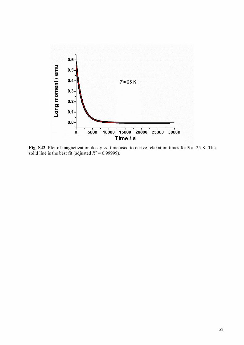
Fig. S42. Plot of magnetization decay vs. time used to derive relaxation times for 3 at 25 K. The solid line is the best fit (adjusted R2 = 0.99999).
52
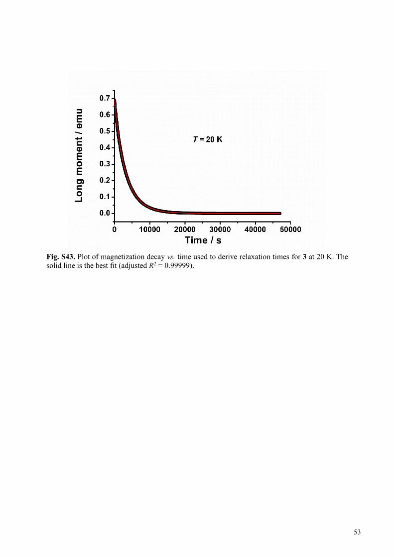
Fig. S43. Plot of magnetization decay vs. time used to derive relaxation times for 3 at 20 K. The solid line is the best fit (adjusted R2 = 0.99999).
53

Fig. S44. Plot of magnetization decay vs. time used to derive relaxation times for 3 at 15 K. The solid line is the best fit (adjusted R2 = 0.99999).
54
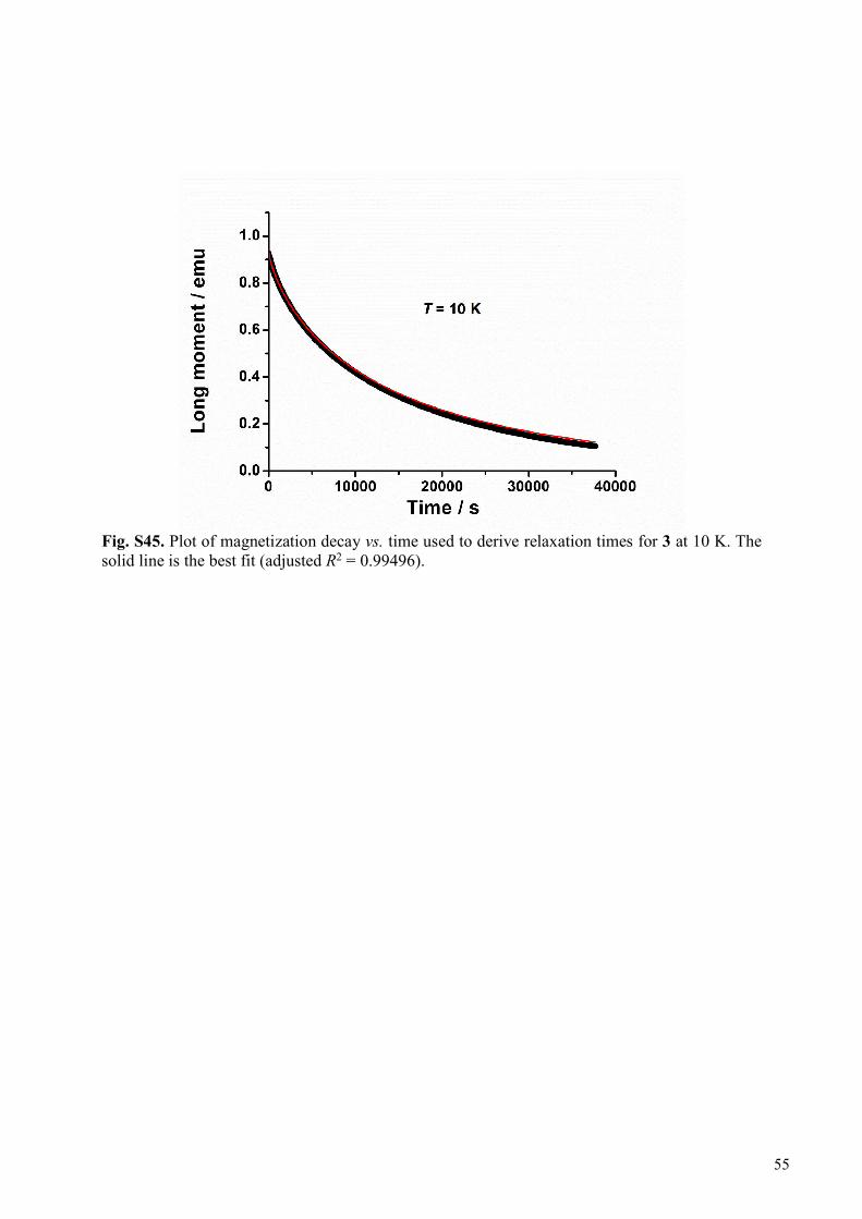
Fig. S45. Plot of magnetization decay vs. time used to derive relaxation times for 3 at 10 K. The solid line is the best fit (adjusted R2 = 0.99496).
55
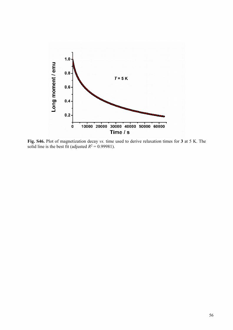
Fig. S46. Plot of magnetization decay vs. time used to derive relaxation times for 3 at 5 K. The solid line is the best fit (adjusted R2 = 0.99981).
56

Fig. S47. Plot of magnetization decay vs. time used to derive relaxation times for 3 at 3 K. The solid line is the best fit (adjusted R2 = 0.99988).
57
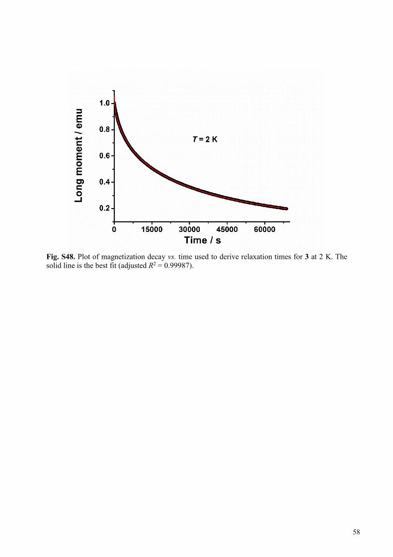
Fig. S48. Plot of magnetization decay vs. time used to derive relaxation times for 3 at 2 K. The solid line is the best fit (adjusted R2 = 0.99987).
58
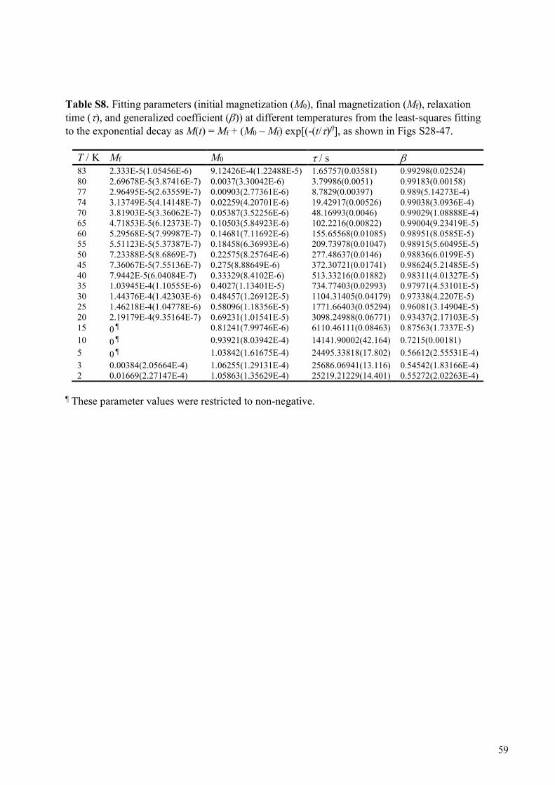
Table S8. Fitting parameters (initial magnetization (M0), final magnetization (Mf), relaxation time (), and generalized coefficient ()) at different temperatures from the least-squares fitting to the exponential decay as M(t) = Mf + (M0 – Mf) exp[(-(t/)], as shown in Figs S28-47.
T / K Mf M0 / s 83 2.333E-5(1.05456E-6) 9.12426E-4(1.22488E-5) 1.65757(0.03581) 0.99298(0.02524) 80 2.69678E-5(3.87416E-7) 0.0037(3.30042E-6) 3.79986(0.0051) 0.99183(0.00158) 77 2.96495E-5(2.63559E-7) 0.00903(2.77361E-6) 8.7829(0.00397) 0.989(5.14273E-4) 74 3.13749E-5(4.14148E-7) 0.02259(4.20701E-6) 19.42917(0.00526) 0.99038(3.0936E-4) 70 3.81903E-5(3.36062E-7) 0.05387(3.52256E-6) 48.16993(0.0046) 0.99029(1.08888E-4) 65 4.71853E-5(6.12373E-7) 0.10503(5.84923E-6) 102.2216(0.00822) 0.99004(9.23419E-5) 60 5.29568E-5(7.99987E-7) 0.14681(7.11692E-6) 155.65568(0.01085) 0.98951(8.0585E-5) 55 5.51123E-5(5.37387E-7) 0.18458(6.36993E-6) 209.73978(0.01047) 0.98915(5.60495E-5) 50 7.23388E-5(8.6869E-7) 0.22575(8.25764E-6) 277.48637(0.0146) 0.98836(6.0199E-5) 45 7.36067E-5(7.55136E-7) 0.275(8.88649E-6) 372.30721(0.01741) 0.98624(5.21485E-5) 40 7.9442E-5(6.04084E-7) 0.33329(8.4102E-6) 513.33216(0.01882) 0.98311(4.01327E-5) 35 1.03945E-4(1.10555E-6) 0.4027(1.13401E-5) 734.77403(0.02993) 0.97971(4.53101E-5) 30 1.44376E-4(1.42303E-6) 0.48457(1.26912E-5) 1104.31405(0.04179) 0.97338(4.2207E-5) 25 1.46218E-4(1.04778E-6) 0.58096(1.18356E-5) 1771.66403(0.05294) 0.96081(3.14904E-5) 20 2.19179E-4(9.35164E-7) 0.69231(1.01541E-5) 3098.24988(0.06771) 0.93437(2.17103E-5) 15 0 ¶ 0.81241(7.99746E-6) 6110.46111(0.08463) 0.87563(1.7337E-5)
10 0 ¶ 0.93921(8.03942E-4) 14141.90002(42.164) 0.7215(0.00181)
5 0 ¶ 1.03842(1.61675E-4) 24495.33818(17.802) 0.56612(2.55531E-4)
3 0.00384(2.05664E-4) 1.06255(1.29131E-4) 25686.06941(13.116) 0.54542(1.83166E-4) 2 0.01669(2.27147E-4) 1.05863(1.35629E-4) 25219.21229(14.401) 0.55272(2.02263E-4)
¶ These parameter values were restricted to non-negative.
59
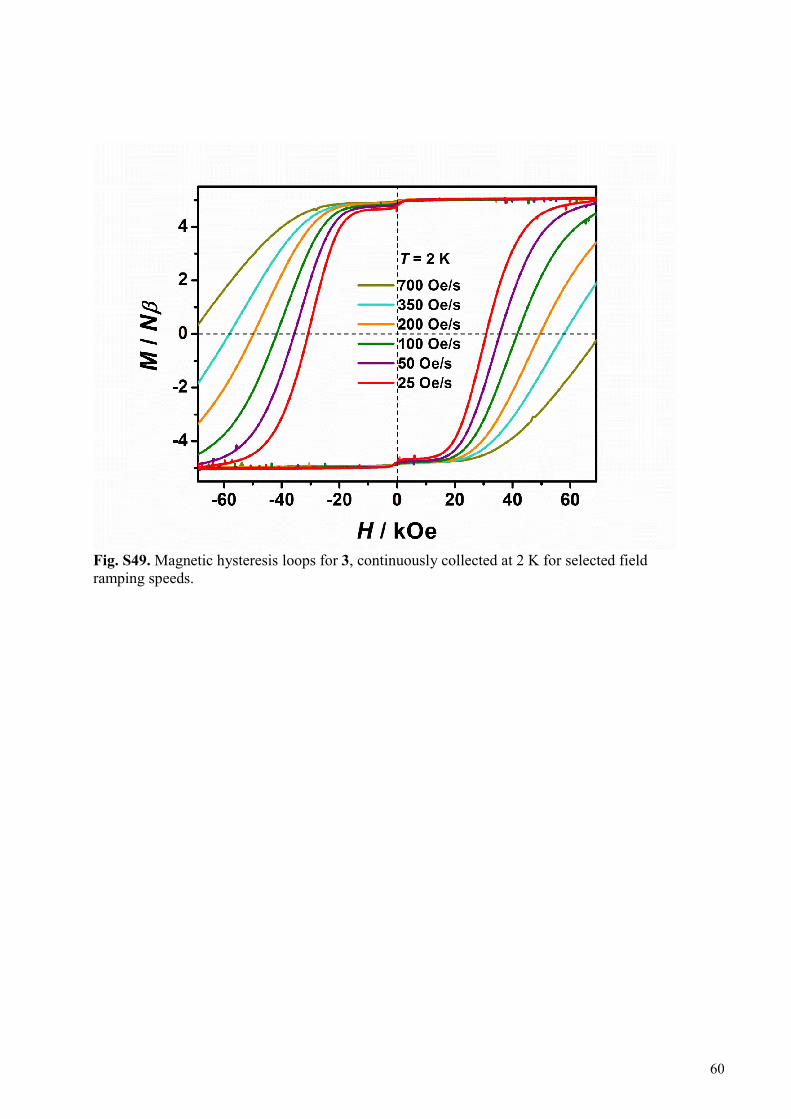
Fig. S49. Magnetic hysteresis loops for 3, continuously collected at 2 K for selected field ramping speeds.
60
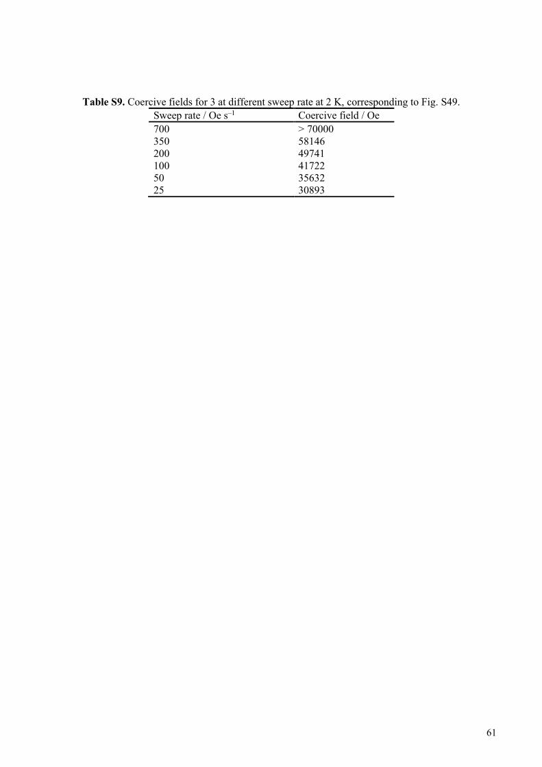
Table S9. Coercive fields for 3 at different sweep rate at 2 K, corresponding to Fig. S49.
Sweep rate / Oe s–1 Coercive field / Oe
700 > 70000 350 58146 200 49741 100 41722 50 35632 25 30893
61
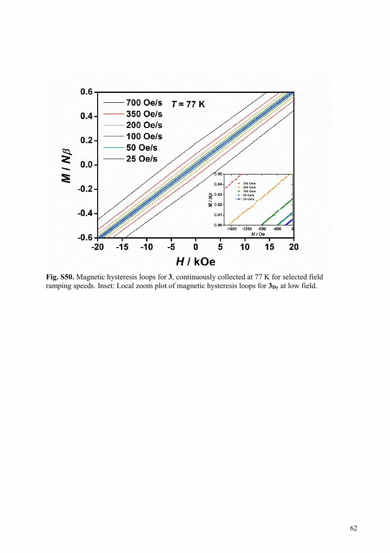
Fig. S50. Magnetic hysteresis loops for 3, continuously collected at 77 K for selected field ramping speeds. Inset: Local zoom plot of magnetic hysteresis loops for 3Dy at low field.
62
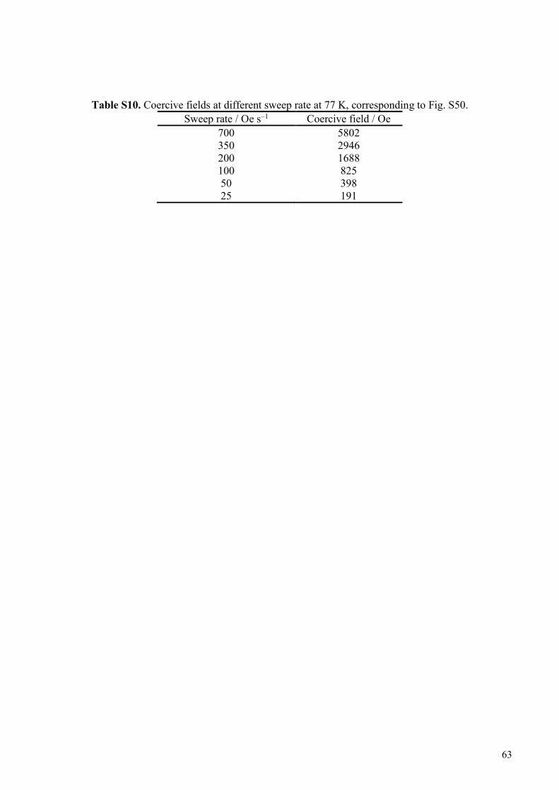
Table S10. Coercive fields at different sweep rate at 77 K, corresponding to Fig. S50.
Sweep rate / Oe s–1 Coercive field / Oe
700 5802 350 2946 200 1688 100 825 50 398 25 191
63
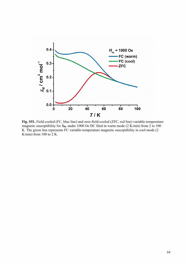
Fig. S51. Field-cooled (FC, blue line) and zero-field-cooled (ZFC, red line) variable-temperature magnetic susceptibility for 3Dy under 1000 Oe DC filed in warm mode (2 K/min) from 2 to 100 K. The green line represents FC variable-temperature magnetic susceptibility in cool mode (2 K/min) from 100 to 2 K.
64
Supplementary text: Computational details: The static electronic structure was calculated using the multireference XMS-CASPT2//SA-CASSCF/RASSI approach (33, 34) and the Molcas quantum chemistry code version 8.2 (46). The geometry was extracted from the crystal-structure and the positions of the hydrogen atoms were optimized at density function theory (DFT) level using the same level of theory as in the frequency calculations (vide infra) while the coordinates of the heavier atoms were fixed to their XRD-determined positions. The nine 4f electrons and the seven 4f orbitals of the Dy(III) ion were used as the active space. Relativistically contracted atomic natural orbital (ANO-RCC) basis sets were used throughout (47, 48). A polarized valence quadruple-ζ quality (ANO-RCC-QZVP, [9s8p6d4f3g2h] contraction) basis set was used for the Dy(III) ion, polarized valence triple-ζ quality (ANO-RCC-VTZP, [4s3p2d1f] contraction) basis set was used for the carbon atoms in the Cp rings, and polarized valence double-ζ quality (ANO-RCC-VDZP, [3s2p1d] and [2s1p] contractions) basis sets were used for the other C and H atoms. Scalar relativistic effects were treated using the exact two-component (X2C) transformation (49-51) as implemented in Molcas. Cholesky decomposition using a threshold of 10-8 was used to reduce the storage size of the two-electron integrals. Three separate state-averaged (SA) complete active space self-consistent field (CASSCF) calculations (52-55) were carried out to solve the 21 sextet, 228 quartet, and 490 doublet roots. Then, a series of extended multistate (XMS) complete active space perturbation theory at second order (CASPT2) calculations were conducted on the lowest 21 sextet, 128 quartet, and 130 doublet states corresponding to an energy cut-off of 50,000 cm–1 at CASSCF level. The XMS version (30) of the well-known CASPT2 approach (56-59) was chosen to avoid artificial splitting of spatially degenerate or near-degenerate states observed in the conventional multistate CASPT2 approach (59). The XMS-CASPT2 corrections were only calculated to the eigenvalues and no mixing of the CASSCF eigenstates under dynamic electron correlation was taken into account (the “NOMULT” keyword in Molcas). The states chosen into each XMS group correspond to some term or closely spaced group of terms of the free Dy(III) ion. A total of three groups containing 11, 7, and 3 CASSCF states were used for the sextets, twelve groups were containing 13, 7, 19, 9, 15, 17, 5, 11, 3, 9, 7, and 13 CASSCF states were used for the quartet CASSCF states, and ten groups containing 17, 15, 3, 21, 7, 19, 11, 5, 9, and 23 states were used for the doublets. Finally, all states used in the XMS-CASPT2 calculations were mixed by spin-orbit coupling (SOC) using the well-established restricted active space state interaction (RASSI) approach (60). The static magnetic properties (g-tensors, magnetic susceptibility, and magnetization) were calculated using the SINGLE_ANISO routine (31, 60, 61) The CF parameters were calculated using the ab-initio crystal-field approach (33, 34) as implemented in SINGLE_ANISO. The vibrational modes were calculated at DFT level using the Gaussian 09 code revision D.01 (62). The PBE0 hybrid exchange-correlation functional (63-66) was used along with Ahlrichs’ TZVP basis sets (67). A 4f-in-core effective core potential (ECP), which treated the inner 55 electrons as an effective potential, along with a core-polarized valence triple-ζ quality basis was used for the Dy(III) ion (68-71). The geometry was fully optimized without any constraints. Dispersion effects were introduced using the empirical DFT-D3 dispersion correction (72) with
65
the Becke-Johnson damping function (73) The “UltraFine” integration grid (99 radial points and 590 angular points per atom) and “tight” convergence criteria (thresholds 1.5 · 10–5, 1.0 · 10–5, 6.0 · 10–5, and 4.0 · 10–5 for maximum force, RMS, force, maximum displacement, and RMS displacement, respectively) were used in Gaussian. All normal modes correspond to bound vibrations. The differentials of the CF parameters were calculated using single point-calculations at XMS-CASPT2//CASSCF/RASSI level on geometries generated by displacing the equilibrium structure along the normal modes. The total displacement (i.e. the sum of all displaced distances) was normalized to 2.0 Å. Several different values of this number were tried in preliminary calculations to minimize the numerical error and to maximize the stability of the numerical derivatives with respect to small variations of the normalized distance. Two displacements (positive and negative) were used for each normal mode, and the first derivatives of the CF parameters were evaluated using a finite difference method (symmetric derivative). The level of theory in the single point ab initio calculations was lowered somewhat to reduce the overall computational costs. The basis set was reduced so that the Dy(III) ion wast treated with a polarized valence triple-ζ quality (ANO-RCC-VTZP) basis set, the carbon atoms in the cyclopentadienyl rings were treated with a polarized valence double-ζ quality (ANO-RCC-VTZP, [8s7p5d3f2g1h] contraction) basis set, and the other atoms were treated with double-ζ (ANO-RCC-VDZ, [3s2p] and [2s] contractions for C and H, respectively) basis sets. In the CASSCF calculations and the subsequent XMS-CASPT2 and RASSI calculations, only the 21 sextet states were considered. This approximation does introduce some error but should still yield results very close to those obtained at a considerably higher cost by calculating also the quartet and doublet states. With the exception of the simplifications listed above, the single-point calculations were carried out at the same level as the calculations on the static electronic structure. The generation of the displaced geometries and the subsequent calculations of the derivatives was carried out using a custom code. The ab initio CF parameters were calculated for the Dy-5* cation following previously established methodology (32, 33). The CF parameters that normally correspond to Stevens’ original definition of operator equivalents (written as ����
� (��)) were converted to the newer Iwahara-Chibotaru
definition (written as ����(��)) of the CF Hamiltonian (74, 75):
,���� = ∑ �������(��)�� = ∑ ���������
� (��)
���� (�)
(1)
where Bkq are the CF parameters and ���� (�) is obtained from ����
� ���� by the replacement ��� → �.
The ranks, k, are even numbers and run up to 2J. The components q run from –k to k for each rank k. The newer definition of the operator equivalents has several advantages over the conventional definition; namely, the matrix elements of the operators are always of order unity and the magnitudes of the parameters are therefore easy to compare between different operator ranks. Furthermore, a simple general expression is available for the matrix elements, and the magnitudes of the CF parameters are symmetric in q: |Bkq| = |Bk–q|. The main disadvantage of the definition is that the off-diagonal CF parameters are complex. We are, however, mostly interested in the magnitudes of the parameters as these enter the expressions for the transition probabilities (vide infra).
66
The first- and second-order contributions of optical phonons to the electronic part of the spin-phonon coupling Hamiltonian can be estimated as (75, 76):
����(�)
= ∑ �� ∑ �����
����
��������(��)��� (2)
,����(�)
= ∑ ���� ∑ ������
�������
��,��������(��)���� (3)
where Qn is displacement along the nth normal mode, Bkq are CF parameters in the Iwahara–Chibotaru definition, and ����(��) are operator equivalents in the Iwahara–Chibotaru definition. The
transition probabilities between CF states |�⟩ and |��⟩ following the direct, first-order Raman, and second-order Raman mechanisms, in that order, are given by (43, 75, 77):
�(� ← ��) =��
ħ���������
(�)�����
�
�(�), (4)
�(� ← ��) =��
ħ� ��������(�)
������
�(�), and (5)
�(� ← ��) =��
ħ��
�������(�)
���′���′′�����(�)
����
��
�
�(�), (6)
where ħ is the reduced Planck constant, �(�) is a factor depending on the vibrational modes and the energy difference between the states |�⟩ and |��⟩, |��′⟩ is an intermediate state in the first-order Raman process, and Δ is the energy of the intermediate state relative to the initial state. Thus, in each case the spin-phonon transition probability is proportional to the matrix elements of the first- or second-order spin-phonon coupling Hamiltonian. The actual Orbach process consists of several consecutive direct transitions. The normal modes of Dy-5* were calculated at density functional theory (DFT) level and the respective frequencies are listed in Table S15. This introduces some approximation as the geometry must be optimized and a gas-phase optimization necessarily excludes crystal-packing effects. Furthermore, the effect of 4f configuration and 4f–ligand covalency were neglected in the calculations as these are difficult to treat at DFT-level. The optimized bond distances between the Dy ion and the centroids of the Cp* and CpiPr5 rings are 2.322 Å and 2.304 Å, respectively, and the Cp*–Dy–CpiPr5 angle is 158.42°. The respective experimentally determined parameters are 2.296(1) Å, 2.284(1) Å, and 162.507(1) Å. Although, the geometric parameters are qualitatively similar, the calculated bond-lengths are overestimated roughly by 0.02 Å most likely due to the fact that the 4f–ligand covalency is neglected. The calculated bend angle is also slightly more acute. Although the errors in the bond lengths are less than a percent and the error in the bend angle is less than three percent, these deviations are large enough to cause quantitative errors in the calculated CF parameters. To analyze the extent to which different approximation in the calculations affect the results, the CF splitting of the ground 6H15/2 multiplet was calculated on the optimized geometry using the same level of theory used in the evaluation of the spin-phonon couplings (see section
67
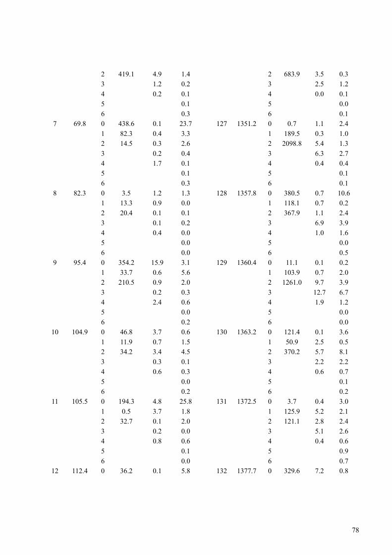
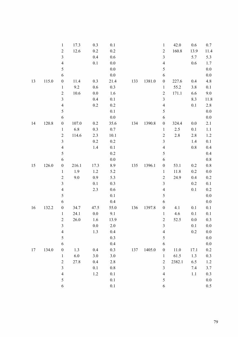
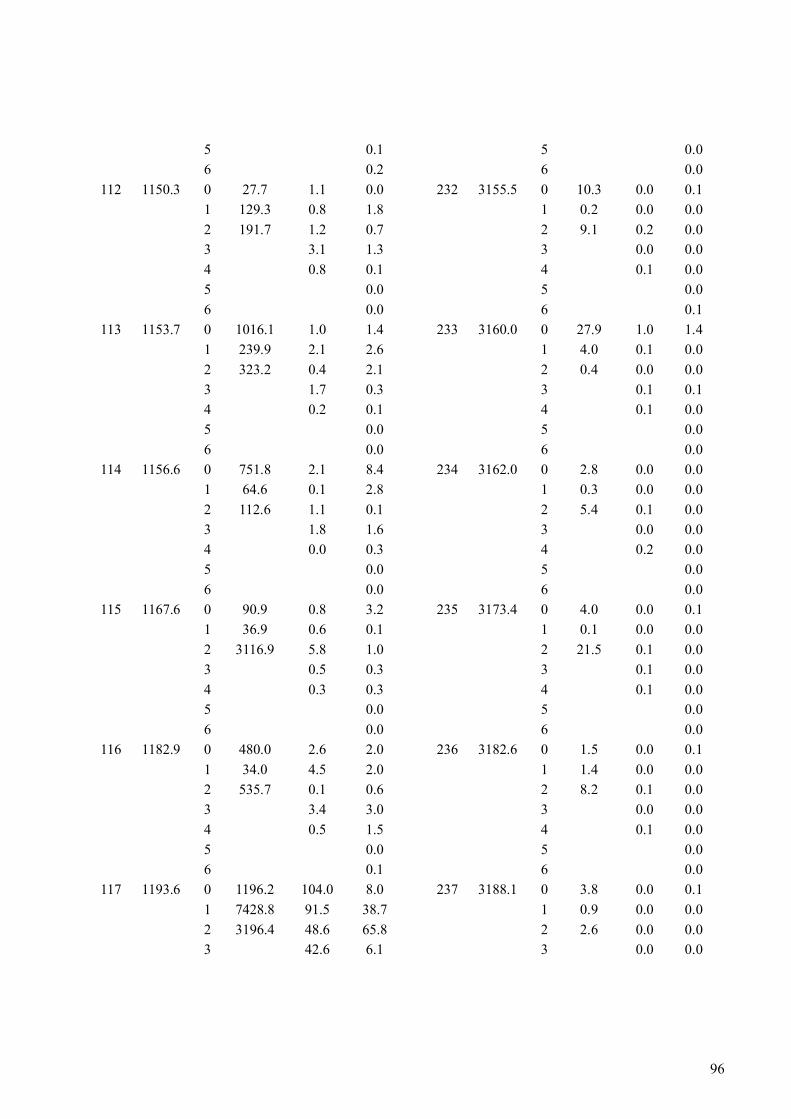
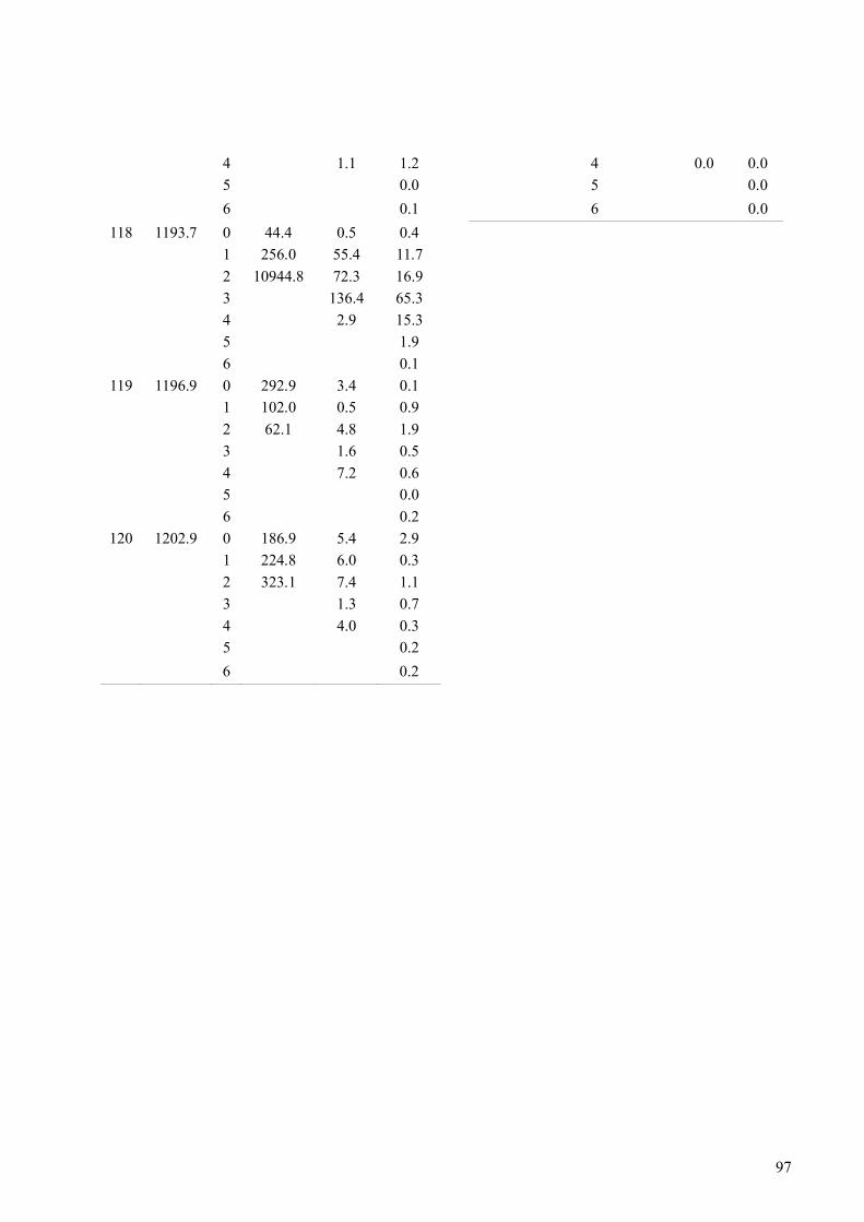
Computational details for further details). The results are listed in Table S16. The CF splitting calculated on the DFT-optimized geometry is roughly 75% of that calculated on the crystal structure geometry. This is consistent with the overestimated Dy–ligand distances. Despite these errors, the splitting is still qualitatively correct, and since the evaluation of derivatives concerns energy differences of slightly distorted structures, most of the error present in the absolute values of the splittings should cancel, and the evaluated energy differences should be much more accurate than the absolute splittings. Thus, the 25% error in the splittings defines the maximum error in the derivatives and the actual errors should be much smaller. It is therefore reasonable to assume that the errors originating from the DFT optimization are not much larger than the errors originating from assuming that the molecular vibrations are an approximation of the optical phonons. The first derivatives of the CF parameters with respect to each of the 237 normal modes of Dy-5* were numerically evaluated by single point calculations at XMS-CASPT2//SA-CASSCF/SO-RASSI level on geometries displaced in positive and negative directions along the normal modes. Evaluation of the second derivatives, although in principle possible, is unfeasible in terms of computational time required. Thus, the vibrational contributions to first-order Raman relaxation were not evaluated. Only operator equivalents up to rank k = 6 were considered. In principle, operators up to rank k = 14 can make contributions and the derivatives were calculated, but the small values of the respective CF parameters and resulting derivatives makes it impossible to reliably distinguish the values from numerical noise. Since only the magnitudes of the derivatives enter the final relaxation rate expressions, only these are considered, and since |Bkq| = |Bk–q|, only positives values of q are listed. The squared magnitudes of the first derivatives are listed in Table S17. It is clear that the largest derivatives are those of the 2nd rank parameters and, thus, these terms in the operator lead to the largest matrix elements and the first-order (non-Raman) relaxation can be qualitatively understood by considering the 2nd rank terms only. The states in the lowest six doublets have very large projections on some |��⟩ state, and can be, to a first approximation, considered as pure |��⟩ states: |�⟩ ∼ |��⟩ and |�′⟩ ∼ |��′⟩. Then, the ���±�(��) operators induce
direct transitions between two |��⟩ states differing by Δ� = � − �� = ±2, the ���±�(��) operators
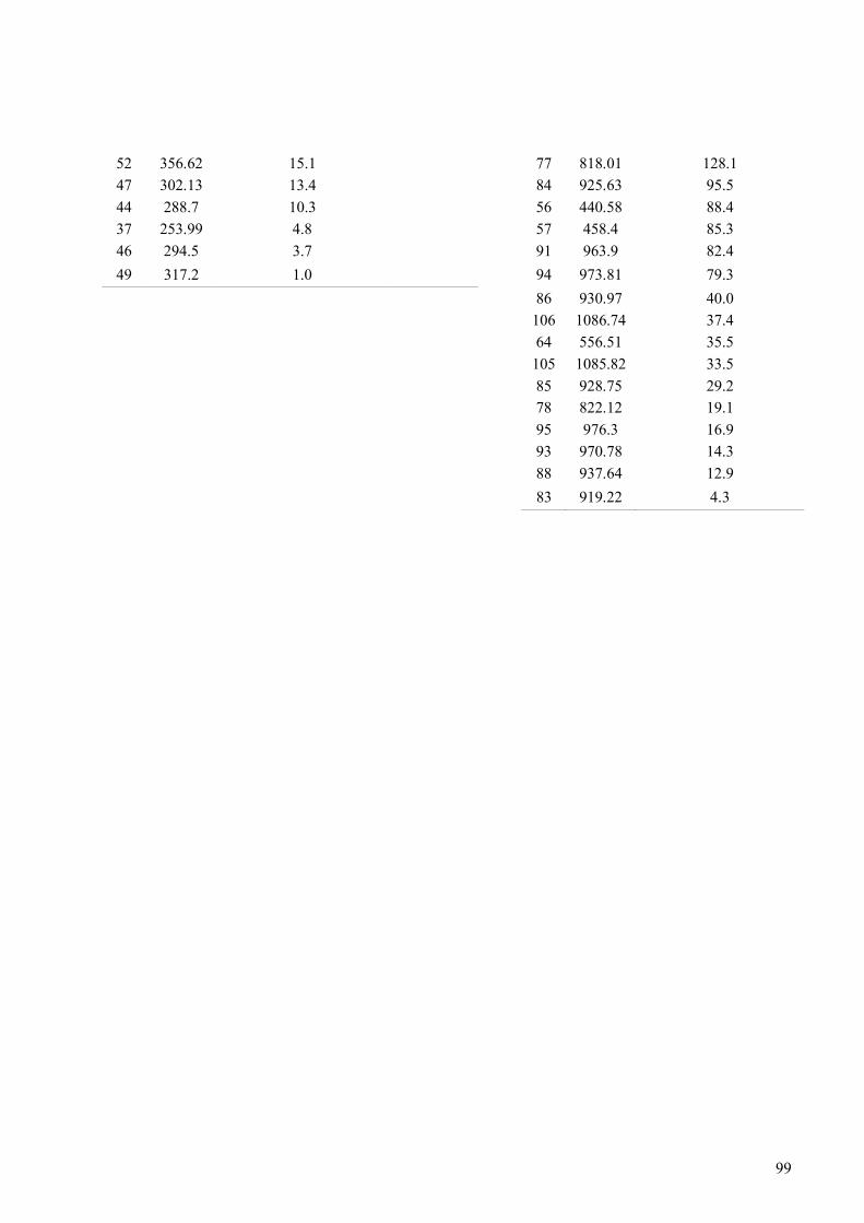
induce transitions between neighboring states differing by Δ� = ±1, and the ����(��) operator does not induce any transitions. If one confines themselves to the lowest six doublets (the seventh and eighth doublets do not take part in the Orbach process based on the experimental effective barrier height and on the extent of QTM due to the transverse components of the g-tensors), the energy range of the Δ� = ±1 transitions (the energy difference between the relevant doublets) ranges from 432 cm–1 to 1061 cm–1 and the energy range of the Δ� = ±2 transitions from 212 cm–1 to 672 cm–1. The normal modes within these energy scales causing the largest spin-phonon couplings
����±�/���� and ����±�/���
� are listed in Table S18.
Examining the values in Table S18, the respective vibrational modes, and confining the analysis
to vibrational modes that cause spin-phonon couplings larger than ����±�/����
= 1000 and
����±�/����
= 1000, all relevant spin-phonon couplings are associated to vibrational modes of
the Cp cores of the CpiPr5 and Cp* ligands. Only the modes 75 and 98 are mostly confined to the iPr5 and CH3 groups, respectively, with minor coupling to the Cp ring vibrations. The largest
����±�/���� couplings are caused by rocking vibrations where the Cp core rocks relative to the
68
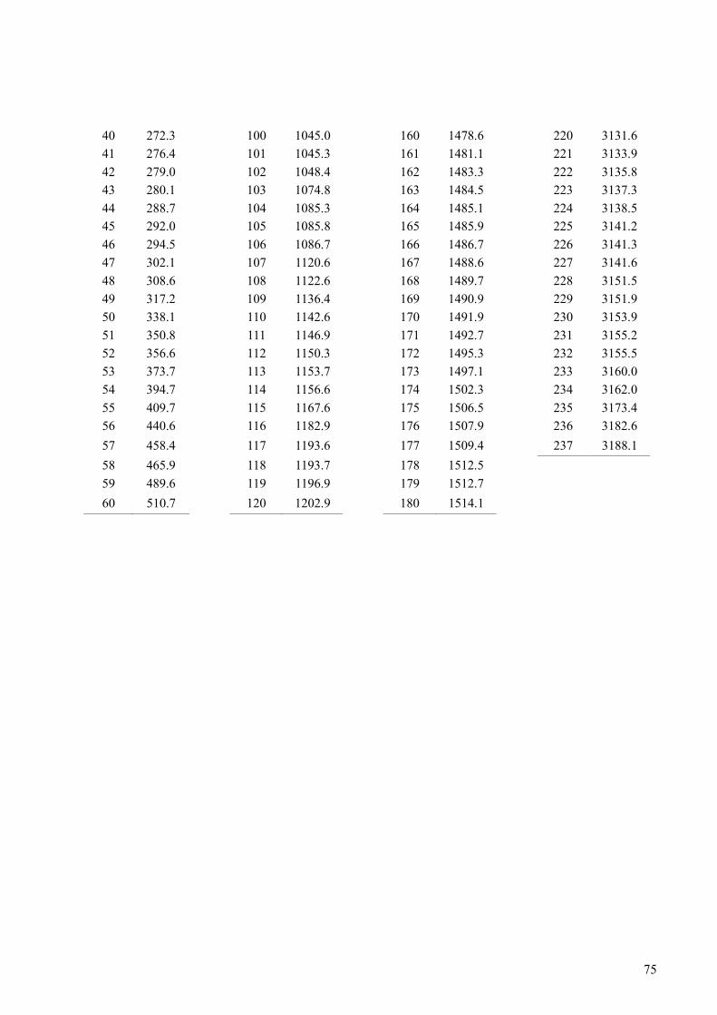
rest of the molecular structure. The modes 54 and 55, which cause the most significant spin-phonon couplings, are associated to rocking of the Cp core of the Cp* ligand and the modes 67 and 68 are associated to the rocking of the Cp core of the CpiPr5 ligand. The modes 70 and 71 are out-of-plane vibrations of the Cp* ligand with significant coupling with CH3 vibrations and mode 66
corresponds to a symmetric in-plane stretching vibration of the CpiPr5 ligand. The ����±�/����
couplings are caused by a variety of modes including in-plane asymmetric vibrations of the CpiPr5 ligand (modes 73, 97, and 100) and the Cp* ligand (mode 62); out-of-plane vibrations of the CpiPr5 ligand (modes 70, 74, and 75) and the Cp* ligand (modes 71); in-plane symmetric vibrations of the CpiPr5 ligand (modes 79) and the Cp* ligand (modes 63, 90, 92); and rocking of the CpiPr5 ligand (modes 67 and 68) and the Cp* ligand (modes 54 and 55).
69
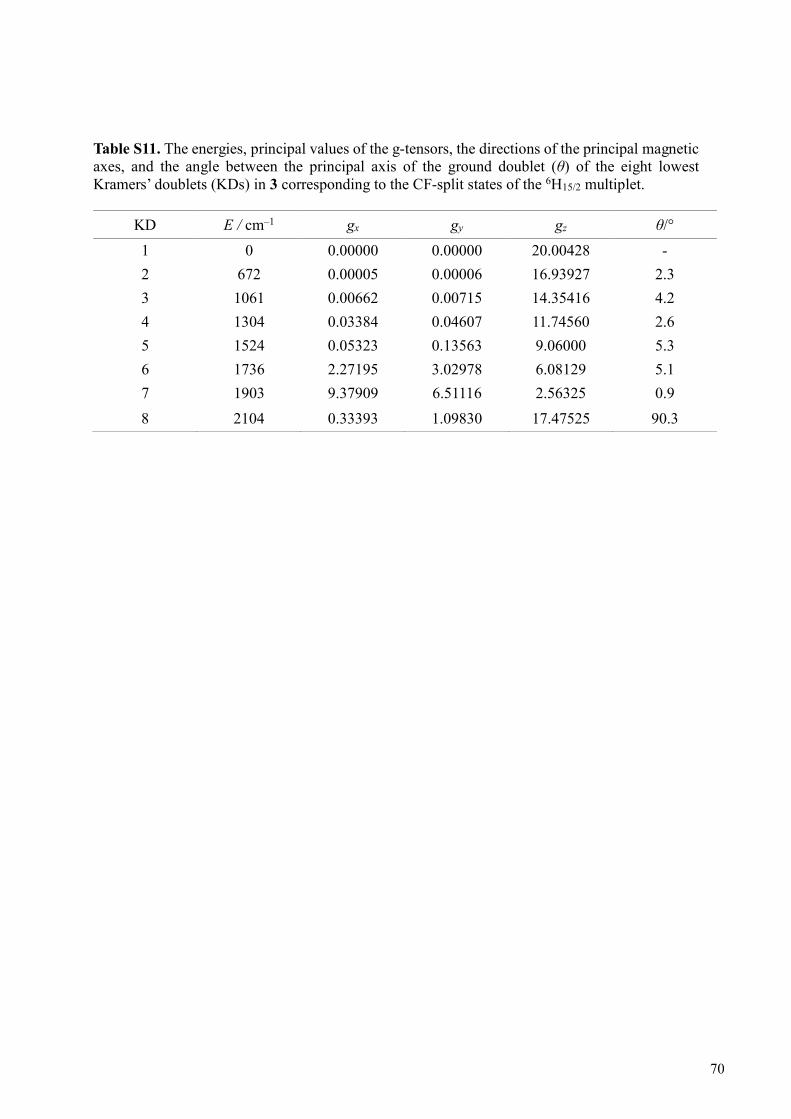
Table S11. The energies, principal values of the g-tensors, the directions of the principal magnetic axes, and the angle between the principal axis of the ground doublet (θ) of the eight lowest Kramers’ doublets (KDs) in 3 corresponding to the CF-split states of the 6H15/2 multiplet.
KD E / cm–1 gx gy gz θ/°
1 0 0.00000 0.00000 20.00428 -
2 672 0.00005 0.00006 16.93927 2.3
3 1061 0.00662 0.00715 14.35416 4.2
4 1304 0.03384 0.04607 11.74560 2.6
5 1524 0.05323 0.13563 9.06000 5.3
6 1736 2.27195 3.02978 6.08129 5.1
7 1903 9.37909 6.51116 2.56325 0.9
8 2104 0.33393 1.09830 17.47525 90.3
70
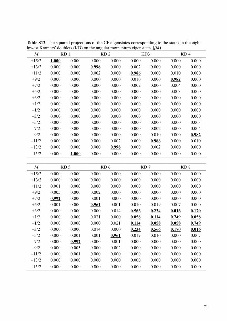
Table S12. The squared projections of the CF eigenstates corresponding to the states in the eight lowest Kramers’ doublets (KD) on the angular momentum eigenstates |��⟩.
M KD 1 KD 2 KD3 KD 4
+15/2 1.000 0.000 0.000 0.000 0.000 0.000 0.000 0.000
+13/2 0.000 0.000 0.998 0.000 0.002 0.000 0.000 0.000
+11/2 0.000 0.000 0.002 0.000 0.986 0.000 0.010 0.000
+9/2 0.000 0.000 0.000 0.000 0.010 0.000 0.982 0.000
+7/2 0.000 0.000 0.000 0.000 0.002 0.000 0.004 0.000
+5/2 0.000 0.000 0.000 0.000 0.000 0.000 0.003 0.000
+3/2 0.000 0.000 0.000 0.000 0.000 0.000 0.000 0.000
+1/2 0.000 0.000 0.000 0.000 0.000 0.000 0.000 0.000
–1/2 0.000 0.000 0.000 0.000 0.000 0.000 0.000 0.000
–3/2 0.000 0.000 0.000 0.000 0.000 0.000 0.000 0.000
–5/2 0.000 0.000 0.000 0.000 0.000 0.000 0.000 0.003
–7/2 0.000 0.000 0.000 0.000 0.000 0.002 0.000 0.004
–9/2 0.000 0.000 0.000 0.000 0.000 0.010 0.000 0.982
–11/2 0.000 0.000 0.000 0.002 0.000 0.986 0.000 0.010
–13/2 0.000 0.000 0.000 0.998 0.000 0.002 0.000 0.000
–15/2 0.000 1.000 0.000 0.000 0.000 0.000 0.000 0.000
M KD 5 KD 6 KD 7 KD 8
+15/2 0.000 0.000 0.000 0.000 0.000 0.000 0.000 0.000
+13/2 0.000 0.000 0.000 0.000 0.000 0.000 0.000 0.000
+11/2 0.001 0.000 0.000 0.000 0.000 0.000 0.000 0.000
+9/2 0.005 0.000 0.002 0.000 0.000 0.000 0.000 0.000
+7/2 0.992 0.000 0.001 0.000 0.000 0.000 0.000 0.000
+5/2 0.001 0.000 0.961 0.001 0.010 0.019 0.007 0.000
+3/2 0.000 0.000 0.000 0.014 0.566 0.234 0.016 0.170
+1/2 0.000 0.000 0.021 0.000 0.058 0.114 0.749 0.058
–1/2 0.000 0.000 0.000 0.021 0.114 0.058 0.058 0.749
–3/2 0.000 0.000 0.014 0.000 0.234 0.566 0.170 0.016
–5/2 0.000 0.001 0.001 0.961 0.019 0.010 0.000 0.007
–7/2 0.000 0.992 0.000 0.001 0.000 0.000 0.000 0.000
–9/2 0.000 0.005 0.000 0.002 0.000 0.000 0.000 0.000
–11/2 0.000 0.001 0.000 0.000 0.000 0.000 0.000 0.000
–13/2 0.000 0.000 0.000 0.000 0.000 0.000 0.000 0.000
–15/2 0.000 0.000 0.000 0.000 0.000 0.000 0.000 0.000
71
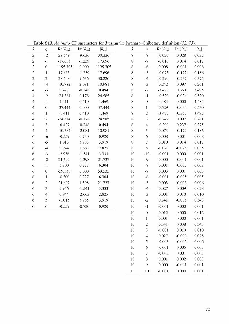
Table S13. Ab initio CF parameters for 3 using the Iwahara–Chibotaru definition (72, 73):
k q Re(Bkq) Im(Bkq) |Bkq| k q Re(Bkq) Im(Bkq) |Bkq|
2 -2 28.649 -9.636 30.226 8 -8 -0.020 0.028 0.035
2 -1 -17.653 -1.239 17.696 8 -7 -0.010 0.014 0.017
2 0 -1195.305 0.000 1195.305 8 -6 0.008 -0.001 0.008
2 1 17.653 -1.239 17.696 8 -5 -0.073 -0.172 0.186
2 2 28.649 9.636 30.226 8 -4 -0.290 -0.237 0.375
4 -4 -10.782 2.081 10.981 8 -3 0.242 0.097 0.261
4 -3 0.427 -0.248 0.494 8 -2 -3.477 0.360 3.495
4 -2 -24.584 0.178 24.585 8 -1 -0.529 -0.034 0.530
4 -1 1.411 0.410 1.469 8 0 4.484 0.000 4.484
4 0 -37.444 0.000 37.444 8 1 0.529 -0.034 0.530
4 1 -1.411 0.410 1.469 8 2 -3.477 -0.360 3.495
4 2 -24.584 -0.178 24.585 8 3 -0.242 0.097 0.261
4 3 -0.427 -0.248 0.494 8 4 -0.290 0.237 0.375
4 4 -10.782 -2.081 10.981 8 5 0.073 -0.172 0.186
6 -6 -0.559 0.730 0.920 8 6 0.008 0.001 0.008
6 -5 1.015 3.785 3.919 8 7 0.010 0.014 0.017
6 -4 0.944 2.663 2.825 8 8 -0.020 -0.028 0.035
6 -3 -2.956 -1.541 3.333 10 -10 -0.001 0.000 0.001
6 -2 21.692 -1.398 21.737 10 -9 0.000 -0.001 0.001
6 -1 6.300 0.227 6.304 10 -8 0.001 -0.002 0.003
6 0 -59.535 0.000 59.535 10 -7 0.003 0.001 0.003
6 1 -6.300 0.227 6.304 10 -6 -0.001 -0.005 0.005
6 2 21.692 1.398 21.737 10 -5 0.003 -0.005 0.006
6 3 2.956 -1.541 3.333 10 -4 0.027 0.009 0.028
6 4 0.944 -2.663 2.825 10 -3 0.001 0.010 0.010
6 5 -1.015 3.785 3.919 10 -2 0.341 -0.038 0.343
6 6 -0.559 -0.730 0.920 10 -1 -0.001 0.000 0.001
10 0 0.012 0.000 0.012
10 1 0.001 0.000 0.001
10 2 0.341 0.038 0.343
10 3 -0.001 0.010 0.010
10 4 0.027 -0.009 0.028
10 5 -0.003 -0.005 0.006
10 6 -0.001 0.005 0.005
10 7 -0.003 0.001 0.003
10 8 0.001 0.002 0.003
10 9 0.000 -0.001 0.001
10 10 -0.001 0.000 0.001
72
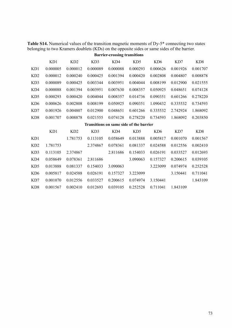
Table S14. Numerical values of the transition magnetic moments of Dy-5* connecting two states belonging to two Kramers doublets (KDs) on the opposite sides or same sides of the barrier.
Barrier-crossing transitions
KD1 KD2 KD3 KD4 KD5 KD6 KD7 KD8
KD1 0.000005 0.000012 0.000089 0.000088 0.000293 0.000626 0.001926 0.001707
KD2 0.000012 0.000240 0.000425 0.001394 0.000420 0.002808 0.004807 0.008878
KD3 0.000089 0.000425 0.003344 0.003951 0.004044 0.008199 0.012900 0.021555
KD4 0.000088 0.001394 0.003951 0.007630 0.008357 0.050925 0.048651 0.074128
KD5 0.000293 0.000420 0.004044 0.008357 0.014736 0.090351 0.601266 0.278220
KD6 0.000626 0.002808 0.008199 0.050925 0.090351 1.090432 0.335532 0.734593
KD7 0.001926 0.004807 0.012900 0.048651 0.601266 0.335532 2.742924 1.868092
KD8 0.001707 0.008878 0.021555 0.074128 0.278220 0.734593 1.868092 0.203850
Transitions on same side of the barrier
KD1 KD2 KD3 KD4 KD5 KD6 KD7 KD8
KD1 1.781753 0.113105 0.058649 0.013888 0.005817 0.001070 0.001567
KD2 1.781753 2.374867 0.078361 0.081337 0.024588 0.012556 0.002410
KD3 0.113105 2.374867 2.811686 0.154033 0.026191 0.033527 0.012693
KD4 0.058649 0.078361 2.811686 3.090063 0.157327 0.200615 0.039105
KD5 0.013888 0.081337 0.154033 3.090063 3.223099 0.074974 0.252528
KD6 0.005817 0.024588 0.026191 0.157327 3.223099 3.150441 0.711041
KD7 0.001070 0.012556 0.033527 0.200615 0.074974 3.150441 1.843109
KD8 0.001567 0.002410 0.012693 0.039105 0.252528 0.711041 1.843109
73
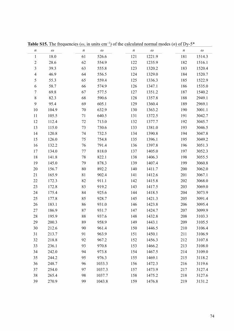
Table S15. The frequencies (ω, in units cm–1) of the calculated normal modes (n) of Dy-5*
n ω n ω n ω n ω
1 18.0 61 526.6 121 1221.9 181 1514.3
2 28.6 62 554.9 122 1235.9 182 1516.1
3 39.3 63 555.8 123 1320.2 183 1520.4
4 46.9 64 556.5 124 1329.0 184 1520.7
5 55.3 65 559.4 125 1336.3 185 1522.9
6 58.7 66 574.9 126 1347.1 186 1535.0
7 69.8 67 577.5 127 1351.2 187 1540.2
8 82.3 68 590.6 128 1357.8 188 2949.1
9 95.4 69 605.1 129 1360.4 189 2969.1
10 104.9 70 632.9 130 1363.2 190 3001.1
11 105.5 71 640.5 131 1372.5 191 3042.7
12 112.4 72 713.0 132 1377.7 192 3045.7
13 115.0 73 730.6 133 1381.0 193 3046.5
14 120.8 74 732.5 134 1390.8 194 3047.8
15 126.0 75 754.8 135 1396.1 195 3049.2
16 132.2 76 791.4 136 1397.8 196 3051.3
17 134.0 77 818.0 137 1405.0 197 3052.3
18 141.8 78 822.1 138 1406.3 198 3055.5
19 145.0 79 878.3 139 1407.4 199 3060.8
20 156.7 80 892.2 140 1411.7 200 3062.0
21 165.9 81 902.4 141 1412.6 201 3067.1
22 172.3 82 911.1 142 1415.8 202 3068.0
23 172.8 83 919.2 143 1417.5 203 3069.0
24 175.4 84 925.6 144 1418.5 204 3073.9
25 177.8 85 928.7 145 1421.3 205 3091.4
26 183.1 86 931.0 146 1423.8 206 3095.4
27 186.9 87 931.7 147 1424.7 207 3099.9
28 195.9 88 937.6 148 1432.8 208 3103.3
29 200.3 89 958.9 149 1443.1 209 3105.5
30 212.6 90 961.4 150 1446.5 210 3106.4
31 213.7 91 963.9 151 1450.1 211 3106.9
32 218.8 92 967.2 152 1456.3 212 3107.8
33 236.1 93 970.8 153 1466.2 213 3108.0
34 242.0 94 973.8 154 1467.5 214 3109.0
35 244.2 95 976.3 155 1469.1 215 3118.2
36 248.7 96 1033.3 156 1472.3 216 3119.6
37 254.0 97 1037.3 157 1473.9 217 3127.4
38 265.4 98 1037.7 158 1475.2 218 3127.6
39 270.9 99 1043.8 159 1476.8 219 3131.2
74
40 272.3 100 1045.0 160 1478.6 220 3131.6
41 276.4 101 1045.3 161 1481.1 221 3133.9
42 279.0 102 1048.4 162 1483.3 222 3135.8
43 280.1 103 1074.8 163 1484.5 223 3137.3
44 288.7 104 1085.3 164 1485.1 224 3138.5
45 292.0 105 1085.8 165 1485.9 225 3141.2
46 294.5 106 1086.7 166 1486.7 226 3141.3
47 302.1 107 1120.6 167 1488.6 227 3141.6
48 308.6 108 1122.6 168 1489.7 228 3151.5
49 317.2 109 1136.4 169 1490.9 229 3151.9
50 338.1 110 1142.6 170 1491.9 230 3153.9
51 350.8 111 1146.9 171 1492.7 231 3155.2
52 356.6 112 1150.3 172 1495.3 232 3155.5
53 373.7 113 1153.7 173 1497.1 233 3160.0
54 394.7 114 1156.6 174 1502.3 234 3162.0
55 409.7 115 1167.6 175 1506.5 235 3173.4
56 440.6 116 1182.9 176 1507.9 236 3182.6
57 458.4 117 1193.6 177 1509.4 237 3188.1
58 465.9 118 1193.7 178 1512.5
59 489.6 119 1196.9 179 1512.7
60 510.7 120 1202.9 180 1514.1
75
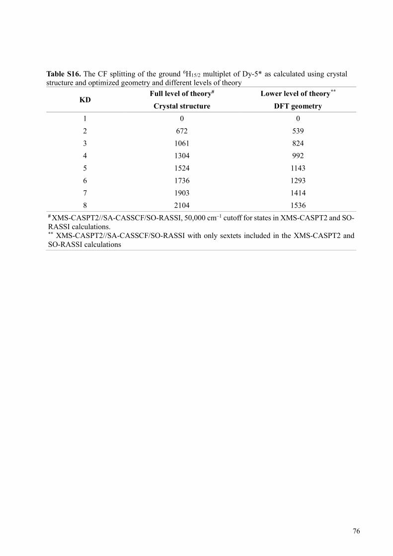
Table S16. The CF splitting of the ground 6H15/2 multiplet of Dy-5* as calculated using crystal structure and optimized geometry and different levels of theory
KD Full level of theory# Lower level of theory**
Crystal structure DFT geometry
1 0 0
2 672 539
3 1061 824
4 1304 992
5 1524 1143
6 1736 1293
7 1903 1414
8 2104 1536
# XMS-CASPT2//SA-CASSCF/SO-RASSI, 50,000 cm–1 cutoff for states in XMS-CASPT2 and SO-RASSI calculations. ** XMS-CASPT2//SA-CASSCF/SO-RASSI with only sextets included in the XMS-CASPT2 and SO-RASSI calculations
76
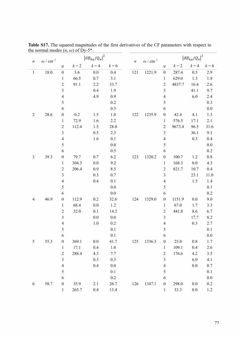
Table S17. The squared magnitudes of the first derivatives of the CF parameters with respect to the normal modes (n, ω) of Dy-5*.
n ω / cm–1 �����/���
�
n ω / cm–1 �����/���
�
q k = 2 k = 4 k = 6 q k = 2 k = 4 k = 6
1 18.0 0 3.6 0.0 0.4 121 1221.9 0 287.4 0.5 2.9
1 66.5 0.7 3.1 1 629.0 1.3 1.8
2 91.1 2.2 33.7 2 4837.7 16.4 2.6
3 0.4 1.9 3 41.1 9.7
4 4.9 0.9 4 6.0 2.4
5 0.2 5 0.3
6 0.3 6 0.0
2 28.6 0 0.2 1.5 1.0 122 1235.9 0 42.4 4.1 1.3
1 72.9 1.6 2.2 1 576.5 17.1 2.1
2 112.4 1.5 28.0 2 9673.8 96.5 31.6
3 0.5 2.3 3 36.1 9.1
4 1.6 0.1 4 0.3 0.4
5 0.0 5 0.0
6 0.5 6 0.2
3 39.3 0 79.7 0.7 6.2 123 1320.2 0 100.7 1.2 0.8
1 304.3 0.0 9.2 1 168.3 0.0 4.3
2 206.4 0.9 8.5 2 821.7 10.7 0.4
3 0.3 0.7 3 23.1 11.0
4 0.4 0.1 4 1.5 1.4
5 0.0 5 0.1
6 0.0 6 0.2
4 46.9 0 112.9 0.2 32.6 124 1329.0 0 1151.9 0.0 9.0
1 68.4 0.0 1.2 1 67.0 1.7 3.3
2 32.0 0.1 14.2 2 441.8 8.6 6.7
3 0.0 0.0 3 17.7 8.2
4 1.0 0.2 4 0.3 2.7
5 0.1 5 0.1
6 0.1 6 0.0
5 55.3 0 369.1 0.0 41.7 125 1336.3 0 25.0 0.8 1.7
1 17.1 0.4 1.0 1 109.1 0.4 2.6
2 288.4 4.3 7.7 2 176.6 4.2 3.5
3 0.3 0.3 3 6.0 4.1
4 0.4 0.0 4 0.0 0.7
5 0.1 5 0.1
6 0.2 6 0.0
6 58.7 0 35.9 2.1 26.7 126 1347.1 0 298.0 0.0 0.2
1 265.7 0.4 13.4 1 33.3 0.0 1.2
77
2 419.1 4.9 1.4 2 683.9 3.5 0.3
3 1.2 0.2 3 2.5 1.2
4 0.2 0.1 4 0.0 0.1
5 0.1 5 0.0
6 0.3 6 0.1
7 69.8 0 438.6 0.1 23.7 127 1351.2 0 0.7 1.1 2.4
1 82.3 0.4 3.3 1 189.5 0.3 1.0
2 14.5 0.3 2.6 2 2098.8 5.4 1.3
3 0.2 0.4 3 6.3 2.7
4 1.7 0.1 4 0.4 0.4
5 0.1 5 0.1
6 0.3 6 0.1
8 82.3 0 3.5 1.2 1.3 128 1357.8 0 380.5 0.7 10.6
1 13.3 0.9 0.0 1 118.1 0.7 0.2
2 20.4 0.1 0.1 2 367.9 1.1 2.4
3 0.1 0.2 3 6.9 3.9
4 0.4 0.0 4 1.0 1.6
5 0.0 5 0.0
6 0.0 6 0.5
9 95.4 0 354.2 15.9 3.1 129 1360.4 0 11.1 0.1 0.2
1 33.7 0.6 5.6 1 103.9 0.7 2.0
2 210.5 0.9 2.0 2 1261.0 9.7 3.9
3 0.2 0.3 3 12.7 6.7
4 2.4 0.6 4 1.9 1.2
5 0.0 5 0.0
6 0.2 6 0.0
10 104.9 0 46.8 3.7 0.6 130 1363.2 0 121.4 0.1 3.6
1 11.9 0.7 1.5 1 50.9 2.5 0.5
2 34.2 3.4 4.5 2 370.2 5.7 8.1
3 0.3 0.1 3 2.2 2.2
4 0.6 0.3 4 0.6 0.7
5 0.0 5 0.1
6 0.2 6 0.2
11 105.5 0 194.3 4.8 25.8 131 1372.5 0 3.7 0.4 3.0
1 0.5 3.7 1.8 1 125.9 5.2 2.1
2 32.7 0.1 2.0 2 121.1 2.8 2.4
3 0.2 0.0 3 5.1 2.6
4 0.8 0.6 4 0.4 0.6
5 0.1 5 0.9
6 0.0 6 0.7
12 112.4 0 36.2 0.1 5.8 132 1377.7 0 329.6 7.2 0.8
78
1 17.3 0.3 0.1 1 42.0 0.6 0.7
2 12.6 0.2 0.2 2 160.8 13.9 11.4
3 0.4 0.6 3 5.7 5.3
4 0.1 0.0 4 0.6 1.7
5 0.0 5 0.0
6 0.0 6 0.0
13 115.0 0 11.4 0.3 21.4 133 1381.0 0 227.6 0.4 4.8
1 9.2 0.6 0.3 1 55.2 3.8 0.1
2 10.6 0.0 1.6 2 171.1 6.6 9.0
3 0.4 0.1 3 8.3 11.8
4 0.2 0.2 4 0.1 2.8
5 0.1 5 0.0
6 0.0 6 0.0
14 120.8 0 107.0 0.2 35.6 134 1390.8 0 324.4 0.0 2.1
1 6.8 0.3 0.7 1 2.5 0.1 1.1
2 114.6 2.3 10.1 2 2.8 2.8 1.2
3 0.2 0.2 3 1.4 0.1
4 1.4 0.1 4 0.8 0.4
5 0.2 5 0.4
6 0.0 6 0.8
15 126.0 0 216.1 17.3 8.9 135 1396.1 0 53.1 0.2 0.8
1 1.9 1.2 5.2 1 11.8 0.2 0.0
2 9.0 0.9 5.3 2 24.9 0.4 0.2
3 0.1 0.3 3 0.2 0.1
4 2.3 0.6 4 0.1 0.2
5 0.1 5 0.0
6 0.4 6 0.0
16 132.2 0 34.7 47.5 55.0 136 1397.8 0 4.1 0.1 0.1
1 24.1 0.0 9.1 1 4.6 0.1 0.1
2 26.0 1.6 13.9 2 52.5 0.0 0.3
3 0.0 2.0 3 0.1 0.0
4 1.3 0.4 4 0.2 0.0
5 0.3 5 0.0
6 0.4 6 0.0
17 134.0 0 1.3 0.4 0.3 137 1405.0 0 11.0 17.1 0.2
1 6.0 3.0 3.0 1 61.5 1.3 0.3
2 27.8 0.4 2.8 2 2382.1 6.5 1.2
3 0.1 0.8 3 7.4 3.7
4 1.2 0.1 4 1.1 0.3
5 0.1 5 0.0
6 0.1 6 0.5
79
18 141.8 0 21.6 0.1 0.3 138 1406.3 0 6.9 30.9 5.4
1 1.8 4.5 2.6 1 86.8 0.0 0.8
2 8.9 0.7 4.9 2 1318.6 13.3 5.5
3 0.8 1.0 3 1.1 0.5
4 0.6 0.0 4 0.0 0.3
5 0.1 5 0.0
6 0.1 6 0.0
19 145.0 0 107.6 5.6 0.1 139 1407.4 0 44.9 0.1 1.1
1 91.9 0.4 2.3 1 171.6 0.1 0.1
2 42.9 0.2 0.8 2 2479.8 0.6 1.2
3 0.3 0.3 3 18.9 6.3
4 0.1 0.1 4 0.2 1.4
5 0.1 5 0.1
6 0.1 6 0.0
20 156.7 0 90.9 10.9 9.4 140 1411.7 0 21.7 0.3 0.9
1 115.1 5.0 3.7 1 0.9 0.2 0.2
2 88.5 4.1 1.6 2 23.0 0.3 0.1
3 1.5 1.9 3 0.1 0.1
4 2.0 0.2 4 0.1 0.0
5 0.4 5 0.0
6 0.0 6 0.0
21 165.9 0 229.8 3.4 36.0 141 1412.6 0 130.4 1.4 0.2
1 254.4 5.4 1.1 1 1.0 0.0 0.5
2 100.8 6.0 4.8 2 53.9 0.4 0.3
3 0.1 2.1 3 0.6 0.4
4 3.2 0.2 4 0.3 0.1
5 0.2 5 0.0
6 0.3 6 0.0
22 172.3 0 163.6 0.2 6.6 142 1415.8 0 17.5 0.0 0.0
1 89.7 3.1 1.5 1 1.0 0.3 0.1
2 123.0 6.1 4.2 2 24.0 0.1 0.3
3 0.1 0.0 3 0.1 0.1
4 2.8 0.4 4 0.0 0.0
5 0.4 5 0.0
6 0.1 6 0.0
23 172.8 0 64.0 12.4 25.6 143 1417.5 0 205.5 10.9 4.9
1 72.9 2.1 2.1 1 2.1 0.0 0.1
2 16.6 3.5 6.0 2 298.9 0.4 1.7
3 0.1 0.4 3 3.7 2.2
4 0.2 0.1 4 0.0 0.1
5 0.2 5 0.1
80
6 0.5 6 0.0
24 175.4 0 447.2 1.3 2.5 144 1418.5 0 18.6 65.9 0.3
1 185.4 5.7 2.4 1 1.0 3.4 0.9
2 61.2 5.3 5.1 2 121.7 2.7 6.0
3 0.7 0.6 3 8.7 4.4
4 1.2 0.5 4 0.2 0.2
5 0.0 5 0.5
6 0.0 6 0.0
25 177.8 0 3.6 0.3 33.9 145 1421.3 0 93.1 0.0 1.0
1 13.4 0.5 0.7 1 35.6 1.7 0.1
2 80.3 0.9 1.4 2 275.0 4.3 3.0
3 0.1 0.1 3 4.7 2.2
4 0.1 0.1 4 0.1 0.7
5 0.2 5 0.0
6 0.0 6 0.0
26 183.1 0 334.3 2.4 0.7 146 1423.8 0 616.6 6.3 0.0
1 268.4 3.3 1.7 1 23.7 1.8 0.5
2 4.1 0.9 1.1 2 25.2 0.6 0.8
3 0.0 0.1 3 0.3 0.4
4 0.7 0.1 4 0.2 0.1
5 0.1 5 0.0
6 0.0 6 0.0
27 186.9 0 100.2 0.1 16.4 147 1424.7 0 42.3 3.2 0.8
1 68.7 1.6 0.7 1 5.0 0.7 0.2
2 20.8 2.1 1.0 2 9.8 1.0 0.7
3 0.0 0.0 3 1.0 0.6
4 0.6 0.8 4 0.4 0.0
5 0.4 5 0.0
6 0.8 6 0.0
28 195.9 0 31.7 0.1 2.2 148 1432.8 0 892.1 21.6 0.7
1 94.4 2.2 0.2 1 3.5 2.3 1.5
2 77.6 0.2 0.8 2 504.2 1.1 3.9
3 0.3 0.2 3 14.7 8.5
4 1.1 0.1 4 1.1 0.2
5 0.1 5 0.4
6 0.1 6 0.0
29 200.3 0 571.7 1.7 50.2 149 1443.1 0 290.8 22.5 21.5
1 591.1 13.1 9.8 1 76.1 6.9 13.5
2 21.0 0.1 1.9 2 400.9 2.3 2.2
3 0.2 0.3 3 9.8 20.3
4 3.1 0.6 4 1.3 11.2
81
5 2.2 5 0.2
6 0.9 6 0.0
30 212.6 0 12.1 0.3 0.3 150 1446.5 0 43.0 10.1 2.1
1 191.8 3.7 0.7 1 859.9 1.8 4.2
2 142.4 1.0 0.3 2 334.6 70.6 74.0
3 0.6 0.0 3 2.6 1.5
4 2.9 0.2 4 3.6 0.7
5 0.1 5 1.3
6 1.7 6 0.1
31 213.7 0 10.9 0.7 0.1 151 1450.1 0 166.1 41.1 0.3
1 271.0 5.4 0.5 1 234.0 0.3 0.8
2 293.8 0.0 1.7 2 3153.0 26.8 16.8
3 0.9 0.8 3 44.6 23.7
4 0.8 0.4 4 7.4 9.9
5 0.4 5 0.8
6 1.3 6 0.2
32 218.8 0 92.4 1.3 0.0 152 1456.3 0 839.1 45.9 0.0
1 64.0 3.0 1.5 1 1282.8 1.5 1.8
2 127.7 1.4 1.7 2 1855.7 31.5 14.9
3 1.9 0.3 3 31.5 28.1
4 7.8 0.2 4 1.6 1.5
5 0.0 5 0.3
6 0.0 6 0.4
33 236.1 0 678.4 28.5 8.7 153 1466.2 0 639.9 90.6 18.4
1 21.2 11.2 10.1 1 73.7 25.1 24.7
2 331.4 5.1 0.0 2 174.1 2.6 5.2
3 2.6 1.4 3 1.9 0.2
4 22.4 2.8 4 1.6 0.7
5 0.4 5 0.2
6 1.9 6 0.0
34 242.0 0 24.7 4.2 0.1 154 1467.5 0 16.0 0.3 0.7
1 15.8 3.1 1.7 1 22.9 3.9 1.0
2 39.9 0.4 0.1 2 206.6 8.2 9.2
3 0.1 0.0 3 0.7 0.2
4 0.5 0.5 4 1.2 0.1
5 0.0 5 0.1
6 0.0 6 0.4
35 244.2 0 3.1 0.2 0.6 155 1469.1 0 46.7 3.1 0.0
1 33.1 0.1 0.6 1 123.1 1.7 1.3
2 13.9 1.2 0.3 2 192.0 1.5 0.0
3 0.4 0.4 3 0.4 0.5
82
4 1.0 0.1 4 5.4 0.4
5 0.1 5 0.0
6 0.4 6 0.2
36 248.7 0 88.5 0.1 0.1 156 1472.3 0 0.8 25.2 9.3
1 162.2 4.6 0.1 1 62.1 6.3 1.9
2 38.3 0.1 0.1 2 49.6 3.6 1.4
3 1.1 0.8 3 0.3 0.8
4 2.6 0.0 4 1.0 0.1
5 0.0 5 0.0
6 0.0 6 0.0
37 254.0 0 82.4 0.4 0.2 157 1473.9 0 876.5 10.3 14.2
1 4.8 0.5 1.1 1 28.5 4.4 0.7
2 219.2 1.5 0.5 2 2687.9 1.2 4.2
3 0.1 0.7 3 0.8 0.7
4 1.0 0.6 4 1.8 0.0
5 0.3 5 0.1
6 2.7 6 0.8
38 265.4 0 41.2 7.7 1.4 158 1475.2 0 100.9 19.0 1.1
1 40.0 0.7 2.6 1 41.3 4.2 1.5
2 144.8 3.3 1.2 2 1422.8 2.2 0.3
3 0.1 1.1 3 4.8 3.1
4 0.3 0.2 4 2.3 0.3
5 0.0 5 0.0
6 0.6 6 1.0
39 270.9 0 5.4 0.2 5.8 159 1476.8 0 139.7 0.0 0.0
1 42.8 1.0 0.4 1 77.1 9.0 0.7
2 62.7 1.9 0.9 2 1091.1 10.4 2.4
3 0.3 0.2 3 0.9 0.2
4 4.3 0.2 4 12.8 0.4
5 0.2 5 0.1
6 1.1 6 1.3
40 272.3 0 14.6 0.4 0.3 160 1478.6 0 348.4 0.1 6.7
1 24.3 3.5 0.5 1 12.1 0.8 1.1
2 41.3 6.8 1.8 2 86.2 3.3 0.3
3 0.3 1.3 3 2.3 1.3
4 4.9 1.2 4 2.7 0.5
5 0.3 5 0.1
6 1.2 6 0.1
41 276.4 0 1.3 0.0 0.6 161 1481.1 0 157.9 1.0 1.5
1 79.5 2.8 10.0 1 13.9 1.4 1.5
2 3.5 2.4 5.5 2 754.8 0.7 2.2
83
3 0.3 0.5 3 0.1 0.0
4 0.3 0.1 4 2.0 0.0
5 0.0 5 0.1
6 0.0 6 0.7
42 279.0 0 11.0 2.7 16.9 162 1483.3 0 2.0 0.1 0.0
1 105.8 0.7 5.3 1 80.5 1.2 0.5
2 45.5 11.4 0.1 2 133.5 0.9 0.0
3 0.8 1.0 3 0.0 0.1
4 1.2 0.2 4 4.8 0.3
5 0.2 5 0.0
6 0.4 6 0.3
43 280.1 0 18.6 0.4 7.6 163 1484.5 0 12.9 0.2 5.0
1 25.2 13.6 0.5 1 11.8 1.9 0.7
2 156.0 42.5 4.0 2 148.1 2.5 0.0
3 1.2 6.7 3 2.0 1.3
4 1.9 0.6 4 0.4 0.1
5 1.1 5 0.0
6 1.9 6 0.0
44 288.7 0 30.1 2.5 3.4 164 1485.1 0 49.8 1.1 0.5
1 10.3 1.1 0.2 1 58.8 4.2 1.5
2 144.1 3.5 0.3 2 1278.9 0.6 0.2
3 0.2 1.4 3 5.7 3.6
4 0.5 0.2 4 1.7 0.2
5 0.7 5 0.1
6 6.6 6 0.4
45 292.0 0 6.2 0.2 5.8 165 1485.9 0 10.9 0.6 4.6
1 60.5 0.1 1.0 1 24.3 0.4 0.4
2 213.1 0.3 0.9 2 15.3 0.5 0.0
3 2.9 2.4 3 1.3 0.5
4 0.2 0.1 4 0.4 0.0
5 0.1 5 0.0
6 0.1 6 0.0
46 294.5 0 48.3 3.4 15.1 166 1486.7 0 126.1 0.1 0.3
1 3.7 1.9 0.5 1 133.3 3.8 4.2
2 213.3 4.8 2.2 2 112.2 4.0 2.3
3 1.3 1.2 3 0.1 0.2
4 0.1 0.3 4 6.7 0.5
5 0.0 5 0.0
6 0.8 6 0.5
47 302.1 0 120.4 0.0 0.4 167 1488.6 0 338.5 1.2 0.6
1 13.4 1.7 0.1 1 15.5 1.0 0.6
84
2 164.6 3.5 0.3 2 124.0 1.1 0.3
3 2.9 1.9 3 0.2 0.2
4 2.3 0.0 4 0.6 0.0
5 0.1 5 0.0
6 0.2 6 0.2
48 308.6 0 0.2 2.9 2.6 168 1489.7 0 326.4 2.3 1.1
1 36.2 0.8 0.0 1 83.4 0.6 1.9
2 15.9 1.9 0.1 2 429.9 1.0 3.0
3 0.4 0.1 3 0.6 0.6
4 4.2 0.1 4 7.6 0.4
5 0.1 5 0.2
6 1.6 6 1.7
49 317.2 0 17.7 0.4 7.4 169 1490.9 0 142.0 1.4 4.9
1 1.0 0.1 0.4 1 11.9 1.0 0.1
2 23.1 2.9 1.5 2 93.1 1.1 0.2
3 1.8 0.8 3 1.2 0.6
4 8.9 2.3 4 2.9 0.2
5 0.7 5 0.1
6 1.2 6 0.1
50 338.1 0 3994.8 89.6 146.1 170 1491.9 0 364.8 2.9 8.2
1 55.6 102.6 182.0 1 99.1 0.9 1.3
2 71.6 22.4 13.2 2 1044.9 1.7 1.9
3 2.7 3.5 3 1.8 0.6
4 1.3 70.6 4 1.7 0.0
5 165.9 5 0.1
6 42.0 6 1.4
51 350.8 0 96.1 1.5 13.8 171 1492.7 0 1.1 0.5 0.0
1 98.9 13.5 4.4 1 248.8 6.2 3.5
2 995.2 4.1 3.0 2 405.1 2.7 0.3
3 9.7 5.2 3 1.6 1.1
4 11.5 4.1 4 2.0 0.1
5 3.0 5 0.0
6 18.6 6 0.1
52 356.6 0 44.5 1.7 4.9 172 1495.3 0 106.8 10.1 0.0
1 15.1 0.9 2.2 1 58.2 3.4 2.1
2 306.2 1.7 6.2 2 249.8 0.7 0.7
3 5.5 3.1 3 2.1 1.1
4 22.8 1.4 4 0.5 0.1
5 5.0 5 0.1
6 14.0 6 0.2
53 373.7 0 12.2 1.7 5.4 173 1497.1 0 5.7 8.1 0.2
85
1 24.2 3.9 1.9 1 17.3 1.8 1.5
2 56.5 0.9 2.3 2 266.0 0.2 0.3
3 1.4 0.4 3 0.6 0.5
4 2.1 1.6 4 4.6 0.0
5 0.1 5 0.0
6 3.2 6 0.5
54 394.7 0 1.1 13.0 14.6 174 1502.3 0 56.0 0.3 5.6
1 20100.1 37.6 10.1 1 28.8 0.7 0.5
2 2238.1 3.4 40.8 2 24.7 3.1 0.2
3 14.6 14.0 3 0.8 0.5
4 64.4 4.4 4 1.0 0.1
5 0.3 5 0.0
6 0.1 6 0.0
55 409.7 0 4942.4 16.6 63.8 175 1506.5 0 506.5 4.8 0.1
1 21268.8 18.8 5.8 1 30.1 0.8 0.2
2 4249.5 37.4 6.7 2 132.4 0.4 0.0
3 26.3 27.3 3 2.4 0.5
4 21.0 2.9 4 1.7 0.7
5 2.1 5 0.0
6 0.4 6 0.0
56 440.6 0 59.0 5.9 18.3 176 1507.9 0 105.3 0.1 2.5
1 32.9 1.1 2.0 1 27.5 2.7 0.8
2 88.4 0.6 0.3 2 318.1 3.7 0.4
3 1.0 0.6 3 1.9 0.9
4 0.4 0.7 4 1.7 0.2
5 0.1 5 0.0
6 0.4 6 0.2
57 458.4 0 74.3 5.4 5.9 177 1509.4 0 0.6 3.0 5.4
1 44.4 0.7 2.9 1 5.9 0.2 0.1
2 85.3 0.3 0.5 2 1.2 6.7 1.0
3 0.8 0.7 3 1.3 0.6
4 1.0 1.2 4 1.0 1.3
5 0.0 5 0.1
6 0.1 6 0.3
58 465.9 0 75.2 0.1 2.9 178 1512.5 0 5.2 0.4 2.0
1 130.7 2.4 0.1 1 124.7 2.2 2.5
2 230.2 0.5 0.2 2 2108.9 3.3 3.4
3 0.2 1.2 3 9.7 4.9
4 1.3 1.0 4 6.2 1.1
5 0.1 5 0.1
6 0.4 6 0.2
86
59 489.6 0 505.0 4.6 1.3 179 1512.7 0 459.7 1.3 0.2
1 216.4 2.1 11.9 1 10.4 0.2 0.0
2 501.1 5.5 3.5 2 183.5 1.8 1.2
3 0.6 0.8 3 3.8 2.9
4 0.4 2.5 4 2.2 0.3
5 0.2 5 0.1
6 0.4 6 0.2
60 510.7 0 1785.8 6.2 19.9 180 1514.1 0 113.3 0.1 2.0
1 357.7 15.0 59.8 1 22.8 0.6 0.5
2 231.4 1.1 1.6 2 1755.1 12.3 9.4
3 3.9 4.0 3 12.9 8.4
4 0.8 2.7 4 0.6 3.3
5 5.1 5 0.3
6 2.2 6 0.0
61 526.6 0 1572.7 7.4 17.6 181 1514.3 0 0.6 22.0 0.6
1 839.9 6.4 28.6 1 163.4 0.5 0.0
2 309.8 4.0 12.5 2 1790.3 20.9 9.4
3 8.5 3.1 3 23.1 18.4
4 4.5 1.4 4 2.5 3.5
5 1.6 5 0.0
6 1.1 6 0.1
62 554.9 0 16.2 0.4 0.0 182 1516.1 0 7.2 2.4 0.0
1 78.1 0.4 7.0 1 78.6 0.5 1.0
2 8212.0 52.7 30.4 2 683.5 0.5 1.0
3 16.4 2.5 3 0.2 0.2
4 0.2 0.0 4 0.3 0.0
5 0.0 5 0.0
6 0.0 6 1.3
63 555.8 0 84.2 44.6 2.9 183 1520.4 0 6.7 1.5 3.4
1 262.7 1.3 2.9 1 38.9 1.0 0.6
2 5208.5 7.4 1.6 2 933.0 0.1 0.3
3 7.8 14.5 3 3.2 1.2
4 0.2 4.6 4 2.2 0.2
5 0.4 5 0.0
6 0.0 6 0.2
64 556.5 0 11.9 0.0 3.0 184 1520.7 0 4.0 0.1 0.2
1 28.3 0.3 0.2 1 22.2 1.1 0.9
2 35.5 0.9 0.7 2 118.7 0.1 0.6
3 0.3 0.1 3 3.5 1.9
4 0.3 0.4 4 1.5 0.0
5 0.4 5 0.1
87
6 0.1 6 0.3
65 559.4 0 39.0 38.0 5.8 185 1522.9 0 4892.0 6.8 3.9
1 786.7 1.3 15.1 1 598.9 43.8 3.1
2 488.2 4.5 3.1 2 7620.4 2.2 13.0
3 4.1 3.8 3 34.7 1.2
4 17.2 5.1 4 40.2 4.1
5 0.3 5 0.3
6 0.3 6 7.2
66 574.9 0 19.3 0.7 0.1 186 1535.0 0 3.6 0.0 0.2
1 1212.1 13.8 0.1 1 387.5 155.4 25.9
2 370.6 0.8 10.4 2 103.5 25.0 4.8
3 16.6 6.5 3 0.2 11.0
4 14.1 1.7 4 0.3 6.1
5 0.3 5 2.0
6 0.8 6 0.1
67 577.5 0 2.1 2.7 15.4 187 1540.2 0 495.5 45.2 6.7
1 14825.0 79.7 0.0 1 46.1 62.3 9.1
2 2826.1 50.7 52.9 2 716.7 21.5 7.9
3 4.0 19.4 3 4.9 3.5
4 33.5 1.9 4 0.4 10.2
5 0.0 5 1.8
6 0.9 6 0.2
68 590.6 0 53.4 1.0 244.7 188 2949.1 0 107.5 6.1 0.0
1 8648.9 160.7 44.8 1 50.8 2.6 0.0
2 4028.4 159.2 15.0 2 259.7 0.4 0.5
3 123.7 73.0 3 4.3 0.8
4 50.3 11.2 4 2.5 0.3
5 0.8 5 0.1
6 0.3 6 3.2
69 605.1 0 3682.0 17.4 0.3 189 2969.1 0 463.9 2.2 0.7
1 516.8 9.9 0.1 1 35.9 0.5 0.6
2 417.2 4.7 3.7 2 1177.2 0.3 1.5
3 7.1 3.8 3 0.0 0.1
4 4.1 4.1 4 2.5 0.2
5 0.4 5 0.2
6 0.9 6 1.7
70 632.9 0 80.3 14.4 6.8 190 3001.1 0 1282.5 0.8 0.1
1 4136.8 24.7 15.1 1 34.2 0.5 0.3
2 1779.2 277.8 10.9 2 45.3 3.3 0.2
3 333.5 58.2 3 0.2 0.1
4 363.6 161.6 4 0.7 0.1
88
5 63.3 5 0.0
6 16.4 6 0.0
71 640.5 0 655.8 388.3 12.4 191 3042.7 0 19.6 0.0 6.8
1 1466.0 283.5 50.5 1 8.6 0.5 0.3
2 7103.1 1422.6 403.2 2 101.9 2.1 0.3
3 207.1 260.5 3 1.4 0.2
4 120.1 50.2 4 1.6 0.2
5 8.7 5 0.2
6 0.1 6 0.3
72 713.0 0 0.3 2.8 0.8 192 3045.7 0 2.0 0.0 1.4
1 35.1 0.1 21.4 1 45.2 0.2 0.1
2 638.6 17.1 5.9 2 77.8 3.5 0.8
3 1.5 3.4 3 0.1 0.1
4 2.1 1.2 4 3.4 0.0
5 0.2 5 0.0
6 0.0 6 0.6
73 730.6 0 757.1 32.8 0.2 193 3046.5 0 53.7 0.0 1.8
1 1486.5 59.6 20.8 1 25.8 0.3 0.1
2 5071.8 64.3 1.3 2 13.1 2.0 0.4
3 181.2 78.0 3 0.0 0.0
4 24.2 39.9 4 1.6 0.0
5 2.5 5 0.0
6 0.1 6 0.1
74 732.5 0 511.1 40.5 13.9 194 3047.8 0 0.0 0.0 0.9
1 384.0 9.0 2.0 1 9.7 0.0 0.0
2 2308.7 69.3 3.0 2 63.9 0.6 0.1
3 180.8 95.8 3 0.0 0.0
4 39.5 54.0 4 0.2 0.0
5 11.0 5 0.0
6 0.7 6 0.0
75 754.8 0 127.8 645.8 218.7 195 3049.2 0 34.1 0.0 2.5
1 13776.4 3316.7 759.2 1 23.1 0.1 0.1
2 1669.6 1024.4 1817.2 2 16.3 0.3 0.1
3 675.0 1579.2 3 0.1 0.1
4 997.5 864.1 4 0.3 0.0
5 120.2 5 0.0
6 7.7 6 0.0
76 791.4 0 3.4 3.8 35.9 196 3051.3 0 13.5 0.0 0.0
1 111.6 2.9 4.2 1 6.2 0.1 0.2
2 397.5 4.7 6.5 2 74.7 2.3 0.3
3 2.2 2.1 3 0.0 0.1
89
4 3.7 0.2 4 0.1 0.0
5 0.1 5 0.0
6 0.0 6 0.0
77 818.0 0 524.7 24.8 6.4 197 3052.3 0 1.1 0.0 0.3
1 518.9 3.4 1.0 1 14.2 0.0 0.1
2 128.1 0.9 3.7 2 3.0 0.3 0.0
3 4.9 1.2 3 0.0 0.0
4 20.5 0.1 4 0.2 0.0
5 0.1 5 0.0
6 0.0 6 0.0
78 822.1 0 23.2 0.3 0.0 198 3055.5 0 9.8 1.0 1.7
1 934.0 6.1 1.4 1 3.9 1.3 0.0
2 19.1 2.1 2.5 2 4.8 0.3 0.2
3 0.6 0.2 3 0.1 0.0
4 24.3 1.0 4 0.1 0.1
5 0.4 5 0.0
6 0.1 6 0.0
79 878.3 0 23.0 0.3 0.1 199 3060.8 0 11.2 0.3 0.2
1 7.5 3.0 0.2 1 2.5 0.0 0.1
2 1850.8 7.7 1.1 2 16.8 0.1 0.2
3 0.5 0.1 3 0.1 0.1
4 0.8 0.2 4 0.0 0.0
5 0.8 5 0.0
6 0.7 6 0.0
80 892.2 0 10.2 1.0 0.2 200 3062.0 0 4.2 0.1 0.4
1 25.2 2.7 0.6 1 0.6 0.1 0.0
2 965.6 0.9 0.6 2 27.1 0.1 0.4
3 5.2 0.8 3 0.2 0.1
4 1.1 0.0 4 0.0 0.0
5 0.1 5 0.0
6 0.0 6 0.0
81 902.4 0 35.9 2.6 1.0 201 3067.1 0 0.9 0.0 0.2
1 14.1 0.1 0.2 1 0.5 0.0 0.0
2 225.6 0.3 0.1 2 18.7 0.0 0.0
3 0.0 0.0 3 0.0 0.1
4 1.5 0.1 4 0.0 0.0
5 0.0 5 0.0
6 0.1 6 0.0
82 911.1 0 6.1 0.0 0.0 202 3068.0 0 1.9 0.0 0.0
1 67.3 0.2 0.0 1 0.4 0.1 0.0
2 482.3 3.4 0.2 2 8.2 0.0 0.1
90
3 1.1 0.0 3 0.0 0.0
4 0.7 0.0 4 0.1 0.0
5 0.3 5 0.0
6 0.2 6 0.0
83 919.2 0 1.2 0.0 0.1 203 3069.0 0 1.9 0.0 0.0
1 8.8 0.1 0.2 1 1.9 0.0 0.1
2 4.3 0.2 0.0 2 12.2 0.0 0.0
3 0.0 0.1 3 0.1 0.1
4 0.2 0.0 4 0.0 0.0
5 0.1 5 0.0
6 0.0 6 0.0
84 925.6 0 19.4 0.0 0.0 204 3073.9 0 4.9 0.0 0.0
1 19.6 0.7 0.1 1 9.6 0.3 0.1
2 95.5 1.1 0.2 2 19.8 0.0 0.2
3 0.4 0.1 3 0.1 0.2
4 0.1 0.0 4 0.0 0.0
5 0.0 5 0.0
6 0.0 6 0.0
85 928.7 0 1.7 2.6 2.0 205 3091.4 0 0.3 0.0 0.0
1 36.3 0.6 0.1 1 3.4 0.0 0.0
2 29.2 0.5 0.2 2 221.9 0.7 0.0
3 0.0 0.1 3 0.1 0.1
4 3.8 0.1 4 0.1 0.0
5 0.1 5 0.0
6 0.1 6 0.5
86 931.0 0 2.0 0.0 0.1 206 3095.4 0 5.5 0.0 0.0
1 23.6 0.3 0.0 1 10.7 1.8 0.0
2 40.0 0.1 0.2 2 158.2 0.9 0.4
3 0.1 0.1 3 0.1 0.1
4 1.0 0.1 4 2.2 0.2
5 0.0 5 0.0
6 0.0 6 0.3
87 931.7 0 4.1 0.7 0.5 207 3099.9 0 9.6 0.1 0.2
1 32.0 0.1 0.3 1 2.9 0.1 0.0
2 223.8 0.2 0.1 2 7.8 0.0 0.1
3 1.6 0.5 3 0.1 0.0
4 0.4 0.5 4 0.0 0.0
5 0.0 5 0.0
6 0.0 6 0.0
88 937.6 0 33.4 0.5 0.1 208 3103.3 0 28.8 0.0 0.0
1 9.3 0.3 0.3 1 0.5 0.1 0.0
91
2 12.9 0.1 0.1 2 31.5 0.3 0.0
3 0.4 0.2 3 0.0 0.0
4 0.4 0.1 4 0.3 0.0
5 0.0 5 0.0
6 0.0 6 0.0
89 958.9 0 347.5 6.3 0.2 209 3105.5 0 151.6 0.1 1.0
1 239.8 0.2 1.5 1 37.3 2.5 0.0
2 1723.4 3.9 0.1 2 24.0 0.9 1.6
3 0.3 0.4 3 0.2 0.0
4 1.0 0.1 4 0.5 0.0
5 0.9 5 0.0
6 1.9 6 0.0
90 961.4 0 0.3 48.8 0.5 210 3106.4 0 11.5 1.0 2.3
1 190.1 5.2 1.8 1 38.3 1.8 0.0
2 3337.8 76.8 22.8 2 52.9 1.8 0.9
3 42.6 22.5 3 0.4 0.0
4 0.2 3.0 4 0.2 0.0
5 0.1 5 0.0
6 0.0 6 0.0
91 963.9 0 5.0 0.1 0.1 211 3106.9 0 70.4 2.6 0.0
1 12.5 1.1 0.2 1 3.3 0.7 0.1
2 82.4 5.0 1.0 2 1.3 0.1 0.1
3 0.5 0.0 3 0.7 0.2
4 0.9 0.0 4 1.0 0.6
5 0.1 5 0.1
6 0.6 6 0.2
92 967.2 0 18.6 0.3 1.1 212 3107.8 0 29.9 1.1 2.5
1 61.5 0.0 0.0 1 6.7 0.2 0.0
2 2243.5 1.2 3.6 2 11.8 0.2 0.1
3 40.7 16.4 3 0.1 0.0
4 1.9 4.6 4 0.0 0.0
5 0.3 5 0.0
6 0.0 6 0.0
93 970.8 0 21.7 0.1 0.7 213 3108.0 0 93.9 0.0 2.2
1 42.0 0.1 0.1 1 6.3 0.4 0.4
2 14.3 0.2 0.0 2 10.0 0.0 0.8
3 0.1 0.2 3 0.1 0.2
4 0.7 0.0 4 0.3 0.1
5 0.0 5 0.0
6 0.0 6 0.0
94 973.8 0 21.2 0.4 0.0 214 3109.0 0 18.1 0.1 4.9
92
1 3.1 0.1 0.0 1 3.3 0.7 0.0
2 79.3 0.1 0.1 2 6.0 0.0 0.7
3 2.0 1.6 3 0.1 0.1
4 0.1 0.3 4 0.1 0.1
5 0.0 5 0.0
6 0.0 6 0.0
95 976.3 0 70.0 0.3 0.0 215 3118.2 0 1.6 0.9 2.4
1 47.1 0.2 0.2 1 1.0 0.0 0.1
2 16.9 0.7 0.2 2 15.8 0.2 0.2
3 0.9 0.7 3 0.1 0.0
4 0.7 0.1 4 0.0 0.0
5 0.0 5 0.0
6 0.0 6 0.0
96 1033.3 0 20.9 0.0 0.1 216 3119.6 0 50.2 0.9 0.1
1 2252.6 19.6 23.4 1 41.0 0.3 0.2
2 500.7 1.3 9.8 2 40.8 1.4 0.1
3 1.5 1.1 3 0.2 0.2
4 22.0 1.0 4 1.3 0.1
5 0.3 5 0.0
6 0.0 6 0.3
97 1037.3 0 20.7 8.1 12.7 217 3127.4 0 1.4 0.0 0.0
1 1426.8 5.8 4.5 1 13.4 0.1 0.0
2 5691.1 61.9 16.0 2 0.5 0.1 0.0
3 24.3 10.7 3 0.1 0.0
4 9.4 2.7 4 0.1 0.0
5 0.1 5 0.0
6 0.2 6 0.0
98 1037.7 0 1132.4 10.7 32.8 218 3127.6 0 39.6 0.0 0.2
1 810.1 11.9 1.4 1 4.3 0.2 0.0
2 1441.6 9.1 10.5 2 22.1 0.1 0.1
3 5.7 6.1 3 0.0 0.0
4 16.5 0.3 4 0.1 0.0
5 0.1 5 0.0
6 0.0 6 0.0
99 1043.8 0 516.3 20.4 4.5 219 3131.2 0 22.3 0.4 0.1
1 26.1 8.5 0.8 1 15.8 0.2 0.0
2 333.9 74.1 27.7 2 3.7 0.4 0.1
3 4.0 3.8 3 0.0 0.0
4 0.5 4.1 4 0.0 0.0
5 1.2 5 0.0
6 0.1 6 0.0
93
100 1045.0 0 152.9 11.7 1.2 220 3131.6 0 11.8 0.3 0.4
1 213.9 3.4 0.8 1 1.5 0.1 0.0
2 9431.5 59.1 10.2 2 44.9 0.3 0.1
3 122.5 58.0 3 0.0 0.1
4 1.2 0.9 4 0.1 0.0
5 0.7 5 0.0
6 0.3 6 0.0
101 1045.3 0 286.2 0.6 1.2 221 3133.9 0 24.6 0.0 0.2
1 48.1 3.2 1.5 1 6.1 0.0 0.1
2 271.1 14.2 3.3 2 8.9 0.3 0.1
3 69.2 40.4 3 0.1 0.1
4 1.8 6.3 4 0.0 0.0
5 1.1 5 0.0
6 0.2 6 0.0
102 1048.4 0 454.3 0.0 3.8 222 3135.8 0 8.1 0.1 0.2
1 18.8 1.6 4.4 1 1.2 0.0 0.0
2 375.2 37.4 4.1 2 2.0 0.2 0.0
3 25.0 15.6 3 0.0 0.0
4 1.8 3.7 4 0.0 0.0
5 0.1 5 0.0
6 0.1 6 0.0
103 1074.8 0 6.1 0.0 0.0 223 3137.3 0 69.7 0.1 0.0
1 46.8 3.6 0.2 1 2.6 0.0 0.1
2 633.4 15.4 3.1 2 3.9 0.1 0.0
3 2.7 1.7 3 0.1 0.1
4 0.8 0.8 4 0.0 0.0
5 0.1 5 0.0
6 0.2 6 0.0
104 1085.3 0 10.5 2.8 1.3 224 3138.5 0 125.4 0.1 0.2
1 14.6 1.1 0.3 1 26.1 3.5 0.3
2 132.1 3.8 2.8 2 87.4 0.5 0.4
3 0.9 0.7 3 0.1 0.1
4 0.2 0.1 4 0.1 0.0
5 0.0 5 0.0
6 0.0 6 0.0
105 1085.8 0 7.5 0.0 1.2 225 3141.2 0 0.0 0.0 3.5
1 303.6 0.7 15.5 1 3.9 0.1 0.1
2 33.5 0.9 4.7 2 53.3 0.2 0.2
3 1.8 1.8 3 0.3 0.0
4 5.6 1.4 4 0.2 0.0
5 0.2 5 0.0
94
6 0.1 6 0.0
106 1086.7 0 8.5 0.7 37.9 226 3141.3 0 42.5 0.9 2.4
1 173.4 0.2 9.3 1 0.5 0.0 0.1
2 37.4 1.2 6.1 2 31.9 0.3 0.2
3 0.0 0.4 3 0.0 0.0
4 3.5 1.0 4 0.1 0.0
5 0.3 5 0.0
6 0.0 6 0.0
107 1120.6 0 2.8 0.0 0.0 227 3141.6 0 0.0 0.2 0.1
1 2.6 0.2 0.0 1 0.3 0.0 0.0
2 18.1 0.4 0.5 2 0.9 0.0 0.0
3 0.2 0.0 3 0.0 0.0
4 0.1 0.2 4 0.0 0.0
5 0.1 5 0.0
6 0.0 6 0.0
108 1122.6 0 161.0 0.3 9.8 228 3151.5 0 14.4 0.1 3.7
1 12.3 4.1 1.8 1 3.2 0.1 0.1
2 1028.0 0.7 0.3 2 1.1 0.1 0.0
3 6.7 5.2 3 0.1 0.0
4 0.2 1.1 4 0.1 0.0
5 0.1 5 0.0
6 0.1 6 0.0
109 1136.4 0 2021.8 25.1 2.4 229 3151.9 0 1.3 0.0 0.3
1 1269.6 9.5 0.8 1 0.1 0.0 0.0
2 4745.4 6.3 0.5 2 11.7 0.0 0.0
3 5.7 0.5 3 0.0 0.0
4 2.6 0.1 4 0.1 0.0
5 0.8 5 0.0
6 0.5 6 0.0
110 1142.6 0 186.6 3.8 18.9 230 3153.9 0 13.7 0.9 1.4
1 96.7 7.8 4.8 1 3.4 0.2 0.0
2 2747.1 0.6 0.4 2 42.5 0.3 0.0
3 13.8 2.4 3 0.0 0.1
4 0.1 0.3 4 0.1 0.1
5 0.1 5 0.0
6 0.0 6 0.2
111 1146.9 0 1765.4 1.3 1.7 231 3155.2 0 25.7 0.0 0.1
1 1123.6 5.7 0.7 1 0.3 0.0 0.0
2 3012.1 2.4 2.0 2 34.3 0.6 0.0
3 20.0 2.6 3 0.0 0.0
4 0.3 0.6 4 0.3 0.0
95
5 0.1 5 0.0
6 0.2 6 0.0
112 1150.3 0 27.7 1.1 0.0 232 3155.5 0 10.3 0.0 0.1
1 129.3 0.8 1.8 1 0.2 0.0 0.0
2 191.7 1.2 0.7 2 9.1 0.2 0.0
3 3.1 1.3 3 0.0 0.0
4 0.8 0.1 4 0.1 0.0
5 0.0 5 0.0
6 0.0 6 0.1
113 1153.7 0 1016.1 1.0 1.4 233 3160.0 0 27.9 1.0 1.4
1 239.9 2.1 2.6 1 4.0 0.1 0.0
2 323.2 0.4 2.1 2 0.4 0.0 0.0
3 1.7 0.3 3 0.1 0.1
4 0.2 0.1 4 0.1 0.0
5 0.0 5 0.0
6 0.0 6 0.0
114 1156.6 0 751.8 2.1 8.4 234 3162.0 0 2.8 0.0 0.0
1 64.6 0.1 2.8 1 0.3 0.0 0.0
2 112.6 1.1 0.1 2 5.4 0.1 0.0
3 1.8 1.6 3 0.0 0.0
4 0.0 0.3 4 0.2 0.0
5 0.0 5 0.0
6 0.0 6 0.0
115 1167.6 0 90.9 0.8 3.2 235 3173.4 0 4.0 0.0 0.1
1 36.9 0.6 0.1 1 0.1 0.0 0.0
2 3116.9 5.8 1.0 2 21.5 0.1 0.0
3 0.5 0.3 3 0.1 0.0
4 0.3 0.3 4 0.1 0.0
5 0.0 5 0.0
6 0.0 6 0.0
116 1182.9 0 480.0 2.6 2.0 236 3182.6 0 1.5 0.0 0.1
1 34.0 4.5 2.0 1 1.4 0.0 0.0
2 535.7 0.1 0.6 2 8.2 0.1 0.0
3 3.4 3.0 3 0.0 0.0
4 0.5 1.5 4 0.1 0.0
5 0.0 5 0.0
6 0.1 6 0.0
117 1193.6 0 1196.2 104.0 8.0 237 3188.1 0 3.8 0.0 0.1
1 7428.8 91.5 38.7 1 0.9 0.0 0.0
2 3196.4 48.6 65.8 2 2.6 0.0 0.0
3 42.6 6.1 3 0.0 0.0
96
4 1.1 1.2 4 0.0 0.0
5 0.0 5 0.0
6 0.1 6 0.0
118 1193.7 0 44.4 0.5 0.4
1 256.0 55.4 11.7
2 10944.8 72.3 16.9
3 136.4 65.3
4 2.9 15.3
5 1.9
6 0.1
119 1196.9 0 292.9 3.4 0.1
1 102.0 0.5 0.9
2 62.1 4.8 1.9
3 1.6 0.5
4 7.2 0.6
5 0.0
6 0.2
120 1202.9 0 186.9 5.4 2.9
1 224.8 6.0 0.3
2 323.1 7.4 1.1
3 1.3 0.7
4 4.0 0.3
5 0.2
6 0.2
97
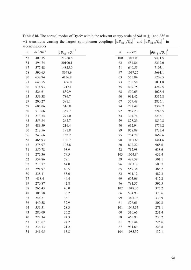
Table S18. The normal modes of Dy-5* within the relevant energy scale of Δ� = ±1 and Δ� =
±2 transitions causing the largest spin-phonon couplings ����±�/���� and ����±�/���
� in
ascending order
n ω / cm–1 ����±�/���� n ω / cm–1 ����±�/���
�
55 409.75 21268.8 100 1045.03 9431.5
54 394.74 20100.1 62 554.86 8212.0
67 577.48 14825.0 71 640.55 7103.1
68 590.65 8648.9 97 1037.26 5691.1
70 632.94 4136.8 63 555.84 5208.5
71 640.55 1466.0 73 730.58 5071.8
66 574.93 1212.1 55 409.75 4249.5
61 526.61 839.9 68 590.65 4028.4
65 559.38 786.7 90 961.42 3337.8
29 200.27 591.1 67 577.48 2826.1
69 605.06 516.8 74 732.48 2308.7
60 510.66 357.7 92 967.23 2243.5
31 213.74 271.0 54 394.74 2238.1
63 555.84 262.7 79 878.29 1850.8
59 489.59 216.4 70 632.94 1779.2
30 212.56 191.8 89 958.89 1723.4
36 248.66 162.2 75 754.78 1669.6
58 465.93 130.7 98 1037.68 1441.6
42 278.97 105.8 80 892.22 965.6
51 350.78 98.9 72 712.98 638.6
41 276.36 79.5 103 1074.84 633.4
62 554.86 78.1 59 489.59 501.1
32 218.77 64.0 96 1033.33 500.7
45 291.97 60.5 65 559.38 488.2
50 338.11 55.6 82 911.12 482.3
57 458.4 44.4 69 605.06 417.2
39 270.87 42.8 76 791.37 397.5
38 265.43 40.0 102 1048.36 375.2
48 308.58 36.2 66 574.93 370.6
35 244.21 33.1 99 1043.76 333.9
56 440.58 32.9 61 526.61 309.8
64 556.51 28.3 101 1045.33 271.1
43 280.09 25.2 60 510.66 231.4
40 272.34 24.3 58 465.93 230.2
53 373.67 24.2 81 902.44 225.6
33 236.13 21.2 87 931.69 223.8
34 241.95 15.8 104 1085.32 132.1
98
52 356.62 15.1 77 818.01 128.1
47 302.13 13.4 84 925.63 95.5
44 288.7 10.3 56 440.58 88.4
37 253.99 4.8 57 458.4 85.3
46 294.5 3.7 91 963.9 82.4
49 317.2 1.0 94 973.81 79.3
86 930.97 40.0
106 1086.74 37.4
64 556.51 35.5
105 1085.82 33.5
85 928.75 29.2
78 822.12 19.1
95 976.3 16.9
93 970.78 14.3
88 937.64 12.9
83 919.22 4.3
99
Captions for Movies S1 to S7: Movie S1. Normal vibrational mode 54. Movie S2. Normal vibrational mode 55. Movie S3. Normal vibrational mode 66. Movie S4. Normal vibrational mode 67. Movie S5. Normal vibrational mode 68. Movie S6. Normal vibrational mode 70. Movie S7. Normal vibrational mode 71. Captions for Data S1: Caption 1: Cartesian coordinates for the optimized geometry of Dy-5*. Caption 2: Cartesian coordinates for the displacement geometries used in the evaluation of the spin-phonon couplings in Dy-5*. Caption 3: Original data for the magnetic property measurements.
100
References and Notes 1. N. Ishikawa, M. Sugita, T. Ishikawa, S. Y. Koshihara, Y. Kaizu, Lanthanide double-decker
complexes functioning as magnets at the single-molecular level. J. Am. Chem. Soc. 125, 8694–8695 (2003). doi:10.1021/ja029629n Medline
2. B. M. Day, F.-S. Guo, R. A. Layfield, Cyclopentadienyl ligands in lanthanide single-molecule magnets: One ring to rule them all? Acc. Chem. Res. 51, 1880–1889 (2018). doi:10.1021/acs.accounts.8b00270 Medline
3. J.-L. Liu, Y.-C. Chen, M.-L. Tong, Symmetry strategies for high performance lanthanide-based single-molecule magnets. Chem. Soc. Rev. 47, 2431–2453 (2018). doi:10.1039/C7CS00266A Medline
4. J. M. Frost, K. L. M. Harriman, M. Murugesu, The rise of 3-d single-ion magnets in molecular magnetism: Towards materials from molecules? Chem. Sci. 7, 2470–2491 (2016). doi:10.1039/C5SC03224E Medline
5. M. Shiddiq, D. Komijani, Y. Duan, A. Gaita-Ariño, E. Coronado, S. Hill, Enhancing coherence in molecular spin qubits via atomic clock transitions. Nature 531, 348–351 (2016). doi:10.1038/nature16984 Medline
6. S. Thiele, F. Balestro, R. Ballou, S. Klyatskaya, M. Ruben, W. Wernsdorfer, Electrically driven nuclear spin resonance in single-molecule magnets. Science 344, 1135–1138 (2014). doi:10.1126/science.1249802 Medline
7. D. N. Woodruff, R. E. P. Winpenny, R. A. Layfield, Lanthanide single-molecule magnets. Chem. Rev. 113, 5110–5148 (2013). doi:10.1021/cr400018q Medline
8. P. Zhang, L. Zhang, J. Tang, Lanthanide single molecule magnets: Progress and perspective. Dalton Trans. 44, 3923–3929 (2015). doi:10.1039/C4DT03329A Medline
9. J. D. Rinehart, M. Fang, W. J. Evans, J. R. Long, A N23− radical-bridged terbium complex
exhibiting magnetic hysteresis at 14 K. J. Am. Chem. Soc. 133, 14236–14239 (2011). doi:10.1021/ja206286h Medline
10. Y.-C. Chen, J.-L. Liu, L. Ungur, J. Liu, Q.-W. Li, L.-F. Wang, Z.-P. Ni, L. F. Chibotaru, X.-M. Chen, M.-L. Tong, Symmetry-supported magnetic blocking at 20 K in pentagonal bipyramidal Dy(III) single-ion magnets. J. Am. Chem. Soc. 138, 2829–2837 (2016). doi:10.1021/jacs.5b13584 Medline
11. S. K. Gupta, T. Rajeshkumar, G. Rajaraman, R. Murugavel, An air-stable Dy(III) single-ion magnet with high anisotropy barrier and blocking temperature. Chem. Sci. 7, 5181–5191 (2016). doi:10.1039/C6SC00279J Medline
12. F. Liu, D. S. Krylov, L. Spree, S. M. Avdoshenko, N. A. Samoylova, M. Rosenkranz, A. Kostanyan, T. Greber, A. U. B. Wolter, B. Büchner, A. A. Popov, Single molecule magnet with an unpaired electron trapped between two lanthanide ions inside a fullerene. Nat. Commun. 8, 16098 (2017). doi:10.1038/ncomms16098 Medline
13. F.-S. Guo, B. M. Day, Y.-C. Chen, M.-L. Tong, A. Mansikkamäki, R. A. Layfield, A dysprosium metallocene single-molecule magnet functioning at the axial limit. Angew. Chem. Int. Ed. 56, 11445–11449 (2017). doi:10.1002/anie.201705426 Medline
101
14. C. A. P. Goodwin, F. Ortu, D. Reta, N. F. Chilton, D. P. Mills, Molecular magnetic hysteresis at 60 kelvin in dysprosocenium. Nature 548, 439–442 (2017). doi:10.1038/nature23447 Medline
15. C. A. P. Goodwin, D. Reta, F. Ortu, N. F. Chilton, D. P. Mills, Synthesis and electronic structures of heavy lanthanide metallocenium cations. J. Am. Chem. Soc. 139, 18714–18724 (2017). doi:10.1021/jacs.7b11535 Medline
16. S. J. Connelly, W. Kaminsky, D. M. Heinekey, Structure and solution reactivity of (triethylsilylium)triethylsilane cations. Organometallics 32, 7478–7481 (2013). doi:10.1021/om400970j
17. C. Benelli, D. Gatteschi, Introduction to Molecular Magnetism: From Transition Metals to Lanthanides (Wiley-VCH, 2015).
18. Y.-N. Guo, G.-F. Xu, Y. Guo, J. Tang, Relaxation dynamics of dysprosium(III) single molecule magnets. Dalton Trans. 40, 9953–9963 (2011). doi:10.1039/c1dt10474h Medline
19. S. Demir, M. I. Gonzalez, L. E. Darago, W. J. Evans, J. R. Long, Giant coercivity and high magnetic blocking temperatures for N2
3− radical-bridged dilanthanide complexes upon ligand dissociation. Nat. Commun. 8, 2144 (2017). doi:10.1038/s41467-017-01553-w Medline
20. L. Ungur, L. F. Chibotaru, Strategies toward high-temperature lanthanide-based single-molecule magnets. Inorg. Chem. 55, 10043–10056 (2016). doi:10.1021/acs.inorgchem.6b01353 Medline
21. L. Ungur, J. J. Le Roy, I. Korobkov, M. Murugesu, L. F. Chibotaru, Fine-tuning the local symmetry to attain record blocking temperature and magnetic remanence in a single-ion magnet. Angew. Chem. Int. Ed. 53, 4413–4417 (2014). doi:10.1002/anie.201310451 Medline
22. J. J. Le Roy, L. Ungur, I. Korobkov, L. F. Chibotaru, M. Murugesu, Coupling strategies to enhance single-molecule magnet properties of erbium-cyclooctatetraenyl complexes. J. Am. Chem. Soc. 136, 8003–8010 (2014). doi:10.1021/ja5022552 Medline
23. J. J. Le Roy, M. Jeletic, S. I. Gorelsky, I. Korobkov, L. Ungur, L. F. Chibotaru, M. Murugesu, An organometallic building block approach to produce a multidecker 4f single-molecule magnet. J. Am. Chem. Soc. 135, 3502–3510 (2013). doi:10.1021/ja310642h Medline
24. K. L. M. Harriman, J. J. Le Roy, L. Ungur, R. J. Holmberg, I. Korobkov, M. Murugesu, Cycloheptatrienyl trianion: An elusive bridge in the search of exchange coupled dinuclear organolanthanide single-molecule magnets. Chem. Sci. 8, 231–240 (2017). doi:10.1039/C6SC01224H Medline
25. T. P. Latendresse, N. S. Bhuvanesh, M. Nippe, Hard single-molecule magnet behavior by a linear trinuclear lanthanide–[1]metallocenophane complex. J. Am. Chem. Soc. 139, 14877–14880 (2017). doi:10.1021/jacs.7b08690 Medline
102
26. T. Pugh, N. F. Chilton, R. A. Layfield, A low-symmetry dysprosium metallocene single-molecule magnet with a high anisotropy barrier. Angew. Chem. Int. Ed. 55, 11082–11085 (2016). doi:10.1002/anie.201604346 Medline
27. T. Pugh, F. Tuna, L. Ungur, D. Collison, E. J. L. McInnes, L. F. Chibotaru, R. A. Layfield, Influencing the properties of dysprosium single-molecule magnets with phosphorus donor ligands. Nat. Commun. 6, 7492 (2015). doi:10.1038/ncomms8492 Medline
28. T. Pugh, V. Vieru, L. F. Chibotaru, R. A. Layfield, Magneto-structural correlations in arsenic- and selenium-ligated dysprosium single-molecule magnets. Chem. Sci. 7, 2128–2137 (2016). doi:10.1039/C5SC03755G Medline
29. T. Pugh, N. F. Chilton, R. A. Layfield, Antimony-ligated dysprosium single-molecule magnets as catalysts for stibine dehydrocoupling. Chem. Sci. 8, 2073–2080 (2017). doi:10.1039/C6SC04465D Medline
30. A. F. R. Kilpatrick, F.-S. Guo, B. M. Day, A. Mansikkamäki, R. A. Layfield, F. G. N. Cloke, Single-molecule magnet properties of a monometallic dysprosium pentalene complex. Chem. Commun. (Camb.) 54, 7085–7088 (2018). doi:10.1039/C8CC03516D Medline
31. L. Ungur, L. F. Chibotaru, Computational Modelling of Magnetic Properties of Lanthanide Compounds in Lanthanide and Actinides in Molecular Magnetism, R. A. Layfield, M. Murugesu, Eds. (Wiley-VCH, 2015).
32. T. Shiozaki, W. Gyõrffy, P. Celani, H.-J. Werner, Communication: extended multi-state complete active space second-order perturbation theory: energy and nuclear gradients. J. Chem. Phys. 135, 081106 (2011). doi:10.1063/1.3633329 Medline
33. L. Ungur, L. F. Chibotaru, Ab initio crystal field for lanthanides. Chemistry 23, 3708–3718 (2017). doi:10.1002/chem.201605102 Medline
34. L. F. Chibotaru, in Ab Initio Methodology for Pseudospin Hamiltonians of Anisotropic Magnetic Complexes, S. A. Rice, A. R. Dinner, Eds. (Advances in Chemical Physics Series, Wiley, 2013), vol. 153, pp. 397–519.
35. L. Ungur, M. Thewissen, J.-P. Costes, W. Wernsdorfer, L. F. Chibotaru, Interplay of strongly anisotropic metal ions in magnetic blocking of complexes. Inorg. Chem. 52, 6328–6337 (2013). doi:10.1021/ic302568x Medline
36. K. R. McClain, C. A. Gould, K. Chakarawet, S. J. Teat, T. J. Groshens, J. R. Long, B. G. Harvey, High-temperature magnetic blocking and magneto-structural correlations in a series of dysprosium(III) metallocenium single-molecule magnets. Chem. Sci. (Camb.) 9, 8492–8503 (2018). doi:10.1039/C8SC03907K
37. H. Sitzmann, Synthese von 1,2,3,4,5-Pentaisopropylcyclopentadien und 1,3,5-Tri-tert-butylcyclopentadien / Synthesis of 1,2,3,4,5-Pentaisopropylcyclopentadiene and 1,3,5-Tri-tert-butylcyclopentadiene. Z. Naturforsch B 44, 1293–1297 (1989). doi:10.1515/znb-1989-1025
38. S. M. Cendrowski-Guillaume, G. Le Gland, M. Nierlich, M. Ephritikhine, Lanthanide borohydrides as precursors to organometallic compounds. mono(cyclooctatetraenyl) neodymium complexes. Organometallics 19, 5654–5660 (2000). doi:10.1021/om000558f
103
39. W. J. Evans, S. A. Kozimor, J. W. Ziller, N. Kaltsoyannis, Structure, reactivity, and density functional theory analysis of the six-electron reductant, [(C5Me5)2U]2(μ-η6:η6-C6H6), synthesized via a new mode of (C5Me5)3M reactivity. J. Am. Chem. Soc. 126, 14533–14547 (2004). doi:10.1021/ja0463886 Medline
40. O. V. Dolomanov, L. J. Bourhis, R. J. Gildea, J. A. K. Howard, H. Puschmann, OLEX2: A complete structure solution, refinement and analysis program. J. Appl. Cryst. 42, 339–341 (2009). doi:10.1107/S0021889808042726
41. G. M. Sheldrick, SHELXT—Integrated space-group and crystal-structure determination. Acta Crystallogr. A Found Adv. 71, 3–8 (2015). doi:10.1107/S2053273314026370 Medline
42. G. M. Sheldrick, Crystal structure refinement with SHELXL. Acta Crystallogr. C Struct. Chem. 71, 3–8 (2015). doi:10.1107/S2053229614024218 Medline
43. G. A. Bain, J. F. Berry, Diamagnetic corrections and Pascal’s constants. J. Chem. Educ. 85, 532 (2008). doi:10.1021/ed085p532
44. D. Gatteschi, R. Sessoli, J. Villain, Molecular Nanomagnets (Oxford Univ. Press, 2006). 45. D. Gatteschi, R. Sessoli, Quantum tunneling of magnetization and related phenomena in
molecular materials. Angew. Chem. Int. Ed. 42, 268–297 (2003). doi:10.1002/anie.200390099 Medline
46. F. Aquilante, J. Autschbach, R. K. Carlson, L. F. Chibotaru, M. G. Delcey, L. De Vico, I. Fdez Galván, N. Ferré, L. M. Frutos, L. Gagliardi, M. Garavelli, A. Giussani, C. E. Hoyer, G. Li Manni, H. Lischka, D. Ma, P. Å. Malmqvist, T. Müller, A. Nenov, M. Olivucci, T. B. Pedersen, D. Peng, F. Plasser, B. Pritchard, M. Reiher, I. Rivalta, I. Schapiro, J. Segarra-Martí, M. Stenrup, D. G. Truhlar, L. Ungur, A. Valentini, S. Vancoillie, V. Veryazov, V. P. Vysotskiy, O. Weingart, F. Zapata, R. Lindh, Molcas 8: New capabilities for multiconfigurational quantum chemical calculations across the periodic table. J. Comput. Chem. 37, 506–541 (2016). doi:10.1002/jcc.24221 Medline
47. P.-O. Widmark, P.-Å. Malmqvist, B. O. Roos, Density matrix averaged atomic natural orbital (ANO) basis sets for correlated molecular wave functions. Theor. Chim. Acta 77, 291–306 (1990). doi:10.1007/BF01120130
48. B. O. Roos, R. Lindh, P. Å. Malmqvist, V. Veryazov, P.-O. Widmark, Main group atoms and dimers studied with a new relativistic ANO basis set. J. Phys. Chem. A 108, 2851–2858 (2004). doi:10.1021/jp031064+
49. W. Kutzelnigg, W. Liu, Quasirelativistic theory equivalent to fully relativistic theory. J. Chem. Phys. 123, 241102 (2005). doi:10.1063/1.2137315 Medline
50. M. Filatov, Comment on “Quasirelativistic theory equivalent to fully relativistic theory” [J. Chem. Phys. 123, 241102 (2005)]. J. Chem. Phys. 125, 107101 (2006). doi:10.1063/1.2338033 Medline
51. D. Peng, M. Reiher, Exact decoupling of the relativistic Fock operator. Theor. Chem. Acc. 131, 1081 (2012). doi:10.1007/s00214-011-1081-y
52. B. O. Roos, in Ab Initio Methods in Quantum Chemistry, Part II, K. P. Lawley, Ed. (Advances in Chemical Physics Series, Wiley, 1987), vol. 69, pp. 399–455.
104
53. P. Siegbahn, A. Heiberg, B. Roos, B. Levy, A comparison of the super-CI and the Newton-Raphson scheme in the complete active space SCF method. Phys. Scr. 21, 323–327 (1980). doi:10.1088/0031-8949/21/3-4/014
54. B. O. Roos, P. R. Taylor, P. E. M. Sigbahn, A complete active space SCF method (CASSCF) using a density matrix formulated super-CI approach. Chem. Phys. 48, 157–173 (1980). doi:10.1016/0301-0104(80)80045-0
55. P. E. M. Siegbahn, J. Almlöf, A. Heiberg, B. Roos, The complete active space SCF (CASSCF) method in a Newton–Raphson formulation with application to the HNO molecule. J. Chem. Phys. 74, 2384–2396 (1981). doi:10.1063/1.441359
56. B. O. Roos, R. Lindh, P. Å. Malmqvist, V. Veryazov, P.-O. Widmark, Multiconfigurational Quantum Chemistry (Wiley, 2016).
57. B. O. Roos, P. Linse, P. E. M. Siegbahn, M. R. A. Blomberg, A simple method for the evaluation of the second-order-perturbation energy from external double-excitations with a CASSCF reference wavefunction. Chem. Phys. 66, 197–207 (1982). doi:10.1016/0301-0104(82)88019-1
58. K. Andersson, P. Å. Malmqvist, B. O. Roos, A. J. Sadlej, K. Wolinski, Second-order perturbation theory with a CASSCF reference function. J. Phys. Chem. 94, 5483–5488 (1990). doi:10.1021/j100377a012
59. K. Andersson, P.-Å. Malmqvist, B. O. Roos, Second‐order perturbation theory with a complete active space self‐consistent field reference function. J. Chem. Phys. 96, 1218–1226 (1992). doi:10.1063/1.462209
60. P. Å. Malmqvist, B. O. Roos, B. Schimmelpfennig, The restricted active space (RAS) state interaction approach with spin–orbit coupling. Chem. Phys. Lett. 357, 230–240 (2002). doi:10.1016/S0009-2614(02)00498-0
61. L. F. Chibotaru, L. Ungur, Ab initio calculation of anisotropic magnetic properties of complexes. I. Unique definition of pseudospin Hamiltonians and their derivation. J. Chem. Phys. 137, 064112 (2012). doi:10.1063/1.4739763 Medline
62. M. J. Frisch, G. W. Trucks, H. B. Schlegel, G. E. Scuseria, M. A. Robb, J. R. Cheeseman, G. Scalmani, V. Barone, G. A. Petersson, H. Nakatsuji, X. Li, M. Caricato, A. Marenich, J. Bloino, B. G. Janesko, R. Gomperts, B. Mennucci, H. P. Hratchian, J. V. Ortiz, A. F. Izmaylov, J. L. Sonnenberg, D. Williams-Young, F. Ding, F. Lipparini, F. Egidi, J. Goings, B. Peng, A. Petrone, T. Henderson, D. Ranasinghe, V. G. Zakrzewski, J. Gao, N. Rega, G. Zheng, W. Liang, M. Hada, M. Ehara, K. Toyota, R. Fukuda, J. Hasegawa, M. Ishida, T. Nakajima, Y. Honda, O. Kitao, H. Nakai, T. Vreven, K. Throssell, J. A. Montgomery Jr., J. E. Peralta, F. Ogliaro, M. Bearpark, J. J. Heyd, E. Brothers, K. N. Kudin, V. N. Staroverov, T. Keith, R. Kobayashi, J. Normand, K. Raghavachari, A. Rendell, J. C. Burant, S. S. Iyengar, J. Tomasi, M. Cossi, J. M. Millam, M. Klene, C. Adamo, R. Cammi, J. W. Ochterski, R. L. Martin, K. Morokuma, O. Farkas, J. B. Foresman, D. J. Fox, Gaussian 09, Revision D.01 (Gaussian, Inc., Wallingford, CT, 2009).
63. J. P. Perdew, K. Burke, M. Ernzerhof, Generalized gradient approximation made simple. Phys. Rev. Lett. 77, 3865–3868 (1996). doi:10.1103/PhysRevLett.77.3865 Medline
105
64. J. P. Perdew, K. Burke, M. Ernzerhof, Generalized gradient approximation made simple [Phys. Rev. Lett. 77, 3865 (1996)]. Phys. Rev. Lett. 78, 1396 (1997). doi:10.1103/PhysRevLett.78.1396
65. M. Ernzerhof, G. E. Scuseria, Assessment of the Perdew–Burke–Ernzerhof exchange-correlation functional. J. Chem. Phys. 110, 5029–5036 (1999). doi:10.1063/1.478401
66. C. Adamo, V. Barone, Toward reliable density functional methods without adjustable parameters: The PBE0 model. J. Chem. Phys. 110, 6158–6170 (1999). doi:10.1063/1.478522
67. A. Schäfer, C. Huber, R. Ahlrichs, Fully optimized contracted Gaussian basis sets of triple zeta valence quality for atoms Li to Kr. J. Chem. Phys. 100, 5829–5835 (1994). doi:10.1063/1.467146
68. M. Dolg, H. Stoll, A. Savin, H. Preuss, Energy-adjusted pseudopotentials for the rare earth elements. Theor. Chim. Acta 75, 173–194 (1989). doi:10.1007/BF00528565
69. M. Dolg, H. Stoll, H. Preuss, A combination of quasirelativistic pseudopotential and ligand field calculations for lanthanoid compounds. Theor. Chim. Acta 85, 441–450 (1993). doi:10.1007/BF01112983
70. J. Yang, M. Dolg, Valence basis sets for lanthanide 4f-in-core pseudopotentials adapted for crystal orbital ab initio calculations. Theor. Chem. Acc. 113, 212–224 (2005). doi:10.1007/s00214-005-0629-0
71. A. Weigand, X. Cao, J. Yang, M. Dolg, Quasirelativistic f-in-core pseudopotentials and core-polarization potentials for trivalent actinides and lanthanides: Molecular test for trifluorides. Theor. Chem. Acc. 126, 117–127 (2010). doi:10.1007/s00214-009-0584-2
72. S. Grimme, J. Antony, S. Ehrlich, H. Krieg, A consistent and accurate ab initio parametrization of density functional dispersion correction (DFT-D) for the 94 elements H-Pu. J. Chem. Phys. 132, 154104 (2010). doi:10.1063/1.3382344 Medline
73. S. Grimme, S. Ehrlich, L. Goerigk, Effect of the damping function in dispersion corrected density functional theory. J. Comput. Chem. 32, 1456–1465 (2011). doi:10.1002/jcc.21759 Medline
74. N. Iwahara, L. F. Chibotaru, Exchange interaction between J multiplets. Phys. Rev. B 91, 174438 (2015). doi:10.1103/PhysRevB.91.174438
75. N. Iwahara, L. Ungur, L. F. Chibotaru, J ̃-pseudospin states and the crystal field of cubic systems. Phys. Rev. B 98, 054436 (2018). doi:10.1103/PhysRevB.98.054436
76. K. N. Shrivastava, Theory of spin–lattice relaxation. Phys. Status Solidi, B Basic Res. 117, 437–458 (1983). doi:10.1002/pssb.2221170202
77. D. H. Moseley, S. E. Stavretis, K. Thirunavukkuarasu, M. Ozerov, Y. Cheng, L. L. Daemen, J. Ludwig, Z. Lu, D. Smirnov, C. M. Brown, A. Pandey, A. J. Ramirez-Cuesta, A. C. Lamb, M. Atanasov, E. Bill, F. Neese, Z.-L. Xue, Spin-phonon couplings in transition metal complexes with slow magnetic relaxation. Nat. Commun. 9, 2572 (2018). doi:10.1038/s41467-018-04896-0 Medline
106