1

1

2

3

Supplementary Materials for 4

5

Summer Declines in Activity and Body Temperature Offer Polar Bears Limited Energy 6

Savings 7

J.P. Whiteman, H.J. Harlow, G.M. Durner, R. Anderson-Sprecher, S.E. Albeke, E.V. 8

Regehr, S.C. Amstrup, M. Ben-David. 9

10

correspondence to: jwhitema@uwyo.edu 11

12

13

This PDF file includes: 14 15

Materials and Methods 16

Supplementary Text 17

Figs. S1 to S5 18

Tables S1 to S7 19

20

2

Materials and Methods 21

Captures 22

Helicopter captures were performed in 2008 (August, October), 2009 (April–May, 23

August, October), and 2010 (April–May). We searched for bears along the coast, on 24

barrier islands, and up to 150 km offshore on sea ice (when present) between Barrow, 25

Alaska (71°N, 157°W) and the Alaska-Yukon Territory border (69°N, 141°W). In 26

October 2009 we also captured bears on sea ice between 70–79°N and 132–170°W, from 27

the US Coast Guard Cutter Polar Sea. We immobilized bears with a mixture of tiletamine 28

hydrochloride and zolazepam hydrochloride (Telazol; Warner-Lambert Co., Morris 29

Plains, NJ) at estimated doses of 6 mg/kg of body mass, delivered in projectile syringes 30

fired from a dart gun (33). During immobilization and processing we monitored rectal 31

temperature and respiration rate. We weighed bears by suspending them in a net from a 32

digital load scale hoisted from a tripod. Age was determined by counting cementum 33

annuli in extracted vestigial premolars (34). Procedures for capturing, sampling, and 34

instrumenting bears were approved by institutional animal care and use committees at the 35

University of Wyoming and US Geological Survey (USGS) Alaska Science Center, and 36

permitted by the US Fish and Wildlife Service (USFWS; Permit #MA690038). Use of 37

trade names is for descriptive purposes only and does not imply endorsement by the US 38

Government. This research was funded in part by the US Environmental Protection 39

Agency (EPA) but because it was not reviewed by the EPA, no official endorsement 40

should be inferred. 41

42

Location transmitters and collar data 43

Bears were instrumented in April–May (2009) and August (2008, 2009) and 44

recaptured in October or the following spring. At recapture, instrumentation (see below) 45

was retrieved and animals were released. Bears received one of four possible telemetry 46

transmitters, either attached to collars (models TGW-3680 or TGW-4689H; Telonics, 47

Mesa, AZ) or glued to the fur (SPOT or MK-10; Wildlife Computers, Redmond, WA). 48

Collars automatically released 3–7 months after deployment and transmitters attached to 49

fur detached during the molt or earlier. Collars recorded locations with Global 50

Positioning System (GPS) technology (hourly; estimated error < 31 m; 35) or Doppler 51

technology (typically every two days; estimated error: < 400 m, class 3; 401–1000 m, 52

class 2; 1001–2499 m, class 1; 36). Glue-on transmitters were Doppler only. Limits to 53

Argos satellite downloads yielded incomplete location datasets (36). Complete records 54

were obtained from GPS collars retrieved from recaptured bears (n = 17). 55

Both collar models were equipped with a temperature sensor (measurements every 56

30 or 60 minutes, resolution 1°C). TGW-4689H also included an internal accelerometer, 57

sensitive to motion in 3 planes, which recorded the total number of seconds of activity 58

during the previous thirty minutes, every half hour. To 16 collars we attached an external 59

accelerometer (Actiwatch; Mini-Mitter Respironics, Bend, OR) sensitive to motion in all 60

planes, which recorded an acceleration score (a unitless index of acceleration intensity) 61

every 2 minutes (37). 62

63

Temperature logger data 64

3

For recording abdominal temperature we used iButton (DS1922L, hourly 65

measurements, resolution 0.0625°C; Maxim Integrated, San Jose, CA) loggers coated 66

with impermeable paraffin wax and attached to a loop of sterile suture (0 gauge, non-67

dissolvable). Loggers were implanted into five bears fitted with location transmitters and 68

activity loggers, and five bears with transmitters only. We shaved an area 10 × 6 cm on 69

the ventral midline of each bear, approximately 80% of the distance from the xiphoid 70

process to the umbilicus. We injected 1 mL of xylocaine into subcutaneous tissue 71

throughout the shaved region, scrubbed the skin and surrounding fur with povidone-72

iodine. We then used sterile surgical tools to make a 7 cm incision through skin and 73

subcutaneous adipose tissue to expose the linea alba. We made a 5 cm incision through 74

the linea alba, pushed the logger through the incision and off to the side, and secured the 75

logger to the underside of the linea alba, adjacent to the peritoneum, with a single stitch 76

using the loop of suture. We closed the linea alba with interrupted single stitches, the 77

adipose tissue with continuous stitches (00 gauge suture), and the skin with interrupted 78

cruciate or mattress stitches. We used identical surgical procedures when recovering the 79

loggers from recaptured bears. 80

Abdominal temperatures closely reflect intraperitoneal, or “core” temperature. In 81

previous studies, measurements of abdominal temperature of polar bears (recorded from 82

loggers in the same anatomical location as in our study; 38, 39) were nearly identical to 83

intraperitoneal temperatures of polar bears in other studies (22, 40). The peritoneum itself 84

tends to be very thin (< 1 mm in humans; 41) and offers little insulation. 85

To record rump temperature, we used Tidbit V2 loggers (measurements every 5 or 86

10 minutes, resolution 0.02°C; Onset Computer Corporation, Bourne, MA) coated with 87

wax and attached to a loop of sterile suture. Loggers were implanted in seven bears 88

instrumented with transmitters and activity loggers. As described in Durner et al. (6), we 89

made an incision through the skin approximately 15 cm to one side and 5 cm ventral of 90

the base of the bear’s tail. We separated the subcutaneous adipose tissue and secured the 91

logger to the surface of the gluteus maximus muscle using the loop of suture. Loggers 92

were recovered using identical procedures. 93

After abdominal and rump loggers were retrieved, we placed them in a temperature-94

controlled chamber (CL-740A; Omega Engineering Inc., Stamford, CT) and created 4–5 95

point calibration curves for the range of temperatures recorded from each bear. Next, we 96

left loggers in an environmental chamber (Conviron, Pembina, ND) held at a steady 97

temperature for eight weeks and confirmed that measurements did not drift over time. 98

99

Calculating smoothed body temperatures 100

We created smoothed values of abdominal and rump temperatures using seasonal 101

trend decomposition with the “stl” (seasonal trend loess) command in the base statistical 102

package in Program R (54). The seasonal window was periodic and the loess window 103

was 25% of the average sample size of bear records extending from May to October. 104

105

Comparing data from bears on shore and ice 106

To ensure capture effects and incision healing did not influence results, for all 107

analyses we censored all data collected within 120 hours (5 days) after capture, 108

encompassing the period during which polar bears return to regular movement patterns 109

(42, 43), and within 1 hour prior to recapture. Data of movement rate, acceleration scores, 110

4

collar temperature, rump temperature, and body mass for bear 20741, which engaged in a 111

nine-day swim in August–September 2008, were previously reported in a companion 112

study (30). Such a reported long-distance swim is unique (13) thus we excluded these 113

data from calculations and statistical tests of mean movement rate and activity (Fig. 2 and 114

table S1). However, we used these data in models to identify the variables that predicted 115

acceleration scores (table S3) and to evaluate the relationship between acceleration scores 116

and body temperatures (table S5). 117

To assess activity trends over time, we calculated a single activity variable: the 118

proportion of time spent active. To derive this proportion from measurements of the 119

number of seconds of activity per 30 minutes, we divided the count by 1800. For 120

acceleration scores, we first converted the scores to the number of seconds of activity per 121

30 minutes. To achieve this conversion, we calculated a mean acceleration score in half-122

hour blocks. Next, we pooled data for seven bears which had both types of activity 123

measurements and regressed the number of seconds of activity during the previous half 124

hour against the mean acceleration score for that half-hour (total pooled measurements, n 125

= 27,579). The relationship appeared linear for small values but increasingly non-linear at 126

high values, thus we used automated segmented regression (44) and identified a mean 127

acceleration score of 1128 as the breakpoint between linear segments (fig. S4A). For 128

scores below this value, the two types of activity data were related by this equation: 129

130

N = number of seconds of activity over the previous half-hour 131

M = mean acceleration score over the previous half-hour 132

N = (M×0.838) + 38.645 133

134

All monthly means of 30-minute mean acceleration scores were < 1128, thus we 135

used the above equation to convert these data into monthly means of the number of 136

seconds of activity over the previous half-hour. For bears with both types of activity data, 137

the monthly means of the proportion of time spent active based on measured seconds of 138

activity were similar to the monthly means of the proportion of time spent active based 139

on acceleration scores converted to seconds of activity (n = 30, pooled data from seven 140

bears; fig. S4B). This indicates the converted data adequately represents the time spent 141

active. 142

We calculated monthly means of the time spent active (after pooling measured and 143

converted data), movement rate, and smoothed abdominal temperature for each bear, for 144

each month in which it had ≥ 96 hours of measurements. Each monthly mean was 145

categorized as “Shore” or “Ice” based on GPS and Doppler (class 2 and 3) locations. 146

Three bears with location and activity data moved between habitats in July–October, and 147

we calculated a monthly mean for both Shore and Ice accordingly. We compared Shore 148

and Ice monthly means where n ≥ 3 for each group, using the Welch t-test (45). 149

150

Modeling influence of environmental variables on activity 151

We used ARIMA (autoregressive, integrated, moving average) approaches (“arima” 152

command, base statistical package in Program R; 46) to model the influence of three 153

environmental predictor variables on both types of activity data: daily mean of the 154

number of seconds of activity per half-hour, and daily mean of the acceleration scores. 155

Individual models were built for each bear. 156

5

The first model (ARIMA structure [1,0,1]) was built with the predictor “Whale” 157

(only applied to bear locations on shore), a variable between 0–1, describing the daily 158

proportion of hourly GPS locations < 500 m from the site of a whale carcass, ≤ 60 days 159

after the landing of a whale at that site (47, 48). Although bears may scavenge on these 160

carcasses year-round (49), they likely consume the majority of tissue shortly after whales 161

are landed (50). 162

In the second model (ARIMA structure [1,0,1]) we used the predictor “Air 163

Temperature” (only applied to locations on shore), a daily mean of hourly air 164

temperatures recorded < 200 km from each bear location at Alaskan weather stations in 165

Kaktovik, Deadhorse, or Barrow (www.weatherspark.com). 166

In the third model (ARIMA structure [1,0,1]) we used the predictor “Shelf” (only 167

applied to locations on the sea ice), a binary variable indicating whether the daily mean 168

bathymetry value of bear locations was ≥ 300 m. Shelf edges are abrupt in this region of 169

the Arctic and habitat studies indicate that bears select for shallow waters (51, 52). Water 170

depths at bear locations were assigned based on the International Chart of the Arctic 171

Ocean 3.0 (53). 172

173

Correlating activity and body temperatures 174

Abdominal temperature was recorded hourly and rump temperature every 5 or 10 175

minutes, but neither was synchronized with the hourly measurement of other variables 176

(e.g., seconds of activity in the previous half-hour). Thus, for correlating temperatures 177

with activity, we used linear interpolation to estimate body temperatures at the exact time 178

activity was measured. 179

We evaluated the correlation between activity and body temperatures using 180

seemingly-unrelated-time-series models, with commands in the “dlm” (dynamic linear 181

models) package in Program R (55, 56). Models were developed, by bear, with two 182

activity variables matched with interpolated values of the two body temperature variables 183

(abdominal and rump temperature) at an hourly scale. Activity included: a) seconds of 184

activity in the previous half hour, and b) mean acceleration score over the previous half 185

hour. 186

For these models we used adjusted abdominal and rump temperatures, which only 187

included interpolated values within 4 SD of the smoothed temperature; this excluded 188

most outliers of cold temperatures recorded during swimming events (described below). 189

The initial models correlating both measures of activity to rump temperature were 190

unstable and could not provide inferences, likely because rump temperature declined 191

substantially during some periods of inactivity. Thus, we censored the data to only 192

include rump temperature measured when the mean acceleration score during the 193

previous half-hour was ≥ 30. We used mean acceleration scores because all bears with 194

rump temperature measurements had these data, but not all had measurements of number 195

of seconds of activity. We selected this cutoff (≥ 30) after inspecting the data and 196

observing periods of several hours where scores were mostly 0, indicating motionless 197

bears, but which were interrupted by occasional large acceleration scores (e.g. up to 100), 198

likely representing resting interspersed with small movements such as grooming. We 199

reasoned that half-hour means of scores recorded during resting were unlikely to exceed 200

30. Pooled half-hour means of acceleration scores from all bears ranged from 0–4933, 201

with a grand mean (95% CI) across all bears of 454 ± 6. 202

6

203

Cold abdominal and rump temperatures during inactivity and swimming 204

We identified periods of inactivity as ≥ 2 hours with mean hourly movement rate < 205

0.01 m/s and mean acceleration scores < 30, and during these periods we counted the 206

instances of hourly, interpolated abdominal and rump temperatures that were < 35.0°C. 207

We used interpolated temperature measurements to match the timing of recording of 208

movement rates and activity. 209

We identified periods of swimming from locations in open water, or time periods 210

occurring between sequential locations moving to or from an island. All identified 211

swimming events occurred near shore during summer, reducing the potential for 212

occurrence of ice floes large enough for bears to walk on but small enough to escape 213

satellite detection. We verified that during each swim, surrounding water had no sea ice 214

and collar temperatures were between -3°C and +12°C, the range of feasible temperatures 215

of surface water in this region of the Arctic. If a swim began between hourly locations, 216

we evaluated acceleration scores during that period. The start of a swim was marked by 217

elevated, steady scores with little variation. The end of a swim was typically marked by a 218

sudden increase in variability of scores, likely reflecting a bear shaking or rolling on the 219

ground or ice to shed water from its fur. During periods of swimming, we counted the 220

instances of abdominal temperature (measured hourly) and rump temperature (measured 221

every 5 or 10 minutes) that were < 35.0°C. Many potential swimming events were 222

discarded because they did not meet all criteria. Similarly, we did not attempt to identify 223

swimming events for bears on the sea ice because ice data were too coarse to determine 224

whether bears were walking on ice or swimming between floes. 225

226

Evaluating the cooling rate of abdominal loggers 227

The maximum passive cooling rate of tissue occurs after death, and equations 228

describing cooling of human cadavers are used to estimate time of death in forensic 229

sciences (57). These equations have been modified to reflect cooling after death of 230

marine mammal carcasses, using experimental data collected from intraperitoneal loggers 231

implanted into California sea lion (Zalophus californianus) carcasses immersed into 232

temperature-controlled water (58). Agreement between modeled and experimental data 233

indicates that the primary influences on cooling rate are carcass size and water 234

temperature (58), suggesting that these equations can reasonably be applied to polar 235

bears. We calculated a theoretical cooling curve for bear 21150, under the pretense that it 236

died on October 3rd

, using these assumptions: bear temperature at time of death of 237

38.0°C, matching the actual abdominal temperature recorded at that time; body mass of 238

174 kg, based on a linear rate of change between August 10th

(when this bear was 239

measured at 123 kg) and October 18th

(measured at 188 kg); and immersion in moving 240

water of 4°C (typical coastal Arctic sea water in summer). We compare the theoretical 241

curve to observed data from the live bear in Fig. 4. 242

243

Supplementary Text 244

Estimating heat loss and skin temperature of polar bears while swimming 245

We calculated surface area of a bear as 0.09/(body mass in kg)0.67

and assumed 98% 246

of that area (everything but the head) was submerged (59). Heat losses from the head 247

7

(radiative, convective, respiratory) were ignored, as they have been shown to be minor 248

(22, 59) in comparison to conductive heat loss in water. We assumed the water 249

temperature was 4°C, the bear was swimming at the typical rate of 0.56 m/s (13), and 250

conductance across the skin and fur was 128.6 W/m2/°C. The latter is based on an 251

increase in conductance across polar bear skin and fur (summer pelage) of 3.4×10-4

252

calories/cm2/second/°C for every 0.1 m/s increase in water speed (60). In calculations we 253

varied the skin surface temperature from 5°C to 30°C. 254

Polar bears swim using alternate pectoral paddling, which is more efficient than 255

quadrapedal paddling (61). Polar bear metabolic rates while swimming have not been 256

measured, but may be similar to their metabolic rates while walking. For ferrets (Mustela 257

putorius furo), the only other mammal known to predominantly use alternate pectoral 258

paddling, rates differ by < 15% between swimming and walking (61, 62). In a previous 259

captive experiment, 125-kg and 155-kg polar bears had metabolic rates of 125 W and 175 260

W at rest, and 528 W and 891 W when walking at 1.0 m/s (63). Under the assumption 261

that metabolic rates of walking and swimming are identical, linear interpolation yields 262

rates of 351 W and 576 W for travel at 0.56 m/s. The mean mass-specific cost at this 263

swimming speed is thus 2.79 W/kg, and a 300-kg bear would then have a metabolic rate 264

of 837 W. Under these assumptions, bears require skin surface temperatures < 6°C to 265

avoid conductive heat losses that exceed metabolic heat production (fig. S5). 266

267

Body temperature during pregnancy and winter hibernation 268

Bear 20529 was implanted with an abdominal temperature logger on August 11th

269

2009 and poor weather prevented her recapture in October. She was recaptured with two 270

cubs-of-the-year on April 5th

2010. Her logger ceased recording when the memory filled 271

on January 19th

. Her temperature profile is shown in figures S1 and S2B. Similar to other 272

bears, her temperature declined through August until mid-September. It then abruptly 273

increased in early October, suggesting blastocyst implantation and the need for high and 274

stable temperatures during fetal development (26, 64). She likely entered a maternity den 275

on November 3rd

, as indicated by Doppler locations clustered in the same area from 276

November 3rd

to 23rd

, when the location transmitter failed. Her temperature declined 277

slightly through November then fell abruptly around November 28th

, suggesting a 55–60 278

day gestation with a small and progressive reduction in core temperature, identical to 279

brown bears (26). From December 6th

to January 19th

, her mean (± 95% CI) hourly 280

temperature was 35.0°C (± 0.02°C). 281

282

Describing greater temperature swings in the rump than in the abdomen 283

The mean of the maximum hourly increase recorded by rump loggers (+11.8°C; 284

from n = 7 bears) was greater than the mean of the maximum hourly increase recorded by 285

abdominal loggers (+5.0°C; n = 10), based on a Mann-Whitney Rank Sum text (p = 286

0.003, U = 4.0, T = 94.0). Similarly, the mean hourly decrease was also larger for rump (-287

10.4°C; n = 7) than abdominal (-5.0°C; n = 10) loggers (t-test, p = 0.006, t = -3.23, df = 288

15). 289

290

8

291 292

293 294

9

295 296

297 298

10

299 300

301 302

11

303 304

305 306

12

307 308

309 310

13

311 312

313 314

315 316

317 318

14

319 320

15

321 322

16

323 324

325 326

17

327 328

329 330

331 332

18

333 334

335 336

337 338

19

339 340

341 342

20

343 344

345 346

21

347 348

349 350

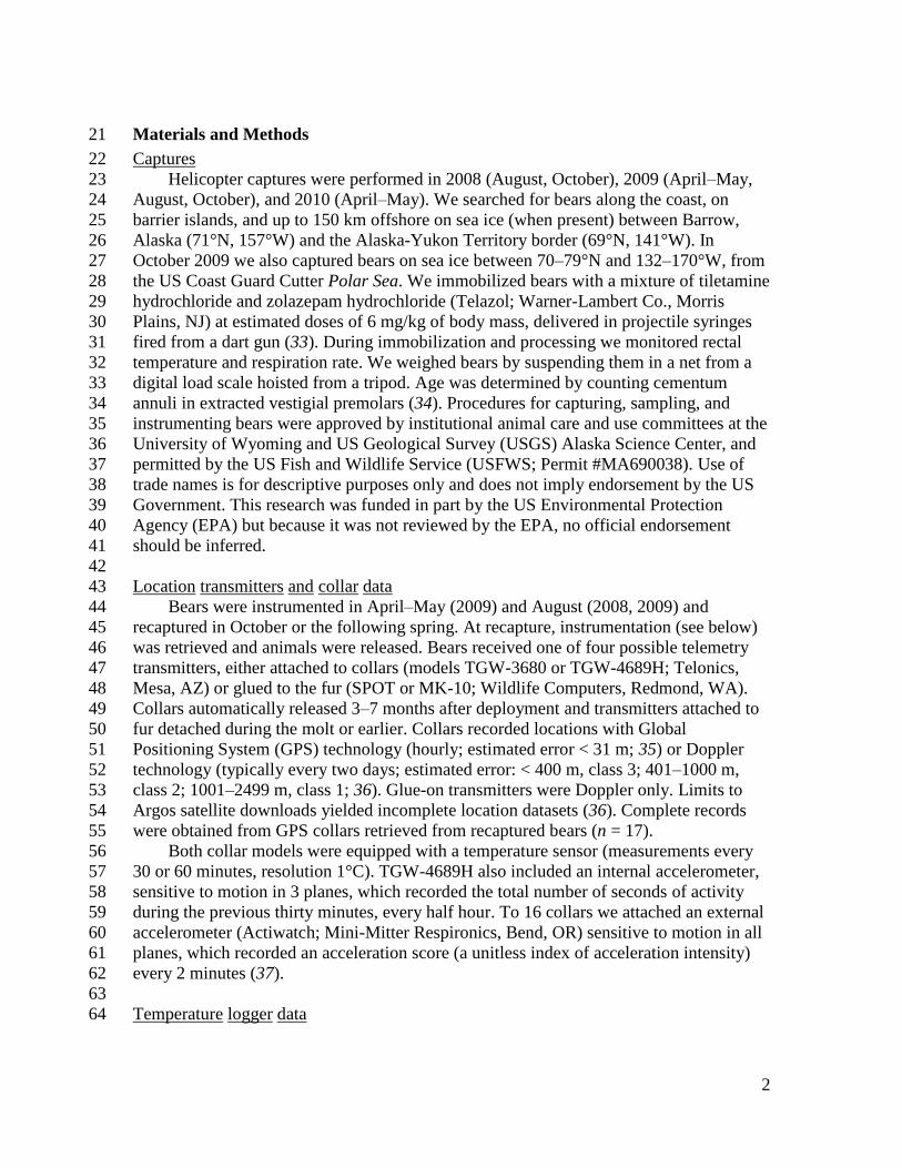
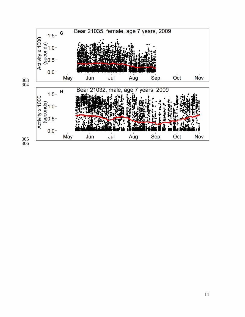
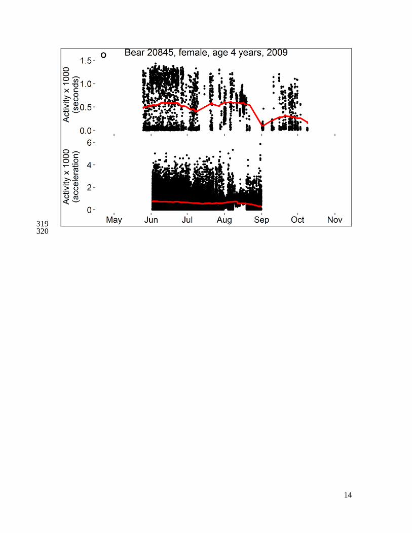
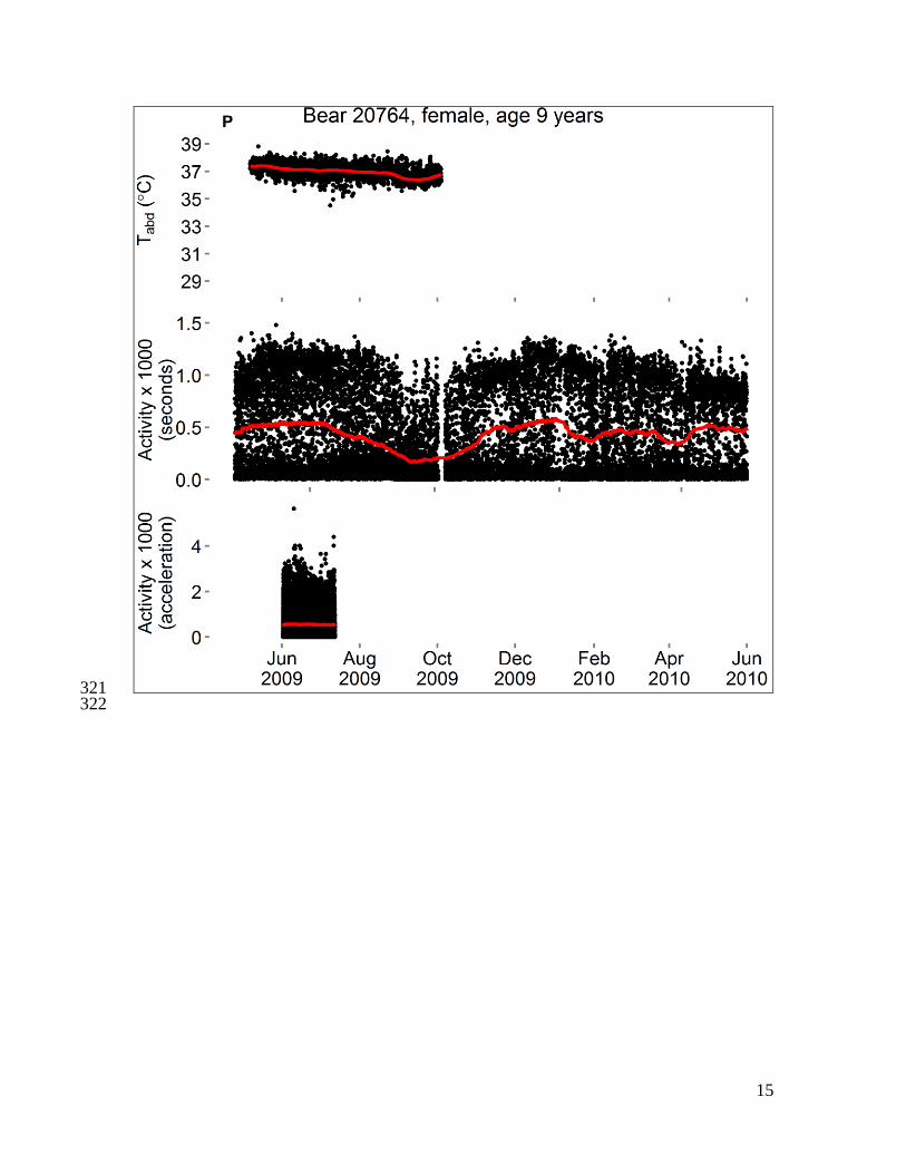
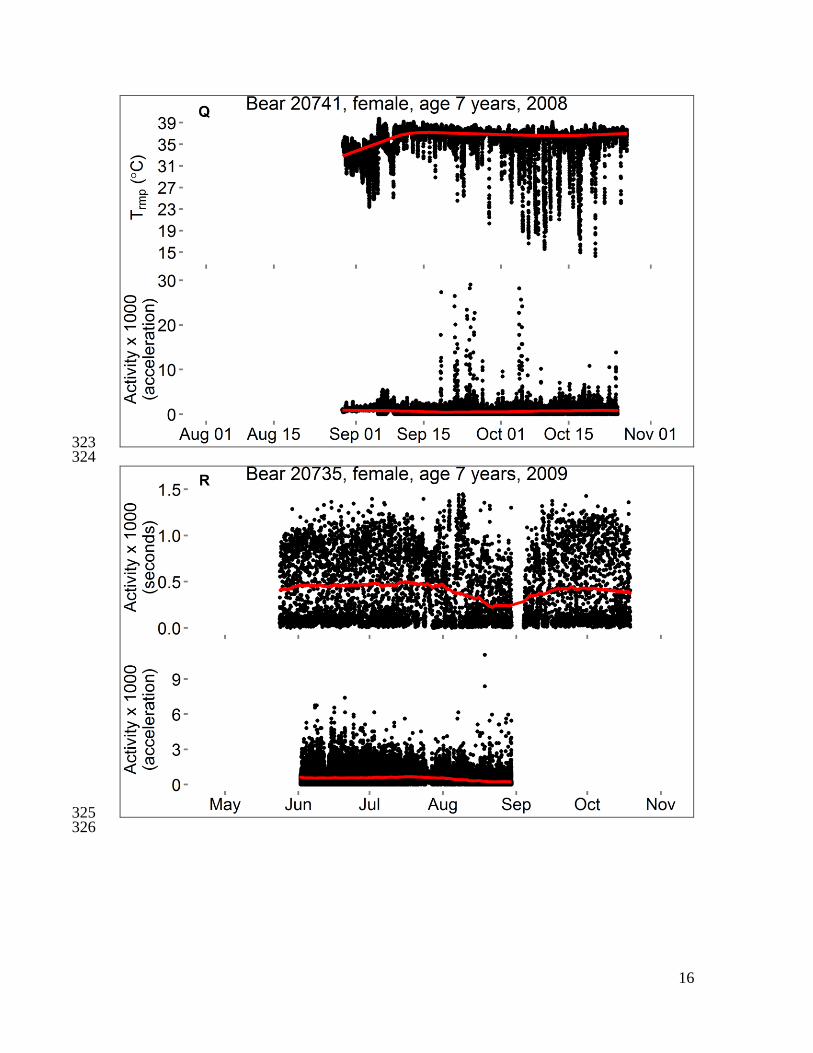
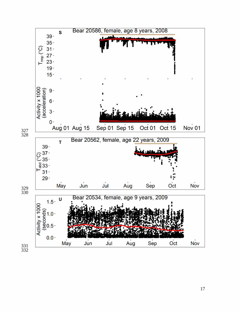
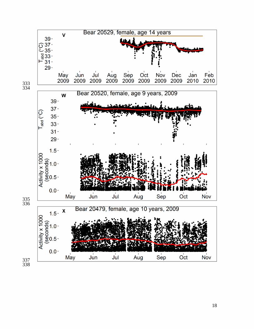
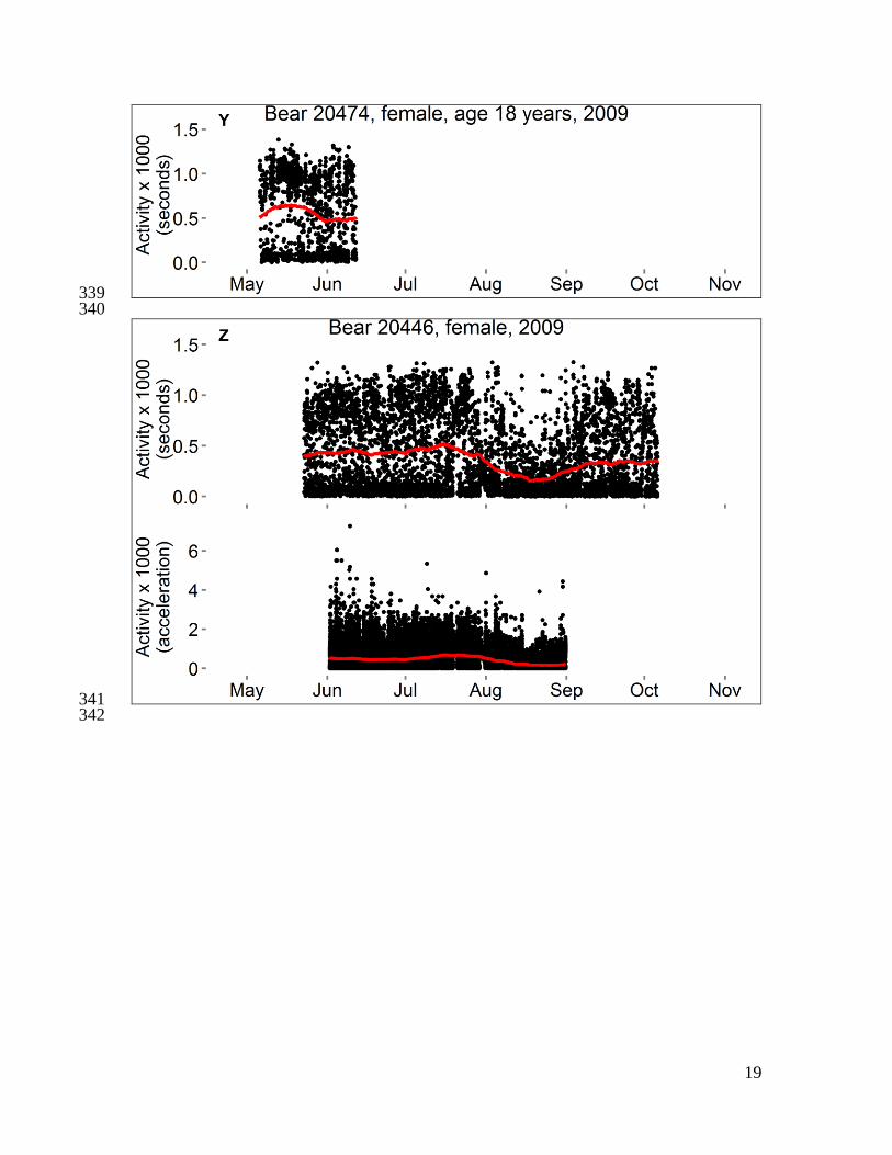
Fig. S1 351

Activity and body temperatures of polar bears in the Beaufort Sea, 2008–2010. Each 352

panel shows data from 1–3 variables for a single bear. Data censored ≤ 5 days after 353

capture and ≤ 1 hour before recapture. Temperature is either “Tabd” (hourly temperature 354

of a logger implanted into the abdomen) or “Trmp” (temperature of a logger implanted 355

beneath subcutaneous adipose tissue on the rump, recorded every 5–10 minutes), and red 356

line is the smoothed trend after seasonal decomposition analysis. Activity is either 357

“Activity (seconds)” (number of seconds of activity in previous half-hour) or “Activity 358

(acceleration)” (acceleration score recorded every two minutes), and red line is moving 359

average at center of 20-day window. For some bears, a horizontal bar spans the dates 360

during which bear location was unknown (gray) or was on shore except for short swims 361

(brown). The absence of a bar indicates the bear was offshore (swimming to or from sea 362

ice, or traveling on sea ice surface). Data from bear 20741 were presented in Durner et al. 363

(6). 364

365

22

366 367

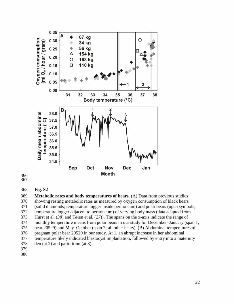
Fig. S2 368

Metabolic rates and body temperatures of bears. (A) Data from previous studies 369

showing resting metabolic rates as measured by oxygen consumption of black bears 370

(solid diamonds; temperature logger inside peritoneum) and polar bears (open symbols; 371

temperature logger adjacent to peritoneum) of varying body mass (data adapted from 372

Hurst et al. (38) and Tøien et al. (27)). The spans on the x-axis indicate the range of 373

monthly temperature means from polar bears in our study for December–January (span 1; 374

bear 20529) and May–October (span 2; all other bears). (B) Abdominal temperatures of 375

pregnant polar bear 20529 in our study. At 1, an abrupt increase in her abdominal 376

temperature likely indicated blastocyst implantation, followed by entry into a maternity 377

den (at 2) and parturition (at 3). 378

379

380

23

381 382

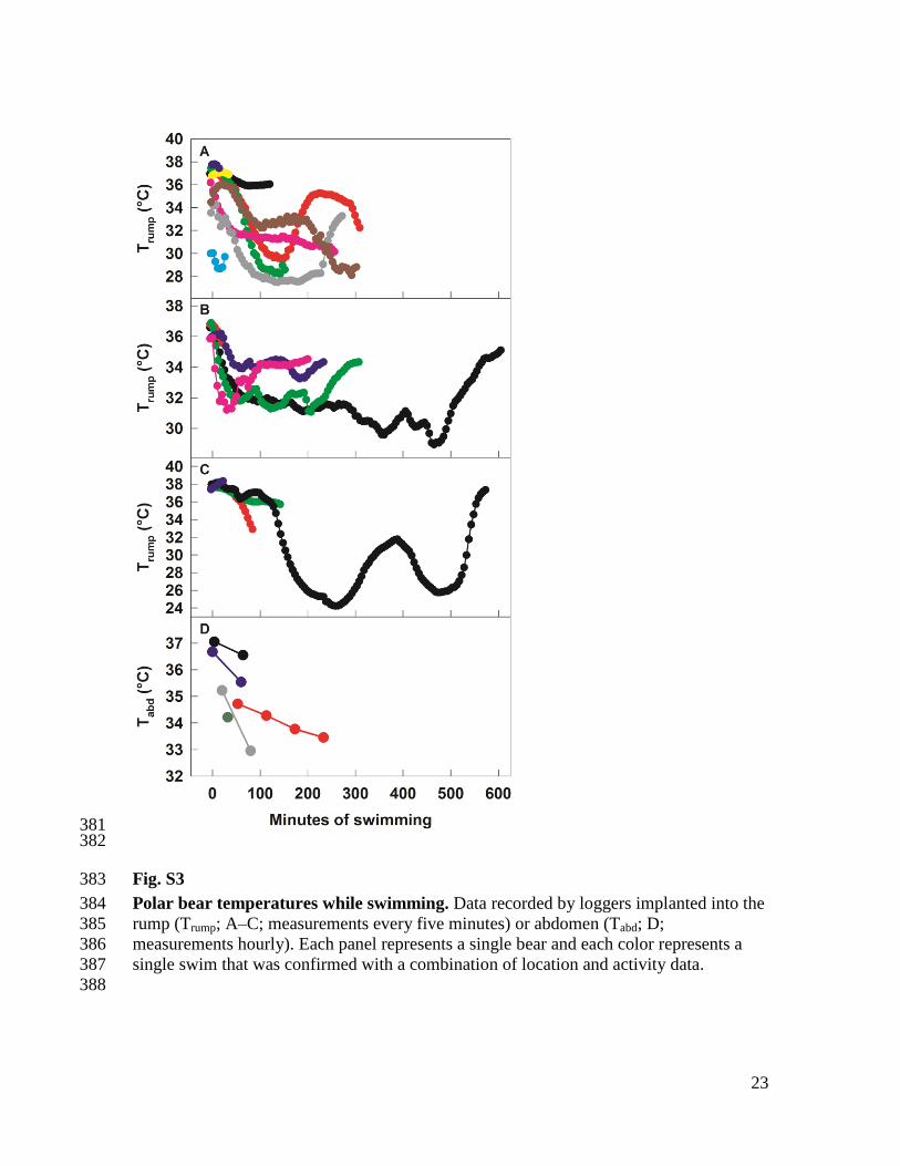
Fig. S3 383

Polar bear temperatures while swimming. Data recorded by loggers implanted into the 384

rump (Trump; A–C; measurements every five minutes) or abdomen (Tabd; D; 385

measurements hourly). Each panel represents a single bear and each color represents a 386

single swim that was confirmed with a combination of location and activity data. 387

388

24

389 390

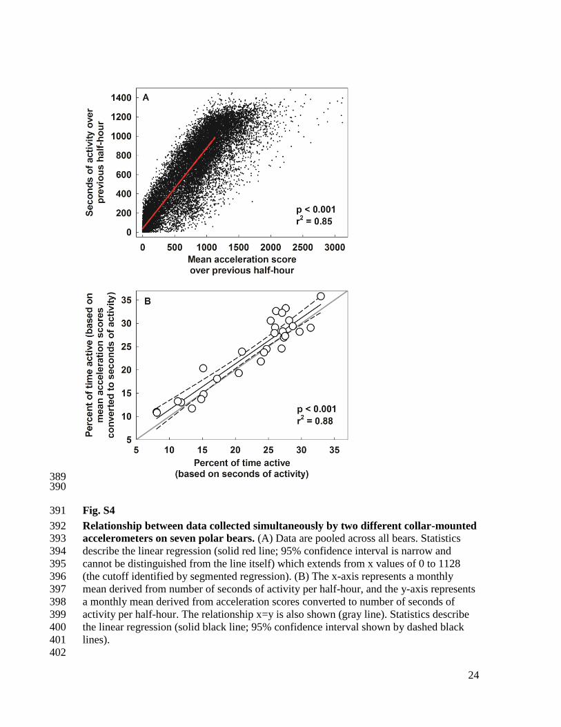
Fig. S4 391

Relationship between data collected simultaneously by two different collar-mounted 392 accelerometers on seven polar bears. (A) Data are pooled across all bears. Statistics 393

describe the linear regression (solid red line; 95% confidence interval is narrow and 394

cannot be distinguished from the line itself) which extends from x values of 0 to 1128 395

(the cutoff identified by segmented regression). (B) The x-axis represents a monthly 396

mean derived from number of seconds of activity per half-hour, and the y-axis represents 397

a monthly mean derived from acceleration scores converted to number of seconds of 398

activity per half-hour. The relationship x=y is also shown (gray line). Statistics describe 399

the linear regression (solid black line; 95% confidence interval shown by dashed black 400

lines). 401

402

25

403 404

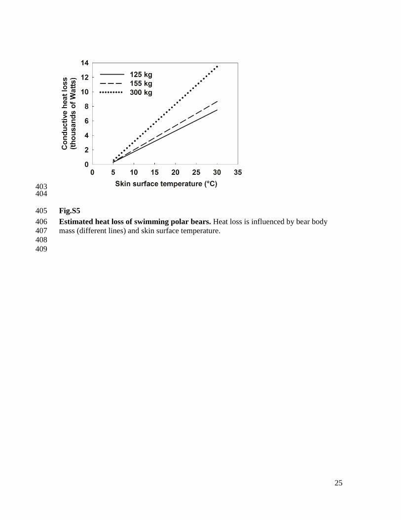
Fig.S5 405

Estimated heat loss of swimming polar bears. Heat loss is influenced by bear body 406

mass (different lines) and skin surface temperature. 407

408

409

26

Table S1. 410

Statistics of Welch t-tests comparing data collected from polar bears on shore and 411 on sea ice. Where present, data from 2008 and 2009 were combined. The variable of time 412

spent active is derived from both seconds of activity per half-hour, and from acceleration 413

scores converted to seconds of activity per half-hour. 414

415

Mean ± SE

Variable Month Shore Ice p t df

Time spent

active

July 11.8 24.6 ± 0.9 NA NA NA

August 21.4 ± 5.3 20.0 ± 1.9 0.80 0.26 7.50

September 17.8 ± 2.1 14.6 ± 1.1 0.21 1.33 13.54

October 19.2 ± 2.7 19.3 ± 1.8 0.99 -0.01 12.71

Movement

rate

July 0.12 0.31 ± 0.02 NA NA NA

August 0.16 ± 0.02 0.32 ± 0.01 <0.01 7.55 9.85

September 0.11 ± 0.02 0.33 ± 0.03 <0.01 -6.34 19.14

October 0.14 ± 0.04 0.40 ± 0.05 <0.01 -4.35 17.99

Abdominal

temperature

August 37.0 ± 0.2 36.8 ± 0.1 0.42 -0.88 4.50

September 36.8 ± 0.2 36.6 ± 0.1 0.48 -0.74 6.24

October 37.1 ± 0.2 36.8 ± 0.1 0.21 -1.44 5.13

416

417

27

Table S2. 418

Statistics of Welch t-tests comparing data collected in 2008 and 2009, from polar 419 bears on shore. Polar bears on sea ice were only sampled in 2009. The variable of time 420

spent active is derived from both seconds of activity per half-hour, and from acceleration 421

scores converted to seconds of activity per half-hour. 422

423

Mean ± SE

Variable Month 2008 2009 p t df

Time

spent

active

July NA 11.8 NA NA NA

August 28.4 ± 7.5 12.2 ± 2.7 0.12 2.03 3.73

September 18.6 ± 2.5 15.7 ± 4.5 0.60 0.58 3.33

October 18.7 ± 3.1 22.7 NA NA NA

Movement

rate

July NA 0.12 NA NA NA

August 0.16 ± 0.03 0.16 ± 0.02 NA NA NA

September 0.10 ± 0.02 0.16 ± 0.03 0.26 -1.50 2.17

October 0.14 ± 0.5 0.12 NA NA NA

424

28

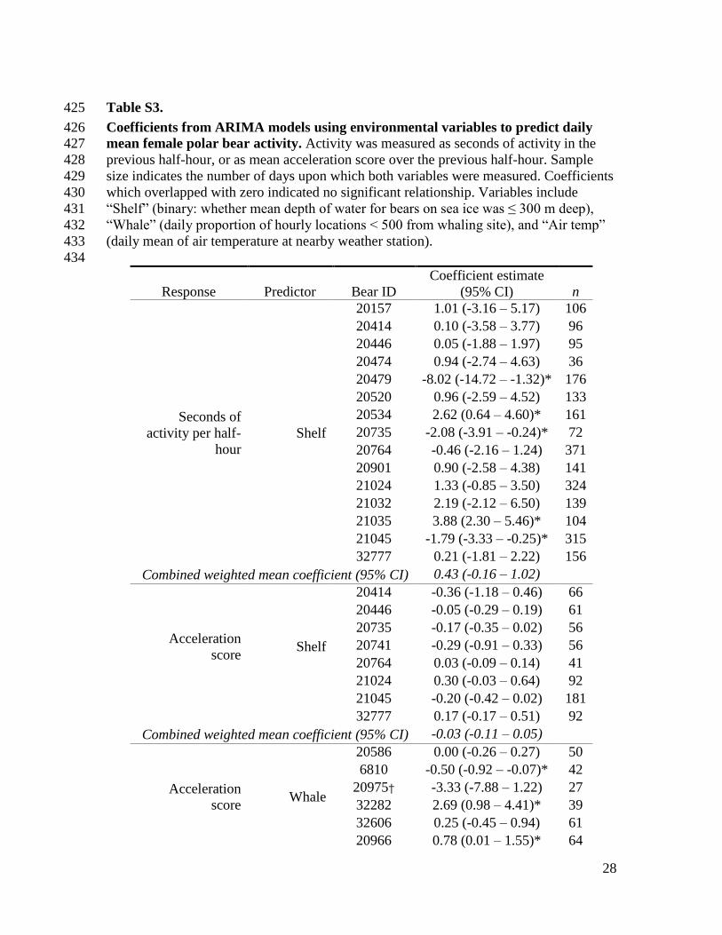
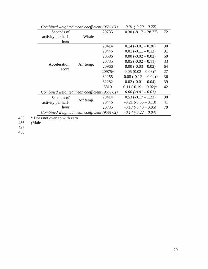
Table S3. 425

Coefficients from ARIMA models using environmental variables to predict daily 426 mean female polar bear activity. Activity was measured as seconds of activity in the 427

previous half-hour, or as mean acceleration score over the previous half-hour. Sample 428

size indicates the number of days upon which both variables were measured. Coefficients 429

which overlapped with zero indicated no significant relationship. Variables include 430

“Shelf” (binary: whether mean depth of water for bears on sea ice was ≤ 300 m deep), 431

“Whale” (daily proportion of hourly locations < 500 from whaling site), and “Air temp” 432

(daily mean of air temperature at nearby weather station). 433

434

Response Predictor Bear ID

Coefficient estimate

(95% CI) n

Seconds of

activity per half-

hour

Shelf

20157 1.01 (-3.16 – 5.17) 106

20414 0.10 (-3.58 – 3.77) 96

20446 0.05 (-1.88 – 1.97) 95

20474 0.94 (-2.74 – 4.63) 36

20479 -8.02 (-14.72 – -1.32)* 176

20520 0.96 (-2.59 – 4.52) 133

20534 2.62 (0.64 – 4.60)* 161

20735 -2.08 (-3.91 – -0.24)* 72

20764 -0.46 (-2.16 – 1.24) 371

20901 0.90 (-2.58 – 4.38) 141

21024 1.33 (-0.85 – 3.50) 324

21032 2.19 (-2.12 – 6.50) 139

21035 3.88 (2.30 – 5.46)* 104

21045 -1.79 (-3.33 – -0.25)* 315

32777 0.21 (-1.81 – 2.22) 156

Combined weighted mean coefficient (95% CI) 0.43 (-0.16 – 1.02)

Acceleration

score

Shelf

20414 -0.36 (-1.18 – 0.46) 66

20446 -0.05 (-0.29 – 0.19) 61

20735 -0.17 (-0.35 – 0.02) 56

20741 -0.29 (-0.91 – 0.33) 56

20764 0.03 (-0.09 – 0.14) 41

21024 0.30 (-0.03 – 0.64) 92

21045 -0.20 (-0.42 – 0.02) 181

32777 0.17 (-0.17 – 0.51) 92

Combined weighted mean coefficient (95% CI) -0.03 (-0.11 – 0.05)

Acceleration

score Whale

20586 0.00 (-0.26 – 0.27) 50

6810 -0.50 (-0.92 – -0.07)* 42

20975† -3.33 (-7.88 – 1.22) 27

32282 2.69 (0.98 – 4.41)* 39

32606 0.25 (-0.45 – 0.94) 61

20966 0.78 (0.01 – 1.55)* 64

29

Combined weighted mean coefficient (95% CI) -0.01 (-0.20 – 0.22)

Seconds of

activity per half-

hour

Whale

20735 10.30 (-8.17 – 28.77) 72

Acceleration

score

Air temp.

20414 0.14 (-0.01 – 0.30) 30

20446 0.01 (-0.11 – 0.12) 31

20586 0.00 (-0.02 – 0.02) 50

20735 0.05 (-0.02 – 0.11) 33

20966 0.00 (-0.03 – 0.02) 64

20975† 0.05 (0.02 – 0.08)* 27

32255 -0.08 (-0.12 – -0.04)* 36

32282 0.02 (-0.01 – 0.04) 39

6810 0.11 (-0.19 – -0.02)* 42

Combined weighted mean coefficient (95% CI) 0.00 (-0.01 – 0.01)

Seconds of

activity per half-

hour

Air temp.

20414 0.53 (-0.17 – 1.23) 30

20446 -0.21 (-0.55 – 0.13) 41

20735 -0.17 (-0.40 – 0.05) 70

Combined weighted mean coefficient (95% CI) -0.14 (-0.22 – 0.04)

* Does not overlap with zero 435

†Male 436

437

438

30

Table S4. 439

Hourly locations recorded from GPS telemetry transmitters on female polar bears 440 on shore between August 1

st and November 1

st. Data from 2008 and 2009 were pooled. 441

Expected total number of locations is the number of hours between capture and recapture 442

of bears. Actual number of locations is fewer than expected because weather and 443

equipment failure occasionally prevented transmitter function. For each bear, a total of 444

the number of locations that were within 2000 m and 500 m of three sites where bowhead 445

whale carcasses are deposited after human harvest is also presented. 446

447

Number of hourly locations

BearID Year

Expected

total

Actual total

(% of expected)

Within 2000 m

(% of actual)

Within 500 m

(% of actual)

32282 2008 1103 1099 (99) 431 (39) 41 (4)

20735 2009 1677 1666 (99) 885 (53) 59 (4)

32255 2008 1030 1017 (99) 0 (0) 0 (0)

20966 2008 1700 1675 (98) 898 (54) 107 (6)

20586 2008 1386 1363 (98) 1084 (80) 931 (68)

20446 2009 945 926 (98) 14 (2) 1 (0.1)

6810 2008 1193 1144 (96) 701 (61) 649 (57)

32608 2008 1193 1041 (87) 537 (52) 50 (5)

20982 2008 1517 1104 (73) 242 (22) 28 (3)

32606 2008 402 279 (69) 155 (56) 23 (8)

20965 2008 1611 1031 (64) 159 (15) 20 (2)

20974 2008 1732 899 (52) 0 (0) 0 (0)

20414 2009 1909 930 (49) 0 (0) 0 (0)

20492 2008 1823 818 (45) 386 (47) 78 (10)

20975* 2008 1659 685 (41) 307 (45) 25 (4)

*Male 448

449

31

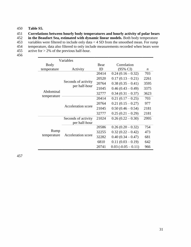
Table S5. 450

Correlations between hourly body temperatures and hourly activity of polar bears 451 in the Beaufort Sea, estimated with dynamic linear models. Both body temperature 452

variables were filtered to include only data < 4 SD from the smoothed mean. For rump 453

temperature, data also filtered to only include measurements recorded when bears were 454

active for > 2% of the previous half-hour. 455

456

Variables

Body

temperature Activity

Bear

ID

Correlation

(95% CI) n

Abdominal

temperature

Seconds of activity

per half-hour

20414 0.24 (0.16 – 0.32) 703

20520 0.17 (0.13 – 0.21) 2261

20764 0.38 (0.35 – 0.41) 3595

21045 0.46 (0.43 – 0.49) 3375

32777 0.34 (0.31 – 0.37) 3623

Acceleration score

20414 0.21 (0.17 – 0.25) 703

20764 0.21 (0.15 – 0.27) 977

21045 0.50 (0.46 – 0.54) 2181

32777 0.25 (0.21 – 0.29) 2181

Rump

temperature

Seconds of activity

per half-hour

21024 0.26 (0.22 – 0.30) 2995

Acceleration score

20586 0.26 (0.20 – 0.32) 754

32255 0.32 (0.22 – 0.42) 473

32282 0.40 (0.34 – 0.47) 681

6810 0.11 (0.03 – 0.19) 642

20741 0.03 (-0.05 – 0.11) 966

457

32

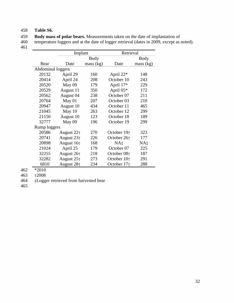
Table S6. 458

Body mass of polar bears. Measurements taken on the date of implantation of 459

temperature loggers and at the date of logger retrieval (dates in 2009, except as noted). 460

461

Implant Retrieval

Bear Date

Body

mass (kg) Date

Body

mass (kg)

Abdominal loggers

20132 April 29 160 April 22* 148

20414 April 24 208 October 10 243

20520 May 09 179 April 17* 229

20529 August 11 350 April 05* 172

20562 August 04 238 October 07 211

20764 May 01 207 October 03 210

20947 August 10 434 October 11 465

21045 May 19 263 October 12 299

21150 August 10 123 October 18 189

32777 May 09 196 October 19 299

Rump loggers

20586 August 22† 270 October 19† 323

20741 August 23† 226 October 26† 177

20898 August 16† 168 NA‡ NA‡

21024 April 25 179 October 07 225

32255 August 26† 218 October 08† 187

32282 August 25† 273 October 10† 291

6810 August 28† 234 October 17† 288

*2010 462

†2008 463

‡Logger retrieved from harvested bear 464

465

33

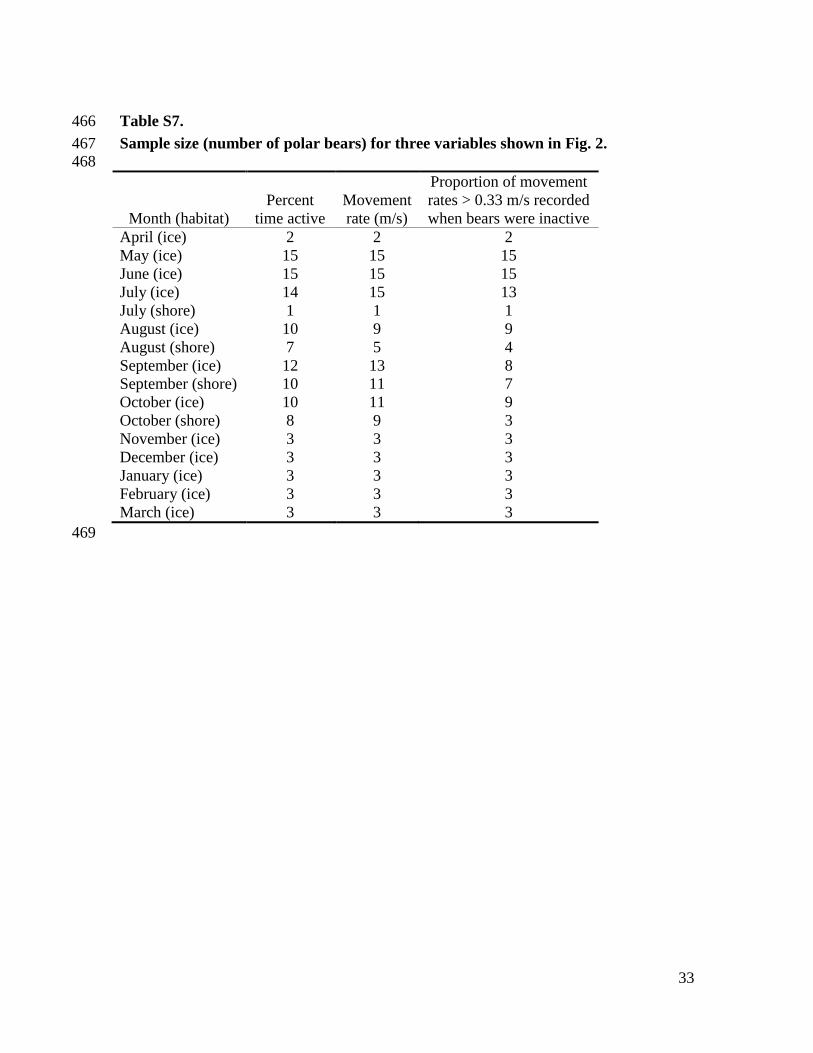
Table S7. 466

Sample size (number of polar bears) for three variables shown in Fig. 2. 467 468

Month (habitat)

Percent

time active

Movement

rate (m/s)

Proportion of movement

rates > 0.33 m/s recorded

when bears were inactive

April (ice) 2 2 2

May (ice) 15 15 15

June (ice) 15 15 15

July (ice) 14 15 13

July (shore) 1 1 1

August (ice) 10 9 9

August (shore) 7 5 4

September (ice) 12 13 8

September (shore) 10 11 7

October (ice) 10 11 9

October (shore) 8 9 3

November (ice) 3 3 3

December (ice) 3 3 3

January (ice) 3 3 3

February (ice) 3 3 3

March (ice) 3 3 3

469