Embed Size (px)
Citation preview
Supplementary Materials to
Changing Spatial Epidemiology of Pertussis inContinental USA
Marc ChoisyMIVEGEC (UM1-UM2-CNRS 5290-IRD 224),Centre IRD, 911 avenue Agropolis BP 64501,
34394 Montpellier Cedex 5, [email protected]
Pejman RohaniDepartment of Ecology and Evolutionary Biology and
Center for the Study of Complex Systems,University of Michigan, Ann Arbor, MI, USA
Fogarty International Center,National Institutes of Health, Bethesda, MD 20892, USA
1
1 Selection of the two analyzed eras
Given a long (1970–1990) and almost uninformative period of time chara-caterizing the US pertussis notification case time series, we performed ouranalyses on two separate eras, before and after this central part. The mainconcerns about selecting a portion of the data to perform our analysis are,first, the arbitrary choice and, second, the robustness of the results respec-tive to this choice. We addressed these concerns by examining the behaviorsof the distribution of the pairwise correlation coefficients (fig. S1A and B),the number of states above and below the CCS (fig. S1C and D), the spatialcorrelation functions (not shown because involving too many figures) andthe global wavelet spectra (not shown because involving too many figures)calculated on the 1951-x (in red) and x-2010 (in blue) time periods when xvaries between 1951 and 2010. All these analyses identified sharp transitionsaround 1963 and 2002, and we based the selection of the two analyzed erason these transitions. Moreover, the results presented in the article for thefirst era with x =1962 were fairly robust with respect to x. Finally, select-ing the time period before or after the wavelet decomposition did not affectsignificantly the results.
2 Decomposition of the signal
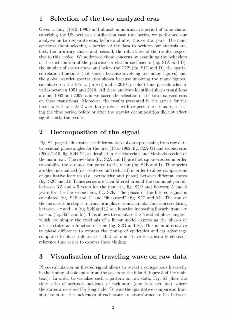
Fig. S2, page 4, illustrates the different steps of data processing from raw datato residual phase angles for the first (1951-1962, fig. S2A-G) and second eras(2002-2010, fig. S2H-N), as detailed in the Materials and Methods section ofthe main text. The raw data (fig. S2A and H) are first square-rooted in orderto stabilize the variance compared to the mean (fig. S2B and I). Time seriesare then normalized (i.e. centered and reduced) in order to allow comparisonsof qualitative features (i.e. periodicity and phase) between different states(fig. S2C and J). Times series are then filtered around the dominant period:between 3.5 and 4.5 years for the first era, fig. S2D and between 5 and 6years for the the second era, fig. S2K. The phase of the filtered signal iscalculated (fig. S2E and L) and “linearized” (fig. S2F and M). The aim ofthe linearization step is to transform phase from a circular function oscillatingbetween−π and +π (fig. S2E and L) to a function increasing linearly from−πto +∞ (fig. S2F and M). This allows to calculate the “residual phase angles”which are simply the residuals of a linear model expressing the phases ofall the states as a function of time (fig. S2G and N). This is an alternativeto phase difference to express the timing of epidemics and its advantagecompared to phase difference is that we don’t have to arbitrarily choose areference time series to express these timings.
3 Visualisation of traveling wave on raw data
Phase calculation on filtered signal allows to reveal a conspicuous hierarchyin the timing of epidemics from the coasts to the inland (figure 3 of the maintext). In order to visualise such a pattern on raw data, Fig. S3 plots thetime series of pertussis incidence of each state (one state per line), wherethe states are ordered by longitude. To ease the qualitative comparison fromstate to state, the incidences of each state are transformed to lies between
2

correlation coefficient
num
ber
0.0 0.2 0.4 0.6 0.8
05
1525
35
1951−19801981−2010A
1960 1980 20000.
00.
20.
40.
6separating year
corr
elat
ion
coef
ficie
nt
beforeafter
B
population size x1000
with
no
notif
icat
ion
prop
ortio
n of
mon
ths
0 10000 20000 30000
0.0
0.2
0.4
0.6
0.8
●●●
●
●●
●
●
●
●●
●●
●
●
●
●●
●●
●
●
●
●
●
●
●
● ●
●
●●
●
●
●
●●
● ●
●
● ●
●●
●●
●●
●
●
●
●
●●
●
●
●
●
●●
●
●
●●
●●
●
●●
●
●
●
●
●●
●
●●
●
●
●
●
●
●
●
●
●
●
●
●
●
●
●
●
●
●
●
●
1951−1980 1981−2010
C●●●●●●●●
●
●●●●
●●●●●●●●●●●●●●●●●●●●●●●●●●●●●●●●●●●●●●●●●●●●
1960 1980 2000
010
2030
40
separating year
num
ber
of s
tate
s ab
ove
CC
S
●●●●●●●●●●●●●●●●●●●●●●●●●●●●●●●●●●●●●●●●●
●●●●●●
●●●
●
●
●●●●●
beforeafter
D
Figure S 1: Variation of the pairwise correlation distribution and CCS overthe 1951-x and x-2010 time periods when x varies between 1951 and 2010.(A) Distributions of the pairwise correlation coefficient for the particularcase of x =1980. (B) Changes in the distributions when x varies between1951 and 2010. The lines are the mean values of the distribution and thecolored areas are the 50% confidence intervals. The vertical lines show thefirst days of 1963 and 2002. (C) CCS for the particular case of x =1980. (D)Changes in the number of states above the CCS when x varies between 1951and 2010. The vertical lines show the first days of 1963 and 2002.
3
050
015
00in
cide
nce
A
010
2030
40in
cide
nce
B
−2
02
46
norm
. in
cid.
C
−1.
5−
0.5
0.5
1.5
filte
red
com
pone
ntD
−3
−1
12
3ph
ase
angl
e
E
05
1020
phas
e an
gle
F
−3
−1
12
3re
sidu
al p
hase
ang
le
1952 1954 1956 1958 1960 1962year
G
040
080
0in
cide
nce
H
010
2030
inci
denc
e
I
−2
02
46
norm
. in
cid.
J
−0.
50.
51.
0fil
tere
d co
mpo
nent K
−3
−1
12
3ph
ase
angl
e
L
05
1020
phas
e an
gle
M
−3
−1
12
3re
sidu
al p
hase
ang
le
2002 2004 2006 2008 2010year
N
Figure S 2: Decomposition of the signal. See text for explanations.
4

0 and 1 (and called “relative number of cases”). One can thus guess in thefirst era of fig. S3 the traveling wave that is much more clearly visible andquantified on figure 3 of the main text. There is no such clear structure inthe second era.
1952 1956 1960
1020
3040
year
stat
es o
rder
ed b
y lo
ngitu
deE
W2003 2007 2011
1020
3040
stat
es o
rder
ed b
y lo
ngitu
de
E
W 0.0
0.2
0.4
0.6
0.8
1.0
rela
tive
num
ber
of c
ases
Figure S 3: Relative numbers of notification cases for each of the 49 statesordered according to the longitude of their population centers from west(bottom) to east (top) over the periods 1951–1962 (left panel) and 2002–2010 (right panel). States are: OR (line 1), WA (2), CA (3), NV (4), ID (5),UT (6), AZ (7), MT (8), WY (9), NM (10), CO (11), ND (12), SD (13), NE(14), TX (15), OK (16), KS (17), MN (18), IA (19), AR (20), MO (21), LA(22), MS (23), WI (24), IL (25), AL (26), TN (27), IN (28), KY (29), MI(30), GA (31), OH (32), FL (33), SC (34), WV (35), NC (36), VA (37), PA(38), DC (39), MD (40), DE (41), NY (42), NJ (43), CT (44), VT (45), NH(46), RI (47), MA (48), ME (49).
4 Phase-population size relationship
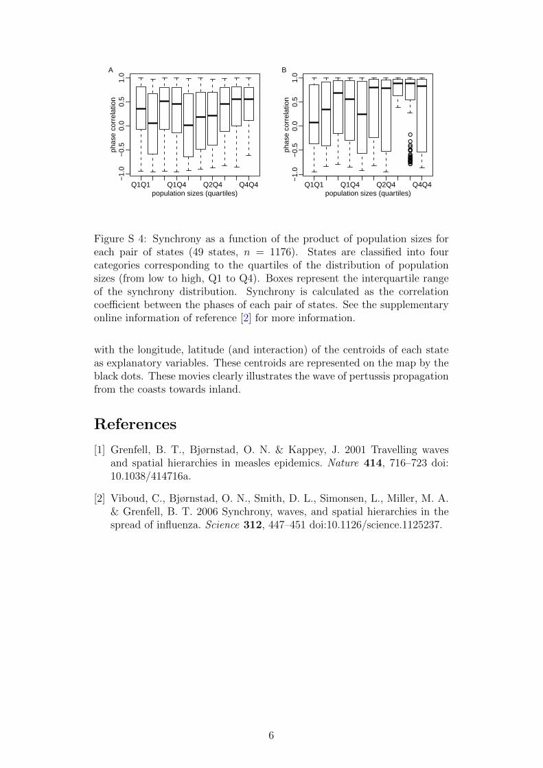
In order to test the gravity mechanism on our data, we drew the relationshipbetween residual phase angles and their corresponding population size (Fig. 4in the main text), similarly to what was done in reference [1] (figure 4C in thisreference). Since, in the gravity model, the timing of epidemics is expected todepend on the product of the population sizes, we also plotted the correlationbetween phases as a function of the product of population sizes for each pairof states (fig. S4), as done in reference [2] (figures 4C and D in this reference).
5 Movies of the pertussis spatial dynamics
Two movies of the spatial dynamics of pertussis in the US can be seen athttp://marcchoisy.free.fr/pertussis. In each movie, the upper panelshows the time series of the pertussis incidence (number of reported newcases divided by population size) aggregated for the all USA. The verticalblue bar refers to the time point to which the map in the lower panel corre-sponds. The map of the first movie shows the values of the filtered (betweenperiods of 3.5 and 4.5 years) time series for each state whereas the map ofthe second movie depicts spatially smoothed values, using a loess regression
5
Q1Q1 Q1Q4 Q2Q4 Q4Q4
−1.
0−
0.5
0.0
0.5
1.0
population sizes (quartiles)
phas
e co
rrel
atio
n
A
●
●●●●●●●
●●
●●●●●●●●●●
●
●
●●
Q1Q1 Q1Q4 Q2Q4 Q4Q4
−1.
0−
0.5
0.0
0.5
1.0
population sizes (quartiles)
phas
e co
rrel
atio
n
B
Figure S 4: Synchrony as a function of the product of population sizes foreach pair of states (49 states, n = 1176). States are classified into fourcategories corresponding to the quartiles of the distribution of populationsizes (from low to high, Q1 to Q4). Boxes represent the interquartile rangeof the synchrony distribution. Synchrony is calculated as the correlationcoefficient between the phases of each pair of states. See the supplementaryonline information of reference [2] for more information.
with the longitude, latitude (and interaction) of the centroids of each stateas explanatory variables. These centroids are represented on the map by theblack dots. These movies clearly illustrates the wave of pertussis propagationfrom the coasts towards inland.
References
[1] Grenfell, B. T., Bjørnstad, O. N. & Kappey, J. 2001 Travelling wavesand spatial hierarchies in measles epidemics. Nature 414, 716–723 doi:10.1038/414716a.
[2] Viboud, C., Bjørnstad, O. N., Smith, D. L., Simonsen, L., Miller, M. A.& Grenfell, B. T. 2006 Synchrony, waves, and spatial hierarchies in thespread of influenza. Science 312, 447–451 doi:10.1126/science.1125237.
6