J. Broida UCSD Fall 2009

Phys 130B QM II

Supplementary Notes on Mathematics

Part I: Linear Algebra

1 Linear Transformations

Let me very briefly review some basic properties of linear transformations and theirmatrix representations that will be useful to us in this course. Most of this shouldbe familiar to you, but I want to make sure you know my notation and understandhow I think about linear transformations. I assume that you are already familiarwith the three elementary row operations utilized in the Gaussian reduction ofmatrices:

(α) Interchange two rows.(β) Multiply one row by a nonzero scalar.(γ) Add a scalar multiple of one row to another.

I also assume that you know how to find the inverse of a matrix, and you knowwhat a vector space is.

If V is an n-dimensional vector space over a field F (which you can think of aseither R or C), then a linear transformation on V is a mapping T : V → V withthe property that for all x, y ∈ V and a ∈ F we have

T (x + y) = T (x) + T (y) and T (ax) = aT (x) .

We will frequently write Tx rather than T (x). That T (0) = 0 follows either byletting a = 0 or noting that T (x) = T (x + 0) = T (x) + T (0).

By way of notation, we will write T ∈ L(V ) if T is a linear transformation fromV to V . A more general notation very often used is to write T ∈ L(U, V ) to denotea linear transformation T : U → V from a space U to a space V .

A set of vectors {v1, . . . , vn} is said to be linearly independent if∑n

i=1 aivi =0 implies that ai = 0 for all i = 1, . . . , n. The set {vi} is also said to span V ifevery vector in V can be written as a linear combination of the vi. A basis for Vis a set of linearly independent vectors that also spans V . The dimension of V isthe (unique) number of vectors in any basis.

A simple but extremely useful fact is that every vector x ∈ V has a uniqueexpansion in terms of any given basis {ei}. Indeed, if we have two such expansionsx =

∑ni=1 xiei and x =

∑ni=1 x′

iei, then∑n

i=1(xi − x′i)ei = 0. But the ei are

linearly independent by definition so that xi −x′i = 0 for each i, and hence we must

have xi = x′i and the expansion is unique as claimed. The scalars xi are called the

components of x.

1

Now suppose we are given a set {v1, v2, . . . , vr} of linearly independent vec-tors in a finite-dimensional space V with dimV = n. Since V always has a basis{e1, e2, . . . , en}, the set of n + r vectors {v1, . . . , vr, e1, . . . , en} will necessarily spanV . We know that v1, . . . , vr are linearly independent, so check to see if e1 can bewritten as a linear combination of the vi’s. If it can, then delete it from the set. Ifit can’t, then add it to the vi’s. Now go to e2 and check to see if it can be writtenas a linear combination of {v1, . . . , vr, e1}. If it can, delete it, and if it can’t, thenadd it to the set. Continuing in this manner, we will eventually arrive at a subsetof {v1, . . . , vr, e1, . . . , en} that is linearly independent and spans V . In other words,we have extended the set {v1, . . . , vr} to a complete basis for V . The fact that thiscan be done (at least in principle) is an extremely useful tool in many proofs.

A very important characterization of linear transformations that we may finduseful is the following. Define the set

KerT = {x ∈ V : Tx = 0} .

The set KerT ⊂ V is called the kernel of T . In fact, it is not hard to showthat KerT is actually a subspace of V . Recall that a mapping T is said to beone-to-one if x 6= y implies Tx 6= Ty. The equivalent contrapositive statementof this is that T is one-to-one if Tx = Ty implies x = y. Let T be a lineartransformation with KerT = {0}, and suppose Tx = Ty. Then by linearity wehave Tx − Ty = T (x − y) = 0. But KerT = {0} so we conclude that x − y = 0or x = y. In other words, the fact that KerT = {0} means that T must be one-to-one. Conversely, if T is one-to-one, then the fact that we always have T (0) = 0means that KerT = {0}. Thus a linear transformation is one-to-one if and onlyif KerT = {0}. A linear transformation T with KerT = {0} is said to be anonsingular transformation.

If V has a basis {ei}, then any x ∈ V has a unique expansion which we will writeas x = xiei. Note that here I am using the Einstein summation convention

where repeated indices are summed over. (The range of summation is always clearfrom the context.) Thus xiei is a shorthand notation for

∑ni=1 xiei. Since we will

almost exclusively work with Cartesian coordinates, there is no difference betweensuperscripts and subscripts, and I will freely raise or lower indices as needed fornotational clarity. In general, the summation convention should properly be appliedto an upper and a lower index, but we will sometimes ignore this, particularly whenit comes to angular momentum operators. Note also that summation indices aredummy indices. By this we mean that the particular letter used to sum over isirrelevant. In other words, xiei is the same as xkek, and we will frequently relabelindices in many of our calculations.

In any case, since T is a linear map, we see that T (x) = T (xiei) = xiT (ei) andhence a linear transformation is fully determined by its values on a basis. Since Tmaps V into V , it follows that Tei is just another vector in V , and hence we canwrite

Tei = ejaji (1)

where the scalar coefficients aji define the matrix representation of T with re-

spect to the basis {ei}. We sometimes write [T ] = (aij) to denote the fact that the

2

n×n matrix A = (aij) is the matrix representation of T . (And if we need to be clear

just what basis the matrix representation is with respect to, we will write [T ]e.) Besure to note that it is the row index that is summed over in this equation. This isnecessary so that the composition ST of two linear transformations S and T has amatrix representation [ST ] = AB that is the product of the matrix representations[S] = A of S and [T ] = B of T taken in the same order.

We will denote the set of all n × n matrices over the field F by Mn(F), andthe set of all m× n matrices over F by Mm×n(F). Furthermore, if A ∈ Mm×n(F),we will label the rows of A by subscripts such as Ai, and the columns of A bysuperscripts such as Aj . It is important to realize that each row vector Ai is justa vector in Fn, and each column vector Aj is just a vector in Fm. Therefore therows of A form a subspace of Rn called the row space and denoted by row(A).Similarly, the columns form a subspace of Fm called the column space col(A).The dimension of row(A) is called the row rank rr(A) of A, and dim col(A) iscalled the column rank cr(A).

What happens if we perform elementary row operations on A? Since all we dois take linear combinations of the rows, it should be clear that the row space won’tchange, and hence rr(A) is also unchanged. However, the components of the columnvectors get mixed up, so it isn’t at all clear just what happens to either col(A) orcr(A). In fact, while col(A) will change, it turns out that cr(A) remains unchanged.

Probably the easiest way to see this is to consider those columns of A that arelinearly dependent ; and with no loss of generality we can call them A1, . . . , Ar.Then their linear dependence means there are nonzero scalars x1, . . . , xr such that∑r

i=1 Aixi = 0. In full form this is

a11

...am1

x1 + · · · +

a1r

...amr

xr = 0.

But this is a system of m linear equations in r unknowns, and we have seen that thesolution set doesn’t change under row equivalence. In other words,

∑ri=1 Aixi = 0

for the same coefficients xi. Then the same r columns of A are linearly dependent,and hence both A and A have the same (n − r) independent columns, i.e., cr(A) =cr(A). (There can’t be more dependent columns of A than A because we can applythe row operations in reverse to go from A to A. If A had more dependent columns,then when we got back to A we would have more than we started with.)

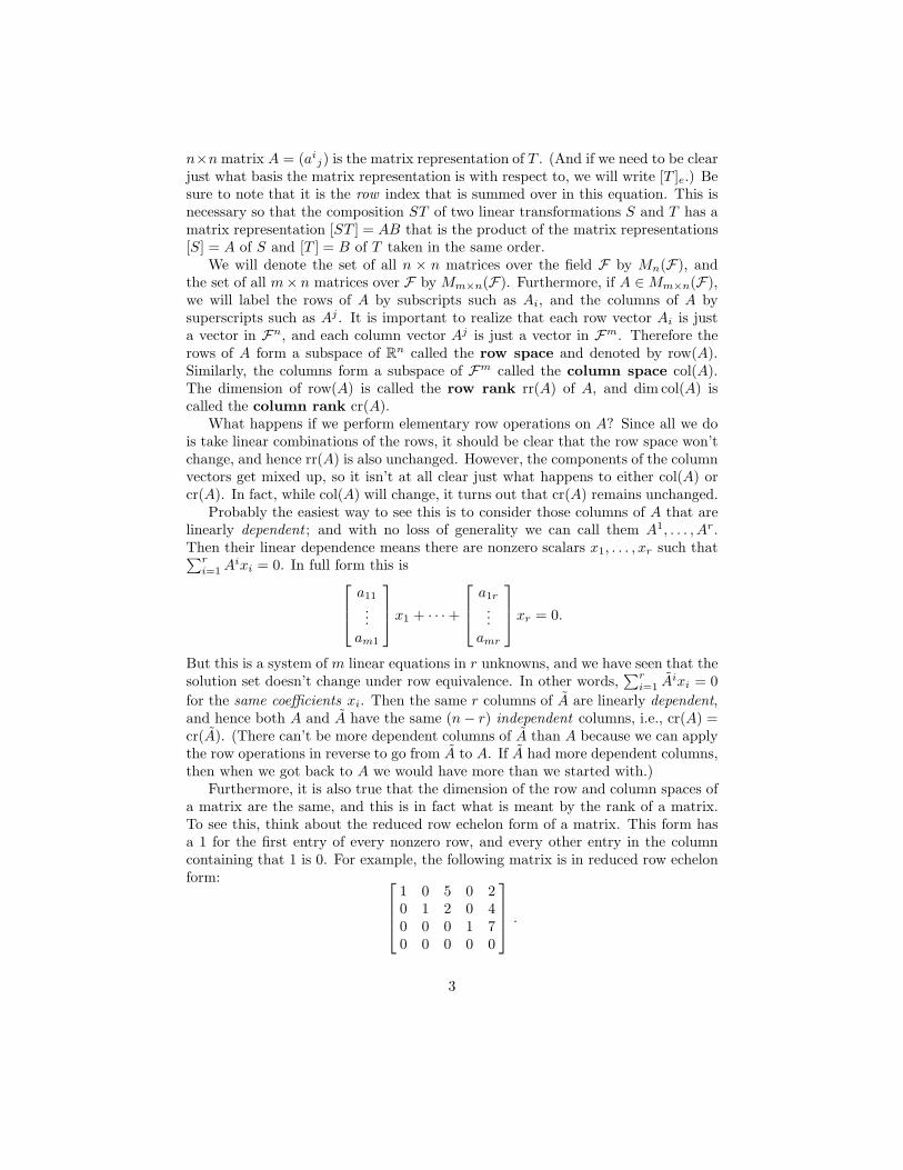
Furthermore, it is also true that the dimension of the row and column spaces ofa matrix are the same, and this is in fact what is meant by the rank of a matrix.To see this, think about the reduced row echelon form of a matrix. This form hasa 1 for the first entry of every nonzero row, and every other entry in the columncontaining that 1 is 0. For example, the following matrix is in reduced row echelonform:

1 0 5 0 20 1 2 0 40 0 0 1 70 0 0 0 0

.

3

Note that every column either consists entirely of a single 1, or is a linear combina-tion of columns that each have only a single 1. In addition, the number of columnscontaining that single 1 is the same as the number of nonzero rows. Therefore therow rank and column rank are the same, and this common number is called therank of a matrix.

If A ∈ Mn(F) is an n × n matrix that is row equivalent to the identity matrixI, then A has rank n, and we say that A is nonsingular. If rankA < n then A issaid to be singular. It can be shown that a matrix is invertible (i.e., A−1 exists) ifand only if it is nonsingular.

Now let A ∈ Mm×n(F) and B ∈ Mn×r(F) be such that the product AB isdefined. Since the (i, j)th entry of AB is given by (AB)ij =

∑k aikbkj , we see that

the ith row of AB is given by a linear combination of the rows of B:

(AB)i =

(∑

k

aikbk1, . . . ,∑

k

aikbkr

)=∑

k

aik (bk1, . . . , bkr) =∑

k

aikBk. (2a)

This shows that the row space of AB is a subspace of the row space of B. Anotherway to write this is to observe that

(AB)i =

(∑

k

aikbk1, . . . ,∑

k

aikbkr

)

= (ai1, . . . , ain)

b11 · · · b1r

......

bn1 · · · bnr

= AiB. (2b)

Similarly, for the columns of a product we find that the jth column of AB is alinear combination of the columns of A:

(AB)j =

∑k a1kbkj

...∑k amkbkj

=

n∑

k=1

a1k

...amk

bkj =

n∑

k=1

Akbkj (3a)

and therefore the column space of AB is a subspace of the column space of A. Wealso have the result

(AB)j =

∑k a1kbkj

...∑k amkbkj

=

a11 · · · a1n

......

am1 · · · amn

b1j

...bnj

= ABj . (3b)

These formulas will be quite useful to us in a number of theorems and calculations.Returning to linear transformations, it is extremely important to realize that T

takes the ith basis vector ei into the ith column of A = [T ]. This is easy to seebecause with respect to the basis {ei} itself, the vectors ei have components simply

4

given by

e1 =

1

0...

0

e2 =

0

1...

0

· · · en =

0

0...

1

.

Then

Tei = ejaji = e1a

1i + e2a

2i + · · · enan

i

=

1

0...

0

a1i +

0

1...

0

a2i + · · · +

0

0...

1

ani =

a1i

a2i

...

ani

which is just the ith column of (aji).

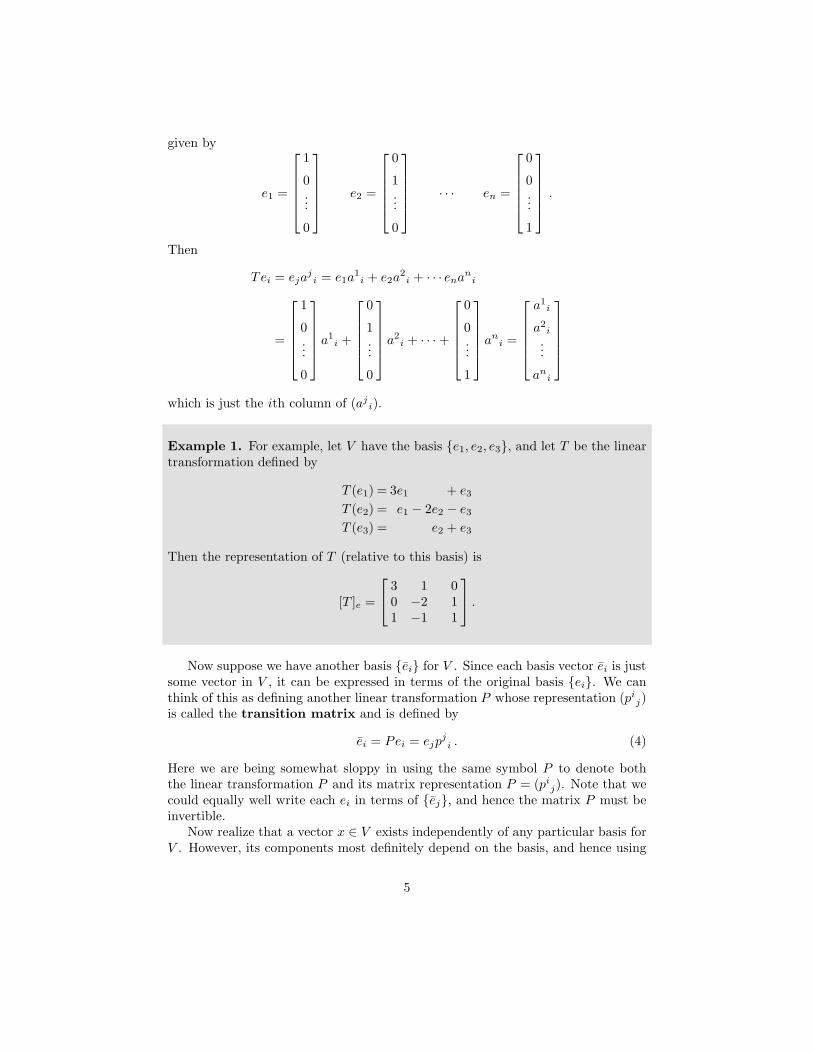
Example 1. For example, let V have the basis {e1, e2, e3}, and let T be the lineartransformation defined by

T (e1) = 3e1 + e3

T (e2) = e1 − 2e2 − e3

T (e3) = e2 + e3

Then the representation of T (relative to this basis) is

[T ]e =

3 1 00 −2 11 −1 1

.

Now suppose we have another basis {ei} for V . Since each basis vector ei is justsome vector in V , it can be expressed in terms of the original basis {ei}. We canthink of this as defining another linear transformation P whose representation (pi

j)is called the transition matrix and is defined by

ei = Pei = ejpji . (4)

Here we are being somewhat sloppy in using the same symbol P to denote boththe linear transformation P and its matrix representation P = (pi

j). Note that wecould equally well write each ei in terms of {ej}, and hence the matrix P must beinvertible.

Now realize that a vector x ∈ V exists independently of any particular basis forV . However, its components most definitely depend on the basis, and hence using

5

(4) we havex = xjej = xiei = xiejp

ji = (pj

ixi)ej .

Equating coefficients of each ej (this is an application of the uniqueness of theexpansion in terms of a given basis) we conclude that xj = pj

ixi or, equivalently,

xi = (p−1)ijx

j . (5)

Equations (4) and (5) describe the relationship between vector components withrespect to two distinct bases. What about the matrix representation of a lineartransformation T with respect to bases {ei} and {ei}? By definition we can writeboth

Tei = ejaji (6a)

and

T ei = ej aji . (6b)

Using (4) in the right side of (6b) we have

T ei = ekpkj a

ji

On the other hand, we can use (4) in the left side of (6b) and then use (6a) to write

T ei = T (ejpji) = pj

iTej = pjiekak

j = ekakjp

ji

where in the last step we wrote the matrix product in the correct order. Nowequate both forms of T ei and use the linear independence of the ek to conclude thatpk

j aji = ak

jpji which in matrix notation is just PA = AP . Since P is invertible

this can be written in the form that should be familiar to you:

A = P−1AP . (7)

A relationship of this form is called a similarity transformation. Be sure to notethat P goes from the basis {ei} to the basis {ei}.

Conversely, suppose T is represented by A in the basis {ei}, and let A = P−1AP .Defining a new basis {ei} by ei = Pei =

∑j ejpji it is straightforward to show that

the matrix representation of T relative to the basis {ei} is just A.

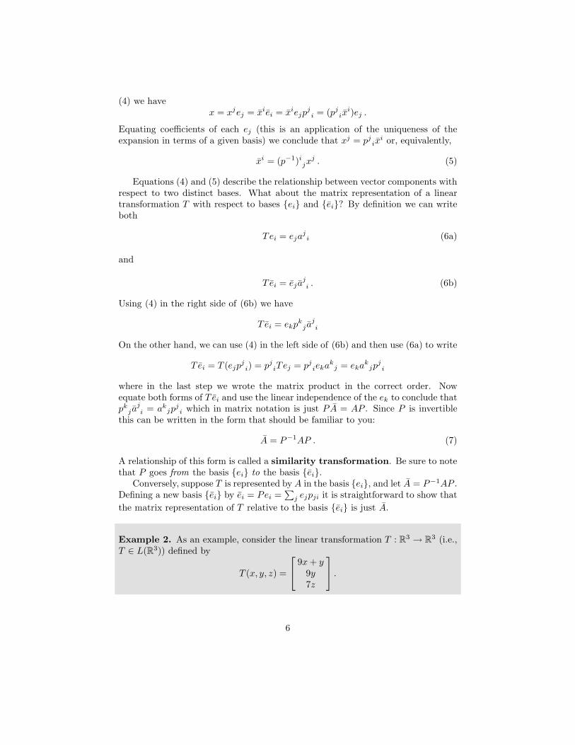
Example 2. As an example, consider the linear transformation T : R3 → R3 (i.e.,T ∈ L(R3)) defined by

T (x, y, z) =

9x + y9y7z

.

6

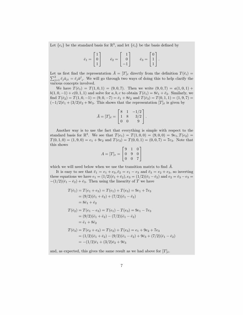
Let {ei} be the standard basis for R3, and let {ei} be the basis defined by

e1 =

101

e2 =

10

−1

e3 =

011

.

Let us first find the representation A = [T ]e directly from the definition T (ei) =∑3j=1 ejaji = eja

ji. We will go through two ways of doing this to help clarify the

various concepts involved.

We have T (e1) = T (1, 0, 1) = (9, 0, 7). Then we write (9, 0, 7) = a(1, 0, 1) +b(1, 0,−1) + c(0, 1, 1) and solve for a, b, c to obtain T (e1) = 8e1 + e2. Similarly, wefind T (e2) = T (1, 0,−1) = (9, 0,−7) = e1 + 8e2 and T (e3) = T (0, 1, 1) = (1, 9, 7) =(−1/2)e1 + (3/2)e2 + 9e3. This shows that the representation [T ]e is given by

A = [T ]e =

8 1 −1/21 8 3/20 0 9

.

Another way is to use the fact that everything is simple with respect to thestandard basis for R3. We see that T (e1) = T (1, 0, 0) = (9, 0, 0) = 9e1, T (e2) =T (0, 1, 0) = (1, 9, 0) = e1 + 9e2 and T (e3) = T (0, 0, 1) = (0, 0, 7) = 7e3. Note thatthis shows

A = [T ]e =

9 1 00 9 00 0 7

which we will need below when we use the transition matrix to find A.

It is easy to see that e1 = e1 + e3, e2 = e1 − e3 and e3 = e2 + e3, so invertingthese equations we have e1 = (1/2)(e1 + e2), e3 = (1/2)(e1 − e2) and e2 = e3 − e3 =−(1/2)(e1 − e2) + e3. Then using the linearity of T we have

T (e1) = T (e1 + e3) = T (e1) + T (e3) = 9e1 + 7e3

= (9/2)(e1 + e2) + (7/2)(e1 − e2)

= 8e1 + e2

T (e2) = T (e1 − e3) = T (e1) − T (e3) = 9e1 − 7e3

= (9/2)(e1 + e2) − (7/2)(e1 − e2)

= e1 + 8e2

T (e3) = T (e2 + e3) = T (e2) + T (e3) = e1 + 9e2 + 7e3

= (1/2)(e1 + e2) − (9/2)(e1 − e2) + 9e3 + (7/2)(e1 − e2)

= −(1/2)e1 + (3/2)e2 + 9e3

and, as expected, this gives the same result as we had above for [T ]e.

7

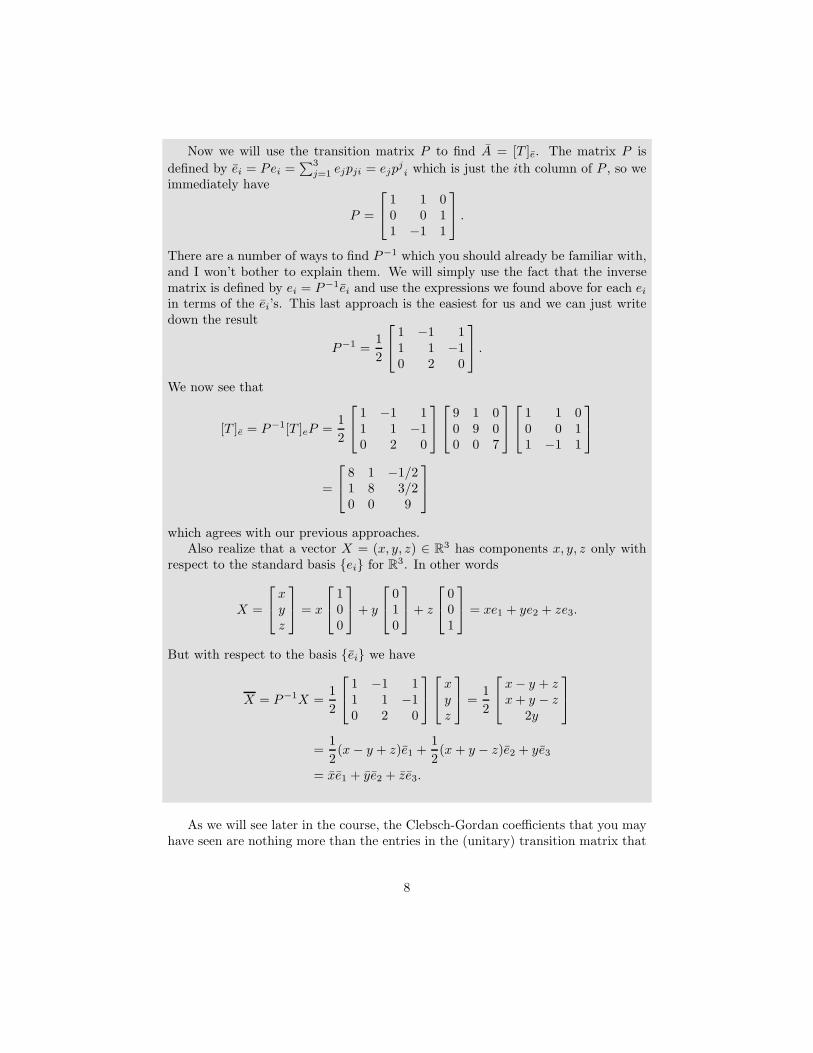
Now we will use the transition matrix P to find A = [T ]e. The matrix P is

defined by ei = Pei =∑3

j=1 ejpji = ejpji which is just the ith column of P , so we

immediately have

P =

1 1 00 0 11 −1 1

.

There are a number of ways to find P−1 which you should already be familiar with,and I won’t bother to explain them. We will simply use the fact that the inversematrix is defined by ei = P−1ei and use the expressions we found above for each ei

in terms of the ei’s. This last approach is the easiest for us and we can just writedown the result

P−1 =1

2

1 −1 11 1 −10 2 0

.

We now see that

[T ]e = P−1[T ]eP =1

2

1 −1 11 1 −10 2 0

9 1 00 9 00 0 7

1 1 00 0 11 −1 1

=

8 1 −1/21 8 3/20 0 9

which agrees with our previous approaches.Also realize that a vector X = (x, y, z) ∈ R3 has components x, y, z only with

respect to the standard basis {ei} for R3. In other words

X =

xyz

= x

100

+ y

010

+ z

001

= xe1 + ye2 + ze3.

But with respect to the basis {ei} we have

X = P−1X =1

2

1 −1 11 1 −10 2 0

xyz

=

1

2

x − y + zx + y − z

2y

=1

2(x − y + z)e1 +

1

2(x + y − z)e2 + ye3

= xe1 + ye2 + ze3.

As we will see later in the course, the Clebsch-Gordan coefficients that you mayhave seen are nothing more than the entries in the (unitary) transition matrix that

8

takes you between the |j1j2m1m2〉 basis and the |j1j2jm〉 basis in the vector spaceof two-particle angular momentum states.

If T ∈ L(V ) is a linear transformation, then the image of T is the set

Im T = {Tx : x ∈ V } .

It is also easy to see that Im T is a subspace of V . Furthermore, we define the rank

of T to be the numberrankT = dim(ImT ) .

By picking a basis for KerT and extending it to a basis for all of V , it is not hardto show that the following result holds, often called the rank theorem:

dim(ImT ) + dim(KerT ) = dim V . (8)

It can also be shown that the rank of a linear transformation T is equal tothe rank of any matrix representation of T (which is independent of similaritytransformations). This is a consequence of the fact that Tei is the ith column ofthe matrix representation of T , and the set of all such vectors Tei spans Im T .Then rankT is the number of linearly independent vectors Tei, which is also thedimension of the column space of [T ]. But the dimension of the row and columnspaces of a matrix are the same, and this is what is meant by the rank of a matrix.Thus rankT = rank[T ].

Note that if T is one-to-one, then KerT = {0} so that dimKerT = 0. It thenfollows from (8) that rank[T ] = rankT = dim(ImT ) = dimV = n so that [T ] isinvertible.

Another result we will need is the following.

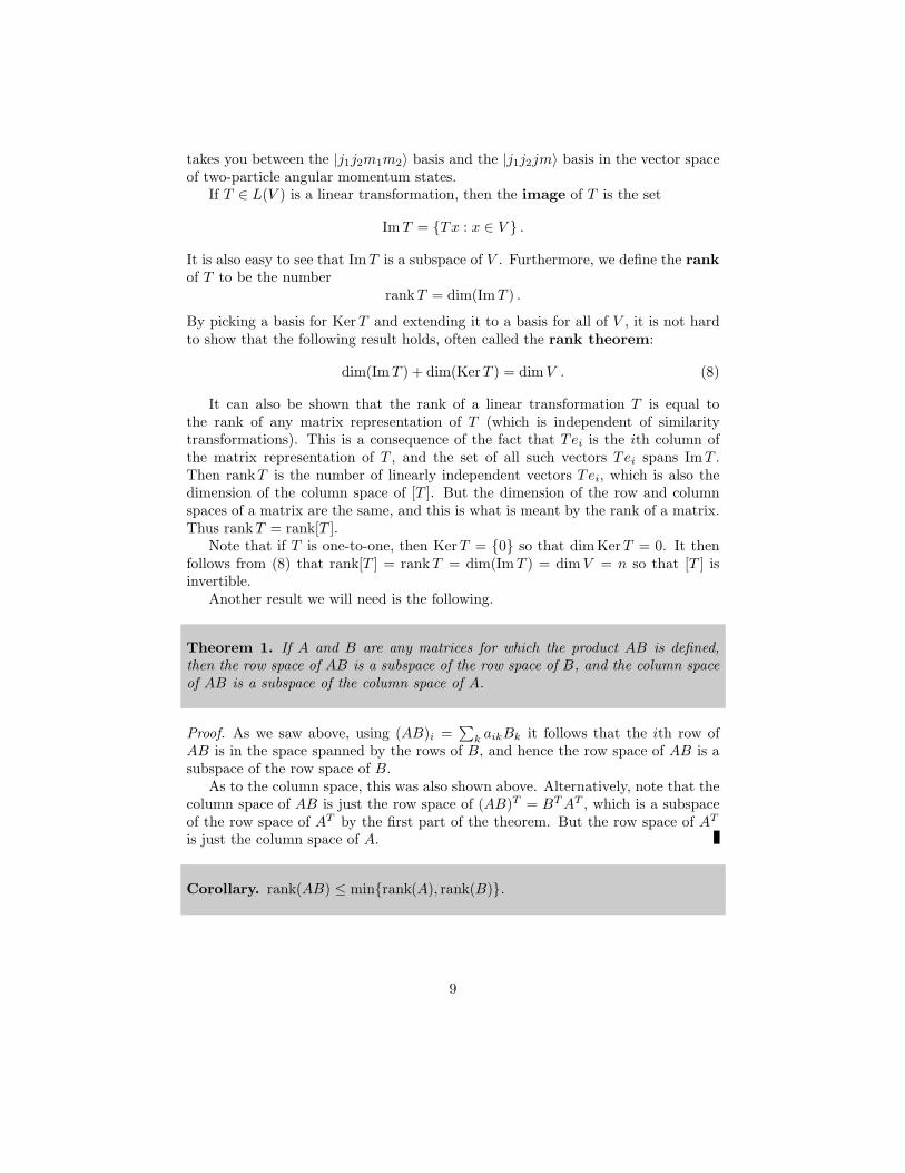
Theorem 1. If A and B are any matrices for which the product AB is defined,then the row space of AB is a subspace of the row space of B, and the column spaceof AB is a subspace of the column space of A.

Proof. As we saw above, using (AB)i =∑

k aikBk it follows that the ith row ofAB is in the space spanned by the rows of B, and hence the row space of AB is asubspace of the row space of B.

As to the column space, this was also shown above. Alternatively, note that thecolumn space of AB is just the row space of (AB)T = BT AT , which is a subspaceof the row space of AT by the first part of the theorem. But the row space of AT

is just the column space of A.

Corollary. rank(AB) ≤ min{rank(A), rank(B)}.

9

Proof. Let row(A) be the row space of A, and let col(A) be the column space of A.Then

rank(AB) = dim(row(AB)) ≤ dim(row(B)) = rank(B)

whilerank(AB) = dim(col(AB)) ≤ dim(col(A)) = rank(A).

The last topic I want to cover in this section is to briefly explain the mathematicsof two-particle states. While this isn’t really necessary for this course and we won’tdeal with it in detail, it should help you better understand what is going on whenwe add angular momenta. In addition, this material is necessary to understanddirect product representations of groups, which is quite important in its own right.

So, given two vector spaces V and V ′, we may define a bilinear map V × V ′ →V ⊗ V ′ that takes ordered pairs (v, v′) ∈ V × V ′ and gives a new vector denotedby v ⊗ v′. Since this map is bilinear by definition (meaning that it is linear in eachvariable separately), if we have the linear combinations v =

∑xivi and v′ =

∑yjv

′j

then v ⊗ v′ =∑

xiyj(vi ⊗ v′j). In particular, if V has basis {ei} and V ′ has basis{e′j}, then {ei⊗e′j} is a basis for V ⊗V ′ which is then of dimension (dim V )(dim V ′)and called the direct (or tensor) product of V and V ′.

If we are given two operators A ∈ L(V ) and B ∈ L(V ′), the direct product ofA and B is the operator A ⊗ B defined on V ⊗ V ′ by

(A ⊗ B)(v ⊗ v′) := A(v) ⊗ B(v′) .

We know that the matrix representation of an operator is defined by its values on abasis, and the ith basis vector goes to the ith column of the matrix representation.In the case of the direct product, we choose an ordered basis by taking all of the(dimV )(dim V ′) = mn elements ei ⊗ e′j in the obvious order

{e1 ⊗ e′1, . . . , e1 ⊗ e′n, e2 ⊗ e′1, . . . , e2 ⊗ e′n, . . . , em ⊗ e′1, . . . , em ⊗ e′n} .

Now our matrix elements are labeled by double subscripts because each basis vectoris labeled by two subscripts.

The (ij)th column of C = A ⊗ B is given in the usual way by acting on ei ⊗ e′jwith A ⊗ B:

(A ⊗ B)(ei ⊗ e′j) = Aei ⊗ Be′j = ekaki ⊗ e′lb

lj = (ek ⊗ e′l)a

kib

lj

= (ek ⊗ e′l)(A ⊗ B)klij .

For example, the (1, 1)th column of C is the vector (A⊗B)(e1⊗e′1) = ak1b

l1(ek⊗e′l)

given by

(a11b

11, . . . , a

11b

n1, a

21b

11, . . . , a

21b

n1, . . . , a

m1b

11, . . . , a

m1b

n1)

and in general, the (i, j)th column is given by

(a1ib

1j , . . . , a

1ib

nj , a

2ib

1j , . . . , a

2ib

nj , . . . , a

mib

1j , . . . , a

mib

nj) .

10

If we write this as the column vector it is,

a1ib

1j

...a1

ibn

j

...

amib

1j

...am

ibn

j

then it is not hard to see this shows that the matrix C has the block matrix form

C =

a11B a1

2B · · · a1mB

......

...

am1B am

2B · · · ammB

.

As I said, we will see an application of this formalism when we treat the additionof angular momentum.

2 The Levi-Civita Symbol and the Vector Cross

Product

In order to ease into the notation we will use, we begin with an elementary treatmentof the vector cross product. This will give us a very useful computational tool thatis of importance in and of itself. While you are probably already familiar with thecross product, we will still go through its development from scratch just for the sakeof completeness.

To begin with, consider two vectors a and b in R3 (with Cartesian coordinates).There are two ways to define their vector product (or cross product) a × b.The first way is to define a × b as that vector with norm given by

‖a× b‖ = ‖a‖ ‖b‖ sin θ

where θ is the angle between a and b, and whose direction is such that the triple(a,b,a×b) has the same “orientation” as the standard basis vectors (x, y, z). Thisis commonly referred to as “the right hand rule.” In other words, if you rotate a

into b thru the smallest angle between them with your right hand as if you wereusing a screwdriver, then the screwdriver points in the direction of a×b. Note thatby definition, a × b is perpendicular to the plane spanned by a and b.

The second way to define a×b is in terms of its vector components. I will startfrom this definition and show that it is in fact equivalent to the first definition. So,

11

we define a × b to be the vector c with components

cx = (a × b)x = aybz − azby

cy = (a × b)y = azbx − axbz

cz = (a × b)z = axby − aybx

Before proceeding, note that instead of labeling components by (x, y, z) it willbe very convenient for us to use (x1, x2, x3). This is standard practice, and it willgreatly facilitate many equations throughout the remainder of these notes. Usingthis notation, the above equations are written

c1 = (a × b)1 = a2b3 − a3b2

c2 = (a × b)2 = a3b1 − a1b3

c3 = (a × b)3 = a1b2 − a2b1

We now see that each equation can be obtained from the previous by cyclicallypermuting the subscripts 1 → 2 → 3 → 1.

Using these equations, it is easy to multiply out components and verify thata · c = a1c1 + a2c2 + a3c3 = 0, and similarly b · c = 0. This shows that a × b isperpendicular to both a and b, in agreement with our first definition.

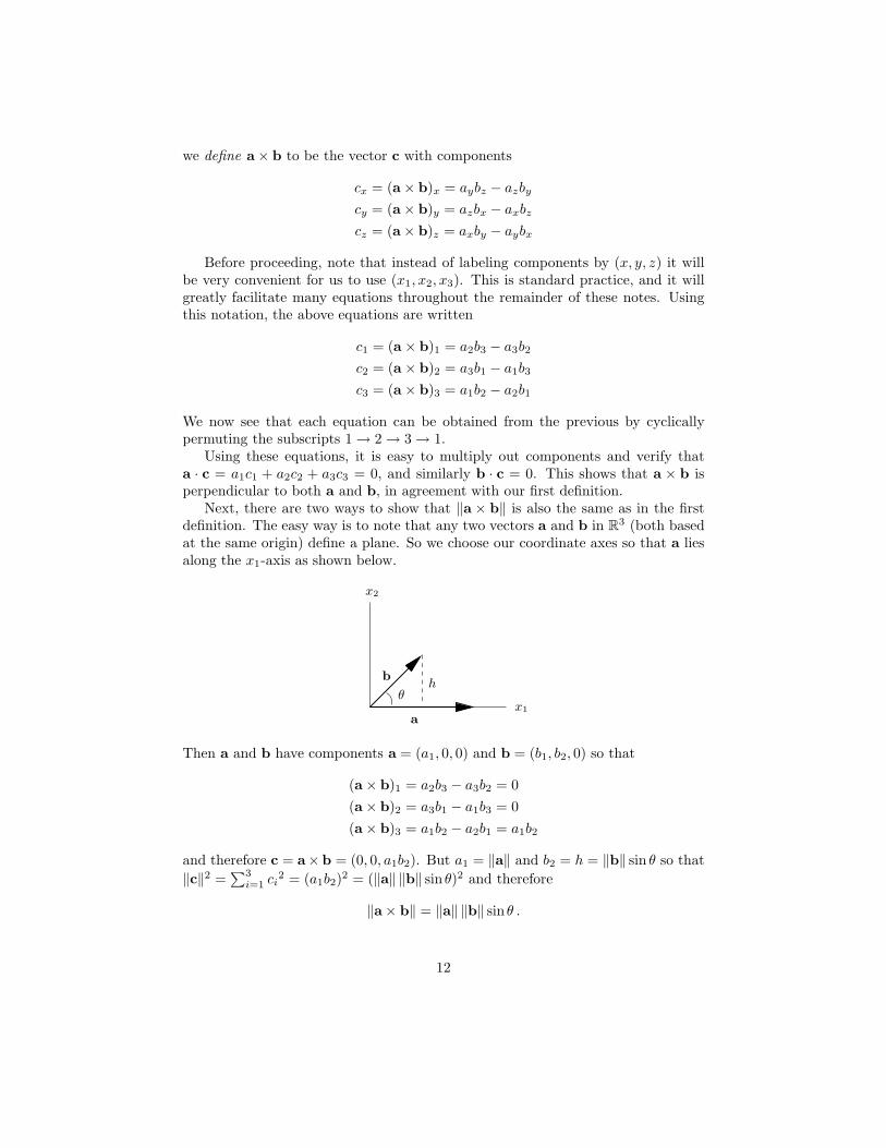
Next, there are two ways to show that ‖a × b‖ is also the same as in the firstdefinition. The easy way is to note that any two vectors a and b in R3 (both basedat the same origin) define a plane. So we choose our coordinate axes so that a liesalong the x1-axis as shown below.

x1

x2

h

a

b

θ

Then a and b have components a = (a1, 0, 0) and b = (b1, b2, 0) so that

(a × b)1 = a2b3 − a3b2 = 0

(a × b)2 = a3b1 − a1b3 = 0

(a × b)3 = a1b2 − a2b1 = a1b2

and therefore c = a×b = (0, 0, a1b2). But a1 = ‖a‖ and b2 = h = ‖b‖ sin θ so that

‖c‖2 =∑3

i=1 ci2 = (a1b2)

2 = (‖a‖ ‖b‖ sin θ)2 and therefore

‖a× b‖ = ‖a‖ ‖b‖ sin θ .

12

Since both the length of a vector and the angle between two vectors is independentof the orientation of the coordinate axes, this result holds for arbitrary a and b.Therefore ‖a × b‖ is the same as in our first definition.

The second way to see this is with a very unenlightening brute force calculation:

‖a× b‖2 = (a × b) · (a × b) = (a × b)12

+ (a × b)22

+ (a × b)32

= (a2b3 − a3b2)2 + (a3b1 − a1b3)

2 + (a1b2 − a2b1)2

= a22b3

2 + a32b2

2 + a32b1

2 + a12b3

2 + a12b2

2 + a22b1

2

− 2(a2b3a3b2 + a3b1a1b3 + a1b2a2b1)

= (a22 + a3

2)b12 + (a1

2 + a32)b2

2 + (a12 + a2

2)b32

− 2(a2b2a3b3 + a1b1a3b3 + a1b1a2b2)

= (add and subtract terms)

= (a12 + a2

2 + a32)b1

2 + (a12 + a2

2 + a32)b2

2

+ (a12 + a2

2 + a32)b3

2 − (a12b1

2 + a22b2

2 + a32b3

2)

− 2(a2b2a3b3 + a1b1a3b3 + a1b1a2b2)

= (a12 + a2

2 + a32)(b1

2 + b22 + b3

2) − (a1b1 + a2b2 + a3b3)2

= ‖a‖2 ‖b‖2 − (a · b)2 = ‖a‖2 ‖b‖2 − ‖a‖2 ‖b‖2 cos2 θ

= ‖a‖2 ‖b‖2(1 − cos2 θ) = ‖a‖2 ‖b‖2 sin2 θ

so again we have ‖a× b‖ = ‖a‖ ‖b‖ sin θ.To see the geometrical meaning of the vector product, first take a look at the

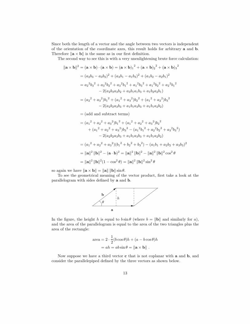
parallelogram with sides defined by a and b.

a

b

θh

In the figure, the height h is equal to b sin θ (where b = ‖b‖ and similarly for a),and the area of the parallelogram is equal to the area of the two triangles plus thearea of the rectangle:

area = 2 · 1

2(b cos θ)h + (a − b cos θ)h

= ah = ab sin θ = ‖a× b‖ .

Now suppose we have a third vector c that is not coplanar with a and b, andconsider the parallelepiped defined by the three vectors as shown below.

13

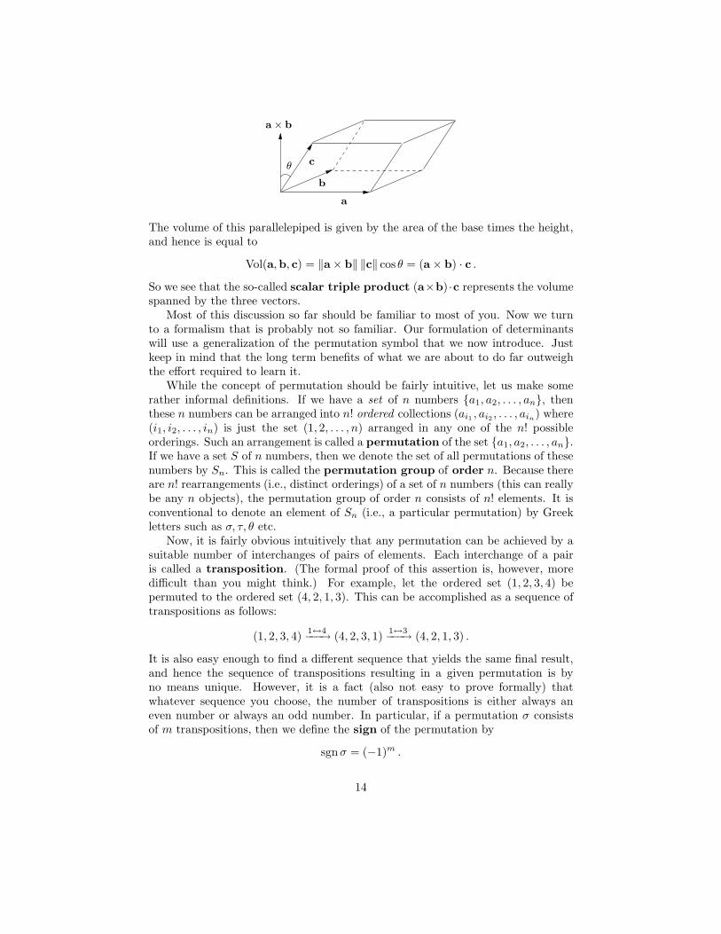
a

b

c

a× b

θ

The volume of this parallelepiped is given by the area of the base times the height,and hence is equal to

Vol(a,b, c) = ‖a× b‖ ‖c‖ cos θ = (a × b) · c .

So we see that the so-called scalar triple product (a×b) ·c represents the volumespanned by the three vectors.

Most of this discussion so far should be familiar to most of you. Now we turnto a formalism that is probably not so familiar. Our formulation of determinantswill use a generalization of the permutation symbol that we now introduce. Justkeep in mind that the long term benefits of what we are about to do far outweighthe effort required to learn it.

While the concept of permutation should be fairly intuitive, let us make somerather informal definitions. If we have a set of n numbers {a1, a2, . . . , an}, thenthese n numbers can be arranged into n! ordered collections (ai1 , ai2 , . . . , ain

) where(i1, i2, . . . , in) is just the set (1, 2, . . . , n) arranged in any one of the n! possibleorderings. Such an arrangement is called a permutation of the set {a1, a2, . . . , an}.If we have a set S of n numbers, then we denote the set of all permutations of thesenumbers by Sn. This is called the permutation group of order n. Because thereare n! rearrangements (i.e., distinct orderings) of a set of n numbers (this can reallybe any n objects), the permutation group of order n consists of n! elements. It isconventional to denote an element of Sn (i.e., a particular permutation) by Greekletters such as σ, τ, θ etc.

Now, it is fairly obvious intuitively that any permutation can be achieved by asuitable number of interchanges of pairs of elements. Each interchange of a pairis called a transposition. (The formal proof of this assertion is, however, moredifficult than you might think.) For example, let the ordered set (1, 2, 3, 4) bepermuted to the ordered set (4, 2, 1, 3). This can be accomplished as a sequence oftranspositions as follows:

(1, 2, 3, 4)1↔4−−−→ (4, 2, 3, 1)

1↔3−−−→ (4, 2, 1, 3) .

It is also easy enough to find a different sequence that yields the same final result,and hence the sequence of transpositions resulting in a given permutation is byno means unique. However, it is a fact (also not easy to prove formally) thatwhatever sequence you choose, the number of transpositions is either always aneven number or always an odd number. In particular, if a permutation σ consistsof m transpositions, then we define the sign of the permutation by

sgnσ = (−1)m .

14

Because of this, it makes sense to talk about a permutation as being either even

(if m is even) or odd (if m is odd).Now that we have a feeling for what it means to talk about an even or an odd

permutation, let us define the Levi-Civita symbol εijk (also frequently referredto as the permutation symbol) by

εijk =

1 if (i, j, k) is an even permutation of (1, 2, 3)

−1 if (i, j, k) is an odd permutation of (1, 2, 3)

0 if (i, j, k) is not a permutation of (1, 2, 3)

.

In other words,

ε123 = −ε132 = ε312 = −ε321 = ε231 = −ε213 = 1

and εijk = 0 if there are any repeated indices. We also say that εijk is antisym-

metric in all three indices, meaning that it changes sign upon interchanging anytwo indices. For a given order (i, j, k) the resulting number εijk is also called thesign of the permutation.

Before delving further into some of the properties of the Levi-Civita symbol,let’s take a brief look at how it is used. Given two vectors a and b, we can let i = 1and form the double sum

∑3j,k=1 ε1jkajbk. Since εijk = 0 if any two indices are

repeated, the only possible values for j and k are 2 and 3. Then

3∑

j,k=1

ε1jkajbk = ε123a2b3 + ε132a3b2 = a2b3 − a3b2 = (a × b)1 .

But the components of the cross product are cyclic permutations of each other,and εijk doesn’t change sign under cyclic permutations, so we have the importantgeneral result

(a × b)i =

3∑

j,k=1

εijkajbk . (9)

(A cyclic permutation is one of the form 1 → 2 → 3 → 1 or x → y → z → x.)Now, in order to handle various vector identities, we need to prove some other

properties of the Levi-Civita symbol. The first identity to prove is this:

3∑

i,j,k=1

εijkεijk = 3! = 6 . (10)

But this is actually easy, because (i, j, k) must all be different, and there are 3!ways to order (1, 2, 3). In other words, there are 3! permutations of {1, 2, 3}. Forevery case where all three indices are different, whether εijk is +1 or −1, we alwayshave (εijk)2 = +1, and therefore summing over the 3! possibilities yields the desiredresult.

15

Recalling the Einstein summation convention, it is important to keep the place-ment of any free (i.e., unsummed over) indices the same on both sides of an equa-tion. For example, we would always write something like AijB

jk = Cik and not

AijBjk = Cik. In particular, the ith component of the cross product is written

(a × b)i = εijkajbk . (11)

As mentioned earlier, for our present purposes, raising and lowering an index ispurely a notational convenience. And in order to maintain the proper index place-ment, we will frequently move an index up or down as necessary. While this mayseem quite confusing at first, with a little practice it becomes second nature andresults in vastly simplified calculations.

Using this convention, equation (10) is simply written εijkεijk = 6. This also

applies to the Kronecker delta, so that we have expressions like aiδji =

∑3i=1 aiδj

i =

aj (where δji is numerically the same as δij). An inhomogeneous system of linear

equations would be written as simply aijx

j = yi, and the dot product as

a · b = aibi = aibi . (12)

Note also that indices that are summed over are “dummy indices” meaning, forexample, that aib

i = akbk. This is simply another way of writing∑3

i=1 aibi =

a1b1 + a2b2 + a3b3 =∑3

k=1 akbk.As we have said, the Levi-Civita symbol greatly simplifies many calculations

dealing with vectors. Let’s look at some examples.

Example 3. Let us take a look at the scalar triple product. We have

a · (b × c) = ai(b × c)i = aiεijkbjck

= bjεjkickai (because εijk = −εjik = +εjki)

= bj(c × a)j

= b · (c × a) .

Note also that this formalism automatically takes into account the anti-symmetryof the cross product:

(c × a)i = εijkcjak = −εikjcjak = −εikja

kcj = −(a× c)i .

It doesn’t get any easier than this.

Of course, this formalism works equally well with vector calculus equations in-volving the gradient ∇. This is the vector defined by

∇ = x∂

∂x+ y

∂

∂y+ z

∂

∂z= x1

∂

∂x1+ x2

∂

∂x2+ x3

∂

∂x3= ei ∂

∂xi.

16

In fact, it will also be convenient to simplify our notation further by defining ∇i =∂/∂xi = ∂i, so that ∇ = ei∂i.

Example 4. Let us prove the well-known identity ∇ · (∇× a) = 0. We have

∇ · (∇× a) = ∇i(∇× a)i = ∂i(εijk∂jak) = εijk∂i∂jak .

But now notice that εijk is antisymmetric in i and j (so that εijk = −εjik), whilethe product ∂i∂j is symmetric in i and j (because we assume that the order ofdifferentiation can be interchanged so that ∂i∂j = ∂j∂i). Then

εijk∂i∂j = −εjik∂i∂j = −εjik∂j∂i = −εijk∂i∂j

where the last step follows because i and j are dummy indices, and we can thereforerelabel them. But then εijk∂i∂j = 0 and we have proved our identity.

The last step in the previous example is actually a special case of a generalresult. To see this, suppose that we have an object Aij··· that is labeled by two ormore indices, and suppose that it is antisymmetric in two of those indices (say i, j).This means that Aij··· = −Aji···. Now suppose that we have another object Sij···

that is symmetric in i and j, so that Sij··· = Sji···. If we multiply A times S andsum over the indices i and j, then using the symmetry and antisymmetry propertiesof S and A we have

Aij···Sij··· = −Aji···Sij··· by the antisymmetry of A

= −Aji···Sji··· by the symmetry of S

= −Aij···Sij··· by relabeling the dummy indices i and j

and therefore we have the general result

Aij···Sij··· = 0 .

It is also worth pointing out that the indices i and j need not be the first pair of in-dices, nor do they need to be adjacent. For example, we still have A···i···j···S···i···j··· =0.

Now suppose that we have an arbitrary object T ij without any particular sym-metry properties. Then we can turn this into an antisymmetric object T [ij] by aprocess called antisymmetrization as follows:

T ij → T [ij] :=1

2!(T ij − T ji) .

In other words, we add up all possible permutations of the indices, with the signof each permutation being either +1 (for an even permutation) or −1 (for an odd

17

permutation), and then divide this sum by the total number of permutations, whichin this case is 2!. If we have something of the form T ijk then we would have

T ijk → T [ijk] :=1

3!(T ijk − T ikj + T kij − T kji + T jki − T jik)

where we alternate signs with each transposition. The generalization to an arbitrarynumber of indices should be clear. Note also that we could antisymmetrize onlyover a subset of the indices if required.

It is also important to note that it is impossible to have a nonzero antisymmetricobject with more indices than the dimension of the space we are working in. Thisis simply because at least one index will necessarily be repeated. For example, if weare in R3, then anything of the form T ijkl must have at least one index repeatedbecause each index can only range between 1, 2 and 3.

Now, why did we go through all of this? Well, first recall that we can writethe Kronecker delta in any of the equivalent forms δij = δi

j = δji . Then we can

construct quantities like

δ[1i δ

2]j =

1

2!

(δ1i δ2

j − δ2i δ1

j

)= δ1

[iδ2j]

and

δ[1i δ

2j δ

3]k =

1

3!

(δ1i δ2

j δ3k − δ1

i δ3j δ2

k + δ3i δ1

j δ2k − δ3

i δ2j δ1

k + δ2i δ3

j δ1k − δ2

i δ1j δ3

k

).

In particular, we now want to show that

εijk = 3! δ[1i δ

2j δ

3]k . (13)

Clearly, if i = 1, j = 2 and k = 3 we have

3! δ[11 δ

22 δ

3]3 = 3!

1

3!

(δ11δ

22δ

33 − δ1

1δ32δ2

3 + δ31δ1

2δ23 − δ3

1δ22δ

13 + δ2

1δ32δ1

3 − δ21δ1

2δ33

)

= 1 − 0 + 0 − 0 + 0 − 0 = 1 = ε123

so equation (13) is correct in this particular case. But now we make the crucialobservation that both sides of equation (13) are antisymmetric in (i, j, k), and hencethe equation must hold for all values of (i, j, k). This is because any permutation of(i, j, k) results in the same change of sign on both sides, and both sides also equal0 if any two indices are repeated. Therefore equation (13) is true in general.

To derive what is probably the most useful identity involving the Levi-Civitasymbol, we begin with the fact that ε123 = 1. Multiplying the left side of equation(13) by 1 in this form yields

εijk ε123 = 3! δ[1i δ

2j δ

3]k .

But now we again make the observation that both sides are antisymmetric in(1, 2, 3), and hence both sides are equal for all values of the upper indices, andwe have the fundamental result

εijk εnlm = 3! δ[ni δ

lj δ

m]k . (14)

18

We now set n = k and sum over k. (This process of setting two indices equal toeach other and summing is called contraction.) Using the fact that

δkk =

3∑

i=1

δkk = 3

along with terms such as δki δm

k = δmi we find

εijk εklm = 3! δ[ki δ

lj δ

m]k

= δki δl

jδmk − δk

i δmj δl

k + δmi δk

j δlk − δm

i δljδ

kk + δl

iδmj δk

k − δliδ

kj δm

k

= δmi δl

j − δliδ

mj + δm

i δlj − 3δm

i δlj + 3δl

iδmj − δl

iδmj

= δliδ

mj − δm

i δlj .

In other words, we have the extremely useful result

εijk εklm = δliδ

mj − δm

i δlj . (15)

This result is so useful that it should definitely be memorized.

Example 5. Let us derive the well-known triple vector product known as the“bac− cab” rule. We simply compute using equation (15):

[a× (b × c)]i = εijkaj(b × c)k = εijkεklmajblcm

= (δliδ

mj − δm

i δlj)a

jblcm = ambicm − ajbjci

= bi(a · c) − ci(a · b)

and thereforea × (b × c) = b(a · c) − c(a · b) .

We also point out that some of the sums in this derivation can be done in morethan one way. For example, we have either δl

iδmj ajblcm = ambicm = bi(a · c) or

δliδ

mj ajblcm = ajbicj = bi(a · c), but the end result is always the same. Note also

that at every step along the way, the only index that isn’t repeated (and hencesummed over) is i.

Example 6. Equation (15) is just as useful in vector calculus calculations. Here isan example to illustrate the technique.

[∇× (∇× a)]i = εijk∂j(∇× a)k = εijkεklm∂j∂lam

= (δliδ

mj − δm

i δlj)∂

j∂lam = ∂j∂iaj − ∂j∂jai

= ∂i(∇ · a) −∇2ai

19

and hence we have the identity

∇× (∇× a) = ∇(∇ · a) −∇2a

which is very useful in discussing the theory of electromagnetic waves.

3 Determinants

In treating vectors in R3, we used the permutation symbol εijk defined in the

last section. We are now ready to apply the same techniques to the theory ofdeterminants. The idea is that we want to define a mapping from a matrix A ∈Mn(F) to F in a way that has certain algebraic properties. Since a matrix inMn(F) has components aij with i and j ranging from 1 to n, we are going to needa higher dimensional version of the Levi-Civita symbol already introduced. Theobvious extension to n dimensions is the following.

We define

εi1··· in =

1 if i1, . . . , in is an even permutation of 1, . . . , n

−1 if i1, . . . , in is an odd permutation of 1, . . . , n

0 if i1, . . . , in is not a permutation of 1, . . . , n

.

Again, there is no practical difference between εi1··· in and εi1··· in. Using this, we

define the determinant of A = (aij) ∈ Mn(F) to be the number

detA = εi1··· ina1i1a2i2 · · · anin. (16)

Look carefully at what this expression consists of. Since εi1··· in vanishes unless(i1, . . . , in) are all distinct, and there are n! such distinct orderings, we see thatdetA consists of n! terms in the sum, where each term is a product of n factors aij ,and where each term consists precisely of one factor from each row and each columnof A. In other words, detA is a sum of terms where each term is a product of oneelement from each row and each column, and the sum is over all such possibilities.

The determinant is frequently written as

detA =

∣∣∣∣∣∣∣

a11 . . . a1n

......

an1 . . . ann

∣∣∣∣∣∣∣.

The determinant of an n × n matrix is said to be of order n. Note also that thedeterminant is only defined for square matrices.

20

Example 7. Leaving the easier 2 × 2 case to you to verify, we will work out the3 × 3 case and show that it gives the same result that you probably learned in amore elementary course. So, for A = (aij) ∈ M3(F) we have

detA = εijka1ia2ja3k

= ε123a11a22a33 + ε132a11a23a32 + ε312a13a21a32

+ ε321a13a22a31 + ε231a12a23a31 + ε213a12a21a33

= a11a22a33 − a11a23a32 + a13a21a32

− a13a22a31 + a12a23a31 − a12a21a33

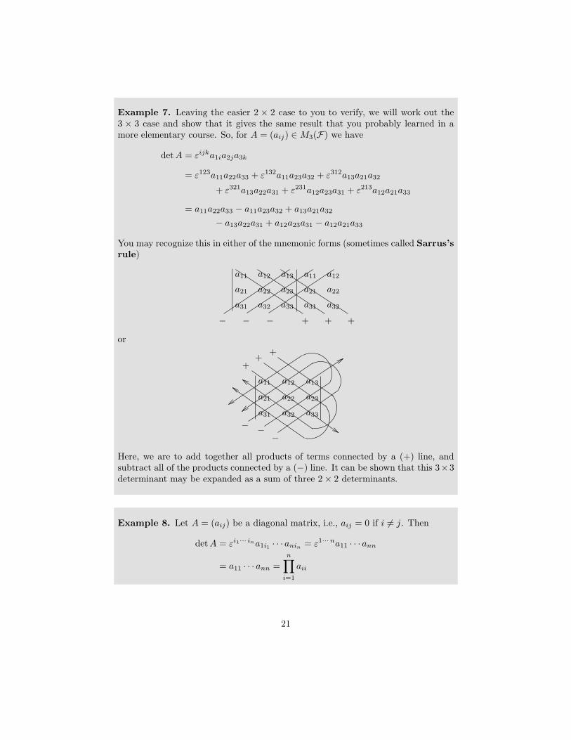
You may recognize this in either of the mnemonic forms (sometimes called Sarrus’s

rule)

a11a11 a12a12 a13

a21a21 a22a22 a23

a31a31 a32a32 a33

− −− ++ +

or

a11 a12 a13

a21 a22 a23

a31 a32 a33

− −−

+

++

Here, we are to add together all products of terms connected by a (+) line, andsubtract all of the products connected by a (−) line. It can be shown that this 3×3determinant may be expanded as a sum of three 2 × 2 determinants.

Example 8. Let A = (aij) be a diagonal matrix, i.e., aij = 0 if i 6= j. Then

detA = εi1··· ina1i1 · · ·anin= ε1···na11 · · · ann

= a11 · · · ann =

n∏

i=1

aii

21

so that ∣∣∣∣∣∣∣

a11 · · · 0...

. . ....

0 · · · ann

∣∣∣∣∣∣∣=

n∏

i=1

aii .

In particular, we see that det I = 1.

We now prove a number of useful properties of determinants. These are all verystraightforward applications of the definition (16) once you have become comfortablewith the notation. In fact, in my opinion, this approach to determinants affords thesimplest way in which to arrive at these results, and is far less confusing than theusual inductive proofs.

Theorem 2. For any A ∈ Mn(F) we have

detA = detAT .

Proof. This is simply an immediate consequence of our definition of determinant.We saw that detA is a sum of all possible products of one element from each rowand each column, and no product can contain more than one term from a givencolumn because the corresponding ε symbol would vanish. This means that anequivalent way of writing all n! such products is (note the order of subscripts isreversed)

det A = εi1··· inai11 · · ·ainn .

But aij = aTji so this is just

detA = εi1··· inai11 · · ·ainn = εi1··· inaT1i1 · · · aT

nin= detAT .

In order to help us gain some additional practice manipulating these quantities,we prove this theorem again based on another result which we will find very usefulin its own right. We start from the definition det A = εi1··· ina1i1 · · · anin

. Againusing ε1···n = 1 we have

ε1···n detA = εi1··· ina1i1 · · · anin. (17)

By definition of the permutation symbol, the left side of this equation is antisym-metric in (1, . . . , n). But so is the right side because, taking a1i1 and a2i2 as anexample, we see that

εi1i2··· ina1i1a2i2 · · · anin= εi1i2··· ina2i2a1i1 · · · anin

= −εi2i1··· ina2i2a1i1 · · · anin

= −εi1i2··· ina2i1a1i2 · · · anin

22

where the last line follows by a relabeling of the dummy indices i1 and i2.So, by a now familiar argument, both sides of equation (17) must be true for

any values of the indices (1, . . . , n) and we have the extremely useful result

εj1··· jndetA = εi1··· inaj1i1 · · · ajnin

. (18)

This equation will turn out to be very helpful in many proofs that would otherwisebe considerably more difficult.

Let us now use equation (18) to prove Theorem 2. We begin with the analogousresult to equation (10). This is

εi1··· inεi1··· in= n!. (19)

Using this, we multiply equation (18) by εj1··· jn to yield

n! detA = εj1··· jnεi1··· inaj1i1 · · ·ajnin.

On the other hand, by definition of detAT we have

det AT = εi1··· inaT1i1 · · · aT

nin= εi1··· inai11 · · ·ainn .

Multiplying the left side of this equation by 1 = ε1···n and again using the antisym-metry of both sides in (1, . . . , n) yields

εj1··· jndetAT = εi1··· inai1j1 · · · ajnin

.

(This also follows by applying equation (18) to AT directly.)Now multiply this last equation by εj1··· jn to obtain

n! detAT = εi1··· inεj1··· jnai1j1 · · · ajnin.

Relabeling the dummy indices i and j we have

n! detAT = εj1··· jnεi1··· inaj1i1 · · · ainjn

which is exactly the same as the above expression for n! detA, and we have againproved Theorem 2.

Let us restate equation (18) as a theorem for emphasis, and also look at two ofits immmediate consequences.

Theorem 3. If A ∈ Mn(F), then

εj1··· jndetA = εi1··· inaj1i1 · · · ajnin

.

23

Corollary 1. If B ∈ Mn(F) is obtained from A ∈ Mn(F) by interchanging tworows of A, the detB = − detA.

Proof. This is really just what the theorem says in words. (See the discussionbetween equations (17) and (18).) For example, let B result from interchangingrows 1 and 2 of A. Then

detB = εi1i2··· inb1i1b2i2 · · · bnin= εi1i2··· ina2i1a1i2 · · · anin

= εi1i2··· ina1i2a2i1 · · · anin= −εi2i1··· ina1i2a2i1 · · · anin

= −εi1i2··· ina1i1a2i2 · · · anin

= − detA = ε213···n detA .

where again the next to last line follows by relabeling.

Corollary 2. If A ∈ Mn(F) has two identical rows, then detA = 0.

Proof. If B is the matrix obtained by interchanging two identical rows of A, thenby the previous corollary we have

detA = detB = − detA

and therefore detA = 0.

Here is another way to view Theorem 3 and its corollaries. If we view detA asa function of the rows of A, then the corollaries state that det A = 0 if any tworows are the same, and detA changes sign if two nonzero rows are interchanged. Inother words, we have

det(Aj1 , . . . , Ajn) = εj1··· jn

det A . (20)

If it isn’t immediately obvious to you that this is true, then note that for (j1, . . . , jn) =(1, . . . , n) it’s just an identity. So by the antisymmetry of both sides, it must betrue for all j1, . . . , jn.

Looking at the definition detA = εi1··· ina1i1 · · · anin, we see that we can view

the determinant as a function of the rows of A: det A = det(A1, . . . , An). Sinceeach row is actually a vector in Fn, we can replace A1 (for example) by any linearcombination of two vectors in Fn so that A1 = rB1 + sC1 where r, s ∈ F andB1, C1 ∈ Fn. Let B = (bij) be the matrix with rows Bi = Ai for i = 2, . . . , n, andlet C = (cij) be the matrix with rows Ci = Ai for i = 2, . . . , n. Then

detA = det(A1, A2, . . . , An) = det(rB1 + sC1, A2, . . . , An)

= εi1··· in(rb1i1 + sc1i1)a2i2 · · · anin

= rεi1··· inb1i1a2i2 · · · anin+ sεi1··· inc1i1a2i2 · · · anin

= r detB + s detC.

24

Since this argument clearly could have been applied to any of the rows of A, wehave proved the following theorem.

Theorem 4. Let A ∈ Mn(F) have row vectors A1, . . . , An and assume that forsome i = 1, . . . , n we have

Ai = rBi + sCi

where Bi, Ci ∈ Fn and r, s ∈ F . Let B ∈ Mn(F) haverows A1, . . . , Ai−1, Bi, Ai+1, . . . , An and C ∈ Mn(F) have rowsA1, . . . , Ai−1, Ci, Ai+1, . . . , An. Then

det A = r detB + s detC.

Besides the very easy to handle diagonal matrices, another type of matrix thatis easy to deal with are the triangular matrices. To be precise, a matrix A ∈ Mn(F)is said to be upper-triangular if aij = 0 for i > j, and A is said to be lower-

triangular if aij = 0 for i < j. Thus a matrix is upper-triangular if it is of theform

a11 a12 a13 · · · a1n

0 a22 a23 · · · a2n

0 0 a33 · · · a3n

......

......

0 0 0 · · · ann

and lower-triangular if it is of the form

a11 0 0 · · · 0a21 a22 0 · · · 0a31 a32 a33 · · · 0...

......

...an1 an2 an3 · · · ann

.

We will use the term triangular to mean either upper- or lower-triangular.

Theorem 5. If A ∈ Mn(F) is a triangular matrix, then

detA =

n∏

i=1

aii.

Proof. If A is lower-triangular, then A is of the form shown above. Now lookcarefully at the definition detA = εi1··· ina1i1 · · · anin

. Since A is lower-triangularwe have aij = 0 for i < j. But then we must have i1 = 1 or else a1i1 = 0. Now

25

consider a2i2 . Since i1 = 1 and a2i2 = 0 if 2 < i2, we must have i2 = 2. Next, i1 = 1and i2 = 2 means that i3 = 3 or else a3i3 = 0. Continuing in this way we see thatthe only nonzero term in the sum is when ij = j for each j = 1, . . . , n and hence

detA = ε12 ···n a11 · · · ann =

n∏

i=1

aii.

If A is an upper-triangular matrix, then the theorem follows from Theorem 2.

An obvious corollary is the following (which was also shown directly in Example8).

Corollary. If A ∈ Mn(F) is diagonal, then detA =∏n

i=1 aii.

It is important to realize that because detAT = detA, Theorem 3 and itscorollaries apply to columns as well as to rows. Furthermore, these results nowallow us easily see what happens to the determinant of a matrix A when we applyelementary row (or column) operations to A. In fact, if you think for a moment,the answer should be obvious. For a type α transformation (i.e., interchanging tworows), we have just seen that detA changes sign (Theorem 3, Corollary 1). Fora type β transformation (i.e., multiply a single row by a nonzero scalar), we canlet r = k, s = 0 and Bi = Ai in Theorem 4 to see that det A → k detA. And fora type γ transformation (i.e., add a multiple of one row to another) we have (forAi → Ai + kAj and using Theorems 4 and 3, Corollary 2)

det(A1, . . . , Ai + kAj , . . . , An) = detA + k det(A1, . . . , Aj , . . . , Aj , . . . , An)

= detA + 0 = detA.

Summarizing these results, we have the following theorem.

Theorem 6. Suppose A ∈ Mn(F) and let B ∈ Mn(F) be row equivalent to A.(i) If B results from the interchange of two rows of A, then detB = − detA.(ii) If B results from multiplying any row (or column) of A by a scalar k, then

detB = k detA.(iii) If B results from adding a multiple of one row of A to another row, then

detB = detA.

Corollary. If R is the reduced row-echelon form of a matrix A, then detR = 0 ifand only if detA = 0.

Proof. This follows from Theorem 6 since A and R are row-equivalent.

26

Now, A ∈ Mn(F) is singular if rankA < n. Hence there must be at least onezero row in the reduced row echelon form R of A, and thus detA = detR = 0.Conversely, if rankA = n, then the reduced row echelon form R of A is just I, andhence detR = 1 6= 0. Therefore detA 6= 0. In other words, we have shown that

Theorem 7. A ∈ Mn(F) is singular if and only if detA = 0.

Finally, let us prove a basic result that you already know, i.e., that the determi-nant of a product of matrices is the product of the determinants.

Theorem 8. If A, B ∈ Mn(F), then

det(AB) = (detA)(det B).

Proof. If either A or B is singular (i.e., their rank is less than n) then so is AB(by the corollary to Theorem 1). But then (by Theorem 7) either det A = 0 ordetB = 0, and also det(AB) = 0 so the theorem is true in this case.

Now assume that both A and B are nonsingular, and let C = AB. ThenCi = (AB)i =

∑k aikBk for each i = 1, . . . , n so that from an inductive extension

of Theorem 4 we see that

detC = det(C1, . . . , Cn)

= det

(∑

j1

a1j1Bj1 , . . . ,∑

jn

anjnBjn

)

=∑

j1

· · ·∑

jn

a1j1 · · · anjndet(Bj1 , . . . , Bjn

).

But det(Bj1 , . . . , Bjn) = εj1··· jn

detB (see equation (20)) so we have

detC =∑

j1

· · ·∑

jn

a1j1 · · · anjnεj1··· jn detB

= (det A)(det B).

Corollary. If A ∈ Mn(F) is nonsingular, then

detA−1 = (detA)−1.

Proof. If A is nonsingular, then A−1 exists, and hence by the theorem we have

1 = det I = det(AA−1) = (det A)(det A−1)

and thereforedetA−1 = (detA)−1.

27

4 Diagonalizing Matrices

If T ∈ L(V ), then an element λ ∈ F is called an eigenvalue of T if there exists anonzero vector v ∈ V such that Tv = λv. In this case we call v an eigenvector

of T belonging to the eigenvalue λ. Note that an eigenvalue may be zero, but aneigenvector is always nonzero by definition. It is important to realize (particularly inquantum mechanics) that eigenvectors are only specified up to an overall constant.This is because if Tv = λv, then for any c ∈ F we have T (cv) = c(Tv) = cλv = λ(cv)so that cv is also an eigenvector with eigenvalue λ. Because of this, we are alwaysfree to normalize our eigenvectors to any desired value.

If T has an eigenvalue λ, then Tv = λv or (T − λ)v = 0. But this means thatv ∈ Ker(T − λ1) with v 6= 0, so that T − λ1 is singular. Conversely, if T − λ1 issingular, then there exists v 6= 0 such that (T − λ1)v = 0 or Tv = λv. Thus wehave proved that a linear operator T ∈ L(V ) has an eigenvalue λ ∈ F if and only ifT − λ1 is singular. (This is exactly the same as saying λ1 − T is singular.)

In an exactly analogous manner we define the eigenvalues and eigenvectors of amatrix A ∈ Mn(F). Thus we say that an element λ ∈ F is an eigenvalue of a Aif there exists a nonzero (column) vector v ∈ Fn such that Av = λv, and we call van eigenvector of A belonging to the eigenvalue λ. Given a basis {ei} for Fn, wecan write this matrix eigenvalue equation in terms of components as ai

jvj = λvi

or, written out asn∑

j=1

aijvj = λvi, i = 1, . . . , n . (21a)

Writing λvi =∑n

j=1 λδijvj , we can write (21a) in the form

n∑

j=1

(λδij − aij)vj = 0 . (21b)

If A has an eigenvalue λ, then λI − A is singular so that

det(λI − A) = 0 . (22)

Another way to think about this is that if the matrix (operator) λI−A is nonsingu-lar, then (λI −A)−1 would exist. But then multiplying the equation (λI −A)v = 0from the left by (λI − A)−1 implies that v = 0, which is impossible if v is to be aneigenvector of A.

It is also worth again pointing out that there is no real difference between thestatements det(λ1 − A) = 0 and det(A − λ1) = 0, and we will use whichever one ismost appropriate for what we are doing at the time.

Example 9. Let us find all of the eigenvectors and associated eigenvalues of thematrix

A =

[1 23 2

].

28

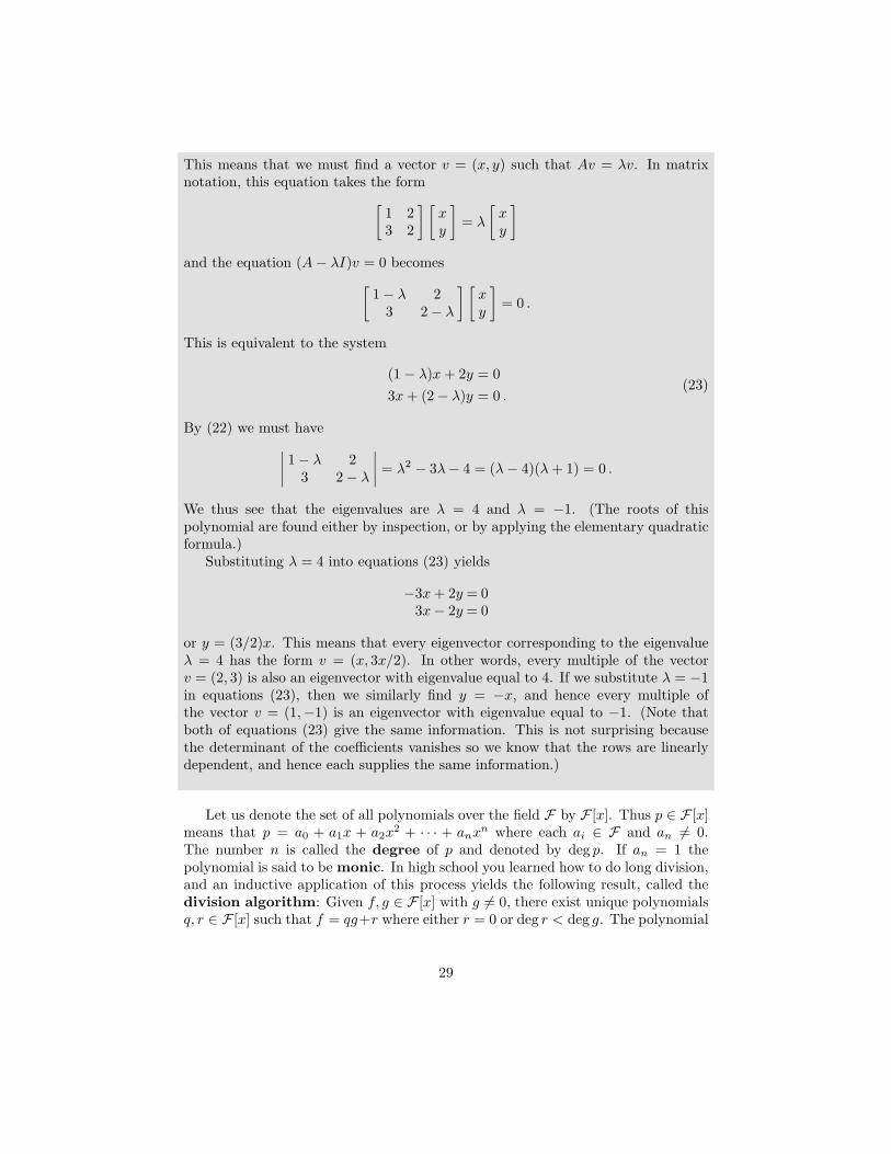
This means that we must find a vector v = (x, y) such that Av = λv. In matrixnotation, this equation takes the form

[1 23 2

] [xy

]= λ

[xy

]

and the equation (A − λI)v = 0 becomes

[1 − λ 2

3 2 − λ

] [xy

]= 0 .

This is equivalent to the system

(1 − λ)x + 2y = 0

3x + (2 − λ)y = 0 .(23)

By (22) we must have

∣∣∣∣1 − λ 2

3 2 − λ

∣∣∣∣ = λ2 − 3λ − 4 = (λ − 4)(λ + 1) = 0 .

We thus see that the eigenvalues are λ = 4 and λ = −1. (The roots of thispolynomial are found either by inspection, or by applying the elementary quadraticformula.)

Substituting λ = 4 into equations (23) yields

−3x + 2y = 03x − 2y = 0

or y = (3/2)x. This means that every eigenvector corresponding to the eigenvalueλ = 4 has the form v = (x, 3x/2). In other words, every multiple of the vectorv = (2, 3) is also an eigenvector with eigenvalue equal to 4. If we substitute λ = −1in equations (23), then we similarly find y = −x, and hence every multiple ofthe vector v = (1,−1) is an eigenvector with eigenvalue equal to −1. (Note thatboth of equations (23) give the same information. This is not surprising becausethe determinant of the coefficients vanishes so we know that the rows are linearlydependent, and hence each supplies the same information.)

Let us denote the set of all polynomials over the field F by F [x]. Thus p ∈ F [x]means that p = a0 + a1x + a2x

2 + · · · + anxn where each ai ∈ F and an 6= 0.The number n is called the degree of p and denoted by deg p. If an = 1 thepolynomial is said to be monic. In high school you learned how to do long division,and an inductive application of this process yields the following result, called thedivision algorithm: Given f, g ∈ F [x] with g 6= 0, there exist unique polynomialsq, r ∈ F [x] such that f = qg+r where either r = 0 or deg r < deg g. The polynomial

29

q is called the quotient and r is called the remainder.If f(x) ∈ F [x], then c ∈ F is said to be a zero or root of f if f(c) = 0. If

f, g ∈ F [x] and g 6= 0, then we say that f is divisible by g (or g divides f) overF if f = qg for some q ∈ F [x]. In other words, f is divisible by g if the remainderin the division of f by g is zero. In this case we also say that g is a factor of f .

Suppose that we divide f by x − c. By the division algorithm we know thatf = (x − c)q + r where either r = 0 or deg r < deg(x − c) = 1. But then eitherr = 0 or deg r = 0 in which case r ∈ F . Either way, substituting x = c we havef(c) = (c − c)q + r = r. Thus the remainder in the division of f by x − c is f(c).This result is called the remainder theorem. As a consequence of this, we seethat x − c will be a factor of f if and only if f(c) = 0, a result called the factor

theorem. If c is such that (x − c)m divides f but no higher power of x− c dividesf , then we say that c is a root of multiplicity m. In counting the number of rootsa polynomial has, we shall always count a root of multiplicity m as m roots. A rootof multiplicity 1 is frequently called a simple root.

The fields R and C are by far the most common fields used by physicists. How-ever, there is an extremely important fundamental difference between them. A fieldF is said to be algebraically closed if every polynomial f ∈ F [x] with deg f > 0has at least one zero (or root) in F . It is a fact (not at all easy to prove) that thecomplex number field C is algebraically closed.

Let F be algebraically closed, and let f ∈ F [x] be of degree n ≥ 1. Since F isalgebraically closed there exists a1 ∈ F such that f(a1) = 0, and hence by the factortheorem, f = (x−a1)q1 where q1 ∈ F [x] and deg q1 = n−1. (This is a consequenceof the general fact that if deg p = m and deg q = n, then deg pq = m + n. Just lookat the largest power of x in the product pq = (a0 + a1x + a2x

2 + · · ·+ amxm)(b0 +b1x + b2x

2 + · · · + bnxn).)Now, by the algebraic closure of F there exists a2 ∈ F such that q1(a2) = 0,

and therefore q1 = (x− a2)q2 where deg q2 = n− 2. It is clear that we can continuethis process a total of n times, finally arriving at

f = c(x − a1)(x − a2) · · · (x − an) = c

n∏

i=1

(x − ai)

where c ∈ F is nonzero. In particular, c = 1 if qn−1 is monic.Observe that while this shows that any polynomial of degree n over an alge-

braically closed field has exactly n roots, it doesn’t require that these roots bedistinct, and in general they are not.

Note also that while the field C is algebraically closed, it is not true that R isalgebraically closed. This should be obvious because any quadratic equation of theform ax2 + bx + c = 0 has solutions given by the quadratic formula

x =−b ±

√b2 − 4ac

2a

and if b2 − 4ac < 0, then there is no solution for x in the real number system.

30

Given a matrix A = (aij) ∈ Mn(F), the trace of A is defined by tr A =∑n

i=1 aii.An important property of the trace is that it is cyclic:

tr AB =

n∑

i=1

(AB)ii =

n∑

i=1

n∑

j=1

aijbji =

n∑

i=1

n∑

j=1

bjiaij =

n∑

j=1

(BA)jj = trBA .

As a consequence of this, we see that the trace is invariant under similarity trans-formations. In other words, if A′ = P−1AP , then tr A′ = tr P−1AP = trAPP−1 =tr A.

Let A ∈ Mn(F) be a matrix representation of T . The matrix xI − A is calledthe characteristic matrix of A, and the expression det(x1 − T ) = 0 is calledthe characteristic (or secular) equation of T . The determinant det(x1 − T ) isfrequently denoted by ∆T (x). Writing out the determinant in a particular basis,we see that det(x1 − T ) is of the form

∆T (x) =

∣∣∣∣∣∣∣∣∣

x − a11 −a12 · · · −a1n

−a21 x − a22 · · · −a2n

......

...−an1 −an2 · · · x − ann

∣∣∣∣∣∣∣∣∣

where A = (aij) is the matrix representation of T in the chosen basis. Since theexpansion of a determinant contains exactly one element from each row and eachcolumn, we see that (and this is a very good exercise for you to show)

det(x1 − T ) = (x − a11)(x − a22) · · · (x − ann)

+ terms containing n − 1 factors of the form x − aii

+ · · · + terms with no factors containing x

= xn − (tr A)xn−1 + terms of lower degree in x + (−1)n detA. (24)

This monic polynomial is called the characteristic polynomial of T .Using Theorem 8 and its corollary, we see that if A′ = P−1AP is similar to A,

then

det(xI − A′) = det(xI − P−1AP ) = det[P−1(xI − A)P ] = det(xI − A) .

We thus see that similar matrices have the same characteristic polynomial (the con-verse of this statement is not true), and hence also the same eigenvalues. Thereforethe eigenvalues (not eigenvectors) of an operator T ∈ L(V ) do not depend on thebasis chosen for V .

Note that since both the determinant and trace are invariant under similaritytransformations, we may as well write trT and detT (rather than tr A and detA)since these are independent of the particular basis chosen.

Since the characteristic polynomial is of degree n in x, it follows from the dis-cussion above that if we are in an algebraically closed field (such as C), then there

31

must exist n roots. In this case the characteristic polynomial may be factored intothe form

det(x1 − T ) = (x − λ1)(x − λ2) · · · (x − λn) (25)

where the eigenvalues λi are not necessarily distinct. Expanding this expression wehave

det(x1 − T ) = xn −(

n∑

i=1

λi

)xn−1 + · · · + (−1)nλ1λ2 · · ·λn.

Comparing this with the above general expression for the characteristic polynomial,we see that

tr T =

n∑

i=1

λi (26a)

and

detT =n∏

i=1

λi. (26b)

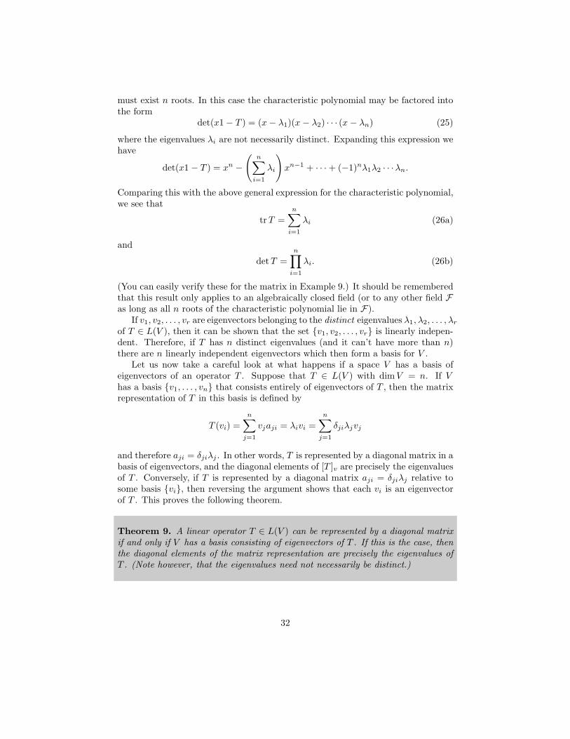
(You can easily verify these for the matrix in Example 9.) It should be rememberedthat this result only applies to an algebraically closed field (or to any other field Fas long as all n roots of the characteristic polynomial lie in F).

If v1, v2, . . . , vr are eigenvectors belonging to the distinct eigenvalues λ1, λ2, . . . , λr

of T ∈ L(V ), then it can be shown that the set {v1, v2, . . . , vr} is linearly indepen-dent. Therefore, if T has n distinct eigenvalues (and it can’t have more than n)there are n linearly independent eigenvectors which then form a basis for V .

Let us now take a careful look at what happens if a space V has a basis ofeigenvectors of an operator T . Suppose that T ∈ L(V ) with dimV = n. If Vhas a basis {v1, . . . , vn} that consists entirely of eigenvectors of T , then the matrixrepresentation of T in this basis is defined by

T (vi) =

n∑

j=1

vjaji = λivi =

n∑

j=1

δjiλjvj

and therefore aji = δjiλj . In other words, T is represented by a diagonal matrix in abasis of eigenvectors, and the diagonal elements of [T ]v are precisely the eigenvaluesof T . Conversely, if T is represented by a diagonal matrix aji = δjiλj relative tosome basis {vi}, then reversing the argument shows that each vi is an eigenvectorof T . This proves the following theorem.

Theorem 9. A linear operator T ∈ L(V ) can be represented by a diagonal matrixif and only if V has a basis consisting of eigenvectors of T . If this is the case, thenthe diagonal elements of the matrix representation are precisely the eigenvalues ofT . (Note however, that the eigenvalues need not necessarily be distinct.)

32

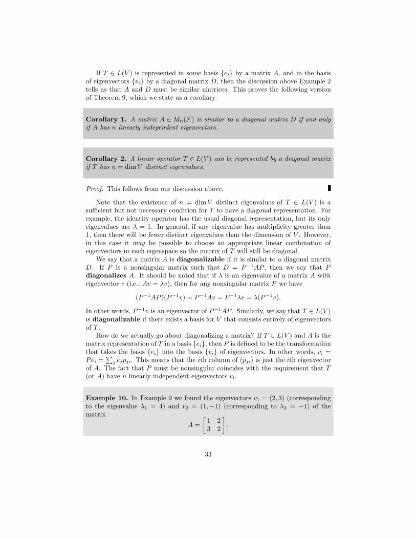
If T ∈ L(V ) is represented in some basis {ei} by a matrix A, and in the basisof eigenvectors {vi} by a diagonal matrix D, then the discussion above Example 2tells us that A and D must be similar matrices. This proves the following versionof Theorem 9, which we state as a corollary.

Corollary 1. A matrix A ∈ Mn(F) is similar to a diagonal matrix D if and onlyif A has n linearly independent eigenvectors.

Corollary 2. A linear operator T ∈ L(V ) can be represented by a diagonal matrixif T has n = dim V distinct eigenvalues.

Proof. This follows from our discussion above.

Note that the existence of n = dimV distinct eigenvalues of T ∈ L(V ) is asufficient but not necessary condition for T to have a diagonal representation. Forexample, the identity operator has the usual diagonal representation, but its onlyeigenvalues are λ = 1. In general, if any eigenvalue has multiplicity greater than1, then there will be fewer distinct eigenvalues than the dimension of V . However,in this case it may be possible to choose an appropriate linear combination ofeigenvectors in each eigenspace so the matrix of T will still be diagonal.

We say that a matrix A is diagonalizable if it is similar to a diagonal matrixD. If P is a nonsingular matrix such that D = P−1AP , then we say that Pdiagonalizes A. It should be noted that if λ is an eigenvalue of a matrix A witheigenvector v (i.e., Av = λv), then for any nonsingular matrix P we have

(P−1AP )(P−1v) = P−1Av = P−1λv = λ(P−1v).

In other words, P−1v is an eigenvector of P−1AP . Similarly, we say that T ∈ L(V )is diagonalizable if there exists a basis for V that consists entirely of eigenvectorsof T .

How do we actually go about diagonalizing a matrix? If T ∈ L(V ) and A is thematrix representation of T in a basis {ei}, then P is defined to be the transformationthat takes the basis {ei} into the basis {vi} of eigenvectors. In other words, vi =Pei =

∑j ejpji. This means that the ith column of (pji) is just the ith eigenvector

of A. The fact that P must be nonsingular coincides with the requirement that T(or A) have n linearly independent eigenvectors vi.

Example 10. In Example 9 we found the eigenvectors v1 = (2, 3) (correspondingto the eigenvalue λ1 = 4) and v2 = (1,−1) (corresponding to λ2 = −1) of thematrix

A =

[1 23 2

].

33

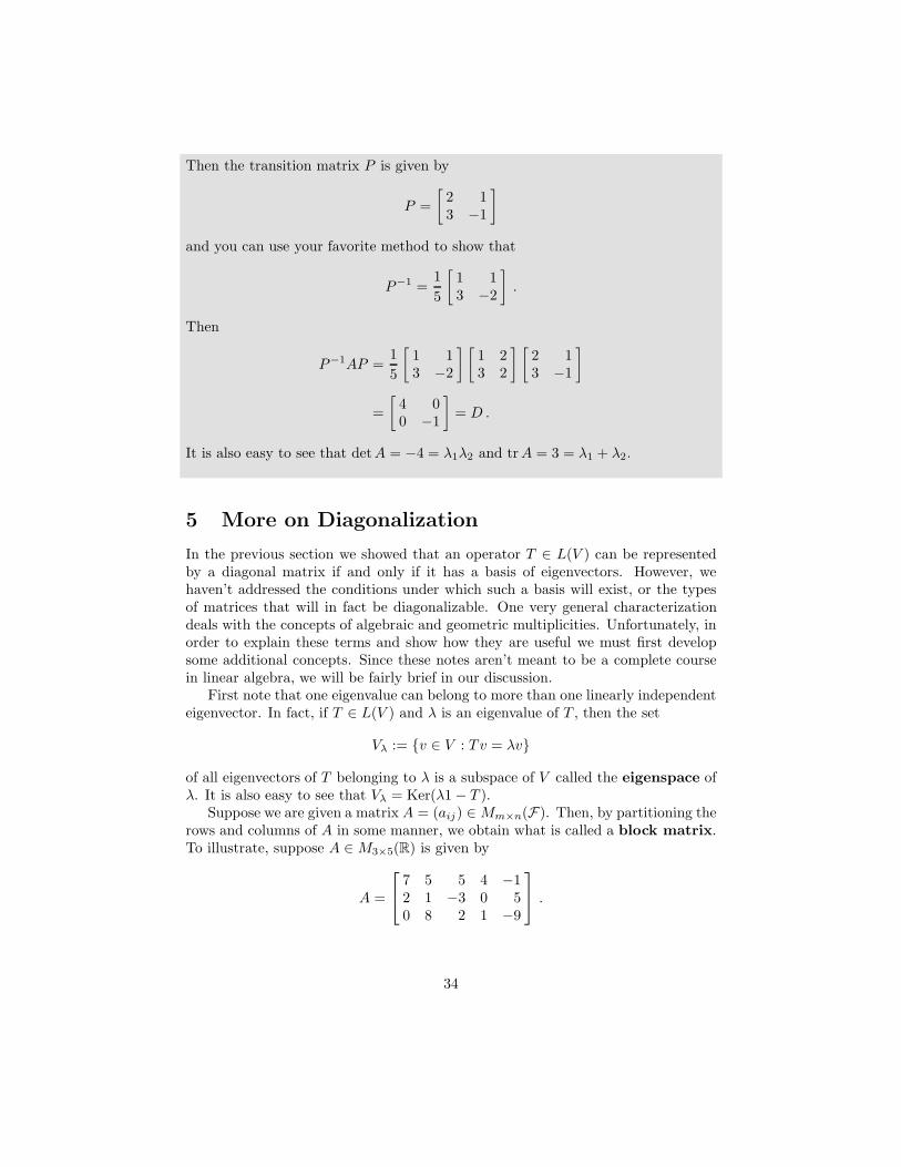
Then the transition matrix P is given by

P =

[2 13 −1

]

and you can use your favorite method to show that

P−1 =1

5

[1 13 −2

].

Then

P−1AP =1

5

[1 13 −2

] [1 23 2

] [2 13 −1

]

=

[4 00 −1

]= D .

It is also easy to see that det A = −4 = λ1λ2 and tr A = 3 = λ1 + λ2.

5 More on Diagonalization

In the previous section we showed that an operator T ∈ L(V ) can be representedby a diagonal matrix if and only if it has a basis of eigenvectors. However, wehaven’t addressed the conditions under which such a basis will exist, or the typesof matrices that will in fact be diagonalizable. One very general characterizationdeals with the concepts of algebraic and geometric multiplicities. Unfortunately, inorder to explain these terms and show how they are useful we must first developsome additional concepts. Since these notes aren’t meant to be a complete coursein linear algebra, we will be fairly brief in our discussion.

First note that one eigenvalue can belong to more than one linearly independenteigenvector. In fact, if T ∈ L(V ) and λ is an eigenvalue of T , then the set

Vλ := {v ∈ V : Tv = λv}

of all eigenvectors of T belonging to λ is a subspace of V called the eigenspace ofλ. It is also easy to see that Vλ = Ker(λ1 − T ).

Suppose we are given a matrix A = (aij) ∈ Mm×n(F). Then, by partitioning therows and columns of A in some manner, we obtain what is called a block matrix.To illustrate, suppose A ∈ M3×5(R) is given by

A =

7 5 5 4 −12 1 −3 0 50 8 2 1 −9

.

34

Then we may partition A into blocks to obtain (for example) the matrix

A =

[A11 A12

A21 A22

]

where

A11 =[7 5 5

]A12 =

[4 −1

]

A21 =

[2 1 −30 8 2

]A22 =

[0 51 −9

].

If A and B are block matrices that are partitioned into the same number ofblocks such that each of the corresponding blocks is of the same size, then it is clearthat (in an obvious notation)

A + B =

A11 + B11 · · · A1n + B1n

......

Am1 + Bm1 · · · Amn + Bmn

.

In addition, if C and D are block matrices such that the number of columns ineach Cij is equal to the number of rows in each Djk, then the product of C and Dis also a block matrix CD where (CD)ik =

∑j CijDjk. Thus block matrices are

multiplied as if each block were just a single element of each matrix in the product.In other words, each (CD)ik is a matrix that is the sum of a product of matrices.The proof of this fact is an exercise in matrix multiplication, and is left to you.

The proof of the next theorem is just a careful analysis of the definition ofdeterminant, and is omitted.

Theorem 10. If A ∈ Mn(F) is a block triangular matrix of the form

A11 A12 A13 · · · A1k

0 A22 A23 · · · A2k

......

......

0 0 0 · · · Akk

where each Aii is a square matrix and the 0’s are zero matrices of appropriate size,then

det A =k∏

i=1

detAii.

35

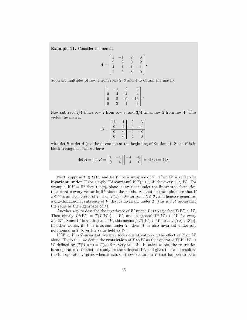
Example 11. Consider the matrix

A =

1 −1 2 32 2 0 24 1 −1 −11 2 3 0

.

Subtract multiples of row 1 from rows 2, 3 and 4 to obtain the matrix

1 −1 2 30 4 −4 −40 5 −9 −130 3 1 −3

.

Now subtract 5/4 times row 2 from row 3, and 3/4 times row 2 from row 4. Thisyields the matrix

B =

1 −1 2 30 4 −4 −40 0 −4 −80 0 4 0

with det B = det A (see the discussion at the beginning of Section 4). Since B is inblock triangular form we have

detA = det B =

∣∣∣∣1 −10 4

∣∣∣∣

∣∣∣∣−4 −8

4 0

∣∣∣∣ = 4(32) = 128.

Next, suppose T ∈ L(V ) and let W be a subspace of V . Then W is said to beinvariant under T (or simply T -invariant) if T (w) ∈ W for every w ∈ W . Forexample, if V = R3 then the xy-plane is invariant under the linear transformationthat rotates every vector in R3 about the z-axis. As another example, note that ifv ∈ V is an eigenvector of T , then T (v) = λv for some λ ∈ F , and hence v generatesa one-dimensional subspace of V that is invariant under T (this is not necessarilythe same as the eigenspace of λ).

Another way to describe the invariance of W under T is to say that T (W ) ⊂ W .Then clearly T 2(W ) = T (T (W )) ⊂ W , and in general T n(W ) ⊂ W for everyn ∈ Z

+. Since W is a subspace of V , this means f(T )(W ) ⊂ W for any f(x) ∈ F [x].In other words, if W is invariant under T , then W is also invariant under anypolynomial in T (over the same field as W ).

If W ⊂ V is T -invariant, we may focus our attention on the effect of T on Walone. To do this, we define the restriction of T to W as that operator T |W : W →W defined by (T |W )(w) = T (w) for every w ∈ W . In other words, the restrictionis an operator T |W that acts only on the subspace W , and gives the same result asthe full operator T gives when it acts on those vectors in V that happen to be in

36

W . We will frequently write TW instead of T |W .Now suppose T ∈ L(V ) and let W ⊂ V be a T -invariant subspace. Furthermore,

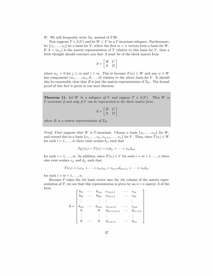
let {v1, . . . , vn} be a basis for V , where the first m < n vectors form a basis for W .If A = (aij) is the matrix representation of T relative to this basis for V , then alittle thought should convince you that A must be of the block matrix form

A =

[B C0 D

]

where aij = 0 for j ≤ m and i > m. This is because T (w) ∈ W and any w ∈ Whas components (w1, . . . , wm, 0, . . . , 0) relative to the above basis for V . It shouldalso be reasonably clear that B is just the matrix representation of TW . The formalproof of this fact is given in our next theorem.

Theorem 11. Let W be a subspace of V and suppose T ∈ L(V ). Then W isT -invariant if and only if T can be represented in the block matrix form

A =

[B C0 D

]

where B is a matrix representation of TW .

Proof. First suppose that W is T -invariant. Choose a basis {v1, . . . , vm} for W ,and extend this to a basis {v1, . . . , vm, vm+1, . . . , vn} for V . Then, since T (vi) ∈ Wfor each i = 1, . . . , m there exist scalars bij such that

TW (vi) = T (vi) = v1b1i + · · · + vmbmi

for each i = 1, . . . , m. In addition, since T (vi) ∈ V for each i = m + 1, . . . , n therealso exist scalars cij and dij such that

T (vi) = v1c1i + · · · + vmcmi + vm+1dm+1,i + · · · + vndni

for each i = m + 1, . . . , n.Because T takes the ith basis vector into the ith column of the matrix repre-

sentation of T , we see that this representation is given by an n×n matrix A of theform

A =

b11 · · · b1m c1 m+1 · · · c1n

b21 · · · b2m c2 m+1 · · · c2n

......

......

bm1 · · · bmm cm m+1 · · · cmn

0 0 dm+1 m+1 · · · dm+1 n

......

......

0 · · · 0 dn m+1 · · · dnn

37

or, in block matrix form as

A =

[B C0 D

]

where B is an m×m matrix that represents TW , C is an m× (n−m) matrix, andD is an (n − m) × (n − m) matrix.

Conversely, if A has the stated form and {v1, . . . , vn} is a basis for V , then thesubspace W of V defined by vectors of the form

w =

m∑

i=1

αivi

where each αi ∈ F will be invariant under T . Indeed, for each i = 1, . . . , m we have

T (vi) =n∑

j=1

vjaji = v1b1i + · · · + vmbmi ∈ W

and hence T (w) =∑m

i=1 αiT (vi) ∈ W .

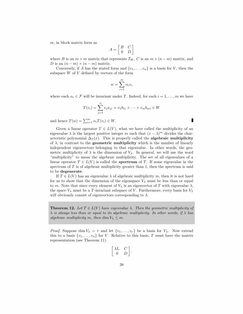
Given a linear operator T ∈ L(V ), what we have called the multiplicity of aneigenvalue λ is the largest positive integer m such that (x − λ)m divides the char-acteristic polynomial ∆T (x). This is properly called the algebraic multiplicity

of λ, in contrast to the geometric multiplicity which is the number of linearlyindependent eigenvectors belonging to that eigenvalue. In other words, the geo-metric multiplicity of λ is the dimension of Vλ. In general, we will use the word“multiplicity” to mean the algebraic multiplicity. The set of all eigenvalues of alinear operator T ∈ L(V ) is called the spectrum of T . If some eigenvalue in thespectrum of T is of algebraic multiplicity greater than 1, then the spectrum is saidto be degenerate.

If T ∈ L(V ) has an eigenvalue λ of algebraic multiplicity m, then it is not hardfor us to show that the dimension of the eigenspace Vλ must be less than or equalto m. Note that since every element of Vλ is an eigenvector of T with eigenvalue λ,the space Vλ must be a T -invariant subspace of V . Furthermore, every basis for Vλ

will obviously consist of eigenvectors corresponding to λ.

Theorem 12. Let T ∈ L(V ) have eigenvalue λ. Then the geometric multiplicity ofλ is always less than or equal to its algebraic multiplicity. In other words, if λ hasalgebraic multiplicity m, then dim Vλ ≤ m.

Proof. Suppose dimVλ = r and let {v1, . . . , vr} be a basis for Vλ. Now extendthis to a basis {v1, . . . , vn} for V . Relative to this basis, T must have the matrixrepresentation (see Theorem 11)

[λIr C0 D

].

38

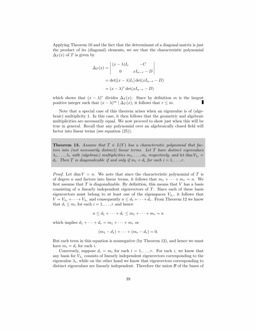
Applying Theorem 10 and the fact that the determinant of a diagonal matrix is justthe product of its (diagonal) elements, we see that the characteristic polynomial∆T (x) of T is given by

∆T (x) =

∣∣∣∣∣(x − λ)Ir −C

0 xIn−r − D

∣∣∣∣∣

= det[(x − λ)Ir ] det(xIn−r − D)

= (x − λ)r det(xIn−r − D)

which shows that (x − λ)r divides ∆T (x). Since by definition m is the largestpositive integer such that (x − λ)m | ∆T (x), it follows that r ≤ m.

Note that a special case of this theorem arises when an eigenvalue is of (alge-braic) multiplicity 1. In this case, it then follows that the geometric and algebraicmultiplicities are necessarily equal. We now proceed to show just when this will betrue in general. Recall that any polynomial over an algebraically closed field willfactor into linear terms (see equation (25)).

Theorem 13. Assume that T ∈ L(V ) has a characteristic polynomial that fac-tors into (not necessarily distinct) linear terms. Let T have distinct eigenvaluesλ1, . . . , λr with (algebraic) multiplicities m1, . . . , mr respectively, and let dimVλi

=di. Then T is diagonalizable if and only if mi = di for each i = 1, . . . , r.

Proof. Let dimV = n. We note that since the characteristic polynomial of T isof degree n and factors into linear terms, it follows that m1 + · · · + mr = n. Wefirst assume that T is diagonalizable. By definition, this means that V has a basisconsisting of n linearly independent eigenvectors of T . Since each of these basiseigenvectors must belong to at least one of the eigenspaces Vλi

, it follows thatV = Vλ1

+ · · ·+Vλrand consequently n ≤ d1 + · · ·+dr. From Theorem 12 we know

that di ≤ mi for each i = 1, . . . , r and hence

n ≤ d1 + · · · + dr ≤ m1 + · · · + mr = n

which implies d1 + · · · + dr = m1 + · · · + mr or

(m1 − d1) + · · · + (mr − dr) = 0.

But each term in this equation is nonnegative (by Theorem 12), and hence we musthave mi = di for each i.

Conversely, suppose di = mi for each i = 1, . . . , r. For each i, we know thatany basis for Vλi

consists of linearly independent eigenvectors corresponding to theeigenvalue λi, while on the other hand we know that eigenvectors corresponding todistinct eigenvalues are linearly independent. Therefore the union B of the bases of

39

{Vλi} forms a linearly independent set of d1 + · · · + dr = m1 + · · · + mr vectors.

But m1 + · · · + mr = n = dimV , and hence B forms a basis for V . Since thisshows that V has a basis of eigenvectors of T , it follows by definition that T mustbe diagonalizable.

Example 12. Consider the operator T ∈ L(R3) defined by

T (x, y, z) = (9x + y, 9y, 7z).

Relative to the standard basis for R3, the matrix representation of T is given by

A =

9 1 00 9 00 0 7

and hence the characteristic polynomial is

∆A(x) = det(A − λI) = (9 − λ)2(7 − λ)

which is a product of linear factors. However,

A − 9I =

0 1 00 0 00 0 −2

which clearly has rank equal to 2, and hence nul(A − 9I) = 3 − 2 = 1 which isnot the same as the algebraic multiplicity of λ = 9 (which is 2). Thus T is notdiagonalizable.

Example 13. Consider the operator on R3 defined by the following matrix:

A =

5 −6 −6−1 4 2

3 −6 −4

.

In order to avoid factoring a cubic polynomial, we compute the characteristic poly-nomial ∆A(x) = det(xI−A) by applying elementary row operations as follows (youshould be able to see exactly what elementary row operations were performed ineach step; see the discussion at the beginning of Section 4).

∣∣∣∣∣∣

x − 5 6 61 x − 4 −2

−3 6 x + 4

∣∣∣∣∣∣=

∣∣∣∣∣∣

x − 2 0 −x + 21 x − 4 −2

−3 6 x + 4

∣∣∣∣∣∣

= (x − 2)

∣∣∣∣∣∣

1 0 −11 x − 4 −2

−3 6 x + 4

∣∣∣∣∣∣

40

= (x − 2)

∣∣∣∣∣∣

1 0 −10 x − 4 −10 6 x + 1

∣∣∣∣∣∣

= (x − 2)

∣∣∣∣x − 4 −1

6 x + 1

∣∣∣∣

= (x − 2)2(x − 1).

We now see that A has eigenvalue λ1 = 1 with (algebraic) multiplicity 1, andeigenvalue λ2 = 2 with (algebraic) multiplicity 2. From Theorem 12 we know thatthe algebraic and geometric multiplicities of λ1 are necessarily the same and equalto 1, so we need only consider λ2. Observing that

A − 2I =

3 −6 −6−1 2 2

3 −6 −6

it is obvious that rank(A− 2I) = 1, and hence nul(A− 2I) = 3− 1 = 2. This showsthat A is indeed diagonalizable.

Let us now construct bases for the eigenspaces Wi = Vλi. This means we seek

vectors v = (x, y, z) ∈ R3 such that (A − λiI)v = 0. This is easily solved by theusual row reduction techniques as follows. For λ1 = 1 we have

A − I =

4 −6 −6

−1 3 23 −6 −5

→

1 0 −1

−1 3 23 −6 −5

→

1 0 −10 3 10 −6 −2

→

1 0 −10 3 10 0 0

which has the solutions x = z and y = −z/3 = −x/3. Therefore W1 is spanned bythe single eigenvector v1 = (3,−1, 3). As to λ2 = 2, we proceed in a similar mannerto obtain

A − 2I =

3 −6 −6−1 2 2

3 −6 −6

→

1 −2 −20 0 00 0 0

which implies that any vector (x, y, z) with x = 2y + 2z will work. For example, wecan let x = 0 and y = 1 to obtain z = −1, and hence one basis vector for W2 isgiven by v2 = (0, 1,−1). If we let x = 1 and y = 0, then we have z = 1/2 so thatanother independent basis vector for W2 is given by v3 = (2, 0, 1).

In terms of these eigenvectors, the transformation matrix P that diagonalizes Ais given by

P =

3 0 2

−1 1 03 −1 1

41

and I leave it to you to verify that AP = PD (i.e., P−1AP = D) where D is thediagonal matrix with diagonal elements d11 = 1 and d22 = d33 = 2.

6 Diagonalizing Normal Matrices

The previous section described some general conditions under which a matrix maybe diagonalized. However, in physics the most useful matrices are either real sym-metric (in the case of Mn(R)), Hermitian (in the case of Mn(C)) or unitary (alsofor Mn(C)). In this section I will show that in fact all of these can always bediagonalized.

One tool that we will find useful is the Gram-Schmidt orthogonalization

process which you have probably seen before. However, just in case, I will give acomplete statement and proof. It will also be useful to note that any orthogonalset of vectors is necessarily linearly independent. To see this, let {v1, . . . , vn} be anorthogonal set, and suppose

∑ni=1 aivi = 0. Taking the inner product with vj we

have

0 =

n∑

i=1

ai〈vj , vi〉 =

n∑

i=1

aiδij = aj .

Since this holds for all j, we have ai = 0 for all i so that {vi} is linearly independentas claimed.

Theorem 14. Let V be a finite-dimensional inner product space. Then there existsan orthonormal set of vectors that forms a basis for V .

Proof. Let dim V = n and let {u1, . . . , un} be a basis for V . We will construct anew basis {w1, . . . , wn} such that 〈wi, wj〉 = δij . To begin, we choose

w1 =u1

‖u1‖

so that

‖w1‖2= 〈w1, w1〉 = 〈u1/ ‖u1‖ , u1/ ‖u1‖〉 = 〈u1, u1〉/ ‖u1‖2

= ‖u1‖2 / ‖u1‖2 = 1

and hence w1 is a unit vector. We now take u2 and subtract off its “projection”along w1. This will leave us with a new vector v2 that is orthogonal to w1. Thus,we define

v2 = u2 − 〈w1, u2〉w1

so that〈w1, v2〉 = 〈w1, u2〉 − 〈w1, u2〉〈w1, w1〉 = 0

42

If we letw2 =

v2

‖v2‖then {w1, w2} is an orthonormal set . (That v2 6= 0 will be shown below.)

We now go to u3 and subtract off its projection along w1 and w2. In otherwords, we define

v3 = u3 − 〈w2, u3〉w2 − 〈w1, u3〉w1

so that 〈w1, v3〉 = 〈w2, v3〉 = 0. Choosing

w3 =v3

‖v3‖

we now have an orthonormal set {w1, w2, w3}.It is now clear that given an orthonormal set {w1, . . . , wk}, we let

vk+1 = uk+1 −k∑

i=1

〈wi, uk+1〉wi

so that vk+1 is orthogonal to w1, . . . , wk, and hence we define

wk+1 =vk+1

‖vk+1‖.

It should now be obvious that we can construct an orthonormal set of n vectorsfrom our original basis of n vectors. To finish the proof, we need only show thatw1, . . . , wn are linearly independent.

To see this, note first that since u1 and u2 are linearly independent, w1 andu2 must also be linearly independent, and hence v2 6= 0 by definition of linearindependence. Thus w2 exists and {w1, w2} is linearly independent (since they areorthogonal). Next, {w1, w2, u3} is linearly independent since w1 and w2 are in thelinear span of u1 and u2. Hence v3 6= 0 so that w3 exists, and again {w1, w2, w3} islinearly independent.

In general then, if {w1, . . . , wk} is linearly independent, it follows that the set{w1, . . . , wk, uk+1} is also independent since {w1, . . . , wk} is in the linear span of{u1, . . . , uk}. Hence vk+1 6= 0 and wk+1 exists. Then {w1, . . . , wk+1} is linearlyindependent. Thus {w1, . . . , wn} forms a basis for V , and 〈wi, wj〉 = δij .

Corollary (Gram-Schmidt process). Let {u1, . . . , un} be a linearly independentset of vectors in an inner product space V . Then there exists a set of orthonormalvectors w1, . . . , wn ∈ V such that the linear span of {u1, . . . , uk} is equal to thelinear span of {w1, . . . , wk} for each k = 1, . . . , n.

Proof. This corollary follows by a careful inspection of the proof of Theorem 14.

43

We emphasize that the Gram-Schmidt algorithm (the “orthogonalization pro-cess” of Theorem 14) as such applies to any inner product space, and is not restrictedto only finite-dimensional spaces.

Example 14. Consider the following basis vectors for R3:

u1 = (3, 0, 4) u2 = (−1, 0, 7) u3 = (2, 9, 11).

Let us apply the Gram-Schmidt process (with the standard inner product on R3)to obtain a new orthonormal basis for R3.

Since ‖u1‖ =√

9 + 16 = 5, we define

w1 = u1/5 = (3/5, 0, 4/5).

Next, using 〈w1, u2〉 = −3/5 + 28/5 = 5 we let

v2 = (−1, 0, 7)− (3, 0, 4) = (−4, 0, 3).

Since ‖v2‖ = 5, we havew2 = (−4/5, 0, 3/5).

Finally, using 〈w1, u3〉 = 10 and 〈w2, u3〉 = 5 we let

v3 = (2, 9, 11)− (−4, 0, 3)− (6, 0, 8) = (0, 9, 0)

and hence, since ‖v3‖ = 9, our third basis vector becomes

w3 = (0, 1, 0).

I leave it to you to show that {w1, w2, w3} does indeed form an orthonormal basisfor R3.

Recall that the transpose of A = (aij) ∈ Mn(C) is the matrix AT = (aij)T =

(aji). Then for any A, B ∈ Mn(C) we have

(AB)Tij = (AB)ji =

n∑

k=1

ajkbki =

n∑

k=1

bTikaT

kj = (BT AT )ij

and therefore (AB)T = BT AT as you should already know.Now suppose we have a matrix A ∈ Mn(C). We define the adjoint (or Hermi-

tian adjoint) of A to be the matrix A† = A∗T . In other words, the adjoint of A isits complex conjugate transpose. From what we just showed, it is easy to see that

(AB)† = B†A†.

If it so happens that A† = A, then A is said to be a Hermitian matrix.

44

If a matrix U ∈ Mn(C) has the property that U † = U−1, then we say U isunitary. Thus a matrix U is unitary if UU † = U †U = I. (I state without proofthat in a finite-dimensional space, it is only necessary to require either UU † = Ior U †U = I. In other words, in finite dimensions (or for any finite group) theexistence of a left (right) inverse implies the existence of a right (left) inverse.However, the full definition is necessary in the case of infinite-dimensional spaces.)We also see that the product of two unitary matrices U and V is unitary since(UV )†UV = V †U †UV = V †IV = V †V = I. If a matrix N ∈ Mn(C) has theproperty that it commutes with its adjoint, i.e., NN † = N †N , then N is said tobe a normal matrix. Note that Hermitian and unitary matrices are automaticallynormal.

Example 15. Consider the matrix A ∈ M2(C) given by

A =1√2

[1 −1i i

].

Then the adjoint of A is given by

A† =1√2

[1 −i

−1 −i

]

and I leave it to you to verify that AA† = A†A = I, and hence show that A isunitary.

A convenient property of the adjoint is this. If A ∈ Mn(C) and x, y ∈ Cn, thenAx ∈ Cn also, so we may use the standard inner product on Cn to write (usingA† = A∗T )

〈Ax, y〉 =

n∑

i=1

(Ax)∗i yi =

n∑

i=1

a∗ijx

∗jyi =

n∑

i=1

x∗ja

†jiyi

= 〈x, A†y〉. (27)

In the particular case of a unitary matrix, we see that

〈Ux, Uy〉 = 〈x, U †Uy〉 = 〈x, y〉

so that unitary transformations also preserve the angle between two vectors (andhence maintains orthogonality as well). Choosing y = x we also see that

‖Ux‖2= 〈Ux, Ux〉 = 〈x, U †Ux〉 = 〈x, Ix〉 = 〈x, x〉 = ‖x‖2

so that unitary transformations preserve lengths of vectors, i.e., they are really justrotations in Cn.

45

It is well worth pointing out that in the case of a real matrix A ∈ Mn(R), insteadof the adjoint A† we have the transpose AT and equation (27) becomes

〈Ax, y〉 = 〈x, AT y〉

or equivalently〈AT x, y〉 = 〈x, Ay〉. (28)

We will use this below when we prove that a real symmetric matrix has all realeigenvalues.

Note that since U ∈ Mn(C), the rows Ui and columns U i of U are just vectorsin Cn. This means we can take their inner product relative to the standard innerproduct on Cn. Writing out the relation UU † = I in terms of components, we have

(UU †)ij =

n∑

k=1

uiku†kj =

n∑

k=1

uiku∗jk =

n∑

k=1

u∗jkuik = 〈Uj , Ui〉 = δij

and from U †U = I we see that

(U †U)ij =

n∑

k=1

u†ikukj =

n∑

k=1

u∗kiukj = 〈U i, U j〉 = δij .

In other words, a matrix is unitary if and only if its rows (or columns) each forman orthonormal set. Note we have shown that if the rows (columns) of U ∈ Mn(C)form an orthonormal set, then so do the columns (rows), and either of these is asufficient condition for U to be unitary. For example, you can easily verify that thematrix A in Example 15 satisfies these conditions.

It is also worth pointing out that Hermitian and unitary matrices have importantanalogues over the real number system. If A ∈ Mn(R) is Hermitian, then A = A† =AT , and we say A is symmetric. If U ∈ Mn(R) is unitary, then U−1 = U † = UT ,and we say U is orthogonal. Repeating the above calculations over R, it is easyto see that a real matrix is orthogonal if and only if its rows (or columns) form anorthonormal set.

Let us summarize what we have shown so far in this section.

Theorem 15. The following conditions on a matrix U ∈ Mn(C) are equivalent:(i) U is unitary.(ii) The rows Ui of U form an orthonormal set.(iii) The columns U i of U form an orthonormal set.

Note that the equivalence of (ii) and (iii) in this theorem means that the rowsof U form an orthonormal set if and only if the columns of U form an orthonormalset. But the rows of U are just the columns of UT , and hence U is unitary if andonly if UT is unitary.

46

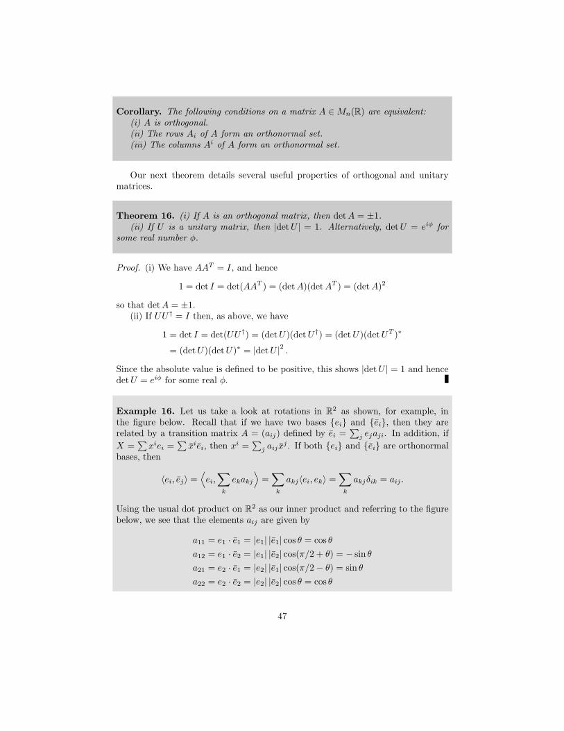
Corollary. The following conditions on a matrix A ∈ Mn(R) are equivalent:(i) A is orthogonal.(ii) The rows Ai of A form an orthonormal set.(iii) The columns Ai of A form an orthonormal set.

Our next theorem details several useful properties of orthogonal and unitarymatrices.

Theorem 16. (i) If A is an orthogonal matrix, then detA = ±1.(ii) If U is a unitary matrix, then |detU | = 1. Alternatively, detU = eiφ for

some real number φ.

Proof. (i) We have AAT = I, and hence

1 = det I = det(AAT ) = (det A)(det AT ) = (det A)2

so that detA = ±1.(ii) If UU † = I then, as above, we have

1 = det I = det(UU †) = (detU)(det U †) = (det U)(detUT )∗

= (detU)(detU)∗ = |det U |2 .

Since the absolute value is defined to be positive, this shows |detU | = 1 and hencedetU = eiφ for some real φ.

Example 16. Let us take a look at rotations in R2 as shown, for example, inthe figure below. Recall that if we have two bases {ei} and {ei}, then they arerelated by a transition matrix A = (aij) defined by ei =

∑j ejaji. In addition, if

X =∑

xiei =∑

xiei, then xi =∑

j aij xj . If both {ei} and {ei} are orthonormal

bases, then

〈ei, ej〉 =⟨ei,∑

k

ekakj

⟩=∑

k

akj〈ei, ek〉 =∑

k

akjδik = aij .

Using the usual dot product on R2 as our inner product and referring to the figurebelow, we see that the elements aij are given by

a11 = e1 · e1 = |e1| |e1| cos θ = cos θ

a12 = e1 · e2 = |e1| |e2| cos(π/2 + θ) = − sin θ

a21 = e2 · e1 = |e2| |e1| cos(π/2 − θ) = sin θ

a22 = e2 · e2 = |e2| |e2| cos θ = cos θ

47

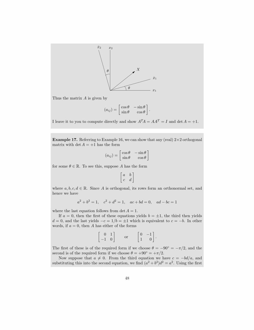
x1

x2

x1

x2

θ

θ X

Thus the matrix A is given by

(aij) =

[cos θ − sin θsin θ cos θ

].

I leave it to you to compute directly and show ATA = AAT = I and detA = +1.

Example 17. Referring to Example 16, we can show that any (real) 2×2 orthogonalmatrix with detA = +1 has the form

(aij) =

[cos θ − sin θsin θ cos θ

]

for some θ ∈ R. To see this, suppose A has the form

[a bc d

]

where a, b, c, d ∈ R. Since A is orthogonal, its rows form an orthonormal set, andhence we have

a2 + b2 = 1, c2 + d2 = 1, ac + bd = 0, ad − bc = 1

where the last equation follows from detA = 1.If a = 0, then the first of these equations yields b = ±1, the third then yields

d = 0, and the last yields −c = 1/b = ±1 which is equivalent to c = −b. In otherwords, if a = 0, then A has either of the forms

[0 1

−1 0

]or

[0 −11 0

].

The first of these is of the required form if we choose θ = −90◦ = −π/2, and thesecond is of the required form if we choose θ = +90◦ = +π/2.

Now suppose that a 6= 0. From the third equation we have c = −bd/a, andsubstituting this into the second equation, we find (a2 + b2)d2 = a2. Using the first

48

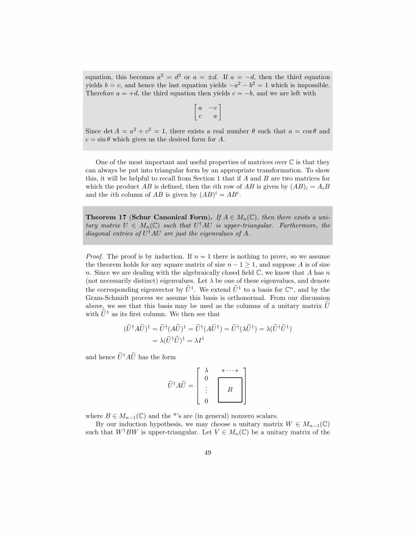
equation, this becomes a2 = d2 or a = ±d. If a = −d, then the third equationyields b = c, and hence the last equation yields −a2 − b2 = 1 which is impossible.Therefore a = +d, the third equation then yields c = −b, and we are left with

[a −cc a

]

Since detA = a2 + c2 = 1, there exists a real number θ such that a = cos θ andc = sin θ which gives us the desired form for A.

One of the most important and useful properties of matrices over C is that theycan always be put into triangular form by an appropriate transformation. To showthis, it will be helpful to recall from Section 1 that if A and B are two matrices forwhich the product AB is defined, then the ith row of AB is given by (AB)i = AiBand the ith column of AB is given by (AB)i = ABi.

Theorem 17 (Schur Canonical Form). If A ∈ Mn(C), then there exists a uni-tary matrix U ∈ Mn(C) such that U †AU is upper-triangular. Furthermore, thediagonal entries of U †AU are just the eigenvalues of A.

Proof. The proof is by induction. If n = 1 there is nothing to prove, so we assumethe theorem holds for any square matrix of size n− 1 ≥ 1, and suppose A is of sizen. Since we are dealing with the algebraically closed field C, we know that A has n(not necessarily distinct) eigenvalues. Let λ be one of these eigenvalues, and denote

the corresponding eigenvector by U1. We extend U1 to a basis for Cn, and by theGram-Schmidt process we assume this basis is orthonormal. From our discussionabove, we see that this basis may be used as the columns of a unitary matrix Uwith U1 as its first column. We then see that

(U †AU)1 = U †(AU )1 = U †(AU1) = U †(λU1) = λ(U †U1)

= λ(U †U)1 = λI1

and hence U †AU has the form

U †AU =

λ ∗ · · · ∗0...

0

B

where B ∈ Mn−1(C) and the *’s are (in general) nonzero scalars.By our induction hypothesis, we may choose a unitary matrix W ∈ Mn−1(C)

such that W †BW is upper-triangular. Let V ∈ Mn(C) be a unitary matrix of the

49

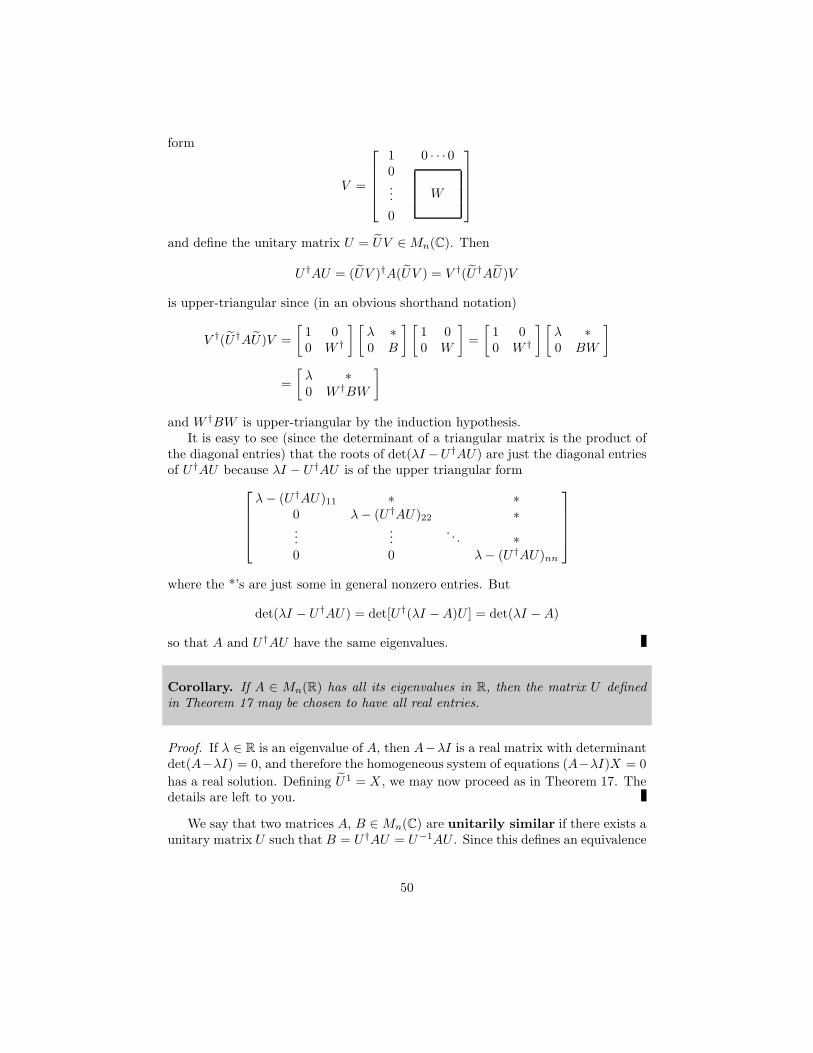
form

V =

1 0 · · · 00...

0

W

and define the unitary matrix U = UV ∈ Mn(C). Then

U †AU = (UV )†A(UV ) = V †(U †AU)V

is upper-triangular since (in an obvious shorthand notation)

V †(U †AU)V =

[1 00 W †

] [λ ∗0 B

] [1 00 W

]=

[1 00 W †

] [λ ∗0 BW

]

=

[λ ∗0 W †BW

]

and W †BW is upper-triangular by the induction hypothesis.It is easy to see (since the determinant of a triangular matrix is the product of

the diagonal entries) that the roots of det(λI −U †AU) are just the diagonal entriesof U †AU because λI − U †AU is of the upper triangular form

λ − (U †AU)11 ∗ ∗0 λ − (U †AU)22 ∗...

.... . . ∗

0 0 λ − (U †AU)nn

where the *’s are just some in general nonzero entries. But

det(λI − U †AU) = det[U †(λI − A)U ] = det(λI − A)

so that A and U †AU have the same eigenvalues.

Corollary. If A ∈ Mn(R) has all its eigenvalues in R, then the matrix U definedin Theorem 17 may be chosen to have all real entries.

Proof. If λ ∈ R is an eigenvalue of A, then A−λI is a real matrix with determinantdet(A−λI) = 0, and therefore the homogeneous system of equations (A−λI)X = 0

has a real solution. Defining U1 = X , we may now proceed as in Theorem 17. Thedetails are left to you.

We say that two matrices A, B ∈ Mn(C) are unitarily similar if there exists aunitary matrix U such that B = U †AU = U−1AU . Since this defines an equivalence

50

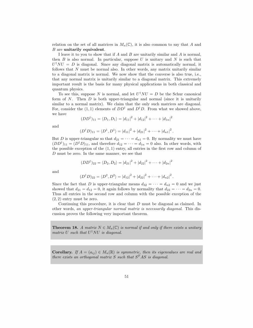
relation on the set of all matrices in Mn(C), it is also common to say that A andB are unitarily equivalent.

I leave it to you to show that if A and B are unitarily similar and A is normal,then B is also normal. In particular, suppose U is unitary and N is such thatU †NU = D is diagonal. Since any diagonal matrix is automatically normal, itfollows that N must be normal also. In other words, any matrix unitarily similarto a diagonal matrix is normal. We now show that the converse is also true, i.e.,that any normal matrix is unitarily similar to a diagonal matrix. This extremelyimportant result is the basis for many physical applications in both classical andquantum physics.

To see this, suppose N is normal, and let U †NU = D be the Schur canonicalform of N . Then D is both upper-triangular and normal (since it is unitarilysimilar to a normal matrix). We claim that the only such matrices are diagonal.For, consider the (1, 1) elements of DD† and D†D. From what we showed above,we have

(DD†)11 = 〈D1, D1〉 = |d11|2 + |d12|2 + · · · + |d1n|2

and(D†D)11 = 〈D1, D1〉 = |d11|2 + |d21|2 + · · · + |dn1|2 .

But D is upper-triangular so that d21 = · · · = dn1 = 0. By normality we must have(DD†)11 = (D†D)11, and therefore d12 = · · · = d1n = 0 also. In other words, withthe possible exception of the (1, 1) entry, all entries in the first row and column ofD must be zero. In the same manner, we see that

(DD†)22 = 〈D2, D2〉 = |d21|2 + |d22|2 + · · · + |d2n|2

and(D†D)22 = 〈D2, D2〉 = |d12|2 + |d22|2 + · · · + |dn2|2 .

Since the fact that D is upper-triangular means d32 = · · · = dn2 = 0 and we justshowed that d21 = d12 = 0, it again follows by normality that d23 = · · · = d2n = 0.Thus all entries in the second row and column with the possible exception of the(2, 2) entry must be zero.

Continuing this procedure, it is clear that D must be diagonal as claimed. Inother words, an upper-triangular normal matrix is necessarily diagonal. This dis-cussion proves the following very important theorem.

Theorem 18. A matrix N ∈ Mn(C) is normal if and only if there exists a unitarymatrix U such that U †NU is diagonal.

Corollary. If A = (aij) ∈ Mn(R) is symmetric, then its eigenvalues are real andthere exists an orthogonal matrix S such that ST AS is diagonal.

51

Proof. If the eigenvalues are real, then the rest of this corollary follows from thecorollary to Theorem 17 and the real analogue of the proof of Theorem 18.

Now suppose A = AT so that aij = aji. If λ is an eigenvalue of A, then thereexists a (nonzero and not necessarily real) vector x ∈ Cn such that Ax = λx andhence

〈x, Ax〉 = λ〈x, x〉 = λ ‖x‖2.

On the other hand, using equation (28) we see that

〈x, Ax〉 = 〈AT x, x〉 = 〈x, AT x〉∗ = 〈x, Ax〉∗ = λ∗〈x, x〉∗ = λ∗ ‖x‖2.

Subtracting these last two equations yields (λ − λ∗) ‖x‖2= 0 and hence λ = λ∗

since ‖x‖ 6= 0 by definition.

Let me make some observations. Note that any basis relative to which a normalmatrix N is diagonal is by definition a basis of eigenvectors. The unitary transitionmatrix U that diagonalizes N has columns that are precisely these eigenvectors,and since the columns of a unitary matrix are orthonormal, it follows that theeigenvector basis is in fact orthonormal. Of course, the analogous result holds for areal symmetric matrix also.

52

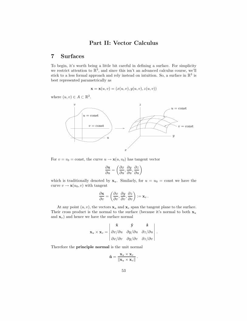
Part II: Vector Calculus

7 Surfaces

To begin, it’s worth being a little bit careful in defining a surface. For simplicitywe restrict attention to R3, and since this isn’t an advanced calculus course, we’llstick to a less formal approach and rely instead on intuition. So, a surface in R3 isbest represented parametrically as

x = x(u, v) = (x(u, v), y(u, v), z(u, v))

where (u, v) ∈ A ⊂ R2.

u

v

x

y

zu = const

u = const

v = constv = const

For v = v0 = const, the curve u → x(u, v0) has tangent vector

∂x

∂u=

(∂x

∂u,∂y

∂u,∂z

∂u

)

which is traditionally denoted by xu. Similarly, for u = u0 = const we have thecurve v → x(u0, v) with tangent

∂x

∂v=

(∂x

∂v,∂y

∂v,∂z

∂v

):= xv .

At any point (u, v), the vectors xu and xv span the tangent plane to the surface.Their cross product is the normal to the surface (because it’s normal to both xu

and xv) and hence we have the surface normal

xu × xv =

∣∣∣∣∣∣∣

x y z

∂x/∂u ∂y/∂u ∂z/∂u

∂x/∂v ∂y/∂v ∂z/∂v

∣∣∣∣∣∣∣.

Therefore the principle normal is the unit normal

n =xu × xv

‖xu × xv‖.

53

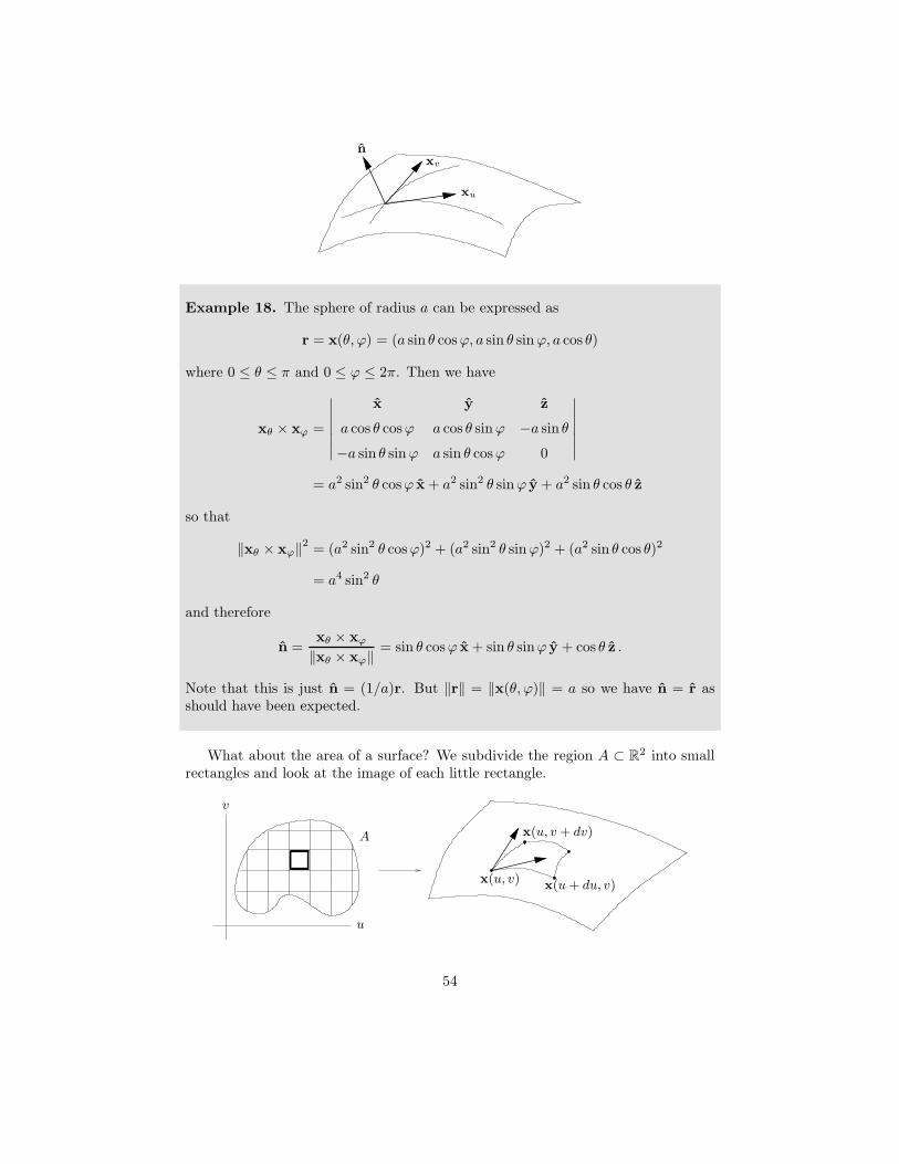
xu

xv

n

Example 18. The sphere of radius a can be expressed as

r = x(θ, ϕ) = (a sin θ cosϕ, a sin θ sin ϕ, a cos θ)

where 0 ≤ θ ≤ π and 0 ≤ ϕ ≤ 2π. Then we have

xθ × xϕ =

∣∣∣∣∣∣∣

x y z

a cos θ cosϕ a cos θ sin ϕ −a sin θ

−a sin θ sin ϕ a sin θ cosϕ 0

∣∣∣∣∣∣∣

= a2 sin2 θ cosϕ x + a2 sin2 θ sin ϕ y + a2 sin θ cos θ z

so that

‖xθ × xϕ‖2= (a2 sin2 θ cosϕ)2 + (a2 sin2 θ sin ϕ)2 + (a2 sin θ cos θ)2

= a4 sin2 θ

and therefore

n =xθ × xϕ

‖xθ × xϕ‖= sin θ cosϕ x + sin θ sinϕ y + cos θ z .

Note that this is just n = (1/a)r. But ‖r‖ = ‖x(θ, ϕ)‖ = a so we have n = r asshould have been expected.

What about the area of a surface? We subdivide the region A ⊂ R2 into smallrectangles and look at the image of each little rectangle.

A

u

v

x(u, v)x(u + du, v)

x(u, v + dv)

54

For the infinitesimal rectangle on the surface we have the distance between pointsgiven by

x(u + du, v) − x(u, v) ≈ ∂x

∂udu = xu du

x(u, v + dv) − x(u, v) ≈ ∂x

∂vdv = xv dv

so the element of area is

dS = ‖xudu × xvdv‖ = ‖xu × xv‖ du dv

and hence that total area of the surface is given by

S =

∫

A

‖xu × xv‖ du dv .

It also follows that the integral of a function f(x, y, z) over the surface is given by

∫

A

f(x, y, z) dS =

∫

A

f(x(u, v), y(u, v), z(u, v)) ‖xu × xv‖ du dv .

8 Gradients

Now let us consider the gradient of a function f(x, y, z). We know that the differ-ential of the function is given by

df =∂f

∂xdx +

∂f

∂ydy +

∂f

∂zdz .

Since dx = dx x + dy y + dz z, we may define the vector

∇f =∂f

∂xx +

∂f

∂yy +

∂f

∂zz

so thatdf = ∇f · dx .

The vector operator ∇ is called the gradient vector:

∇ =

(∂

∂x,

∂

∂y,

∂

∂z

)= x

∂

∂x+ y

∂

∂y+ z

∂

∂z.

To understand what this represents physically, suppose that the displacementdx is in the direction of constant f , i.e., dx is tangent to the surface f = const.Then clearly df = 0 in that direction so that df = ∇f · dx = 0. But this meansthat ∇f⊥dx; in other words, the gradient is orthogonal to the surface. And sincedf = ∇f · dx = ‖∇f‖ ‖dx‖ cos θ, this shows that df will be largest when cos θ = 1,i.e., when dx points along ∇f .

55

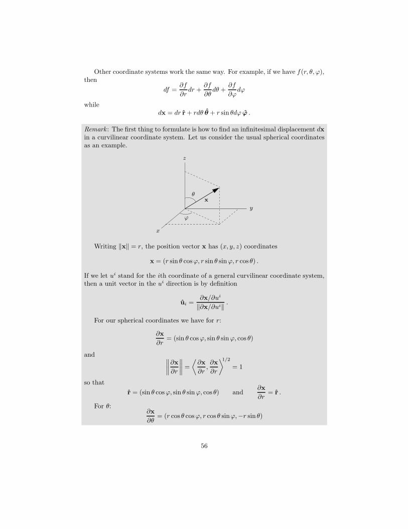
Other coordinate systems work the same way. For example, if we have f(r, θ, ϕ),then

df =∂f

∂rdr +

∂f

∂θdθ +

∂f

∂ϕdϕ

whiledx = dr r + rdθ θ + r sin θdϕ ϕ .

Remark : The first thing to formulate is how to find an infinitesimal displacement dxin a curvilinear coordinate system. Let us consider the usual spherical coordinatesas an example.

x

y

z

θ

ϕ

x

Writing ‖x‖ = r, the position vector x has (x, y, z) coordinates

x = (r sin θ cosϕ, r sin θ sin ϕ, r cos θ) .

If we let ui stand for the ith coordinate of a general curvilinear coordinate system,then a unit vector in the ui direction is by definition

ui =∂x/∂ui

‖∂x/∂ui‖ .

For our spherical coordinates we have for r:

∂x

∂r= (sin θ cosϕ, sin θ sin ϕ, cos θ)

and ∥∥∥∥∂x

∂r

∥∥∥∥ =

⟨∂x

∂r,∂x

∂r

⟩1/2

= 1

so that

r = (sin θ cosϕ, sin θ sin ϕ, cos θ) and∂x

∂r= r .

For θ:∂x

∂θ= (r cos θ cosϕ, r cos θ sinϕ,−r sin θ)

56

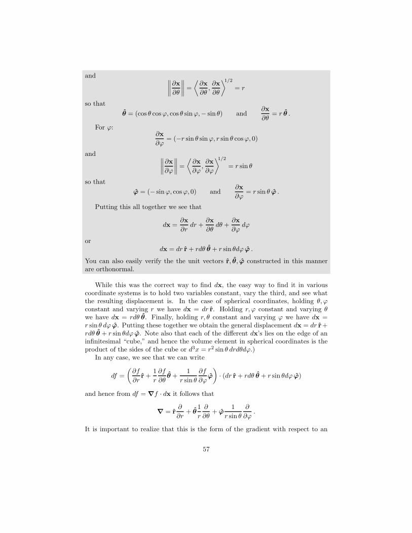
and ∥∥∥∥∂x

∂θ

∥∥∥∥ =

⟨∂x

∂θ,∂x

∂θ

⟩1/2

= r

so that

θ = (cos θ cosϕ, cos θ sin ϕ,− sin θ) and∂x

∂θ= r θ .

For ϕ:∂x

∂ϕ= (−r sin θ sin ϕ, r sin θ cosϕ, 0)

and ∥∥∥∥∂x

∂ϕ

∥∥∥∥ =

⟨∂x

∂ϕ,∂x

∂ϕ

⟩1/2

= r sin θ

so that

ϕ = (− sin ϕ, cosϕ, 0) and∂x

∂ϕ= r sin θ ϕ .

Putting this all together we see that

dx =∂x

∂rdr +

∂x

∂θdθ +

∂x

∂ϕdϕ

ordx = dr r + rdθ θ + r sin θdϕ ϕ .

You can also easily verify the the unit vectors r, θ, ϕ constructed in this mannerare orthonormal.

While this was the correct way to find dx, the easy way to find it in variouscoordinate systems is to hold two variables constant, vary the third, and see whatthe resulting displacement is. In the case of spherical coordinates, holding θ, ϕconstant and varying r we have dx = dr r. Holding r, ϕ constant and varying θwe have dx = rdθ θ. Finally, holding r, θ constant and varying ϕ we have dx =r sin θ dϕ ϕ. Putting these together we obtain the general displacement dx = dr r+rdθ θ + r sin θdϕ ϕ. Note also that each of the different dx’s lies on the edge of aninfinitesimal “cube,” and hence the volume element in spherical coordinates is theproduct of the sides of the cube or d3x = r2 sin θ drdθdϕ.)

In any case, we see that we can write

df =

(∂f

∂rr +

1

r

∂f

∂θθ +

1

r sin θ

∂f

∂ϕϕ

)· (dr r + rdθ θ + r sin θdϕ ϕ)

and hence from df = ∇f · dx it follows that

∇ = r∂

∂r+ θ

1

r

∂

∂θ+ ϕ

1

r sin θ

∂

∂ϕ.

It is important to realize that this is the form of the gradient with respect to an

57

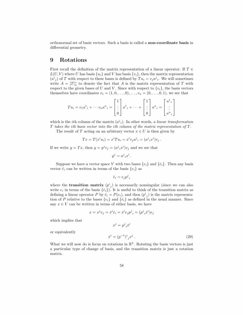
orthonormal set of basis vectors. Such a basis is called a non-coordinate basis indifferential geometry.

9 Rotations

First recall the definition of the matrix representation of a linear operator: If T ∈L(U, V ) where U has basis {ui} and V has basis {vi}, then the matrix representation(ai

j) of T with respect to these bases is defined by Tui = vjaji. We will sometimes

write A = [T ]vu to denote the fact that A is the matrix representation of T withrespect to the given bases of U and V . Since with respect to {vi}, the basis vectorsthemselves have coordinates v1 = (1, 0, . . . , 0), . . . , vn = (0, . . . , 0, 1), we see that

Tui = v1a1i + · · · vnan

i =

1...0

a1

i + · · · +

1...0

an

i =

a1i

...an

i

which is the ith column of the matrix (aji). In other words, a linear transformation

T takes the ith basis vector into the ith column of the matrix representation of T .The result of T acting on an arbitrary vector x ∈ U is then given by

Tx = T (xiui) = xiTui = xivjaji = (aj

ixi)vj .

If we write y = Tx, then y = yjvj = (ajix

i)vj and we see that

yj = ajix

i .

Suppose we have a vector space V with two bases {ei} and {ei}. Then any basisvector ei can be written in terms of the basis {ei} as

ei = ejpji

where the transition matrix (pij) is necessarily nonsingular (since we can also

write ei in terms of the basis {ei}). It is useful to think of the transition matrix asdefining a linear operator P by ei = P (ei), and then (pi

j) is the matrix representa-tion of P relative to the bases {ei} and {ei} as defined in the usual manner. Sinceany x ∈ V can be written in terms of either basis, we have

x = xjej = xiei = xiejpji = (pj

ixi)ej

which implies thatxj = pj

ixi

or equivalentlyxi = (p−1)i

jxj . (29)

What we will now do is focus on rotations in R2. Rotating the basis vectors is justa particular type of change of basis, and the transition matrix is just a rotationmatrix.

58

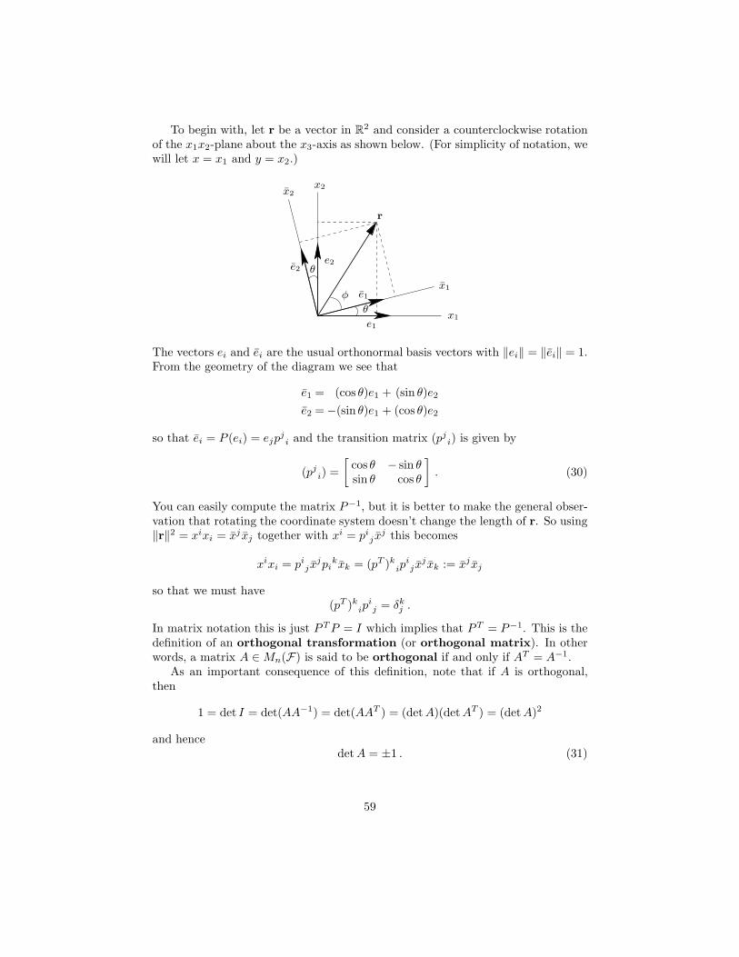
To begin with, let r be a vector in R2 and consider a counterclockwise rotationof the x1x2-plane about the x3-axis as shown below. (For simplicity of notation, wewill let x = x1 and y = x2.)

θ

θ

φ

x1

x2

x1

x2

r

e1

e2

e1

e2

The vectors ei and ei are the usual orthonormal basis vectors with ‖ei‖ = ‖ei‖ = 1.From the geometry of the diagram we see that

e1 = (cos θ)e1 + (sin θ)e2

e2 = −(sin θ)e1 + (cos θ)e2

so that ei = P (ei) = ejpji and the transition matrix (pj

i) is given by

(pji) =

[cos θ − sin θsin θ cos θ

]. (30)

You can easily compute the matrix P−1, but it is better to make the general obser-vation that rotating the coordinate system doesn’t change the length of r. So using‖r‖2 = xixi = xj xj together with xi = pi

j xj this becomes

xixi = pij x

jpikxk = (pT )k

ipij x

j xk := xj xj

so that we must have(pT )k

ipij = δk

j .

In matrix notation this is just PT P = I which implies that PT = P−1. This is thedefinition of an orthogonal transformation (or orthogonal matrix). In otherwords, a matrix A ∈ Mn(F) is said to be orthogonal if and only if AT = A−1.

As an important consequence of this definition, note that if A is orthogonal,then

1 = det I = det(AA−1) = det(AAT ) = (det A)(det AT ) = (det A)2

and hencedet A = ±1 . (31)

59

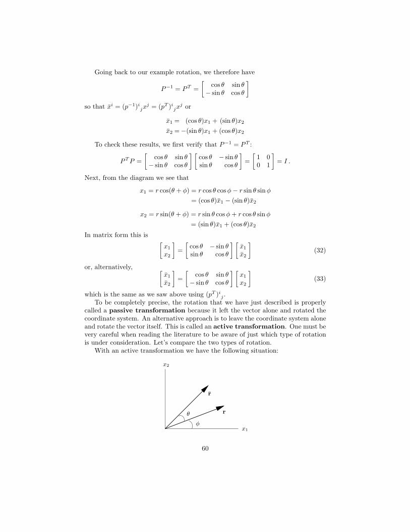
Going back to our example rotation, we therefore have

P−1 = PT =

[cos θ sin θ

− sin θ cos θ

]

so that xi = (p−1)ijx

j = (pT )ijx

j or

x1 = (cos θ)x1 + (sin θ)x2

x2 = −(sin θ)x1 + (cos θ)x2

To check these results, we first verify that P−1 = PT :

PT P =

[cos θ sin θ

− sin θ cos θ

] [cos θ − sin θsin θ cos θ

]=

[1 00 1

]= I .

Next, from the diagram we see that

x1 = r cos(θ + φ) = r cos θ cosφ − r sin θ sin φ

= (cos θ)x1 − (sin θ)x2

x2 = r sin(θ + φ) = r sin θ cosφ + r cos θ sinφ

= (sin θ)x1 + (cos θ)x2

In matrix form this is[

x1

x2

]=

[cos θ − sin θsin θ cos θ

] [x1

x2

](32)

or, alternatively, [x1

x2

]=

[cos θ sin θ

− sin θ cos θ

] [x1

x2

](33)

which is the same as we saw above using (pT )ij .

To be completely precise, the rotation that we have just described is properlycalled a passive transformation because it left the vector alone and rotated thecoordinate system. An alternative approach is to leave the coordinate system aloneand rotate the vector itself. This is called an active transformation. One must bevery careful when reading the literature to be aware of just which type of rotationis under consideration. Let’s compare the two types of rotation.

With an active transformation we have the following situation:

x1

x2

r

r

θ

φ

60

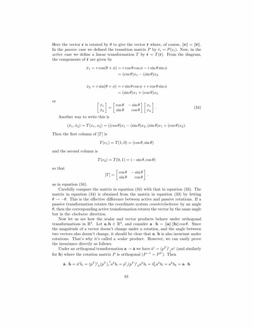
Here the vector r is rotated by θ to give the vector r where, of course, ‖r‖ = ‖r‖.In the passive case we defined the transition matrix P by ei = P (ei). Now, in theactive case we define a linear transformation T by r = T (r). From the diagram,the components of r are given by

x1 = r cos(θ + φ) = r cos θ cosφ − r sin θ sin φ

= (cos θ)x1 − (sin θ)x2

x2 = r sin(θ + φ) = r sin θ cosφ + r cos θ sinφ

= (sin θ)x1 + (cos θ)x2

or [x1

x2

]=

[cos θ − sin θsin θ cos θ

] [x1

x2

]. (34)

Another way to write this is

(x1, x2) = T (x1, x2) = ((cos θ)x1 − (sin θ)x2, (sin θ)x1 + (cos θ)x2).

Then the first column of [T ] is

T (e1) = T (1, 0) = (cos θ, sin θ)

and the second column is

T (e2) = T (0, 1) = (− sin θ, cos θ)

so that

[T ] =

[cos θ − sin θsin θ cos θ

].

as in equation (34).Carefully compare the matrix in equation (34) with that in equation (33). The

matrix in equation (34) is obtained from the matrix in equation (33) by lettingθ → −θ. This is the effective difference between active and passive rotations. If apassive transformation rotates the coordinate system counterclockwise by an angleθ, then the corresponding active transformation rotates the vector by the same anglebut in the clockwise direction.

Now let us see how the scalar and vector products behave under orthogonaltransformations in R3. Let a,b ∈ R3, and consider a · b = ‖a‖ ‖b‖ cos θ. Sincethe magnitude of a vector doesn’t change under a rotation, and the angle betweentwo vectors also doesn’t change, it should be clear that a · b is also invariant underrotations. That’s why it’s called a scalar product. However, we can easily provethe invariance directly as follows.

Under an orthogonal transformation a → a we have ai = (pT )ija

j (and similarly

for b) where the rotation matrix P is orthogonal (P−1 = PT ). Then

a · b = aibi = (pT )ik(pT )i

lakbl = pl

i(pT )i

kakbl = δlkakbl = akbk = a · b

61

so that the scalar product is indeed invariant under orthogonal transformations.However, what can we say about the cross product? Since the definition of

a × b depends on the right-hand rule, it is reasonable to suspect that there willbe some kind of dependence on the particular orthogonal transformation (since weknow that the determinant of an orthogonal transformation can be either +1 or−1). Proceeding as in the scalar product, we have (using Theorem 3)

a × b = (a × b)iei = εijk aj bkei = εijk(pT )jr(pT )k

sarbsp

tiet

= εijkptip

rjp

skarbset = εtrs det(pi

j)arbset

= (a × b)tet detP

= (a × b) detP .

Now, a proper rotation is one that has detP = +1. These are the rotationsthat can be continuously connected to the identity transformation (which obviouslyhas det I = +1). So for a proper rotation we have a × b = a × b. However, underan improper rotation (i.e., parity or inversion of coordinates) we have detP = −1so that a × b = −a × b. This is why the cross product of two vectors is called apseudo vector or an axial vector—its definition depends on the orientation ofthe coordinate system.

We have seen that under a rotation, the components of a vector x transform asxi → xi = (p−1)i

jxj (see equation (29)), and this can be taken as the definition

of a vector, i.e., a quantity whose components transform under proper rotationsaccording to this rule. It is not hard to show directly that under proper rotations,the cross product transforms as a vector. The proof is essentially what we just didabove, noting that P−1P = I (so that δi

l = (p−1)lrpr

i) and detP−1 = (detP )−1 =+1:

(a × b)i = εijk aj bk = εijk(p−1)jm

(p−1)knambn = εljkδi

l (p−1)j

m(p−1)k

nambn

= εljk(p−1)lrpr

i(p−1)jm

(p−1)knambn = εrmn(detP−1)pr

iambn

= (a × b)rpri = (pT )i

r(a × b)r

= (p−1)ir(a × b)r

which is the definition of how vectors transform under proper rotations.Finally, what can we say about how the gradient transforms? (For simplicity,

we restrict consideration to cartesian coordinates only.) From xk = pkix

i we have

pki =

∂xk

∂xi

and hence from the chain rule we have

∂

∂xi=

∂xk

∂xi

∂

∂xk= pk

i

∂

∂xk.

62

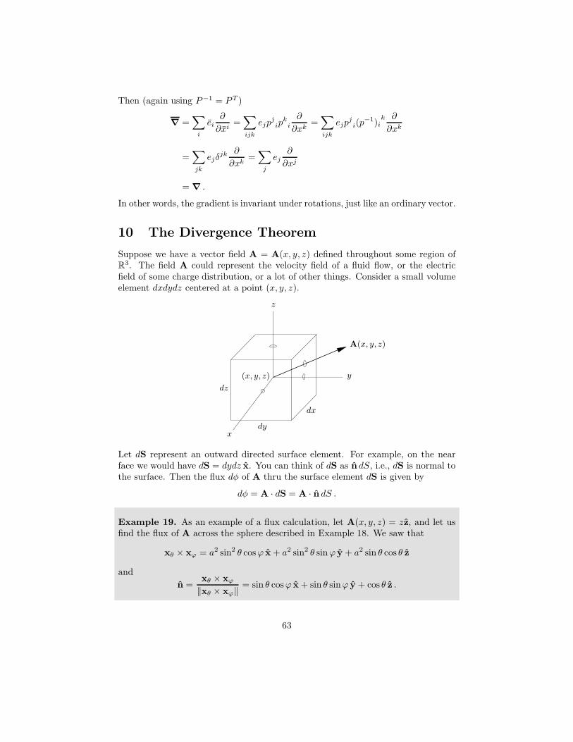
Then (again using P−1 = PT )

∇ =∑

i

ei∂

∂xi=∑

ijk

ejpjip

ki

∂

∂xk=∑

ijk

ejpji(p

−1)ik ∂

∂xk

=∑

jk

ejδjk ∂

∂xk=∑

j

ej∂

∂xj

= ∇ .

In other words, the gradient is invariant under rotations, just like an ordinary vector.

10 The Divergence Theorem

Suppose we have a vector field A = A(x, y, z) defined throughout some region ofR3. The field A could represent the velocity field of a fluid flow, or the electricfield of some charge distribution, or a lot of other things. Consider a small volumeelement dxdydz centered at a point (x, y, z).

x

y

z

dx

dy

dz

(x, y, z)

A(x, y, z)

Let dS represent an outward directed surface element. For example, on the nearface we would have dS = dydz x. You can think of dS as n dS, i.e., dS is normal tothe surface. Then the flux dφ of A thru the surface element dS is given by

dφ = A · dS = A · n dS .

Example 19. As an example of a flux calculation, let A(x, y, z) = zz, and let usfind the flux of A across the sphere described in Example 18. We saw that

xθ × xϕ = a2 sin2 θ cosϕ x + a2 sin2 θ sin ϕ y + a2 sin θ cos θ z

and

n =xθ × xϕ

‖xθ × xϕ‖= sin θ cosϕ x + sin θ sinϕ y + cos θ z .

63

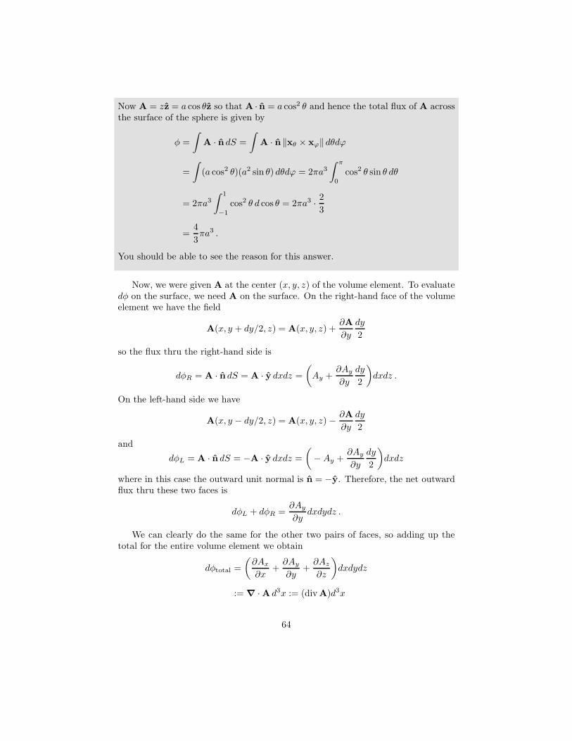
Now A = zz = a cos θz so that A · n = a cos2 θ and hence the total flux of A acrossthe surface of the sphere is given by

φ =

∫A · n dS =

∫A · n ‖xθ × xϕ‖ dθdϕ

=

∫(a cos2 θ)(a2 sin θ) dθdϕ = 2πa3

∫ π

0

cos2 θ sin θ dθ

= 2πa3

∫ 1

−1

cos2 θ d cos θ = 2πa3 · 2

3

=4

3πa3 .

You should be able to see the reason for this answer.

Now, we were given A at the center (x, y, z) of the volume element. To evaluatedφ on the surface, we need A on the surface. On the right-hand face of the volumeelement we have the field

A(x, y + dy/2, z) = A(x, y, z) +∂A

∂y

dy

2

so the flux thru the right-hand side is

dφR = A · n dS = A · y dxdz =

(Ay +

∂Ay

∂y

dy

2

)dxdz .

On the left-hand side we have

A(x, y − dy/2, z) = A(x, y, z) − ∂A

∂y

dy

2

and

dφL = A · n dS = −A · y dxdz =

(− Ay +

∂Ay

∂y

dy

2

)dxdz

where in this case the outward unit normal is n = −y. Therefore, the net outwardflux thru these two faces is

dφL + dφR =∂Ay

∂ydxdydz .

We can clearly do the same for the other two pairs of faces, so adding up thetotal for the entire volume element we obtain

dφtotal =

(∂Ax

∂x+

∂Ay

∂y+

∂Az

∂z

)dxdydz

:= ∇ ·A d3x := (div A)d3x

64

where this expression defines the divergence of the vector field A. So what div A

represents is the outward flux of A per unit volume.If we have a large volume, then we break it up into infinitesimal volume elements

and note that the contribution to the common interior faces will cancel. Then thetotal flux out of the bounding surface is given by

φtotal =

∫d3x∇ ·A .

On the other hand, we see from dφ = A · n dS that the total flux is also given by

φtotal =

∫A · n dS .

Equating these two expressions yields the Divergence Theorem:

Theorem 19. Let V be a volume in R3 with outward oriented bounding surface S.If A is a vector field defined over V with continuous first partial derivatives on anopen set containing V , then

∫

V

d3x∇ · A =

∫

S

A · n dS .

While we haven’t given a careful definition of orientation, for our purposes wetake it as an intuitively clear concept.

11 Stokes’ Theorem

Stokes’ Theorem is probably the most important of all vector integral theorems. Infact, in its most general form (which is formulated in terms of differential forms ona manifold, and is beyond the scope of these notes) it includes the classical Green’stheorem and the divergence theorem as special cases. We begin with a discussionof line integrals in R3.

Suppose we have a vector field

A(x, y, z) = Ax(x, y, z)x + Ay(x, y, z)y + Az(x, y, z)z

and a line element dr = xdx+ ydy + zdz. Then the line integral of A along a curveC is defined by

∫

C

A · dr =

∫

C

Ax(x, y, z)x + Ay(x, y, z)y + Az(x, y, z)z .

65

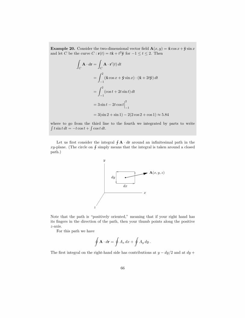
Example 20. Consider the two-dimensional vector field A(x, y) = x cosx+ y sin xand let C be the curve C : r(t) = tx + t2y for −1 ≤ t ≤ 2. Then

∫

C

A · dr =

∫

C

A · r′(t) dt

=

∫ 2

−1

(x cosx + y sin x) · (x + 2ty) dt

=

∫ 2

−1

(cos t + 2t sin t) dt

= 3 sin t − 2t cos t∣∣∣2

−1

= 3(sin 2 + sin 1) − 2(2 cos 2 + cos 1) ≈ 5.84

where to go from the third line to the fourth we integrated by parts to write∫t sin t dt = −t cos t +

∫cos t dt.

Let us first consider the integral∮

A · dr around an infinitesimal path in thexy-plane. (The circle on

∮simply means that the integral is taken around a closed

path.)

x

y

z

dx

dy

A(x, y, z)

Note that the path is “positively oriented,” meaning that if your right hand hasits fingers in the direction of the path, then your thumb points along the positivez-axis.

For this path we have

∮A · dr =

∮Ax dx +

∮Ay dy .

The first integral on the right-hand side has contributions at y − dy/2 and at dy +

66

dy/2:

∮Ax dx = Ax(x, y − dy/2, z) dx− Ax(x, y + dy/2, z) dx

=

[Ax(x, y, z) − ∂Ax

∂y

dy

2

]dx −

[Ax(x, y, z) +

∂Ax

∂y

dy

2

]dx

= −∂Ax

∂ydydx

where the (−) sign between the two terms in the first line is because along the toppath we have dr = −dx x. Similarly,

∮Ay dy = −Ay(x − dx/2, y, z) dy + Ay(x + dx/2, y, z)

=∂Ay

∂xdxdy

so that ∮A · dr =

(∂Ay

∂x− ∂Ax

∂y

)dxdy .

We now define the “vector” ∇ × A by

∇ × A =

(∂Az

∂y− ∂Ay

∂z

)x +

(∂Ax

∂z− ∂Az

∂x

)y +

(∂Ay

∂x− ∂Ax

∂y

)z

=

∣∣∣∣∣∣∣

x y z

∂/∂x ∂/∂y ∂/∂z

Ax Ay Az

∣∣∣∣∣∣∣

or

(∇ × A)i = εijk ∂

∂xjAk .

The quantity ∇ × A is called the curl of A, and is frequently written curlA. If∇ × A = 0, then we say that A is irrotational, and because of this, curlA issometimes called rotA.

Returning to our integral above, we have dxdy = ‖dS‖ where dS = z dS, andhence we can write our result in the form

∮A · dr = (∇ × A) · dS. This result

was derived for an infinitesimal element of area in the xy-plane. What about otherorientations of the area element? Well, we have shown that the gradient transformslike a vector under rotations, as does the cross product of two vectors. This meansthat the curl behaves like a vector. But we also know that the scalar product oftwo vectors is a scalar, and thus

∮A · dr = (∇ × A) · dS

67

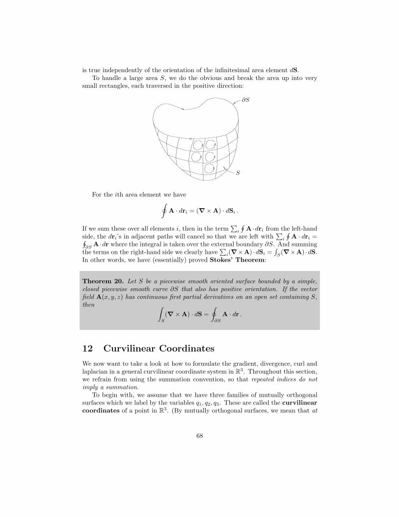
is true independently of the orientation of the infinitesimal area element dS.To handle a large area S, we do the obvious and break the area up into very

small rectangles, each traversed in the positive direction:

∂S

S

For the ith area element we have∮

A · dri = (∇ × A) · dSi .

If we sum these over all elements i, then in the term∑

i

∮A ·dri from the left-hand

side, the dri’s in adjacent paths will cancel so that we are left with∑

i

∮A · dri =∮

∂SA ·dr where the integral is taken over the external boundary ∂S. And summing

the terms on the right-hand side we clearly have∑

i(∇×A) ·dSi =∫

S(∇×A) ·dS.

In other words, we have (essentially) proved Stokes’ Theorem:

Theorem 20. Let S be a piecewise smooth oriented surface bounded by a simple,closed piecewise smooth curve ∂S that also has positive orientation. If the vectorfield A(x, y, z) has continuous first partial derivatives on an open set containing S,then ∫

S

(∇ × A) · dS =

∮

∂S

A · dr .

12 Curvilinear Coordinates

We now want to take a look at how to formulate the gradient, divergence, curl andlaplacian in a general curvilinear coordinate system in R3. Throughout this section,we refrain from using the summation convention, so that repeated indices do notimply a summation.

To begin with, we assume that we have three families of mutually orthogonalsurfaces which we label by the variables q1, q2, q3. These are called the curvilinear

coordinates of a point in R3. (By mutually orthogonal surfaces, we mean that at

68

each point in the region under consideration, the three coordinate curves intersectin a mutually orthogonal manner.)

Let there be an infinitesimal region under consideration, and let dli be an el-ement of length perpendicular to the surface qi = const. The length dli is reallythe distance between surfaces at qi and qi + dqi in the infinitesimal region underconsideration, and in general can be written in the form

dli = hidqi

where hi is in general a function of the coordinates q1, q2, q3.We also have the three unit vectors ui defined by (see Section 8)

ui =∂x/∂qi

‖∂x/∂qi‖.

Each ui is orthogonal to the surface of constant qi. (For example, think of x asbeing orthogonal to a surface of constant x.) However, be sure to realize thattheir orientation in space depends on their location, except in the particular caseof rectangular coordinates. Thus a general displacement dx can be written

dx = dl1u1 + dl2u2 + dl3u3

= h1dq1u1 + h2dq2u2 + h3dq3u3

and the volume element is dl1dl2dl3 or

d3x = h1h2h3dq1dq2dq3 .

If we write dli = hidqiui, then recalling the scalar triple product defined in Section2, we can write

d3x = Vol(dl1, dl2, dl3) = |(h1dq1u1 × h2dq2u2) · (h3dq3u3)|

=

∣∣∣∣∣∣∣

h1dq1 0 0

0 h2dq2 0

0 0 h3dq3

∣∣∣∣∣∣∣

= h1h2h3dq1dq2dq3 .

Now suppose we have a scalar function f = f(q1, q2, q3). Then its differential isgiven by

df =∂f

∂q1dq1 +

∂f

∂q2dq2 +

∂f

∂q3dq3 .

But dqi = (1/hi)dli so we have

df =1

h1

∂f

∂q1dl1 +

1

h2

∂f

∂q2dl2 +

1

h3

∂f

∂q3dl3

69

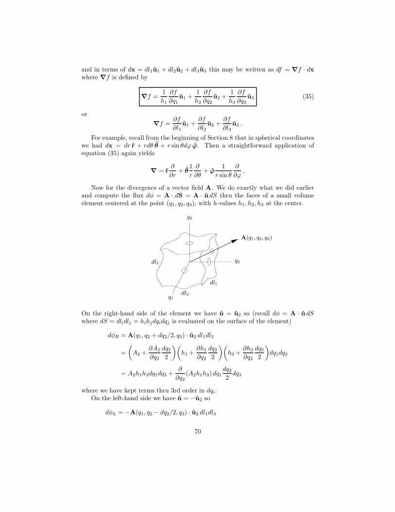
and in terms of dx = dl1u1 + dl2u2 + dl3u3 this may be written as df = ∇f · dxwhere ∇f is defined by

∇f =1

h1

∂f

∂q1u1 +

1

h2

∂f

∂q2u2 +

1

h3

∂f

∂q3u3 (35)

or

∇f =∂f

∂l1u1 +

∂f

∂l2u2 +

∂f

∂l3u3 .

For example, recall from the beginning of Section 8 that in spherical coordinateswe had dx = dr r + rdθ θ + r sin θdϕ ϕ. Then a straightforward application ofequation (35) again yields

∇ = r∂

∂r+ θ

1

r

∂

∂θ+ ϕ

1

r sin θ

∂

∂ϕ.

Now for the divergence of a vector field A. We do exactly what we did earlierand compute the flux dφ = A · dS = A · n dS thru the faces of a small volumeelement centered at the point (q1, q2, q3), with h-values h1, h2, h3 at the center.

q1

q2

q3

dl1

dl2

dl3

A(q1, q2, q3)

On the right-hand side of the element we have n = u2 so (recall dφ = A · n dSwhere dS = dlidlj = hihjdqidqj is evaluated on the surface of the element)

dφR = A(q1, q2 + dq2/2, q3) · u2 dl1dl3

=

(A2 +

∂A2

∂q2

dq2

2

)(h1 +

∂h1

∂q2

dq2

2

)(h3 +

∂h3

∂q2

dq2

2

)dq1dq3

= A2h1h3dq1dq3 +∂

∂q2(A2h1h3) dq1

dq2

2dq3

where we have kept terms thru 3rd order in dqi.On the left-hand side we have n = −u2 so

dφL = −A(q1, q2 − dq2/2, q3) · u2 dl1dl3

70

= −(

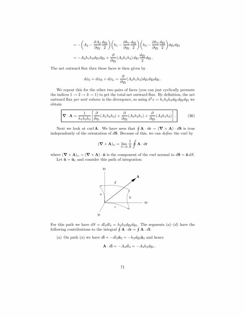
A2 −∂A2

∂q2

dq2

2

)(h1 −

∂h1

∂q2

dq2

2

)(h3 −

∂h3

∂q2

dq2

2

)dq1dq3

= −A2h1h3dq1dq3 +∂

∂q2(A2h1h3) dq1

dq2

2dq3 .

The net outward flux thru these faces is then given by

dφ2 = dφR + dφL =∂

∂q2(A2h1h3)dq1dq2dq3 .

We repeat this for the other two pairs of faces (you can just cyclically permutethe indices 1 → 2 → 3 → 1) to get the total net outward flux. By definition, the netoutward flux per unit volume is the divergence, so using d3x = h1h2h3dq1dq2dq3 weobtain

∇ ·A =1

h1h2h3

[∂

∂q1(A1h2h3) +

∂

∂q2(A2h3h1) +

∂

∂q3(A3h1h2)

]. (36)

Next we look at curlA. We have seen that∮

A · dr = (∇ × A) · dS is trueindependently of the orientation of dS. Because of this, we can define the curl by

(∇ × A)n = limS→0

1

S

∮A · dr

where (∇ ×A)n = (∇ × A) · n is the component of the curl normal to dS = n dS.Let n = u1 and consider this path of integration:

q1

q2

q3

A

ab

c

d

For this path we have dS = dl2dl3 = h2h3dq2dq3. The segments (a)–(d) have thefollowing contributions to the integral

∮A · dr =

∮A · dl:

(a) On path (a) we have dl = −dl3u3 = −h3dq3u3 and hence

A · dl = −A3dl3 = −A3h3dq3 .

71

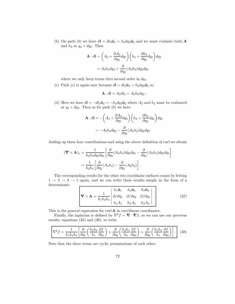
(b) On path (b) we have dl = dl3u3 = h3dq3u3 and we must evaluate both A

and h3 at q2 + dq2. Then

A · dl =

(A3 +

∂A3

∂q2dq2

)(h3 +

∂h3

∂q2dq2

)dq3

= A3h3dq3 +∂

∂q2(A3h3)dq2dq3

where we only keep terms thru second order in dqi.

(c) Path (c) is again easy because dl = dl2u2 = h2dq2u2 so

A · dl = A2dl2 = A2h2dq2 .

(d) Here we have dl = −dl2u2 = −h2dq2u2 where A2 and h2 must be evaluatedat q3 + dq3. Then as for path (b) we have

A · dl = −(

A2 +∂A3

∂q3dq3

)(h2 +

∂h2

∂q3dq2

)dq2

= −A2h2dq2 −∂

∂q3(A2h2)dq2dq3

Adding up these four contributions and using the above definition of curl we obtain

(∇ × A)1 =1

h2h3dq2dq3

[∂

∂q2(A3h3)dq2dq3 −

∂

∂q3(A2h2)dq2dq3

]

=1

h2h3

[∂

∂q2(A3h3) −

∂

∂q3(A2h2)

].

The corresponding results for the other two coordinate surfaces comes by letting1 → 2 → 3 → 1 again, and we can write these results simply in the form of adeterminant:

∇ × A =1

h1h2h3

∣∣∣∣∣∣∣

h1u1 h2u2 h3u3

∂/∂q1 ∂/∂q2 ∂/∂q3

h1A1 h2A2 h3A3

∣∣∣∣∣∣∣. (37)

This is the general expression for curlA in curvilinear coordinates.Finally, the laplacian is defined by ∇2f = ∇ · ∇f , so we can use our previous

results, equations (35) and (36), to write

∇2f =1

h1h2h3

[∂

∂q1

(h2h3

h1

∂f

∂q1

)+

∂

∂q2

(h3h1

h2

∂f

∂q2

)+

∂

∂q3

(h1h2

h3

∂f

∂q3

)]. (38)

Note that the three terms are cyclic permutations of each other.

72