Embed Size (px)
Citation preview

1
Supply & Use Tables for Ireland 2016
This explanatory note is provided by the CSO to users of our annual Supply & Use Tables. It also describes the Input-Output Tables which are available every five years. It includes descriptive material which we hope will aid our users understanding of the range of tables available. The note touches on table structure and compilation as well as highlighting the potential of these tables in providing insights for economic analysis. An accompanying ‘Overview’ set of slides/notes, covering the same areas, is provided as a visual reference guide and summary for users.
Supply & Use and Input-Output Tables are a useful method for linking microeconomic and macroeconomic analysis. They provide a detailed picture of the transactions of goods and services by industries and consumers in the economy. They highlight the inter-industry flows that lie behind the National Accounts main aggregates.
The following note should be read in conjunction with Supply and Use Tables for Ireland 2016
published by the Central Statistics Office (CSO). This can be found on the CSO website:
http://www.cso.ie/en/statistics/nationalaccounts/
This working note is mostly based on material produced for a seminar delivered to the Irish
Government Economic & Evaluation Service (IGEES) in the Department of Finance. It uses some
additional material from the UK Office for National Statistics and the Scottish Government. Any
views expressed are those of the authors (Eóin Flaherty and Mark Manto) and do not necessarily
reflect the views of the CSO.

2
Contents Introduction ............................................................................................................................................ 3
Supply Table at basic prices (Table 1) ..................................................................................................... 7
Use Table at purchasers’ prices (Table 2) ............................................................................................. 11
Consistency of Supply & Use Tables with the National Accounts ........................................................ 14
Gross Value Added/Gross Domestic Product in Supply & Use tables .................................................. 16
Data sources .......................................................................................................................................... 18
Balancing ............................................................................................................................................... 19
Supply & Use Tables in previous year prices (Tables 3 and 4) .............................................................. 21
Intermediate Tables .............................................................................................................................. 27
Input-Output Tables .............................................................................................................................. 29
Multipliers ............................................................................................................................................. 32
List of abbreviations and acronyms ...................................................................................................... 35

3
Introduction
Why Supply & Use and Input-Output Tables?
Before we begin, let’s put these tables in some sort of context by asking three simple questions.
• Why are they produced?
• What is produced?
• When are they produced?
Why are they produced?
The short answer is because Ireland is legally obliged, under European regulation, to produce these
tables. Failure to fulfil such legally binding obligations would result in Ireland, through the CSO,
receiving warnings and possible financial penalties from the European Commission. Such penalties
can be levied at a daily rate.
Most CSO releases and publications (perhaps 80% plus, and possibly 90% plus in the
macroeconomics area) are required under European legislation. These requirements, particularly
since the introduction of the EMU and also in light of the Great Recession, have increased
significantly in the macroeconomic area.
These tables were required under ESA1995 (European System of Accounts) which was, from the
2014 production cycle, superseded by ESA2010. From a Supply & Use perspective there were some
differences in the table production requirements, but it was methodological changes which were
most evident to National Accounts users. This was partly through the incorporation of greater
estimates for the shadow economy, some changes to FISIM, but it was most evident from an Irish
perspective in the capitalisation of Research and Development (R&D).
What is produced?
Ireland is obliged to produce annual Supply and Use Tables (S&UT) in both current and previous year
prices (PYP). The latest Supply and Use Tables describe 2016 and were published in 2019. The Supply
and Use Tables are ESA Tables 1500 and 1600 respectively. Every five years, Ireland is also required
to produce Input-Output Tables (I/O). These are for reference years ending in a 5 or a 0. These Input-
Output Tables comprise the total, domestic and imported Input-Output tables (ESA Tables 1700,
1800 and 1900 respectively). The latest Input-Output Tables describe 2015 and were published in
2018. All tables have used the NACE Rev. 2 classification since the 2008 tables.
As well as these 7 tables (2 S&UT in current prices, 2 S&UT in PYP and 3 I/O) there are also 5 other
obligatory. These are ESA tables 1610 (Use table at basic prices), 1611 (Use table for domestic
products), 1612 (Use table for imported products), 1620 (Use table for margins), 1630 (taxes minus
subsidies on products). Note that the pair of tables of specific interest to many of our domestic
users, Table 11 (Coefficient table) and Table 12 (Leontief inverse), are not ESA tables – either
required or voluntary. CSO produce these tables because we know that they will be of interest and
benefit for many of our users.
There is another element to the Supply & Use ESA requirements, which we touched on above. These
are the constant price tables. They are calculated in previous year prices (PYP). This allows for real,
or volume, changes to be measured at a very detailed level across the economy. Detailed price

4
changes are also revealed in these tables. These different changes, rather than just having value or
nominal changes, can provide great insights into the changing structure and competiveness of
specific sectors of the economy as well as highlighting shifting patterns of growth and its
consequences. We will discuss these PYP tables in more detail later.
All of the above tables are available on the CSO website. See the following webpage for the latest
national accounts releases and publications, including Supply & Use and Input-Output Tables:
http://www.cso.ie/en/statistics/nationalaccounts/
The following page provides a link to the archived national accounts releases and publications:
http://www.cso.ie/en/statistics/nationalaccounts/archive/
When are they produced?
All S&UT are produced on an n+3 timeline. For example, the latest 2016 S&UT, compiled in ESA2010,
and which were published nationally in 2018 were also transmitted to Eurostat at the same time.
Eurostat examine and publish these tables. The 2009 S&UT were published in March 2013. For the
2010 tables this was improved to January and has been incrementally improved through efficiencies
each subsequent year allowing the CSO to achieve near simultaneous publication with Eurostat
transmission and validation, so the tables are now also published domestically within the n+3 year.
The Census of Industrial Production (CIP) and the Annual Services Inquiry (ASI) are two of the main
data sources used in the creation of these tables (we will talk more about these and some of the
other main data sources later). Both of these are generally published with at least an n+18 month
lag. For example, the latest CIP and ASI publicly available (as of September 2019) both describe 2016
and were published in September 2018.
Overview of table structure
There were four transaction tables in the 2016 publication of October 2019. These were:
• Table 1 Supply Table at basic prices (product by industry)
• Table 2 Use Table at purchasers’ prices (product by industry)
• Table 3 Supply Table at previous year prices (product by industry)
• Table 4 Use Table at previous year prices (product by industry)
(NOTE: Users might find it beneficial to have a hard copy of the following tables to hand for reference
purposes while reading this text. These can be found on the CSO website.)
Considered together, the Supply and Use and symmetric Input-Output tables give a detailed picture
of the transactions of all goods and services by industries and final consumers in the Irish economy
in a single year. They serve as an integrated framework for all production statistics and are used as a
statistical tool to compile and reconcile independent estimates of National Accounts aggregates.
The Supply and Use framework shows the components of gross value added (GVA) by industry as
well as imports, exports and taxes and subsidies on products. The GVA in the Use table measures the
contribution to GDP made by each particular industry branch.

5
Note on classifications used in S&UT
NACE (Nomenclature des Activités Économiques dans la Communauté Européenne) is a European
industry standard classification system. NACE is the acronym used to designate the various statistical
classifications of economic activities developed since 1970 in the European Union (EU). NACE
provides the framework for collecting and presenting a large range of statistical data according to
economic activity in the fields of economic statistics (e.g. production, employment, national
accounts) and in other statistical domains. Statistics produced on the basis of NACE are comparable
at European and, in general, at world level. The use of NACE is mandatory within the European
statistical system.
CPA (Classification of Products by Activity) is the classification of products (goods as well as services)
at the level of the European Union (EU). Product classifications are designed to categorize products
that have common characteristics. They provide the basis for collecting and calculating statistics on
the production, distributive trade, consumption, international trade and transport of such products.
CPA product categories are related to activities as defined by the Statistical classification of
economic activities in the European Community (NACE). Each CPA product - whether a transportable
or non-transportable good or a service - is assigned to one single NACE activity. This linkage to NACE
activities gives the CPA a structure parallel to that of NACE at all levels.
For convenience I will refer throughout the note to NACE industry and NACE product.
A modern open economy engages in four basic economic activities:
1. Production (industries produce goods and services)
2. Consumption (purchases of goods and services)
3. Accumulation (capital transactions, i.e. fixed investment expenditure and changes in stocks)
4. Trade (imports and exports)
Measurements of all four activities are captured in the framework of the Supply & Use Tables. The
resulting tables serve a number of purposes, all of which contribute in different ways to
understanding the economy.
We can think of the economy as a series of relationships. We can create flow diagrams of different
elements of these relationships. For example in economics the reciprocal circulation of income
between producers and consumers is referred to as the circular flow of income. The circular flow of
income shows how financial payments flow between corporations and households within the
economy. It also shows the interaction between different sectors of the economy and the rest of the
world. An overview of these interactions is presented below1. The strength and value of the Supply
& Use tables is that all such relationships are described in the tables, covering all aspects of the
economy. Such a set of holistic and comparable tables enable these relationships to be unpicked and
examined discretely element by element, sector by sector.
1 Diagram from ONS. The arrows in the diagram show the flow of money between the different institutions as a result of transactions between them.

6

7
Supply Table at basic prices (Table 1)
The Supply table – what do we mean by supply?
The Supply table provides estimates of the supply of goods
and services (products) by domestic industries as well as
imports of goods and services. The supply of products is
presented in the rows while the columns show the industry
branches that produce these goods and services. Each
industry is classified according to whichever product accounts
for the largest part of its output. Its principal production,
shown on the diagonal elements of the Supply table, is
therefore larger than its secondary production shown on the
off-diagonal elements. So if we read the Supply table down,
i.e. an industry column, the bottom line of the Supply table is
the output of that industry – i.e. the total output of that industry irrespective of what products that
output might be composed. Similarly if we read across the rows, we see in the right hand column the
total supply of that particular product.
A summary of the 2016 Supply table is shown below.
Do we see a pattern in the domestic supply matrix?
Yes we do. If we think of a simple item like a pen, then we can ask what is the total supply of pens in
Ireland? Reading across the relevant row (in this case pens are in NACE 32.99) total supply at basic
prices = pens made in Ireland (domestic supply) plus imported pens. This will also be total demand.
As we mentioned above, not all pens need necessarily be made by NACE 32 industry, there may be
secondary production.
What do we mean by secondary production?
Individual firms and organisations are classified according to the products they make. If they
produce more than one product, they are classified according to whichever product accounts for the
largest component part of their output (€). Each industry produces what is termed to be its principal
product (shown in the diagonal elements in the table) and many industries also produce a range of
other products referred to as secondary production (shown in the off-diagonal cells) or by-products.
What we see in the domestic supply matrix then is that generally (but not always) the bulk of the
output of a particular product is by the corresponding industry.
8
Take the example of industry NACE 16 (Wood and wood products). We can see that in 2016 the
output of NACE 16 industry was €887 million of which €859 million was NACE 16 product. NACE 16
industry also produces a small quantity of other products, for example €11 million of NACE 17 (Pulp,
paper and paper products), €5 million of NACE 22 (Rubber and plastics), etc. Switching to NACE 16
product, we see that the total domestic supply was €894 million, of which (as we saw above) the
large majority (€859 million) was produced by NACE 16 industry. NACE 16 product was also
produced by NACE 1-3 industry, NACE 17, NACE 25, etc.
Why are these of interest?
The diagonal versus off-diagonal figures are of interest because they show not just the diversity of
output within each industry, but the competition which can exist not just within an industry but
across apparently different industries.
Examples of the how the Supply Table can be used are as follows:
1. Indicators of the diversity of commodities produced by an industry. The leading diagonal of the
supply table shows the value of output of an industry’s principal product. This can be presented as
'Principal Products as a percentage of Total Industry Output'.
2. Indicators of market share. Conversely, it is possible to look at the industries that produce
particular products, e.g. to examine the share of manufactured products produced by the
manufacturing industry. This is an indicator of market share and can be presented, at detailed
industry level, in the Supply Table as 'Principal Products as a percentage of Total Output of Products'.
3. Indicators of import penetrations. This is the share of the total supply of a product.
The Supply table is described as being at basic prices, but the final column on the right
describes total Supply at purchasers’ prices. What is the difference?
The sum of these two figures (domestic supply and the imports column) is total supply at basic
prices. We see that the right hand side of the Supply table is valued at purchasers’ prices.
This transition occurs through the addition of distributors’ trading margins and taxes less subsidies
on production. Distributors’ trading margins represent the difference between the prices at which
distributors buy and sell their products.
Another way of thinking about it is as the difference between the actual or imputed sale price
realised on a good purchased for resale and the price that would have to be paid by the distributor
to replace the good at the time it is sold.
In the domestic supply table, these trading margins are shown as the output of the distribution
industries, in the corresponding distribution services’ product rows. In the distributors’ trading
margin column of the supply table, the trading margins are distributed among the goods actually
traded, and deducted from the distribution services products, so that the total for this column is
zero. Taxes on products include VAT and excise duties. The addition of these product taxes and the
subtraction of product subsidies complete the transition from basic prices to purchasers’ prices.

9
More detail on the treatment of the motor trade, retail and wholesale
The outputs of the distribution sector are defined in a special way for national accounts purposes
and may not be as expected. The motor trade, retail and wholesale activities are regarded as
producing a service which is measured as the price at which their products are sold minus the
purchase price of these products (which they purchased for direct resale). This is referred to as the
gross margin. Thus the retail supermarket is not regarded as providing food or drink nor is the
drapery outlet regarded as providing clothes. In the Supply and Use framework, the food and clothes
are the products of their respective industries or are imported and retailers are regarded as
providing a sales service (see the distribution rows 45 – 47 of the Supply table).
The gross margin is also used to measure the output of distribution activity by firms that are mainly
involved in another activity such as manufacturing.
More detail on valuation and the difference between basic price and purchasers’
prices
The values of the domestically produced products in the Supply table are shown initially at basic
prices while they are transformed to purchasers’ prices in the final columns. Imports are shown at
c.i.f. (cost, insurance and freight inclusive) prices as in the published merchandise trade statistics.
The basic price is the price receivable by the producer for a unit of a good or service produced,
minus any tax payable as a consequence of its production or sale (i.e. taxes on products), plus any
subsidy receivable on that unit as a consequence of its production or sale (i.e. subsidies on
products). Thus the basic price excludes the well-known product taxes such as VAT, excise duties,
import duties, etc. In theory, the basic price excludes any transport charges invoiced separately by
the producer but includes any transport charges charged on the same invoice. It does not include
any trade margin. The basic price measures the amount retained by the producer and is therefore
the price most relevant for the producer’s decision making.
The purchaser’s price is the price the purchaser actually pays for the product including any taxes less
subsidies on the product (but excluding deductible taxes). The conversion from basic prices to
purchasers’ prices involves distributing the trade margins of retailers and wholesalers among the
products on which they are charged. The margin in the motor trade and domestic wholesale and
retail trades appears as negative values in rows 45 to 47 of the trade margin column of the Supply
table as these margins are distributed in the same column among the products on which they fall.
Valuation of imports in the NIE and in the Trade statistics
Merchandise imports are valued as c.i.f. (cost, insurance and freight) in the Trade statistics, while
they are valued as f.o.b. (free on board) in the annual National income and Expenditure (NIE). Cost,
insurance and freight (c.i.f.) requires the seller to arrange for the carriage of goods by sea to a port
of destination, and provide the buyer with the documents necessary to obtain the goods from the
carrier. Free on board (f.o.b.) on the other hand requires the seller to deliver goods on board a
vessel designated by the buyer. The seller fulfils their obligations to deliver when the goods have
passed over the ship's rail. The different valuations require an adjustment to be made to move from
the detailed product figures in c.i.f. to match the f.o.b. total imports as shown in the NIE. For

10
consistency purposes, to ensure that the total supply of a product equals total use, a similar
adjustment is made to exports in the Use table.
Are all output totals for each sector in the Supply tables measured the same way?
No. There are three specific areas of interest here. First, most of the output of government is non-
market output, and cannot be identified as uses of any specific institutional sector. Conventionally,
this non-market output is valued according to the sum of the inputs used in its production (pay,
procurement, gross operating surplus). The sum of these costs, when added to the value of market
output and own-account production, goes into the relevant industry column of the supply table. As
there is assumed to be no net operating surplus on government activities, the gross operating
surplus element consists only of consumption of fixed capital. Second is imputed rent. This is the
amount an owner-occupier would need to pay to rent their own property. This affects NACE 68.
Third is FISIM. What is this? The output of the banking sector in the national accounts is called FISIM
(Financial Intermediation Services Indirectly Measured). For borrowing from banks, this is essentially
the difference between the interest rate actually paid and what would have been paid at a reference
rate (such as the ECB’s base rate). For deposits with banks, it is the difference between the interest
actually received and what would have been received had the deposits received interest at the
reference rate. All sectors of the economy can pay FISIM. So, in principle, the levels of bank deposits
and borrowing are needed by sector and industry, split by country of residence of the bank. This
information is not readily available.

11
Use Table at purchasers’ prices (Table 2)
The Use table – what do we mean by
use?
The structure of the Use table is more
complicated than the Supply table. Where the
Supply Table presented the supply of goods
and services for consumption, the Use Table
shows the demand for the goods and services
by industries and final demand across the
product rows.
We can generalise output as being of one of
three types: output for final domestic use,
output for export, and output used for
intermediate use. All three types of use are
captured in the Use table.
The Use table shows the use of products by domestic industry and by the final demand sectors, i.e.
consumption by households, government, non-profit organisations serving households (NPISH),
capital formation (GFCF) and export. As in the previous table, industries are shown in the columns
and products in the rows. Thus the columns of figures for industries NACE 1 - 97 show the goods and
services used by each industry for the purposes of achieving its output. The purchases in these
columns relate to intermediate consumption only. Capital purchases are shown separately. All the
purchases of households in their private (non-business) capacity as consumers are included under
household consumption with the exception of the purchase of dwellings, which is included with
capital formation.
A summary of the 2016 Use table at purchasers’ prices is shown below.
Additional information for each industry is shown at the end of the industry columns where
estimates of the primary inputs, which are the components of the gross value added (GVA) by each
industry, are provided. This is the Income method of calculation of GVA. These are in the form of

12
compensation of employees (COE), non-product (i.e. overhead) taxes and subsidies, net operating
surplus (NOS or profits) and consumption of capital (or depreciation) (CFC). The latter two items,
when combined, are referred to as gross operating surplus (GOS). The sum of these rows is referred
to as the gross value added of the industry and is equal to the output of the industry minus its
intermediate consumption costs, which is the Output method of calculation of GVA.
What are the different elements within the Use table?
If the domestic output part of the Supply Table at basic prices can be thought of as showing the
composition of industries’ outputs by product, the left hand side of the Use Table can be thought of
as showing the composition of industries’ inputs.
Similarly inter-industry use can be thought of as being either the intermediate consumption of
imports or of domestic supply, for both of which the resulting output may be one of the three
options previously listed. In later tables (Table 4 and Table 5) we split the Use table into domestically
produced and imported inputs).
The Use Table can be split into three main sections.
• Inter-industry use shows the inputs of products, both domestic and imported, used by
industries in the production of their output.
• Final use shows the purchases of each product by each category of final demand (e.g.
consumers, government, exports).
• Primary inputs are employees' salaries, taxes less subsidies on production and gross
operating surplus (=consumption of fixed capital and net operating surplus), which together
constitute Gross Value Added calculated by the Income method.
What is Intermediate demand?
The columns shown in the intermediate demand part of the table list the goods and services each
industry uses in order to produce its output (as described by the corresponding industry column in
the Supply Table). The column totals give the total intermediate consumption of each industry. The
row totals give the total intermediate demand for each product category.
What are the Primary inputs?
The difference between the value of industry output at basic prices (which are the column totals of
the Supply table) and the value of industry intermediate consumption at purchasers’ prices is Gross
Value Added (GVA), which is treated as an input in the Supply and Use framework. GVA itself can be
split into three aggregate components: Taxes less Subsidies on Production, Compensation of
Employees, and Gross Operating Surplus (including capital consumption). These make up the
Primary Inputs table, which appears below the intermediate consumption part of the Use Table so
that the column totals by industry in the Use Table sum to total output by industry.
If we add the industry intermediate consumption figure to the GVA figure we should get the same
output figure we saw in the Supply table. Again if we take the example of NACE 16, the industry
output from the Supply table in 2016 was €887 million. Examining Table 2 NACE 16 industry, we see
that intermediate consumption was €659 million. COE was €154 million, NOS was €11 million, CFC
was €59 million while net taxes on production were €3 million. So GVA equals €228 million

13
(228=154+11+59+3). The implied Output from the Use table therefore equals the sum of €659
million plus €228 million = €887 million, which is as per the Supply table NACE 16 industry output.
What is Final demand?
The final demand section of the Use Table comprises the following components in the columns:
• Final Consumption Expenditure by: both resident and non-resident households (e.g. tourists
or business visitors); by Non-Profit Institutions Serving Households (NPISHs); and by
government (central and local combined).
• Gross Capital Formation, which is made up by Gross Fixed Capital Formation (commonly
called “investment expenditure”); Valuables; and Change in Inventories (which includes
work in progress);
• Exports of goods and services. A four-way breakdown of exports by geographical area: EU,
EMU, non-EMU and Rest of the World (RoW).
For each of these components, a breakdown of final demand by product is given in the rows.
Government consumption expenditure
Under the National Accounts framework, government activities are presented in such a way that it
appears to be the final consumer of its own non-market output, or put another way, government, on
behalf of the people, fund a range of activities across the public services. To reflect this, the column
for the final consumption expenditure of government appears in the final demand section of the Use
Table. These columns display the total other non-market output of government by product. They
equate to the row total of the other non-market component of the government Supply Tables.
For instance, consider industry 84, public administration and defence. In the Supply table all output
of this industry is allocated to the corresponding principal product. There is little or no market
output associated with this product, so the total intermediate consumption of this product is
relatively small. Therefore in order to balance the supply of this product with the demand for it,
government final consumption expenditure for this product itself almost equals total supply.
More detail on valuation
The purchases of the products in the Use table are valued at purchasers’ prices, which have already
been explained in the description of the Supply table above. There is no distinction in this table
between imported and home produced products. The gross value added of the industries shown in
the second last row, being equal to the output of the industries valued at basic prices minus their
intermediate consumption at purchasers’ prices is regarded as being valued at basic prices.

14
Consistency of Supply & Use Tables with the National Accounts
Are data in the Supply & Use tables consistent with the N.I.E.?
Yes they are consistent. The Supply & Use tables are consistent with the National Income and
Expenditure (NIE) totals of the year in question. Hence the NIE2018 published in July 2019 figure for
2016 imports (€285,882 million Item 84, Table 5) is consistent with the total imports figure (including
the cif/fob adjustment described above and expenditure outside the state) in the Supply table.
Similarly the taxes on products figure of €21,071 million and the subsidies on products figure of €934
million are consistent with the 2016 NIE2018 figures in Item 52 and Item 53 respectively in Table 3. A
detailed illustration of the Supply & Use Tables and NIE consistency is provided in the accompanying
‘Overview’ presentation. A table showing the consistency between the Supply and Use tables with
NIE aggregates is shown below.
Consistency of 2016 Supply and Use Tables with NIE18
Comparison with other CSO sources
Although the Supply and Use tables are consistent with national accounts data published in NIE2017
and thereby consistent with the overall balance of payments data compiled by the CSO, it is not
possible to achieve full agreement with all CSO publications. The exercise of compiling Supply and
Use tables helps to identify discrepancies that exist within different data sources. It is hoped that
some of these discrepancies will be removed over time.
There are four main reasons for differences that occur between the aggregates presented in the
Supply and Use tables and the aggregates presented in other publications, e.g. the Census of
Industrial Production (CIP) and Annual Services Inquiry (ASI). Some examples of are set out below.
Terminology
For the most part, the underlying definitions are consistent throughout CSO publications, but certain
differences do arise. For example, the output in the Supply table is inclusive of freight and of the
margin gained on goods resold without further processing. These two items may not be part of
‘gross output’ in the CIP. Also the term ‘compensation of employees’ in national accounts can

15
include the employer’s contribution to social insurance and other labour costs, which are not
included in the wages and salaries variable in the CIP and ASI.
Accounting practices
Some international sales by Irish companies are included in the CIP gross turnover but are treated on
a net basis (i.e. sales less purchases) in the balance of payments. This can arise particularly where
Irish companies sell products abroad which they have also purchased abroad. The products
purchased may never have come into Ireland or undergone any further processing following
purchase by the Irish enterprise. Supply and Use adjusts the CIP data and includes the net amount
as an export of a service. Conversely, there are companies manufacturing on a fee basis whose
transactions may be recorded gross in the international trade statistics. This can arise where
companies process goods for another company in their enterprise group abroad. The goods are
imported and exported and may therefore have been included in the merchandise trade statistics
although ownership of the goods did not change in the process. Generally in these cases the
merchandise trade is adjusted to convert the goods imported and exported to a fee based service
for use in the balance of payments and national accounts. In the case of telecommunications, some
of the turnover in the ASI arises from importing and exporting telecommunications services,
whereas balance of payments uses a net treatment. Supply and Use adopts the balance of payments
practice in these situations.
Classifications
Output by product may be classified differently in the Prodcom Inquiry to the export statistics. This
difficulty is corrected by realigning at a product level the production with the exports or vice versa.
Sometimes the classifications in the two systems are quite unrelated. For example, what appears in
one classification as a chemical may be classified in the other as food and beverages.
Conflicts in classification also occur at the overall activity level of companies. The company’s NACE
code in the national accounts and balance of payments may differ from the NACE code used by CIP
or ASI. Usually the classification used in the CIP or ASI is adopted in the Supply and Use tables. It can
also happen that the mismatch highlights a problem that is resolved by transferring the company
within the CIP or ASI.
Conflicting data
The Supply and Use tables are compiled using data from different sources. It is therefore not
surprising that there are occasional instances of contradictory and conflicting information. Some
examples are: the value of production by a company, measured in the CIP, may be less than their
exports, measured by the international merchandise trade statistics; the value added of a company,
measured by national accounts from administrative sources, may not concur with the same variable
derived in the CIP or the ASI; compensation of employees calculated in national accounts based on
employment figures can conflict with the wages and salaries figures in the CIP and ASI, which are
assembled from company data. Reconciliation of these types of problem can result in differences
between the variable presented in the Supply and Use tables and the same variable in the CIP or ASI.

16
Gross Value Added/Gross Domestic Product in Supply & Use tables This consistency of the Supply & Use Tables with the N.I.E. can be illustrated using the three
methods of calculating GVA/GDP. A detailed illustration of the Supply & Use Tables and calculation
of GVA/GDP is provided in the accompanying ‘Overview’ presentation.
Three methods of calculating GVA/GDP
An important feature of the Supply and Use framework is that it presents Gross Domestic Product as
measured using three distinct approaches. These are the Production method (also known as the
Output method), the Income method and the Expenditure method.
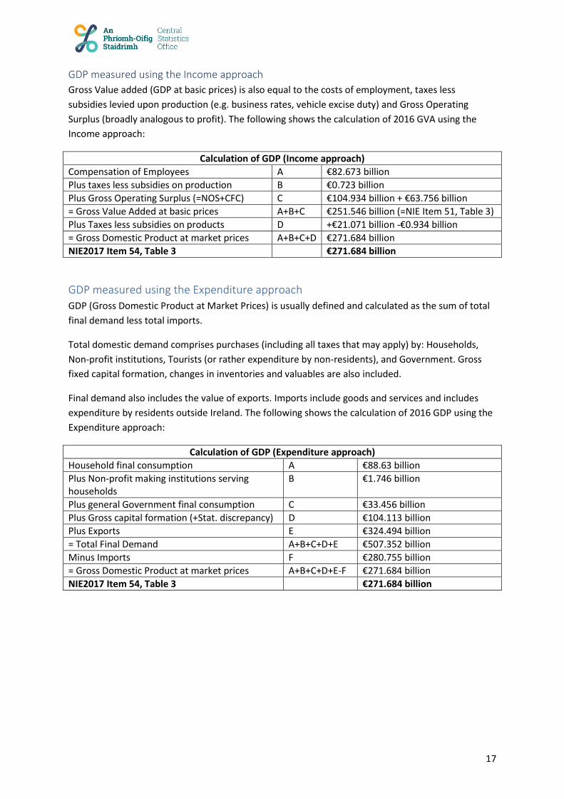
GDP measured using the Production approach
GDP at basic prices is also known as Gross Value Added (GVA); that is, it is a measure of the gross
value added to the economy by each producing unit. Broadly speaking, it is simply the sum of each
company’s outputs (sales) less inputs (purchases).
The output of an organisation is approximately equal to the total value of sales (turnover) over a
given period although account is also taken of goods manufactured but held in inventory and work in
progress as well as goods and services bought and resold without further processing. The final
component of output includes any items of a capital nature created in-house for the companies own
final use e.g. databases and other computer systems. These are valued and added to the other items
to form a figure for the total value of goods and services produced by an organisation - their Output
at Basic Prices.
In producing these outputs, an organisation will have to purchase raw materials, energy and other
intermediate inputs of goods and services: these are subtracted from the output (including any taxes
relating to these purchases) to yield Gross Value Added. It may be summarised as follows:
Output by Industry (from the Supply table) minus Intermediate consumption by Industry (from the
Use table) = GVA by Industry
The following shows the calculation of 2016 GVA using the Production approach, also known as the
Output approach:
Calculation of GDP (Production approach)
Total output at basic prices A €540.679 billion
Minus intermediate inputs at purchasers’ prices B €89.132 billion
= Gross Value Added at basic prices A-B €251.546 billion (=NIE Item 51, Table 3)
Plus Taxes less subsidies on products C +€21.071 billion -€0.934 billion
= Gross Domestic Product at market prices A-B+C €271.684 billion
NIE2017 Item 54, Table 3 €271.684 billion
17
GDP measured using the Income approach
Gross Value added (GDP at basic prices) is also equal to the costs of employment, taxes less
subsidies levied upon production (e.g. business rates, vehicle excise duty) and Gross Operating
Surplus (broadly analogous to profit). The following shows the calculation of 2016 GVA using the
Income approach:
Calculation of GDP (Income approach)
Compensation of Employees A €82.673 billion
Plus taxes less subsidies on production B €0.723 billion
Plus Gross Operating Surplus (=NOS+CFC) C €104.934 billion + €63.756 billion
= Gross Value Added at basic prices A+B+C €251.546 billion (=NIE Item 51, Table 3)
Plus Taxes less subsidies on products D +€21.071 billion -€0.934 billion
= Gross Domestic Product at market prices A+B+C+D €271.684 billion
NIE2017 Item 54, Table 3 €271.684 billion
GDP measured using the Expenditure approach
GDP (Gross Domestic Product at Market Prices) is usually defined and calculated as the sum of total
final demand less total imports.
Total domestic demand comprises purchases (including all taxes that may apply) by: Households,
Non-profit institutions, Tourists (or rather expenditure by non-residents), and Government. Gross
fixed capital formation, changes in inventories and valuables are also included.
Final demand also includes the value of exports. Imports include goods and services and includes
expenditure by residents outside Ireland. The following shows the calculation of 2016 GDP using the
Expenditure approach:
Calculation of GDP (Expenditure approach)
Household final consumption A €88.63 billion
Plus Non-profit making institutions serving households
B €1.746 billion
Plus general Government final consumption C €33.456 billion
Plus Gross capital formation (+Stat. discrepancy) D €104.113 billion
Plus Exports E €324.494 billion
= Total Final Demand A+B+C+D+E €507.352 billion
Minus Imports F €280.755 billion
= Gross Domestic Product at market prices A+B+C+D+E-F €271.684 billion
NIE2017 Item 54, Table 3 €271.684 billion

18
Data sources Main data sources used in construction of Supply & Use tables
We have previously mentioned that the main aggregates in the 2016 Supply and Use tables (value
added, final consumption, imports and exports, etc.) are consistent with the 2016 estimates shown
in the publication National Income and Expenditure 2017 (NIE2018) published in July 2019.
However, the starting point of the tables is the CSO business surveys (e.g. Census of Industrial
Production, the Prodcom Inquiry and Annual Services Inquiry). Considerable use is also made of
published reports of government departments, semi-state bodies and financial institutions.
Producing Supply and Use and Input-Output tables thus requires the examination of consistency and
coherency of data and aggregates from national accounts, external trade statistics, balance of
international payments results and data provided by the business surveys. For example:
• Census of Industrial Production (CIP) for NACE 5-39.
• Annual Services Inquiry (ASI) for NACE 45-96 (with a number of significant exceptions)
• Building and Construction Inquiry (BCI) for NACE 41-43.
• Merchandise Trade data for NACE 1-39.
• Balance of Payments (BOP) data for service NACE codes and others.
• Personal Consumption and Expenditure (PCE) data for most NACE codes.
• Capital formation (CAPFORM) data for many NACE codes, etc…
In general, data on purchases is more difficult to assemble than data on turnover. The
manufacturing inputs in the 2016 publication however have been assembled from data gathered by
the Census of Industrial Production (CIP) Inputs Survey. This is a five-yearly survey of manufacturing
industry which was conducted as an integral part of the 2005, 2010 and 2015 CIP. In the case of non-
manufacturing industry, estimates were made based on data from the Annual Services Inquiry and
on other limited information. A degree of balancing is necessary in the construction of any Supply
and Use tables to fit the national accounts data with data from other surveys. Consequently
allowances must be made for a lack of absolute accuracy in the figures in the Supply & Use tables.
They are overall estimates and not absolute definitive data.
The Supply and Use and Input-Output tables display details of the economy in terms of 58 industry
groups and 58 product groups. The sectoral classification used is the two-digit level of the NACE Rev.
2 referred to as the A64 coding of industry activities. The product classification used is the sixty four
products grouping referred to as the P64. The tables are initially constructed using 82 industry and
82 product groups and are then condensed for confidentiality and quality purposes.
The underlying definitions used are those of the European System of Accounts 2010 (ESA2010). The
basis of the methodology used is described in the Eurostat Manual of Supply, Use and Input-Output
Tables:
http://ec.europa.eu/eurostat/web/products-manuals-and-guidelines/-/KS-RA-07-013
and in the UN Handbook of Input-Output Table Compilation and analysis:
http://unstats.un.org/unsd/EconStatKB/KnowledgebaseArticle10053.aspx
19
Balancing Balancing the Supply Table with the Use Table
To recap, the total supply of each product in the final column of the Supply table is equal to the total
use of the product in the final column of the Use table. Similarly, the total output of each industry in
the last row of the Supply table is equal to the sum of the intermediate consumption and value
added of that industry, which is the last row of the Use table.
As we have seen above, the compilation of the SUT involves the use of a range of different data
sources and assumptions. This generally means that when first put together the tables do not
balance. There are two accounting identities that apply when the Supply & Use Tables are fully
balanced, namely the industry balance condition, and the product balance condition:
• The industry balance requires the column totals of the domestic Supply Table at basic prices
(outputs by industry) to equal the column totals of the left hand side of the Use Table
(inputs by industry).
• The product balance requires the row sums of the Supply table to equal those in the Use
table so that total demand for products is equal to total supply.
The first stage of balancing usually involves the introduction of manual balancing adjustments to
remove some of the large imbalances. Information in the table itself, from the time series of tables,
and any external information which can be brought to bear may be used to help inform this process.
The plausibility of the cells in the matrices should also be assessed e.g. do the cells in the
intermediate consumption part of the Use Table simply look plausible or sensible given the
neighbouring cells in nearby rows or columns?
The matrix nature of the tables means that adjustments to one cell to bring a row into balance can
introduce imbalances into other rows and columns. Imbalances identified here can also bring to light
problems arising earlier in the compilation process, and require amendments to column totals in
order to maintain the industry balance. Within the manual balance system, balancing adjustments
should be made as much as possible to data items with the least robust data source.
Supply is believed to be more credible than Use. In other words that the output data captured in the
CIP and ASI for example, is more comprehensive than the inputs data. Therefore, as a rule, no
changes are made to domestic supply cells, except for methodological purposes rather than
balancing purposes. The primary inputs figures in the lower rows of the Use table need to have
consistent totals with the relevant figures in the NIE and also to be consistent (apart from ‘known’
differences) with sector totals from NIE Table 21 (Gross Value Added at current basic prices by A38).
Using our equation GVA = Outputs minus intermediate consumption, we are only left with
intermediate consumption to amend. We have an output by industry figure from the Supply table.
We also as we have seen above have a derived output from the Use table. We therefore amend the
intermediate consumption of the industry, maintaining the proportional split within the industry
itself, to match the Supply table output split industry by industry (i.e. column by column).
This will lead to a balanced set of columns between domestic supply and intermediate consumption.
However, the rest of the Use table and particularly the products (rows) will remain unbalanced. The
changes here are structured so that the total supply (i.e. the 2016 figure of €846,698 billion) is the
20
‘control’ total to which is matched the total use. So while the total table discrepancy will be zero, the
rows will continue to have individual differences. The larger 2-digit NACE product level discrepancies
are then addressed so that eventually a small ‘rump’ of differences can be addressed through the
statistical discrepancy/changes and inventory column of the Use table and also, but to a lesser
extent, in the trade margin column of the Supply table.
As can be imagined, the process of balancing is neither straightforward nor linear. Problems may
come to light at a later stage in the process which requires revisiting of the earlier stages. This is
particularly the case when also compiling intermediate and Input-Output tables. Re-estimating these
can then return the tables to an unbalanced state. An iterative process of re-estimation and
rebalancing is required until the tables converge to a coherent, consistent and balanced final
estimate.
Once manual adjustments have been made, the final adjustments to bring the table fully into
balance can be carried out automatically through an iterative proportional fitting method known as
the RAS procedure. This is used in the Input-Output tables balancing, but is no longer necessary in
the Supply & Use tables.
21
Supply & Use Tables in previous year prices (Tables 3 and 4)
Why produce Supply & Use tables in constant prices?
As we have seen above, Supply and Use tables are produced within the National Accounts
programme to provide a framework in which the results of the different methods of compiling GDP
can be compared. This exercise should lead to a balanced and more accurate estimate of GDP.
Equally, Supply and Use tables in previous year prices (PYP) are produced for essentially the same
reason i.e. to estimate GDP in PYP. This, in turn, is carried out with a view to producing a more
reliable estimate of growth or volume change in GDP. It is the volume change in GDP (i.e. the change
in GDP with price effects removed) which is of most interest for economic analysis. Volume changes
in GDP and some of its components are currently compiled and published quarterly and annually in
the national accounts releases and publications of the CSO. However these volume estimates are
less detailed than those prepared in this exercise based on the Supply and Use tables.
The CSO publishes Supply and Use tables in current prices annually. The first exploratory estimates
of Supply and Use tables in PYP were published in 2012. The tables produced related to the years
2006 (in 2005 prices) and to 2007 (in 2006 prices) in NACE 1.1. Further estimates of Supply and Use
tables in PYP were published in 2013. The tables produced related to the years 2008 (in 2007 prices)
and to 2009 (in 2008 prices) in NACE Rev. 2. For the first time in 2015 Supply and Use tables in PYP
were published for 2012 simultaneously with the current price tables. 2013 PYP tables and 2014 PYP
tables were published in 2016 and 2017 respectively. The PYP tables for 2015 onward were
produced by the CSO in fulfilment of the European legal requirement for such PYP tables to be
compiled for reference year 2015 onward from 2018 onwards. The 2016 S&UT in PYP are publication
tables 3 and 4 respectively.
Background to S&UT PYP tables
ESA 2010 (European System of Accounts) requires the compilation of Supply and Use tables (SUT) at
current prices as well as at constant prices. In practice this process can be organised in two ways.
One can initially complete the compilation process at current prices (data collection, adjusting the
data and balancing). The tables can then be deflated and, finally, the values at constant prices are
balanced. This method can be referred to as the sequential approach. The alternative is to balance
the tables both at current and constant prices at the same time. At the end of the compilation
process, tables at current as well as constant prices are available. This method can be referred to as
the simultaneous approach.
The method CSO have employed follows the sequential approach. Ideally, it would be better to
follow the simultaneous approach which is more flexible. This would allow for more accurate
compilation and adjustment of the data at both current and constant prices. However, given the
S&UT in both current and PYP must be consistent at an aggregate level with the published national
accounts, the potential of such a feedback loop is reduced.
The Supply table and the Use table were deflated in the one exercise. This was done on a row by
row basis (i.e. the supply of a product and the use of the same product), rather than on a column by
column basis (i.e. industry by industry). Further details on the methodology employed and the
deflators used to convert previous PYP tables were provided in the Background Notes of the relevant
publications. These are all available on the CSO website. See Background Notes Table A for details.

22
PYP data requirements
The data requirements to produce Supply and Use tables in PYP are:
(a) Supply and Use tables in current prices
and
(b) A comprehensive set of price indices or deflators which will allow each cell of the Supply and
Use tables to be converted to PYP.
The first requirement is met. CSO produces balanced Supply and Use tables in current prices every
year. The second requirement is partially met by an expanding range of price indices which the CSO
is currently producing but gaps exist in certain areas and approximations have then to be made in
the deflation process.
PYP Supply table
Deflators for the Supply table are more readily available than for the Use table. Deflation, in this
exercise, was performed by rows. Rows labelled 5-39 in the 2016 Supply table relate to products of
industries. The Producer Price Indices (PPI) (published in the CSO’s Wholesale Price Index (WPI)
release) is available for the deflation of these rows. The columns in the Supply table show the
industries which manufactured the products in the rows. The WPI release does not provide product
price indices but rather price indices for the total outputs produced by individual NACE sectors. It
was assumed in this exercise that the overall index for any NACE sector reflects the price change in
the product of the same NACE.
A summary of the 2016 Supply table at previous year prices is shown below.
2016 Supply Table in previous year prices €m
The predominant product manufactured in any NACE sector is the product with the same NACE
label. Thus for example the cells in the row labelled NACE 17 (Textiles) were deflated by the PPI for
NACE Industry 17 (Textiles) irrespective of which industry was producing the textiles. Most industries
produce one product or product group predominantly and do not significantly engage in the
production of very disparate material groups and so the assumptions made here seem reasonable.
The remaining rows, relating to services, were deflated by the most appropriate price indices
available. There was a greater range of indices available for the deflation of the later PYP tables than
for the original PYP tables. This was due to the introduction of a new CSO price series (the “Services
Producer Price Index”) in which producer price indices were developed for certain services sectors.
Some service sectors are not covered by this series. The cells in the final four columns of the Supply
table i.e. imports, trade margins, taxes on products and subsidies on products require special
deflation. In the case of imports, price indices are not available for the full range of the various
commodities and services. Unit value indices which are a proxy for price indices are available for
23
imports of goods. Special unit value indices for imported goods were compiled for this exercise at a
detailed NACE level. They were used in deflating most of the imports of goods with the exception
mainly of transport equipment and office machinery (e.g. computers).
The deflation of imports of services presents even greater problems as there are no official price
index series compiled for these. In many cases the deflator used for the home produced services had
also to be applied to the imports.
Trade margins were deflated, mainly using data from the Annual Services Inquiry (ASI). The deflation
was in two stages – a ‘margin’ deflation and a ‘product’ deflation for the item underlying that
margin. The margin deflator was taken to be the product of the following two ratios: (gross margin
as a percentage of purchases in year t divided by gross margin as a percentage of purchases in year
t-1) and (price in year t divided by price in year t-1). The product deflation element of margin
deflation was carried out using relevant price indices from the Consumer Price Index (CPI) and the
Wholesale Price Index (WPI).
Product taxes and subsidies were largely deflated using data from the deflated values in the detailed
files of the National Accounts and relevant price indices from the Consumer Price Index (CPI) and the
Wholesale Price Index (WPI).
PYP Use table
Compiling constant price Use tables presents even greater difficulties than Supply tables. Firstly, Use
is published at purchasers’ prices which imply that wholesaler and retailer margins have been
included in the price. In the case of goods being purchased as raw materials for industry there are no
price index series which deal with these prices. A further difficulty arises in that the goods purchased
by industry can either be home produced (i.e. sourced from domestic manufacturers) or they may
be imported.
In constructing these tables the producer price indices for home sales of products were weighted
with the import price indices to deflate the intermediate consumption of industry. In following this
procedure it is clear that wholesale margins and therefore variations from year to year in wholesale
margins were not taken into account. However it was considered that much of the purchases of raw
materials by manufacturers were made directly from other manufacturers or else directly imported
and so not greatly affected by wholesalers’ margins.
A summary of the 2016 Use table at previous year prices is shown below.
2016 Use Table in previous year prices €m
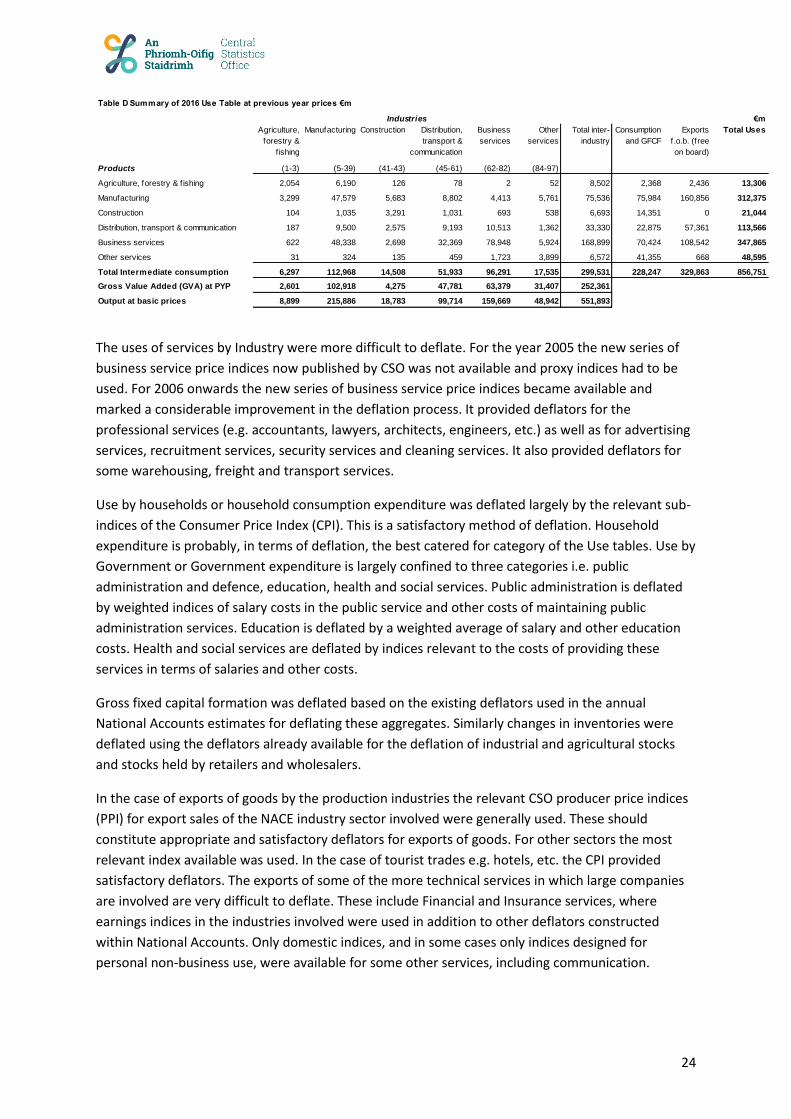
24
The uses of services by Industry were more difficult to deflate. For the year 2005 the new series of
business service price indices now published by CSO was not available and proxy indices had to be
used. For 2006 onwards the new series of business service price indices became available and
marked a considerable improvement in the deflation process. It provided deflators for the
professional services (e.g. accountants, lawyers, architects, engineers, etc.) as well as for advertising
services, recruitment services, security services and cleaning services. It also provided deflators for
some warehousing, freight and transport services.
Use by households or household consumption expenditure was deflated largely by the relevant sub-
indices of the Consumer Price Index (CPI). This is a satisfactory method of deflation. Household
expenditure is probably, in terms of deflation, the best catered for category of the Use tables. Use by
Government or Government expenditure is largely confined to three categories i.e. public
administration and defence, education, health and social services. Public administration is deflated
by weighted indices of salary costs in the public service and other costs of maintaining public
administration services. Education is deflated by a weighted average of salary and other education
costs. Health and social services are deflated by indices relevant to the costs of providing these
services in terms of salaries and other costs.
Gross fixed capital formation was deflated based on the existing deflators used in the annual
National Accounts estimates for deflating these aggregates. Similarly changes in inventories were
deflated using the deflators already available for the deflation of industrial and agricultural stocks
and stocks held by retailers and wholesalers.
In the case of exports of goods by the production industries the relevant CSO producer price indices
(PPI) for export sales of the NACE industry sector involved were generally used. These should
constitute appropriate and satisfactory deflators for exports of goods. For other sectors the most
relevant index available was used. In the case of tourist trades e.g. hotels, etc. the CPI provided
satisfactory deflators. The exports of some of the more technical services in which large companies
are involved are very difficult to deflate. These include Financial and Insurance services, where
earnings indices in the industries involved were used in addition to other deflators constructed
within National Accounts. Only domestic indices, and in some cases only indices designed for
personal non-business use, were available for some other services, including communication.
€m
Agriculture,
forestry &
f ishing
Manufacturing Construction Distribution,
transport &
communication
Business
services
Other
services
Total inter-
industry
Consumption
and GFCF
Exports
f.o.b. (free
on board)
Total Uses
Products (1-3) (5-39) (41-43) (45-61) (62-82) (84-97)
Agriculture, forestry & f ishing 2,054 6,190 126 78 2 52 8,502 2,368 2,436 13,306
Manufacturing 3,299 47,579 5,683 8,802 4,413 5,761 75,536 75,984 160,856 312,375
Construction 104 1,035 3,291 1,031 693 538 6,693 14,351 0 21,044
Distribution, transport & communication 187 9,500 2,575 9,193 10,513 1,362 33,330 22,875 57,361 113,566
Business services 622 48,338 2,698 32,369 78,948 5,924 168,899 70,424 108,542 347,865
Other services 31 324 135 459 1,723 3,899 6,572 41,355 668 48,595
Total Intermediate consumption 6,297 112,968 14,508 51,933 96,291 17,535 299,531 228,247 329,863 856,751
Gross Value Added (GVA) at PYP 2,601 102,918 4,275 47,781 63,379 31,407 252,361
Output at basic prices 8,899 215,886 18,783 99,714 159,669 48,942 551,893
Industries
Table D Summary of 2016 Use Table at previous year prices €m

25
Balancing of PYP tables
Supply and Use tables should balance. This is rarely achieved on the first compilation of the tables.
There is generally a discrepancy between Supply and Use when the tables are initially compiled.
Investigations are then carried out into the larger discrepancies and errors may be discovered or
improved sources may be found for some of the estimates which reduce the discrepancies. Finally a
mechanical procedure may be applied to balance one of the tables to agree with the other.
The initial exploratory Supply and Use tables in PYP almost balanced in the initial versions. In fact the
tables were so close to balancing that they were published without any specific adjustment applied
to achieve a perfect balance. The 2006 total Use in PYP exceeded total Supply by only 0.121% while
in 2007 Use exceeded Supply by 0.158%. The 2008/2009 Supply and Use PYP tables again were
almost balanced, though on this occasion were mechanically balanced. The 2012, 2013 and 2014
tables were both closely balanced, with a total difference of less than 0.03%, 0.04% and 0.12%
respectively. The degree of “automatic” balancing by product which was required to remove the
residual imbalances remaining at the end was small. The 2016 PYP tables were again closely
balanced between deflated Supply and deflated Use (0.69%). They were mechanically balanced and
adjusted to ensure aggregate and sub-aggregate consistency with the published national accounts,
though again the required intervention at an aggregate level was generally small.
The link between Supply and Use tables at current and constant prices
The link between Supply and Use tables at current prices and Supply and Use tables at constant
prices for two successive years is shown below.
• Supply and Use tables of year t at prices of year t-1 divided by the Supply and Use tables of
year t-1 at current prices of year t-1 yield the corresponding volume indices.
• Supply and Use tables at current prices of year t divided by the Supply and Use tables of year
t at prices of year t-1 yield the corresponding price indices.
• Finally, from the Supply and Use tables at current prices of year t and year t-1 the
corresponding value indices can be derived.
The tables with derived volume indices reflect the real growth rates for all sectors and products of
the economy. The tables with derived price indices present the “inflation” rates and the tables with
derived value indices show the nominal growth rates of transactions.

26
GVA Volume changes
The primary purpose of compiling Supply and Use tables at PYP is to derive volume changes in GDP
and its major constituent components from year to year. Ireland, like most other countries regularly
compiles volume estimates of GDP growth. These are published quarterly and annually.
In Ireland there are two methods used to derive these estimates (i.e. expenditure and output) and
they are averaged. The output method is generally compiled by projecting previous year weights by
volume indicators for industrial and services sectors. Examples of volume indicators are the CSO’s
monthly series of output change in manufacturing industry or passenger miles travelled in the
transport industry, etc. The expenditure method is derived by deflating the main final demand
aggregates by overall deflators and subtracting imports at PYP.
However the Supply and Use tables at PYP are regarded as providing a more definitive view of
volume changes. They provide a framework for double deflation (i.e. separate deflation of outputs
and inputs or of “Supply” and “Use”) in the production method. This is regarded as superior to
projecting forward the ‘value addeds’ (or Supply minus Use) by output indicators as the latter
method assumes no change in the ratios of inputs to outputs. The Supply and Use tables at PYP also
facilitates balancing of the expenditure method with the production method as an added advantage.
Values of the main National Accounts aggregates (e.g. GDP, PCE, Capital Formation, etc.) can be
compared in PYP terms with their counterparts in current terms from the NIE publication with which
they were aligned when compiling the S&UT tables (NIE 2018 in the case of the 2016 S&UT). These
comparisons provide estimates of “volume” changes or real growth over the year in the aggregates
concerned.
A detailed illustration of the PYP Tables are provided in the accompanying ‘Overview’ presentation.
27
Intermediate Tables The following describes the 2015 Input-Output Tables (published 2018).
Use Table at basic prices (Table 3 of 2015 publication)
Use Table for domestic inputs at basic prices (Table 4)
Use Table for imports at basic prices (Table 5)
Use Table for trade margins (Table 6)
Use Table for taxes less subsidies on products (Table 7)
These five tables are ‘intermediate’ tables. They are calculated using the Supply table and the Use
table. In turn they are used to create the Input-Output tables. The flow can be simplified as follows:
Balanced Supply & Use tables → Use tables at basic prices → Domestic & Imported Use tables →
Symmetric Input-Output tables → Coefficient table → Leontief table
The following describes the 2015 Intermediate Tables (published 2018)
These intermediate tables allow us to create the Input-Output tables. Supply is measured in basic
prices as we have seen, so we also need to recast the Use table (in purchasers’ price) to basic prices.
We have seen above that the supply at basic prices is transformed to purchasers’ prices by the
addition of margins and taxes less subsidies on products. Consequently we need to create a Use
table of each of these three columns in the Supply table. We then add/subtract these figures from
the Use table at purchasers’ prices to create a Use table at basic prices. Also we require a domestic
Input-Output table to create a set of domestic multipliers. Consequently we also need to
disaggregate the Use table into domestic inputs/uses and imported inputs/uses. Frequent analysis
and adjustments throughout the process of calculating these intermediate tables are required. For
example, use cannot be negative – on first run domestic inputs/uses (which are calculated as the
residual of total use minus imported use) can throw up negative cells. These need to be examined
and understood and adjustments made to ensure all cells are positive, while retaining column/row
consistency throughout.
Quick run through of intermediate tables’ calculation:
We begin with the 2015 Use table at purchasers’ prices (Table 2). We then create a Use table for
trade margins (Table 6). We can see that there is consistency between the trade margin column in
the Supply table (Table 1) and the total margin uses column in Table 6. For example NACE 1-3
product margin in Table 1 is €1,790 million in 2015. The sum of the NACE 1-3 product row in Table 6
is also €1,790 million, and so on for each product code.
How is the Use for trade margins table (Table 6) created?
We have NACE 45 (Motor trade), NACE 46 (Wholesale trade) and NACE 47 (Retail trade) margins.
These data are mainly sourced from the ASI (there are also CIP data used in NACE 46). A Use table is
created for each of these four elements. For NACE 45, the positive margin mostly sits in the NACE 29
(Motor vehicles) product row and the PCE column, with some in GFCF. For NACE 46, the margin is
distributed across most columns/products. For NACE 47 the margin is distributed across the PCE

28
column. In all cases the sum of each column, for each type of margin, is zero. The matching negative
margin sits in the NACE 45, NACE 46 and NACE 47 product rows respectively.
How is the Use table for product Taxes and subsidies (Table 7) created?
This table is composed of a separate product taxes use table and a product subsidies table. The
product taxes table in turn is composed of four separate tables – one each for product taxes home
production, excise on imports, customs on imports and VAT. A product subsidies use table is also
calculated. The sum of the tables is the net taxes use table.
We then subtract the trade margins (Table 6), subtract the product taxes and add the (negative)
subsidies (Table 7) to the Use table at purchasers’ prices (Table 2) to convert to the Use table at
basic prices (Table 3).
If we take the example of 2015 NACE 1-3 industry use of NACE 1-3 products. In the Use table at
purchasers’ prices (Table 2) this is €2.012 billion. We subtract the Table 6 figure of €230 million and
the Table 7 figure of €17 million to get the Table 3 figure of €1.765 billion (i.e. €2.012 billion - €230
million - €17 million = €1.765 billion).
Calculation of the Use table for domestic inputs at basic prices (Table 4) and the Use
table for imports at basic prices (Table 5)
Table 3 is the starting point. In the Supply table (Table 1) we have a product import column. We then
create a Use table of imports (Table 5) and subtract this from Table 3 to give us Table 4. We will use
the example of NACE 1-3 again. In the 2015 Supply table we see that the total imports of NACE 1-3
product were €1.261 billion. If we look at the right hand column of Table 5 we see that the total for
NACE 1-3 is again €1.261 billion, split across the different columns. For NACE 1-3 industry use of
NACE 1-3 product, Table 3 is €1.765 billion. Of this €254 million is imported (Table 5) meaning that
the domestic element is €1.511 billion (Table 4) (i.e. €1.765 billion - €254 million = €1.511 billion).
Repetition with the Supply & Use, intermediate and Input-Output tables
As we can see from the above, there is significant repetition/consistency required within and across
this full suite of tables. Given that the same products and/or industries are being examined, whether
the supply (output) or use (demand) is total, domestic or imported, then there will be significant
number of cells or sums of cells which will make a regular appearance. Let’s look at a few examples.
In the 2015 Supply table (Table 1) NACE 1-3 industry output was €8.530 billion. In the 2015 Use table
(Table 2) intermediate consumption was €6.080 billion while GVA was €2.450 billion. This means
that the implied output from the Use table is €8.530 billion, as per the Supply table output. Looking
at products, we see that both NACE 1-3 product supply and use was €9.112 billion. Domestic supply
of NACE 1-3 product from Table 1 was €7.277 billion, while Table 9 Domestic Input-Output table
NACE 1-3 inputs and outputs were also both €11.633 billion. Similarly total domestic supply and
imports of NACE 1-3 products from Table 1 were €9.717 billion, while this is repeated in the total
uses column in the right hand side of Table 8 (Total Input-Output table).
More details on the Intermediate tables and Repetition are provided in the accompanying
‘Overview’ presentation.

29
Input-Output Tables The following describes the 2015 Input-Output Tables (published 2018).
We will now move on to the creation of the symmetric Input-Output tables and their associated
Coefficient and Leontief tables.
Balanced Supply & Use tables → Use tables at basic prices → Domestic & Imported Use tables →
Symmetric Input-Output tables → Coefficient table → Leontief table
Symmetric Input-Output Table of total product flows (product by product) (Table 8)
Symmetric Input-Output Table for domestic output at basic prices (Table 9)
Symmetric Input-Output Table of imported product flows (product by product) (Table 10)
These tables are derived from the preceding intermediate tables. The transformation of the Supply
and Use tables to Input-Output tables is based on the commodity technology assumption2.
What does this mean?
It is important to understand that in converting the asymmetric use table to a symmetric format, a
number of assumptions are made with regard to the production of secondary production or by-
products of the production process – i.e. the off-diagonal elements shown in the domestic part of
the Supply Table. In producing such secondary products, we either assume that there will be no
difference in the structure of inputs required from that shown by the industry (an Industry
Technology Assumption), or, conversely, we can assume that in producing secondary outputs an
industry would need to use the inputs typically shown by the main industry producing the product in
question (a Product Technology Assumption)3. The domestic Input-Output table (Table 9) forms the
basis of Table 12 which contains the Leontief inverse coefficients which are required by users of
Input-Output techniques to assess the implications of changes in demand on the various sectors of
the economy. It purports to show the use made of domestically produced products in the
manufacture or provision of other products. Below is a summary of the domestic Input-Output table.
2015 Symmetric Input-Output Table of domestic product flows €m
2 See Handbook of Input-Output Table Compilation and Analysis, United Nations Publication, Sales No. E99XVII.9, New York, 1999 3 See also Chapter 11 of the Eurostat Manual of Supply, Use and Input-Output Tables for information
about transformation models. http://ec.europa.eu/eurostat/web/products-manuals-and-guidelines/-/KS-RA-07-013
Table C Summary of 2015 Symmetric Input-Output table of domestic product flows €m Products €m
Agriculture,
forestry &
fishing
Manufacturing Construction Distribution,
transport &
communication
Business
services
Other
services
Inter-
industry
Consumption
and GFCF
Exports
f.o.b. (free
on board)
Total
outputs
Products (1-3) (5-39) (41-43) (45-61) (62-82) (84-97)
Agriculture, forestry & fishing 1,575 3,906 97 40 3 30 5,652 1,193 1,611 8,456
Manufacturing 874 7,482 1,868 2,073 1,243 1,116 14,655 5,726 164,091 184,472
Construction 52 944 3,196 626 381 729 5,930 11,489 0 17,419
Distribution, transport & communication 212 3,466 403 4,614 3,235 1,142 13,072 27,514 51,212 91,798
Business services 199 3,005 1,281 8,485 27,392 3,414 43,777 28,015 99,424 171,215
Other services 41 256 116 585 1,724 4,124 6,846 40,488 792 48,126
Total Intermediate consumption 2,953 19,059 6,962 16,424 33,979 10,556 89,931 114,424 317,131 521,486
Imports 2,909 81,552 4,961 21,328 66,420 5,249 182,418 57,862 0 240,280
Product taxes less subsidies 176 646 251 1,390 2,220 859 5,542 13,329 0 18,871
Total at purchasers' prices 6,038 101,257 12,173 39,141 102,618 16,663 277,891 185,615 317,131 780,638
COE 638 10,431 2,929 18,077 20,337 25,238 77,649
GOS 3,353 72,035 2,288 33,984 47,429 6,181 165,270
Other taxes less subsidies -1,573 749 28 597 831 43 676
Value added 2,418 83,215 5,245 52,657 68,597 31,462 243,595
Total inputs (= total outputs) 8,456 184,472 17,419 91,798 171,215 48,126 521,486
30
The structure of the domestic Input-Output table (I-O table) is similar to the structure of the Use
table but differs in the following ways:
• The I-O table is product-by-product and thus shows the use of products in the production of
other products.
• Purchases are valued at basic prices. (The basic price is the price received by the producer
for a good or service produced minus any tax payable as a consequence of its production
plus any subsidy received as a consequence of its production. It excludes any trade margin. It
is therefore the price retained by the producer.)
• The I-O table is a domestic Input-Output table and thus shows the use made of domestically
produced products in the production of other products. Information on the imports of goods
and services for further production and for final consumption is provided in the imports row
followed by a row of product taxes less subsidies. Adding the product taxes less subsidies to
the values at basic prices converts the intermediate consumption to purchasers’ prices.
• The Input-Output table is symmetric. The sum of the entries in any row is equal to the sum
of the entries in the corresponding column. This is because total output of a product, shown
at the end of a row, can be analysed into various costs going into its production, shown
down the column. These column sums and row sums are equal to the total domestic supply
column of 2015 Table 1.
What are symmetric tables?
Supply and Use Tables can form a central part of the system of national accounts. These tables can
act as an integration framework for balancing the national accounts and determining a consistent
estimate of GDP. They can also constitute the basis from which macroeconomic models and impact
analysis can be derived in the form of symmetric input-output tables. Symmetric matrices present a
version of the Use table as either industry by industry or product by product, as opposed to the
standard (non-symmetrical) product by industry Use table.
To put this more simply, a symmetric Input-Output table can be considered a ‘blending’ of the
Supply table and the Use table into a single table. This allows for examination of inputs (columns)
and outputs (rows) simultaneously. Given that the table is symmetric, the sum of the column will
equal the sum of the rows (both individually and collectively).
Since the I-O models are generally used to model the impacts of changes on the domestic economy,
the first step in generating the symmetric tables is to extract the valuation and imports tables from
the combined (i.e. includes imported products) Use Table at purchasers’ price. This gives a Domestic
Use Table at basic prices. We have examined this table above. The Supply and Use Tables at basic
prices constitute the database which is required for the transformation to Input-Output tables.
Quick run through of Input-Output tables calculations:
31
These tables are the product of the preceding tables. The domestic I-O table can be expressed as the
following formula:
X_p = U*S^-1*q
Where:
U = Use table (domestic) at basic prices with imports and taxes shown in separate rows
S = Supply table (domestic produce part, with rows equal to vector q)
Q = nxn matrix with row totals of S on the diagonal
X_p = product-by-product Input-Output table
We will work through these elements in turn.
U is the domestic use (Table 4) which we have discussed above.
S is 2015 Table 1 discussed above.
Q is the row total of the Supply matrix brought together – i.e. for example in NACE 16 we have €914
million of domestic supply of the product, most of which, but not all, is produced by NACE 16
industry (€875 million). Consequently the Q table simply moves all row output on to the diagonal
from the off-diagonal cells to the NACE 16 column.
S^-1*q is calculated by using the MINVERSE function in excel (MINVERSE returns the inverse matrix
for the matrix stored in an array) of the domestic supply table (S above). We then apply the MMULT
excel function (MMULT returns the matrix product of two arrays – an array with the same number of
rows as array1 and the same number of columns as array2) to this calculated array and the q matrix
calculated above (i.e. with all products on the diagonal).
Finally, to create the domestic Input-Output table (Table 9) we again use the MMULT function, this
time on the S^-1*q matrix and the U matrix (Table 4), thus ‘blending’ the domestic supply and the
domestic use tables together in a product-by-product array.
The lower elements (the GVA components – i.e. COE, CFC, NOS, Taxes on production, subsidies on
production) just require the final MMULT application.
The total Input-Output table (Table 8) is slightly more complicated in that the imports column of the
Supply table also need to be incorporated into the calculations, but thereafter follow the same
pattern.
Adjustments are then made, both to ensure all figures are positive and also for balancing purposes
(the RAS method) and regarding ensuring that the sum of the domestic and imports Input-Output
tables is equal to the total Input-Output table.
More details on the Input-Output tables are provided in the accompanying ‘Overview’ presentation.

32
Multipliers Coefficients of domestic product flows (Table 11)
The Leontief inverse of domestic flows with multipliers for other inputs (Table 12)
If there is an increase in final demand for a particular product, we can assume that there will be an
increase in the output of that product as producers react to meet the increased demand. This is the
direct effect. There will also be an increase in demand for other products (i.e. the intermediate
consumption needed for the production of that product) and so on down the supply chain. This is
the indirect effect. Table 12 attempts to measure the complete direct and indirect impacts on the
economy resulting from the increase in demand for domestic output of a given product. The Leontief
inverse in (Table 12) is derived from the domestic Input-Output table. Multipliers in Table 12 are
Type I. Following describes the 2015 multiplier Tables (published 2018).
How are these Leontief Type I multipliers calculated?
Using the preceding tables we can calculate the formula:
L = (I – A )-1 Where:
L = Leontief inverse matrix
I = Identity matrix
A = Direct requirements matrix – each cell of the l*l matrix divided by its column total
Quick run through of Coefficient table to Leontief table calculation
The Leontief is based on the Coefficient table, which in turn is based on the domestic Input-Output
table. For NACE 1-3 product*product (Table 9) there is a figure of €1,575 million. Total output (at the
foot of the column) is €8,456 million. The corresponding figure in the coefficient table therefore is
0.186 (i.e. €1,575 million/€8,456 million). As the total inputs/outputs figure is used, the column sums
to 1.
I is the identity matrix. In practice, this simply means that where the column = the row then a 1 is
placed in the cell. This creates a diagonal of 1’s in the table. We then calculate I – A. So in the NACE
1-3 coefficient of 0.186 we calculated above, this will be 0.814 (i.e. 1 – 0.186). We then use the
MINVERSE function on the resulting array (MINVERSE returns the inverse matrix for the matrix
stored in an array) to get the output multipliers. Finally we apply the MMULT excel function (MMULT
returns the matrix product of two arrays – an array with the same number of rows as array1 and the
same number of columns as array2) to the lower elements of the table (the GVA components – i.e.
COE, CFC, NOS, Taxes on production, subsidies on production) to produce the direct and indirect
multipliers for other inputs.
What do these multipliers tell us and how can they be used?
The upper portion of the 2015 Table 12 can be interpreted as follows, using products of agriculture,
forestry and fishing as an example.
Each €1 of final demand for domestic output of products of agriculture, forestry and fishing requires:
€1.239 output of domestically produced agriculture, forestry and fishing;
33
€0.007 output of domestically produced mining and quarrying products;
€0.049 output of domestically produced food products; etc.
The column sums shown in the row after product 97 are called output multipliers. These show how
much direct and indirect output is required, across all domestic products per €1 final demand for the
products named at the top of the column. But considerable duplication of output is included in this
approach. For example, if an increase in the final demand of product A by €1, requires an increase of
90% of this amount of output of product B, then output of both products has been increased by
€1.90. Gross outputs rather than net value added of products are combined in this table to give the
column aggregates thereby giving rise to duplication of output. The duplication arises because
product B is an ingredient in product A and its cost is absorbed in the final value of A, rather than
added to the final value of A.
The lower portion of Table 12 shows the direct plus indirect effect on other inputs per €1 final
demand. In each column the sum of the coefficients of imports, taxes less subsidies, compensation
of employees, consumption of fixed capital and net operating surplus add to 1. They show, after all
the cycles of production are completed, how the additional unit of final demand was spread over
these categories. There is no duplication in these coefficients.
Within the 58 product groups in 2015, six have import multipliers of value 0.15 or less and all of
these come from the services sector. This implies that for €1 extra demand of home produced
products from these product groups, less than 15% is spent indirectly on imports. The remainder,
more than 85% of the €1, remains within the economy. The product groups with the lowest import
multipliers include:
0.109 for Recreation and sports activities (NACE 93)
0.077 for Legal and accounting services (NACE 69)
0.027 for Cultural, arts and gambling services (NACE 90-92)
0.132 for Education services (NACE 85)
Conversely, the highest import multipliers include the following:
0.845 for Head office and management consultancy (NACE 70)
0.835 for Computer consultancy, data processing (NACE 62-63)
0.589 for Manufacture of Pulp, paper products (NACE 17)
0.585 for Manufacture of Electrical equipment (NACE 27)
0.575 for Insurance, reinsurance and pension funding (NACE 65)
Of an extra €1 demand for these products, there is an import content of at least 50%. One may
observe that several of codes with higher import multipliers are for products of manufacturing
industries. These industries are often dominated in Ireland by large multinational enterprises.
The domestic constituents of final demand are compensation of employees; net operating surplus;
consumption of fixed capital; and taxes less subsidies. Multipliers for each of these are found in the
last rows of the Leontief table.

34
These multipliers may be used for comparisons between branches. But care should be taken in their
interpretation. For example, they take no account of outflows of profits and dividends from each
branch and are thus related more to gross domestic product than to gross national product. They
describe the effects of marginal increases in final demand and cannot strictly be applied to large
changes. They do, however, recognise the interdependence of the various sectors of the economy
and for this reason can be a useful tool in the area of impact analysis.
Are there other multipliers?
Above I mentioned Type I multipliers. There are also Type II multipliers.
What is the difference between the two types of multipliers?
In Table 12 of the 2015 publication, the figures in row 64 (i.e. the figure of 1.495 for NACE 1-3, 1.307
for NACE 5-9, etc.) are Type I multipliers. As we have seen above, these are multipliers which
measure both the direct and indirect effects of this increase in demand. As a result of the direct and
indirect effects the level of household income throughout the economy will increase as a result of
increased employment, etc. A proportion of this increased income will be re-spent on final goods
and services (positive feedback effect). Type II multipliers also include these induced effects of the
additional demand. The CSO do not produce Type II multipliers, which would entail a different
construction of the preceding Input-Output tables.
How might this be done?
If we take the example of Table 9, the figures below row 65 (the figure of €2,953m for NACE 1-3)
would, depending on the multiplier, move above the line and be incorporated within the relevant
column of the matrix. Consequently Type II multipliers would be greater than Type I multipliers. If
you would like some further information on Type I and Type II multipliers, I suggest you have a look
at the following website and associated links which describes Input-Output multipliers for Scotland,
including both Type I and Type II.
http://www.scotland.gov.uk/Topics/Statistics/Browse/Economy/Input-Output/Mulitipliers
Both Type I and Type II multipliers may be used for comparisons between branches. But as stated
above, care should be taken in their interpretation. For example, they take no account of outflows of
profits and dividends from each branch and are thus related more to gross domestic product than to
gross national product. They describe the effects of marginal increases in final demand and cannot
strictly be applied to large changes. Type II multipliers, by necessity, involve more estimation and
include more assumptions than Type I multipliers and are therefore more speculative estimates.
They do, however, along with Type I multipliers, recognise the interdependence of the various
sectors of the economy and for this reason can be a useful tool in the area of impact analysis.

35
List of abbreviations and acronyms
API = Agricultural Price Indices
ASI = Annual Services Inquiry
BOP = Balance Of Payments
Capform = Capital Formation
CIF = Cost carriage, Insurance and Freight
CIP = Census of Industrial Production
COE = Compensation of Employees
COICOP = Classification Of Individual (final) Consumption by Purpose (households)
CPI = Consumer Price Index
DES = Department of Education and Skills
DKM = DKM Economic Consultants Review of the Construction Industry and Outlook
DOH = Department of Health
EHECS = Earning, Hours and Employment Costs Survey
ESA = European System of Accounts
FDT = Food, Drink and Tobacco
FOB = Free on Board
GDP = Gross Domestic Product
GFCF = Gross Fixed Capital Formation
GNI = Gross National Income
GVA = Gross Value Added
GWPI = General Wholesale Price index
HSE = Health Service Executive
IIU = Inter Industry Use
NACE = 'Nomenclature générale des Activités économiques dans les Communautés Européennes'. Classification of Economic Activities within the European Communities
NATACC = National Accounts
NEC = Not Elsewhere Classified
NIE = National Income and Expenditure
NPISH = Non-Profit Institutions Serving Households
N/R = Not Relevant
PCE = Personal Consumption and Expenditure
PPI = Producer Price Index
PRODCOM = PRODuction COMMunautaire (Community Production)
RSI = Retail Sales Index
RM&I = Repair, maintenance and improvement
S&U = Supply and Use
SNA = System of National Accounts
SSPI = Services Producer Price Index
SUT = Supply and Use Tables
UV = Unit Value
VAT = Value Added Tax
WA = Weighted Average
WPI = Wholesale Price Index