Embed Size (px)
Citation preview
Supply Chain Intermediation When Retailers Lead*
Elodie AdidaSchool of Business Administration, University of California at Riverside, [email protected]
Nitin BakshiManagement Science and Operations, London Business School, [email protected]
Victor DeMiguelManagement Science and Operations, London Business School, [email protected]
To understand the joint impact of horizontal and vertical competition on supply chain intermediation,
we propose a model of competition in a three-tier supply chain where intermediaries compete to mediate
between competing retailers and capacity-constrained suppliers. We argue that in many important contexts
it is more realistic to model the retailers as Stackelberg leaders, and show that as a result intermediaries
should focus on products for which the supplier base (existing production capacity) is neither too narrow
nor too broad. We also find that the right balance of horizontal and vertical competition can entirely offset
double marginalization and lead to supply chain efficiency. Finally, on accounting for intermediaries’ private
information about the supply side, we find that surprisingly, competing retailers could potentially be better
off, relative to the case with complete information.
Key words : Supply chain, intermediation, vertical and horizontal competition, Stackelberg leader.
History : December 11, 2012
1. Introduction
The objective of this paper is to study the joint impact of horizontal and vertical competition
on supply chains with intermediation firms such as Li & Fung Limited, Global Sources, and The
Connor Group, which have enjoyed substantial success over the years. For instance, Li & Fung
Limited (herein L&F) doubled its revenue between 2004 and 2007 (Einhorn 2010), and its sales
almost tripled between 2002 and 2011 (The Telegraph 2012); see also Fung et al. [2008]. These
firms deal with many suppliers and offer intermediation services to numerous retailers (McFarlan
et al. 2007). When an intermediary receives an order from a retailer, it identifies from its supplier
*We are grateful for comments from Long Gao, Serguei Netessine, Guillaume Roels, Robert Swinney, Song (Alex)Yang, and seminar participants at the 2011 INFORMS Annual Meeting in Charlotte, the 2012 POMS Conference inChicago, the 2012 MSOM Conference in New York, the 2012 INFORMS Annual Meeting in Phoenix, the AndersonGraduate School of Management at UC Riverside, ESSEC Business School, the department of Management Scienceand Innovation at University College London, the Stuart School of Business at Illinois Institute of Technology, andSan Jose State University.

2 Adida, Bakshi, and DeMiguel: Supply chain intermediation
base the firms required to fulfill the order, and charges a margin to the retailer for its mediation.
For example, L&F acts as an intermediary between apparel suppliers across Asia and retailers such
as Walmart, Liz Claiborne, and Zara—see Cheng [2010] and Einhorn [2010].
Clearly, competition is a prominent aspect of supply chain intermediation, as described above.
However, the literature on intermediation, both in Economics and Operations, has essentially
focused on identifying rationales for the existence of intermediaries. We aim to address this gap
by improving our understanding of the joint impact of horizontal and vertical competition on
supply chain intermediation. To do so, we model a three-tier supply chain, where the middle tier
consists of a set of intermediaries who compete in quantities to mediate between the other two
tiers, which consist of quantity-competing retailers and capacity-constrained suppliers. A critical
difference from most existing models of multi-tier supply-chain competition is that our model
portrays the retailers as Stackelberg leaders with respect to the intermediaries. This is consistent
with the business model of firms such as L&F that orchestrate order-specific supply chains to
satisfy incidental demand from large retailers; see Knowledge@Wharton [2007].
We provide a complete analytical characterization of the symmetric supply chain equilibrium, and
use the closed-form expressions to answer three research questions. First, how does the competitive
environment affect the performance of retailers and intermediaries? Second, does the presence of
intermediaries necessarily lead to inefficiency in the supply chain? Third, can intermediaries exploit
their private information about the supply side to improve their bargaining position with respect
to the retailers?
With respect to the performance of intermediaries, we find that the intermediary profits are
unimodal with respect to the number of suppliers in its base. This is in direct contrast with the
insight from existing models of supply chain competition, in which suppliers lead. Based on that
literature, one might have expected that the larger the supplier base, the larger the market power of
the intermediaries and thus the larger their profits. This intuition does bear out when the size of the
supplier base is “small”. However, in a world where retailers lead, when the supplier base is “large
enough”, we show that the weakness of the suppliers becomes the weakness of the intermediaries,
and the retailers exploit their leadership position to increase their market power and retain greater
supply chain profits. A crucial implication of this result is that supply chain intermediaries should
focus on products for which the supplier base available is neither too narrow nor too broad; that is,
intermediaries should avoid specialty products as well as large-volume commodity products, and
focus on products in the middle range in terms of existing production capacity.
With respect to supply chain efficiency, we observe that the presence of intermediaries in the
supply chain does not necessarily result in inefficient supply chains; that is, the aggregate supply
chain profit in the decentralized chain with intermediaries is not necessarily smaller than that in
the centralized supply chain. The classic result on double marginalization would have suggested
otherwise (Spengler 1950). However, the differentiating feature of our analysis is that, along with
Adida, Bakshi, and DeMiguel: Supply chain intermediation 3
vertical competition, we simultaneously account for horizontal competition. It is well known that
the relative bargaining strength of players in a vertical relationship significantly determines the
extent of double marginalization. Further, increasing the number of within-tier competitors reduces
a specific player’s bargaining power in the vertical interaction. Such adjustments to competitive
intensity may be carried out at each tier. We find that there always exists an appropriate balance
between horizontal and vertical competition that completely offsets the effect of double marginal-
ization, and leads to supply chain efficiency.
Finally, we mentioned earlier that the retailers exploit their leadership position to increase their
market power with respect to the intermediaries. This leads one to wonder whether intermediaries
can exploit their private information about the supply side to extract greater rents. Indeed, it is
reasonable to assume that intermediaries will know the low-cost suppliers that they regularly deal
with better than retailers. We find that when intermediaries possess private information about
the supply sensitivity, its impact depends on the direction and extent of misperception in the
retailers’ belief about it. In particular, when the retailers underestimate the supply sensitivity, not
surprisingly the intermediary profits are lower than in the case with complete information because
the retailers believe that the supply sensitivity is smaller than it actually is and, as a result, they
offer a low price to the intermediary. However, the impact on the retailer profits is less obvious
because it depends on how much the retailers underestimate the supply sensitivity. When the
retailers grossly underestimate the sensitivity, their profits are smaller, but when the extent of
their misperception is moderate, the retailer profits are larger. The reason for this is that the
underestimation of supply sensitivity by the retailers has a dual effect on their profits: a negative
incomplete information effect, and a positive competition mitigation effect. The negative effect is
that the retailers believe the supply is less sensitive than it really is, and thus they offer a lower
than optimal (for retailers) price to the intermediary. The positive effect, however, is that the
missing information attenuates the intensity of competition among retailers—because the retailers
believe supply sensitivity is smaller than it actually is. Summarizing, when the retailers grossly
underestimate the supply sensitivity, the incomplete information effect dominates, and otherwise
the competition mitigation effect dominates.1
We make two contributions. First, we propose a model of supply chain intermediation (with
and without complete information) that incorporates both horizontal and vertical competition
and portrays the retailers as leaders. This representation is appropriate for the business model
of intermediary firms such as L&F. Second, we use this framework to shed new light on aspects
of supply chain intermediation such as intermediary product portfolios, supply chain efficiency,
and the impact of asymmetric information. In the process, we synthesize and extend two parallel
streams of literature: one on supply chain competition and the other on intermediation.
1 The results for the case when the retailers overestimate the supply sensitivity proceed along expected lines, and we
elaborate on them in Section 5.

4 Adida, Bakshi, and DeMiguel: Supply chain intermediation
The remainder of this manuscript is organized as follows. Section 2 discusses how our work relates
to the existing literature. Section 3 describes the three-tier model of supply chain competition.
Section 4 characterizes the equilibrium, discusses the properties of the equilibrium in terms of
intermediary performance and supply chain efficiency, and compares the equilibrium to those for
other models in the literature. Section 5 studies the effect of asymmetric information, and Section 6
concludes. Appendix A contains proofs for all results, Appendix B contains tables, Appendix C
contains figures, and a supplemental file gives Appendix D containing the analysis of the robustness
of our results to the use of a nonlinear marginal cost function.
2. Relation to the literature
2.1. Literature on supply chain competition
One of our contributions is to propose a model of multi-tier supply-chain competition in which
retailers lead. Most of the existing models of multi-tier supply-chain competition assume the retail-
ers are followers. A prominent example is Corbett and Karmarkar [2001], herein C&K, who consider
entry in a multi-tier supply chain with vertical competition across tiers and horizontal quantity-
competition within each tier. C&K assume the retailers face a deterministic linear demand function,
and they are followers with respect to the suppliers who face constant marginal costs.2 Portraying
retailers as followers is reasonable for many real-world supply chains (e.g., Dell, Coca-Cola, and
suppliers of luxury goods may well lead the supply chains for distribution of their products), but
may not be realistic in the context of supply chain intermediation firms like L&F. These firms
orchestrate demand-driven supply chains as a response to a specific order from a retailer facing
incidental demand; see Knowledge@Wharton [2007]. Chronologically, the retailer order precedes
the orchestration of the supply chain. Interestingly, we find that there is a fundamental difference
between the equilibrium for the model with retailers as followers (as in C&K) and the equilibrium
for our model with retailers as leaders: whereas C&K find that the profit of the intermediaries is
increasing in the number of suppliers, we find that the profit of the intermediaries is unimodal
in the number of suppliers. The unimodality of intermediary profits in the number of suppliers
results in the insight that intermediaries should avoid specialty as well as commodity products.
2 Several papers use variants of the multi-tier supply chain proposed by C&K with quantity competition at every tier
and where the retailers are followers: Carr and Karmarkar [2005] consider the case where there is assembly, Adida
and DeMiguel [2011] consider the case with multiple differentiated products and risk-averse retailers facing uncertain
demand, and Cho [2011] uses the framework by C&K to study the effect of horizontal mergers on consumer prices.
Even for two-tier supply chains, several papers consider models in which a single supplier leads several competing
retailers: Bernstein and Federgruen [2005] consider one manufacturer and multiple retailers who compete by choosing
their retail prices (they assume that the demand faced by each retailer is stochastic with a distribution that depends
on the retail prices of all retailers), Netessine and Zhang [2005] consider a supply chain with one manufacturer
and quantity-competing retailers who face an exogenously determined retail price and a stochastic demand whose
distribution depends on the order quantities of all retailers, Cachon and Lariviere [2005] consider one supplier who
leads competing retailers (their results hold both for the case where the retailers are competitive newsvendors and
when the retailers compete a la Cournot).

Adida, Bakshi, and DeMiguel: Supply chain intermediation 5
This insight seems to be in concordance with the type of products that command most of L&F
demand. These include apparel, toys and sporting goods (see Alberts [2010]), but not products
with ample production capacity such as agricultural commodities, or products with very limited
production capacity such as luxury goods and sophisticated electronic items.
Very few papers in the existing literature model the retailers as leaders. For example, Choi [1991]
considers a model in which one retailer leads two suppliers. His model assumes that the suppliers
possess complete information about the demand function facing the retailer, and that they exploit
this information strategically when making their production decisions. This assumption imposes
a level of sophistication on the suppliers’ strategic capabilities, and endows them with a degree
of information, that does not seem appropriate for the context of low-cost international suppliers
interacting with intermediaries such as L&F. Moreover, we show in Section 4.4 that the equilibrium
in Choi’s model with the retailer as leader is equivalent to that of the model by C&K, where
the retailers are followers, in the sense that the equilibrium quantity, retail price, and supply
chain aggregate profits are identical for both models. Overall, we think that assuming suppliers
can strategically exploit their complete knowledge of the retailers demand function, or for that
matter even strategically compete with numerous other similar suppliers, is not realistic in our
setting. This is crucial, because as we demonstrate in this paper, incorporating a more apt model
for suppliers, along with retailers leading the interaction, results in substantially different insights
than those suggested by the literature on supply chain competition.
Majumder and Srinivasan [2008], herein M&S, consider a model where any of the firms in a net-
work supply chain could be the leader, and study the effect of leadership on supply chain efficiency
as well as the effect of competition between network supply chains. Their model is closely related
to C&K’s, but the two models differ in three important aspects. First, while C&K consider a
serial multi-tier supply chain, M&S consider a network supply chain. Second, while C&K consider
both vertical competition across tiers and horizontal competition within tiers, M&S consider only
vertical competition within networks, and they consider horizontal competition only between net-
works. Third, while C&K assume constant marginal cost of manufacturing, M&S assume increasing
marginal cost of manufacturing, and they argue that, with wholesale price contracts, this is the
only assumption that results in equilibrium when suppliers follow.3
3 Perakis and Roels [2007] study efficiency in supply chains with price-only contracts, and consider a comprehensive
range of models, including both a push and a pull supply chain where the retailer leads. For the push chain (where
the retailer keeps the inventory) they assume that the retailer decides both the wholesale price and the quantity,
which results in the retailer keeping all the profits. In contrast, our model allows the intermediary to keep a positive
margin, as does L&F; see Fung et al. [2008]. Their pull supply chain does not capture the business model of firms such
as L&F since it requires inventory to be held by the intermediaries, something that is not observed in practice (Fung
et al. 2008). Another key difference between our model and the push and pull models by Perakis and Roels [2007] is
that they model horizontal competition in only a single tier, while we consider simultaneous horizontal competition
in multiple tiers of the supply chain.

6 Adida, Bakshi, and DeMiguel: Supply chain intermediation
Our model combines elements from the models of C&K and M&S and is tailored to the context
of supply chain intermediation. Similar to C&K we consider vertical and horizontal competition in
a multi-tier supply chain, but unlike C&K we model the retailers as leaders. As in M&S, we assume
increasing marginal costs of supply, but our motivation to do this, as we explain in §3.1.1, is not
only that this is the sole assumption that results in equilibrium for the case where retailers lead,
but also that this is realistic in the context of intermediary firms like L&F that use the existing
production capacity of their base of suppliers to satisfy incidental demand from retailers. Because
the suppliers use existing capacity, they do not have to make any additional capacity investments,
which are the main rationale for the existence of decreasing marginal costs of supply, and they are
likely to be subject to capacity constraints that will result in increasing marginal costs.
2.2. Literature on intermediation
Our work is related to the Economics literature on intermediation, which according to Wu [2004]
“studies the economic agents who coordinate and arbitrage transactions in between a group of
suppliers and customers.” One difference between our work and the work in this area is that
while the Economics literature has focused on justifying the existence of middlemen through their
ability to reduce fixed transaction costs (Rubinstein and Wolinsky [1987] and Biglaiser [1993]), we
focus on understanding the joint impact of horizontal and vertical competition on supply chain
intermediation and its operational aspects such as the quantity competition and supply chain
efficiency. Our modeling framework differs in several respects from the modeling frameworks used
in this literature. First, the intermediation literature generally models competition via bargaining,
whereas we assume quantity competition a la Cournot-Stackelberg. Second, the intermediation
literature generally assumes each buyer and seller is interested in a single unit and they each
have their own valuation, whereas we assume there is a consumer demand function and suppliers
and retailers are interested in multiple units. Finally, the Economics literature on intermediation
generally models the intermediaries as price-setting firms and focuses on characterizing the bid-
ask spread. In contrast, we simplify the price determination process by assuming a consumer
demand function and a Stackelberg framework, and track not only the intermediary margin but
also the overall efficiency of the supply chain. In summary, our model is closer to the multi-tier
competition models developed in the recent Operations Management literature, such as C&K, with
the difference that we model retailers as leaders, and our focus is on the operational aspects of
supply chain intermediation.4
Our work is also related to Belavina and Girotra [2011], who study intermediation in a supply
chain with two suppliers, one intermediary, and two buyers, with players in the same tier not
4 Although this is not the focus of our manuscript, it is easy to show that fixed transaction costs can also be used to
justify the existence of intermediaries within a supply chain competition context. Furthermore, in analysis available
from the authors upon request, we find that an operational rationale for the existence of intermediaries is that they
help diversify supply disruption risk.
Adida, Bakshi, and DeMiguel: Supply chain intermediation 7
competing directly. They provide a new rationale for the existence of intermediaries. Specifically,
they show that in a multi-period setting the intermediary is more effective in inducing efficient
decisions from the suppliers (e.g., quality related), because the intermediary has access to the
pooled demand of both buyers, and therefore superior ability to commit to future business with
each supplier. Again, a key difference between our work and theirs is that they focus on explaining
the existence of intermediaries, while we focus on understanding the joint impact of horizontal and
vertical competition on supply chain intermediation.
3. A model of multi-tier supply-chain competition where retailers lead
Modeling simultaneous horizontal and vertical competition in a multi-tier supply chain is a chal-
lenging problem. Fortunately, the seminal paper by C&K and the more recent paper by M&S have
led the way on this front and come up with a parsimonious framework to model supply chain com-
petition. We build on these well-established models and carefully justify any departure warranted
by our specific context of supply chain intermediation.
We consider a three-tier supply chain, where the first tier consists of a set of retailers who
compete in quantities to satisfy the consumer demand modeled by a deterministic linear demand
function. The retailers act as Stackelberg leaders with respect to the second tier consisting of a
set of intermediaries who compete in quantities to serve the retailers. The intermediaries act as
leaders with respect to a third tier consisting of a set of capacity-constrained suppliers.
As discussed in Section 2, we believe it is realistic to portray the retailers as leaders in the
context of intermediation firms such as L&F, which orchestrate demand-driven supply chains as a
response to a specific order from a retailer. For instance, the CEO and President of L&F, Bruce
Rockowitz describes their supply chains as being market-driven. Rather than selling what factories
make, their supply chains are matched to demand. He further points out that L&F orchestrates
supply chains on a customer-by-customer basis; that is, they assemble suppliers, manufacturers
and logistics service providers together and tailor a supply chain for each customer based on their
specific requirements (Knowledge@Wharton 2007). This sort of interaction is naturally captured
by a model in which retailers lead.
Our model is a static (one-shot) model of competition. Our motivation to focus on a static
game is that we study situations where a large retailer such as Walmart contacts an intermediary
firm such as L&F to satisfy incidental demand for certain new products (e.g., fashion apparel or
toys). Indeed, we believe large retailers are more likely to use intermediation services to satisfy
such incidental demand needs. For the case in which retailers such as Walmart are interested in
satisfying a recurrent demand for a specific item, they would be more likely to deal directly with the
suppliers rather than using the intermediation services. Moreover, as discussed above, in response
to the product request from the retailer, intermediaries orchestrate a one-time order-specific supply
chain.

8 Adida, Bakshi, and DeMiguel: Supply chain intermediation
Finally, we focus on wholesale price contracts between firms. We do so not only because there is
empirical support for their widespread usage and popularity (Lafontaine and Slade 2012), but also
because there is ample precedence in the supply chain literature (see, for instance, Lariviere and
Porteus [2001] and Perakis and Roels [2007]).5 An advantage of considering a static model with
wholesale price contracts is that these are standard assumptions in the literature on supply chain
competition (C&K, Choi 1991, M&S, Perakis and Roels 2007), and therefore a direct comparison
with that literature is possible. In the remainder of this section we give a detailed description of
our proposed model.
3.1. The suppliers
We consider S symmetric suppliers for a homogeneous product. Like M&S we assume that each
supplier has the following linearly increasing marginal cost function:
ps(q) = s1 + s2q, (1)
where s1 > 0 is the intercept, and s2 ≥ 0 is the sensitivity. The total cost of producing qs,j units is
thus increasing convex quadratic: c(qs,j) =∫ qs,j0
(s1 + s2q)dq= s1qs,j +(s2/2)q2s,j.
The profit of the jth supplier when supplying qs,j units at a price ps is simply the difference
between the revenue and the cost of producing qs,j units πs,j = psqs,j −s1qs,j − (s2/2)q2s,j. Moreover,
when the suppliers are offered a supply price ps by an intermediary, they optimally choose to
produce the quantity such that their marginal cost equals the supply price; that is, the quantity
qs,j such that ps = s1 + s2qs,j. This implies that the supplier profit can be rewritten as6
πs,j =s2q
2s,j
2. (2)
A few comments are in order. First, although we do not explicitly include the supplier capacity
constraints in our model, they are implicitly considered because in equilibrium a supplier would
never produce a quantity larger than (d1 − s1)/s2, where d1(> s1) is the intercept of the demand
function. Second, we assume that when the suppliers are faced with a price offer from an intermedi-
ary, they simply supply the quantity such that their marginal cost of supply equals the price offered
by the intermediary. This implies that our suppliers are not explicitly and strategically competing
with each other, but we believe this is an accurate representation of the decision process followed
by the type of low-cost suppliers that intermediary firms like L&F deal with.7 Third, although we
5 We have also considered a model where the retailers offer a two-part tariff to the intermediaries, but we find
that as the retailers set the contract terms to maximize their own profits while guaranteeing a reservation profit to
intermediaries, the intermediaries earn exactly their reservation profit, leaving all surplus to the retailers. Thus, this
is not adequate to model intermediation because we know that intermediaries do keep a margin.
6 An alternative model would involve a choice of ps that leaves the suppliers with zero profits. This does not strike
us as being realistic. Besides, the alternate formulation would not affect the qualitative nature of our insights.
7 The alternative would be to model suppliers as being cognizant of their strategic interaction with numerous other
suppliers and possessing knowledge of the retailers’ demand function. Neither of these assumptions seem very palatable
Adida, Bakshi, and DeMiguel: Supply chain intermediation 9
choose a linear marginal cost function for tractability and clarity of exposition, in Appendix D we
study the robustness of our results to the use of a nonlinear marginal opportunity cost function,
and we show that the insight that the intermediary profits are unimodal with respect to the num-
ber of suppliers holds also for a convex monomial marginal cost function. Finally, as we discuss
at the end of Section 3.1.1 and in Footnote 8, the assumption that suppliers are symmetric is not
fundamental to our analysis as all results can be derived from an aggregate marginal cost function.
3.1.1. On increasing marginal costs of supply. In addition to M&S, other authors who
have assumed increasing marginal costs include Anand and Mendelson [1997], Correa et al. [2011],
and Ha et al. [2011]. In particular, Ha et al. [2011] explain that this assumption: “is commonly used
in the inventory (Porteus 2002) and queuing (e.g., Kalai et al. [1992]) literatures. It is supported
by empirical evidence in industries such as petroleum refining (Griffin 1972) and auto making
(Mollick 2004)”.
M&S motivate their assumption of increasing marginal cost arguing that this assumption is
required to achieve an equilibrium when the suppliers are followers in the supply chain. Specifically,
[Majumder and Srinivasan 2008, p. 1190] claim: “ Since we have models in which the manufacturer
can be at the receiving end of a wholesale price contract, if she had a constant marginal cost, she
would choose to either not produce (if the wholesale price is lower than his marginal cost), produce
an arbitrarily large quantity (if the wholesale price is higher) or produce an indeterminate quantity
(if they are equal).”
While we agree with M&S that this is the only assumption that results in equilibrium, we also
believe this is the most realistic assumption in the context of supply chain intermediation, and
we give three different motivations for using this assumption. First, we focus on the case in which
intermediary firms such as Li & Fung use the existing production capacity of their network of
suppliers to satisfy incidental demand from retailers such as Walmart. Because the suppliers use
existing capacity, they do not make any additional capacity investments and thus they do not
incur any additional fixed costs. One of the key rationales for modeling decreasing marginal cost
of supply (economies of scale) is that any fixed cost of capacity investment can be defrayed over
multiple units. In the absence of incremental fixed costs, it is sufficient for the purposes of decision
making to capture the variable costs. In this setting, although marginal variable costs could be
constant for small quantities, they will inevitably increase as the order quantities approach the
capacity constraint of the suppliers. Citing a popular Economics textbook [Varian 1992, Section
5.2]: “When we are near to capacity, we need to use more than a proportional amount of the variable
inputs to increase output. Thus, the average variable cost function should eventually increase as
output increases.” Summarizing, we believe in the context of intermediaries using existing supplier
in our context. We also note that although we do not model explicit competition between suppliers, our model has the
appealing feature that as the number of suppliers increases, the resulting order allocation to each supplier decreases,
and therefore the marginal cost of supply decreases. This is qualitatively consistent with what one might expect if
the suppliers were competing.

10 Adida, Bakshi, and DeMiguel: Supply chain intermediation
capacity to meet retailers incidental demand, it is sufficient for decision making to consider only the
variable costs, and due to the capacity constraints, the associated marginal costs will be increasing
at least in the proximity of the capacity constraint.
Our second motivation for increasing marginal costs is to assume suppliers base their production
quantity decisions on their best outside option; that is, a supplier accepts a request to produce
one unit if the price offered by the retailer or intermediary is higher than the best outside offer
for that unit of capacity. For instance, assume a supplier has a capacity of 300 units and a unit
variable cost of 1 cent per unit. Assume also that the supplier has received two production offers
from other retailers or intermediaries. The first offer to produce 100 units at 10 cents per unit, and
the second to produce 100 units at 5 cents per unit. Then the supplier would accept a new offer to
produce 100 units at any price on or above its unit cost of 1 cent per unit, it would accept an offer
to produce 200 units provided the price offered was above 5 cents per unit, and would accept to
produce all 300 units if the price offered was above 10 cents. In other words, the supplier marginal
opportunity cost in cents per unit is the following increasing staircase function:
ps(q) =
1 if q≤ 100,
5 if 100< q≤ 200,
10 if 200< q≤ 300,
∞ if q > 300.
We believe that for the type of suppliers in Asia that intermediary firms such as L&F work with,
it is realistic to assume that the suppliers will make their production decisions based on how the
price offered by L&F compares to the offers from other clients.
Finally, the third motivation for increasing marginal costs is to relax the assumption that sup-
pliers are symmetric, and adopt an asymmetric aggregate view instead. Specifically, confronted
with a heterogeneous (in cost) supply base, the intermediaries would first order from the cheapest
supplier (up to its maximum capacity) and then would engage with progressively more expensive
suppliers. Such a supplier selection procedure would result in an increasing aggregate marginal
cost function (common to all intermediaries) that could be approximated with a linear function:
pS(Q) = s1 + s2 ∗Q with s2 > 0. As we argue below in Footnote 8, it is easy to see that the equi-
librium and the insights from our model would not change much if we used this aggregate supply
function.
3.2. The intermediaries
We consider I symmetric intermediaries. The lth intermediary chooses its order quantity qi,l to
maximize its profit; that is,
maxqi,l
[pi − ps
(qi,l +Qi,−l
S
)]qi,l,
where pi is the price offered by the retailer, Qi,−l is the total quantity ordered by the rest of the
intermediaries at equilibrium, and ps((qi,l+Qi,−l)/S) is the price that the intermediaries must pay
Adida, Bakshi, and DeMiguel: Supply chain intermediation 11
to acquire a total quantity qi,l +Qi,−l from the S suppliers.8 Note that here we are assuming that
the intermediaries are followers with respect to the retailers, but they are Stackelberg leaders with
respect to the suppliers. Moreover, from the definition of the supplier marginal cost function in
Equation (1), we can rewrite the intermediaries decision problem as
maxqi,l
[pi −
(s1 + s2
qi,l +Qi,−l
S
)]qi,l. (3)
3.3. The retailers
We consider R symmetric retailers. Similar to C&K, we assume retailers face a linear inverse
demand function9:
pr = d1 − d2Q. (4)
Then the kth retailer chooses its order quantity qr,k to maximize its profit anticipating the reaction
of the intermediaries; that is the retailer is a Stackelberg leader with respect to the intermediaries:
maxqr,k
[d1 − d2(qr,k +Qr,−k)− pi(qr,k +Qr,−k)] qr,k,
where the kth retailer as a Stackelberg leader anticipates the price pi(qr,k +Qr,−k) that it must
pay the intermediaries as a function of the total quantity Q= qr,k +Qr,−k, where Qr,−k is the total
quantity ordered by all retailers other than the kth retailer.
4. The equilibrium
In this section we characterize the supply chain equilibrium and analyze its properties. Section 4.1
gives closed-form expressions for the equilibrium quantities, Sections 4.2–4.3 give the interpretation
of these results, and Section 4.4 compares the equilibrium for our model to that for the models by
Corbett and Karmarkar [2001] and Choi [1991].
8 Note that given S suppliers, the aggregate supplier marginal opportunity cost function is pS(Q) = s1 + (s2/S)Q.
Moreover, the equilibrium can be determined from the aggregate supply function, and therefore the impact on the
equilibrium of an increase in the number of suppliers S is equivalent to the impact of a certain decrease in the supply
sensitivity s2, which is equivalent to an increase in the total production capacity in the supply chain. Finally, if we
were to consider a model based on an aggregate supply function pS(Q) = s1 + s2 ∗Q, as discussed at the end of
Section 3.1.1, the insights from our analysis would not change provided that s2 = s2/S.
9 Linear demand models have been widely used both in the Economics literature (see, for instance, Singh and Vives
[1984] and Hackner [2003]) as well as in the Operations Management literature (Goyal and Netessine [2007], Farahat
and Perakis [2011], and Farahat and Perakis [2009]). In addition to C&K, other authors have also used it in the
context of supply chain competition. Cachon and Lariviere [2005], for instance, mention that the results for their
model with competing retailers can be applied for the particular case of “Cournot competition with deterministic
linear demand”, and they give as an example a deterministic linear inverse demand function for a single homogeneous
product with retailer differentiation.

12 Adida, Bakshi, and DeMiguel: Supply chain intermediation
4.1. Closed-form expressions
Theorem 4.1 shows that the equilibrium quantities are as given in Table 1, Theorem 4.2 shows that
the monotonicity properties of the equilibrium quantities are as given in Table 3, and Theorem 4.4
gives the closed-form expression for the supply chain efficiency and characterizes its monotonicity
properties.
Theorem 4.1. Let d1 ≥ s1, then there exists a unique equilibrium for the symmetric supply chain,
the equilibrium is symmetric, and the equilibrium quantities are given by Table 1.
Theorem 4.2. Let d1 ≥ s1, the monotonicity properties of the equilibrium quantities are as stated
in Table 3. Moreover, the intermediary profit πi achieves a maximum with respect to the number
of suppliers for S = s2(I +1)/(d2I).
We now characterize the efficiency of the supply chain in the presence of intermediaries, defined
as the ratio of the aggregate supply chain profits in the decentralized and centralized supply chains.
The following proposition gives the optimal quantity and aggregate profit in the centralized supply
chain.
Proposition 4.3. The optimal production quantity and aggregate profit in the centralized supply
chain are Q= (d1 − s1)/(2d2 + s2/S) and πc = (d1 − s1)2/(2(2d2 + s2/S)).
The following proposition gives closed-form expressions of the supply chain efficiency, and char-
acterizes its monotonicity properties.
Theorem 4.4. The supply chain efficiency is
Efficiency =RI [s2R(I +2)+2(d2SI + s2(I +1))]
(d2SI + s2(I +1))2
2d2S+ s2(R+1)2
. (5)
Moreover the monotonicity properties of the efficiency with respect to the number of retailers,
intermediaries, and suppliers are as follows:
1. The efficiency is unimodal with respect to the number of suppliers S and reaches a maximum
equal to one for S = s2(R+ I +1)/(d2I(R− 1)) provided that R> 1. If R= 1, then the efficiency
is monotonically increasing in the number of suppliers, and tends to one as S →∞.
2. The efficiency is unimodal with respect to the number of intermediaries I and reaches a
maximum equal to one for I = s2(R + 1)/(d2S(R − 1) − s2) provided that d2S(R − 1) − s2 > 0.
Otherwise, the efficiency is monotonically increasing in the number of intermediaries, and tends to
R(2d2S+ s2)(2d2S+ s2(R+2))/((R+1)2(d2S+ s2)2) as I →∞.
3. The efficiency is unimodal with respect to the number of retailers R and reaches a maximum10
equal to one for R = (d2SI + s2(I + 1))/(d2SI − s2) provided that d2SI − s2 > 0. Otherwise, the
10 Note that the values of R,S and I respectively that maximize the efficiency may not be integers, in which case the
maximum would be reached at the integer value just below or above it. To keep the exposition simple, we approximate
the true integer maximum with the possibly non integer expressions above.
Adida, Bakshi, and DeMiguel: Supply chain intermediation 13
efficiency is monotonically increasing in the number of retailers, and tends to s2I(I + 2)(2d2S +
s2)/(d2SI + s2(I +1))2 as R→∞.
4.2. Monotonicity properties
Table 3 summarizes the monotonicity properties of the equilibrium quantities. The table gives sev-
eral intuitive results: (i) the total quantity produced in the supply chain is increasing in the number
of retailers, intermediaries, and suppliers, and decreasing in the demand and supply sensitivities,
(ii) the prices at each tier are decreasing in the number of players in following tiers, increasing in
the number of players in leading tiers, increasing in the supply function sensitivity, and decreasing
in the demand function sensitivity, and (iii) the retailer profits are increasing in the number of
intermediaries and suppliers, but decreasing in the number of retailers, and decreasing in both the
supply and demand sensitivities.
Compared to the above findings, the results about the intermediary profits are arguably more
interesting. Although expectedly the intermediary margin decreases in the number of intermediaries
and increases in the number of retailers, surprisingly the intermediary margin decreases in the
number of suppliers. Moreover, since the overall order quantity is monotonically increasing in the
number of suppliers, therefore the intermediary profits are unimodal with respect to the number of
suppliers, reaching their maximum for a finite number of suppliers. Based on the results in C&K
and Choi [1991], one might have expected that the larger the supplier base, the larger the market
power of the intermediaries and thus the larger their margin and profits. However, in a world where
retailers lead, when the supplier base is “large enough”, we show that the weakness of the suppliers
becomes the weakness of the intermediaries, and the retailers exploit their leadership position to
increase their market power and retain greater supply chain profits. Specifically, in the presence
of an infinite number of suppliers, the retailers know that the intermediaries can get an unlimited
quantity of the product at a price of s1 per unit. As a result, the retailers can exploit their leader
advantage to drive the intermediary price to the suppliers’ marginal cost s1. In this limiting case,
the retailers have all the market power and keep all profits. The crucial implication of this result is
that supply chain intermediaries should focus on products for which the supplier base available is
neither too narrow nor too broad; that is, intermediaries should avoid specialty products as well as
large-volume commodity products, and focus on products in the middle range in terms of available
production capacity.11
4.3. Efficiency
Theorem 4.4 gives the closed-form expression for the supply chain efficiency and characterizes its
monotonicity properties. Our main observation is that a supply chain efficiency equal to one (that
is, an efficient supply chain) can always be achieved in the presence of intermediaries provided there
11 Note that even though, as pointed out in the introduction, firms such as L&F deal with a large number of suppliers
across their portfolio; for any specific product, the relevant supplier base will be substantially smaller.
14 Adida, Bakshi, and DeMiguel: Supply chain intermediation
is the right balance of competition at the three tiers. To see this, note from Point 1 in Theorem 4.4
that provided the number of retailers is greater than one, we can always adjust the number of
suppliers so that efficiency one is achieved. Also, note that provided that there is a sufficiently large
number of suppliers and retailers, the condition d2S(R−1)−s2 > 0 will be satisfied, and thus from
Point 2 we have that there exists a number of intermediaries for which the supply chain efficiency
is equal to one. Finally, from Point 3 we see that provided there is a sufficiently large number of
suppliers and intermediaries we can always satisfy the condition d2SI − s2 > 0 and thus there will
exist a number of retailers for which the efficiency of the supply chain is equal to one.
The main takeaway from this analysis is that the presence of intermediaries in the supply chain
does not necessarily result in inefficient supply chains; that is, the aggregate supply chain profit in
the decentralized chain with intermediaries is not necessarily smaller than that in the centralized
supply chain. The classic result on double marginalization would have suggested otherwise (Spen-
gler 1950). However, accounting for competition in our model is the differentiating feature. It is
well known that the relative bargaining strength of players in a vertical relationship significantly
determines the extent of double marginalization. Further, increasing the number of within-tier
competitors reduces a specific player’s bargaining power in the vertical interaction. Such adjust-
ments to competitive intensity may be carried out at each tier. We find that there always exists an
appropriate balance between horizontal and vertical competition that completely offsets the effect
of double marginalization, and leads to supply chain efficiency.
4.4. Comparison to other models in the literature
We now give a detailed comparison of the equilibria for our proposed model and for the models
proposed by C&K and Choi [1991]. To do so, we first briefly state three-tier variants of the models
of C&K and Choi that are similar to our model, and then we compare the equilibria of the three
models.
As discussed in Section 2.1, our model also shares some common elements with that proposed
by M&S. Their model, however, does not consider horizontal competition within tiers, and instead
focuses on competition between supply networks. Moreover, M&S focus on how the equilibrium
depends on the position of the leader within the supply network, whereas we fix the leader position
to be at the retailer, which is the situation faced by the supply chain intermediary firms that we
are interested in. For these reasons, the equilibrium for M&S’s model is not comparable to that for
our model, and thus we focus in this section on the comparison with the equilibria for the models
by C&K and Choi, who consider serial multi-tier supply chain models with vertical and horizontal
competition similar to our model.
4.4.1. A Corbett-and-Karmarkar-type model. We first consider a three-tier version of
C&K’s model. The first tier consists of S suppliers who lead the second tier consisting of I inter-
mediaries who lead the third tier consisting of R retailers. There is quantity competition at all
Adida, Bakshi, and DeMiguel: Supply chain intermediation 15
three tiers. We focus on the case where only the first tier of suppliers face production costs, which
is the closest to our proposed model of intermediation.
The kth retailer chooses its order quantity qr,k to maximize its profit given an inverse demand
function pr = d1 − d2Q and for a given price requested by the intermediary pi:
maxqr,k
[d1 − d2(qr,k +Qr,−k)− pi)] qr,k.
The lth intermediary chooses its order quantity qi,l to maximize its profit for a given price
requested by the suppliers ps, and anticipating the price that the retailers are willing to pay for a
total quantity qi,l +Qi,−l:
maxqi,l
[pi (qi,l +Qi,−l)− ps] qi,l.
Finally, the jth supplier chooses its production quantity qs,j to maximize its profit anticipating
the price that the intermediaries are willing to pay for a total quantity qs,j +Qs,−j and given its
unit variable cost is s1:
maxqs,j
[ps (qs,j +Qs,−j)− s1] qs,j.
4.4.2. A Choi-type model. We now consider a three-tier version of Choi’s model with the
retailers as leaders. Choi assumes that suppliers know the demand function and exploit this knowl-
edge strategically when making production decisions. Moreover, Choi assumes that the suppliers
are margin takers with respect to the intermediaries. Thus the jth supplier’s decision problem is
maxqs,j
(d1 − d2 (qs,j +Qs,−j)−mr −mi − s1)qs,j,
where s1 is the unit production cost, and mr and mi are the retailer and intermediary margins,
respectively. Note that because pi =mr+mi+s1 it is apparent that the supplier’s decision problem
for the Choi-type model is exactly equivalent to the retailer’s decision problem for the C&K-type
model.
Following the spirit of Choi’s model with retailers as leaders, we assume that the intermediary
also knows the demand function and exploits this knowledge strategically when making order
quantity decisions. On the other hand, the intermediary is a follower with respect to the retailers
and thus is a margin taker with respect to the retailers, but the intermediary is a leader with
respect to the suppliers and thus anticipates the price requested by the suppliers to deliver a given
quantity. Therefore the lth intermediary decision can be written as
maxqi,l
(d1 − d2 (qi,l +Qi,−l)−mr − ps(qi,l +Qi,−l))qi,l.
Finally, the kth retailer in Choi’s model chooses its order quantity to maximize the profit given
the demand function and anticipating the price required by the intermediaries to supply a total
quantity qk,r +Qr,−k:
maxqk,r
(d1 − d2 (qk,r +Qr,−k)− pi(qk,r +Qr,−k))qk,r.
16 Adida, Bakshi, and DeMiguel: Supply chain intermediation
4.4.3. Comparing the C&K and Choi models. C&K give closed-form expressions for the
equilibrium quantities for their model. Choi also gives closed-form expressions for the equilibrium
quantities for his two-tier model with retailers as leaders, and it is straightforward to extend these
closed-form expressions for the three-tier variant of his model that we consider. The resulting
closed-form expressions are collected in the second and third columns of Table 2.
The striking realization when comparing the second and third columns in Table 2 is that the
equilibrium total order quantities in the C&K and Choi models coincide. Moreover, the aggregate
intermediary profits also coincide. Furthermore, a careful look at the expressions for the aggregate
profits of the retailers and suppliers reveals that the aggregate retailer profit in C&K’s model
coincides with the aggregate supplier profit in Choi’s model if one replaces the number of retailers
by the number of suppliers. Likewise, the aggregate supplier profit in C&K’s model coincides with
the aggregate retailer profit in Choi’s model if one replaces the number of suppliers by the number
of retailers. In other words, the equilibria of the C&K and Choi model are equivalent. We believe
the reason for this is the assumption in Choi’s model that the suppliers have perfect information
about the retailer demand function and exploit this strategically when making decisions. This is
not a realistic assumption for the intermediation context that we study.
4.4.4. Comparing our model to the C&K and Choi models. The most important
difference between the equilibrium to our model and those to the C&K and Choi models is in the
intermediary margins and profits. For all three models, the suppliers market power decreases in the
number of suppliers, and their profits become zero in the limit when there is an infinite number
of suppliers. The intermediaries’ margin and profit, however, behave quite differently for the three
models. In C&K’s model, the intermediaries’ margin increases with the number of suppliers; in
Choi’s model, it remains constant; and in our model, it decreases. As a result, for the C&K and Choi
models, the intermediary profits increase in the number of suppliers, because order quantities also
increase. In our model, on the other hand, the increase in the order quantities is not sufficient to
offset the decrease in margin and, as a result, the intermediary profits are unimodal in the number of
suppliers. The reason for this is that as the number of suppliers grows large, the retailers know that
intermediaries and suppliers will agree to produce at any price above s1, and therefore the retailers
can take advantage of their leading position to extract higher rents, leaving the intermediaries with
zero margin and profit for the limiting case where the number of suppliers is infinite.
Comparing the aggregate retailer profits in all three models, we observe that the equilibrium
retailer margins for our proposed model and the model by Choi are equal and they are both larger
than the equilibrium retailer margin for the model by C&K. Moreover, because the equilibrium
total quantity in the models by C&K and Choi are identical, this implies that the aggregate retailer
profit in the model by Choi is larger than that in the model by C&K. This is not surprising as

Adida, Bakshi, and DeMiguel: Supply chain intermediation 17
it is well known that a leading position often results in larger profits for a given player; see Vives
[1999].12
The question of whether the aggregate retailer profits are larger in our model than in those
by C&K and Choi is a bit harder to answer. Note that there is an additional parameter in our
model: the marginal cost sensitivity s2. This parameter enters the closed-form expression for the
equilibrium quantity in our model and thus it is difficult to compare to the other two models.
However, assuming the marginal cost sensitivity s2 equals the demand sensitivity d2, it is easy to
show that the equilibrium quantity in our model is larger than in the C&K and Choi models. This
implies that the equilibrium aggregate retailer profits in our model are larger not only than those
in the C&K model, but also than those in Choi’s model (for the case s2 = d2). Two comments are
in order. First, since in our proposed model the retailers act as leaders, they are able to capture
greater profits than in the model by C&K. Second, while Choi also captures the retailers as leaders,
he assumes that intermediaries and suppliers know the retailer demand function and exploit this
knowledge strategically. This assumption leaves the retailers in a weaker position compared to our
model.
We conclude that there are significant differences between the models by C&K and Choi [1991]
and our proposed model, particularly the leadership positions and information available within the
game, which result in different insights. Our model fits best situations when retailers act as leaders,
while C&K’s model is more appropriate when suppliers can be considered leaders. Choi’s model
makes sense when the retail demand function can realistically be known by all players.
5. The case with asymmetric information
An important insight from our analysis is that in a supply chain where retailers lead, they take
advantage of their leading position to increase their market power with respect to the intermedi-
aries. This leads one to wonder whether the intermediaries can exploit their private information
about the supply side to improve their bargaining position. Indeed, it is reasonable to assume that
the intermediaries have better knowledge of the supply sensitivity than the retailers, and that they
may strategically choose to exploit their knowledge. To answer this question, in this section we
study how the presence of asymmetric information about the supply sensitivity alters the balance
of market power between the retailers and the intermediaries.
5.1. The model and equilibrium
To model asymmetric information, we assume that retailers know the number of suppliers S and
the intercept s1 of the supplier marginal cost function, but they do not know whether the supply
12 Note that the retailer margin and profits in Choi’s model coincide with the supplier margin and profits in C&K’s
model after replacing the number of retailers with the number of suppliers, so as we argue above both models are
essentially equivalent.

18 Adida, Bakshi, and DeMiguel: Supply chain intermediation
sensitivity is high s2 = sH2 or low s2 = sL2 . Instead, we assume that all retailers share the prior belief
that there is a probability ν that the sensitivity is low (s2 = sL2 ) and 1−ν that it is high (s2 = sH2 ).
Like in the case with complete information, we assume the retailers act as Stackelberg leaders
with respect to the intermediaries. Specifically, the retailers offer a single price pi to intermediaries,
and they anticipate the intermediary best response (in terms of quantity) for each scenario (with
low or high sensitivity).13 As in the case with complete information, the intermediary best response
for each scenario is characterized by Theorem 4.1. Then the retailers maximize their expected profit
E[πr,k
]= ν
(d1 − d2(q
Lr,k +QL
r,−k)− pi)qLr,k +(1− ν)
(d1 − d2(q
Hr,k +QH
r,−k)− pi)qHr,k, (6)
where the first (second) term on the right-hand side of Equation (6) corresponds to the profit for
the case with low (high) sensitivity, qLr,k (qHr,k) is the kth retailer order quantity when the supply
sensitivity is low (high), which is determined by the intermediary best-response, and QLr,−k (QH
r,−k)
is the aggregate order quantity of all retailers except the kth retailer when the supply sensitivity
is low (high).
The presence of asymmetric information complicates the analysis substantially, so to keep the
exposition simple we restrict our analysis to symmetric equilibria. The following proposition gives
closed-form expressions for the unique symmetric equilibrium.
Proposition 5.1. Let d1 ≥ s1, then there exists a unique symmetric equilibrium for the supply
chain with asymmetric information. Moreover, for the case where the realized sensitivity is low
(s2 = sL2 ), the realized aggregate quantity (Q=QL) is
QL =RSI [(1− ν)sL2 + νsH2 ]
(1− ν)sL2 [d2SIsL2 /s
H2 +(I +1)sL2 ] + νsH2 [d2SI +(I +1)sL2 ]
d1 − s1R+1
and for the case where the realized sensitivity is high (s2 = sH2 ), the realized aggregate quantity
(Q=QH) is QH = (sL2 /sH2 )Q
L. Moreover, the rest of the realized equilibrium quantities are given
by the last column of Table 1 as a function of the realized aggregate quantity Q and the realized
supply sensitivity s2.
5.2. The impact of asymmetric information
The following proposition characterizes how the presence of asymmetric information affects the
equilibrium. To simplify the exposition we focus on the case when the ratio of the high to low
sensitivity (sH2 /sL2 ) is sufficiently large.14
13 This is the equivalent of a pooling contract in the standard treatment of games with asymmetric information.
Screening of the different types of intermediary is not possible in the context of wholesale price contracts because
only one contracting variable (price) is available. Note that we restrict our analysis to wholesale price contracts for
the reasons argued in Section 3.
14 See the proof in Appendix A for the exact threshold value. We have also analyzed the case where this ratio is small,
and the insights from the analysis are similar.
Adida, Bakshi, and DeMiguel: Supply chain intermediation 19
Proposition 5.2. Let d1 ≥ s1 and let sH2 /sL2 be sufficiently large, then the comparison between
equilibrium quantities in the supply chains with asymmetric and complete information is as indi-
cated in Table 4.
We now interpret the results in Table 4. We consider two cases: (i) the case where the true
(realized) sensitivity is low (s2 = sL2 ), and (ii) the case where the true (realized) sensitivity is high
(s2 = sH2 ). Another way to think about these two cases is to note that, for the case where the
realized sensitivity is low, the retailers’ prior belief overestimates the supply sensitivity, whereas
for the case where the realzied sensitivity is high, the retailers’ prior belief underestimates the
sensitivity.
When retailers overestimate the supply sensitivity, they are willing to offer a higher price to
the intermediaries compared to the case with complete information, which results in lower retailer
margin and profits, together with higher intermediary margin and profits. In other words, interme-
diaries facing low-sensitivity suppliers can exploit their superior knowledge of the supply sensitivity
to increase their profits at the expense of the retailers.
When retailers underestimate the supply sensitivity, on the other hand, they offer the intermedi-
aries a lower price compared to the case with complete information. This lower intermediary price
results in lower order quantities and lower intermediary profits. The retailer profits, however, could
be larger or smaller depending on their prior beliefs. Specifically, Table 4 shows that, when the
true (realized) sensitivity is high, the retailer profit is lower if it believes that the probability of
low sensitivity (ν) is greater than a certain threshold (ν0):
ν > ν0 ≡ α(R− 1)
α(R− 1)+ (sH2 /sL2 )(η−Rα)
,
where α= d2 + sH2 (I +1)/(SI) and η= d2sH2 /s
L2 + sH2 (I +1)/(SI).
For the case with a single retailer we have that ν0 = 0, and thus monopolist retailer profits are
always lower in the case with asymmetric information. Indeed, a monopolist retailer with perfect
information on supply sensitivity must be able to extract larger profits from the supply chain
than in the absence of perfect information, regardless of whether its prior belief overestimates or
underestimates the true supply sensitivity.
A more interesting result occurs when there are several competing retailers. For this case, when
retailers severely underestimate the supply sensitivity (ν > ν0), the retailer profits are smaller than
in the case with complete information. When the retailers moderately underestimate the supply
sensitivity (ν < ν0), their profits are larger in the presence of asymmetric information. The expla-
nation for this is that in the case in which multiple competing retailers underestimate the supply
sensitivity, the presence of asymmetric information has a negative and a positive effect on retailer
profits. The negative effect is that the retailers lack information about the supply sensitivity that
would help to identify the optimal price to offer to intermediaries. The positive effect, however,
is that this missing information attenuates the intensity of competition among retailers because

20 Adida, Bakshi, and DeMiguel: Supply chain intermediation
the retailers believe on average that supply sensitivity is smaller than it actually is and thus offer
a lower price to intermediaries. For the case where they severely underestimate the supply sensi-
tivity, the negative effect (incomplete information) dominates; for the case where they moderately
underestimate the sensitivity, the positive effect of asymmetric information (competition mitiga-
tion) dominates. This result is illustrated in Figure 1, which depicts the realized prices and profits
for the case where two retailers underestimate the supply sensitivity as a function of the retailers
belief probability ν.
One interesting implication of our analysis is that it is not always optimal for intermediaries to
keep their private information private. Specifically, when the retailers prior belief underestimates
the supply sensitivity, the intermediaries would benefit from disclosing their private information
to the retailers, if they can do this in a credible manner.
Finally, the following proposition shows that, although the insight that intermediary profits are
unimodal with respect to the number of suppliers is robust to the presence of asymmetric infor-
mation, the number of suppliers that maximizes intermediary profits in the case with asymmetric
information is larger (smaller) than in the case with complete information depending on whether
the retailers overestimate (underestimate) the supply sensitivity.
Proposition 5.3. Let d1 ≥ s1, then the intermediary profits in the presence of asymmetric infor-
mation are unimodal with respect to the number of suppliers, and the number of suppliers that
maximizes intermediary profits is larger (smaller) in the presence of asymmetric information for
the case with s2 = sL2 (s2 = sH2 ).
The main insight from Proposition 5.3 is that the presence of asymmetric information can result
in alterations to the intermediaries’ preferred product portfolio. When the retailers overestimate
(underestimate) the supply sensitivity, the preferred product portfolio is biased towards products
with more (less) available production capacity.
6. Conclusion
To understand the impact of horizontal and vertical competition on supply chain intermediation,
we study a model of supply chain competition with retailers as leaders. This is an appropriate repre-
sentation for the business model of successful sourcing companies such as L&F, Global Sources, and
The Connor Group. Our focus on the role of competition distinguishes our work from the bulk of
the prior literature on intermediation, which provides rationales for the existence of intermediaries.
Our analysis predicts that intermediaries prefer products with moderate levels of available capac-
ity on the supply side, which is consistent with the observation that L&F typically deals with
products such as apparel and toys, as opposed to large-volume commodities (e.g., agricultural
produce) or specialty items (e.g., luxury goods).
A key strategy espoused by L&F over the years has been to acquire other sourcing companies
such as Inchcape, Swire & Maclaine, and Camberley Enterprises (Fung Group 2012), with recent
speculation about further acquisitions (Reuters 2012). A natural question then is what the impact

Adida, Bakshi, and DeMiguel: Supply chain intermediation 21
of these acquisitions is not only on L&F, but also on the efficiency of the entire supply chain. Our
competition model provides a framework to think about these issues. Specifically, we find that
intermediation is not necessarily detrimental to supply chain performance, but rather that the
right balance of horizontal and vertical competition can entirely offset the adverse effect of double
marginalization.
Finally, we study the impact of asymmetric information in the context of supply chain inter-
mediation, and find that surprisingly intermediaries’ private information about supply sensitivity
may indirectly benefit retailers by alleviating inter-retailer competition.
Appendix A: Proofs for the results in the paper
Proof of Theorem 4.1.We prove the result in three steps. First, we characterize the best response
of the intermediaries to the retailers. Second, we characterize the retailer equilibrium as leaders
with respect to the intermediaries. Third, simple substitution into the best response functions leads
to the closed form expressions.
Step 1. The intermediary best response. We first show that the intermediary equilibrium
best response exists, is unique, and symmetric. It is easy to see from equation (3) that the interme-
diary decision problem is a strictly concave problem that can be equivalently rewritten as a linear
complementarity problem (LCP); see Cottle et al. [2009] for an introduction to complementarity
problems. Hence, the intermediary order vector qi = (qi,1, . . . , qi,I) is an intermediary equilibrium
if and only if it solves the following LCP, which is obtained by concatenating the LCPs charac-
terizing the best response of the I intermediaries 0≤ (−pi + s1)e+ (s2/S)Miqi ⊥ qi ≥ 0, where e
is the I-dimensional vector of ones, and Mi ∈RI ×RI is a positive definite matrix whose diagonal
elements are all equal to one and its off-diagonal elements are all equal to two. Thus this LCP
has a unique solution which is the unique intermediary equilibrium best response. Because the
intermediary equilibrium is unique and the game is symmetric with respect to all intermediaries,
the intermediary equilibrium must be symmetric. Indeed, if the equilibrium was not symmetric,
because the game is symmetric with respect to all intermediaries, it would be possible to permute
the strategies among intermediaries and obtain a different equilibrium, hereby contradicting the
uniqueness of the equilibrium.
We now characterize the intermediary equilibrium best response. To avoid the trivial case where
the quantity produced equals zero, we assume the equilibrium production quantity is nonzero. In
this case, for the symmetric equilibrium, the first-order optimality conditions for the intermediary
are: pi − (s1 + s2Q/S) − s2Q/(SI) = 0, where Q is the aggregate intermediary order quantity,
aggregated over all intermediaries. Hence, the intermediary price can be written at equilibrium as
pi = s1 + s2I +1
SIQ. (7)
Note that the intermediary margin is therefore mi = pi − ps = s2Q/(SI), and the intermediary
profit is
πi =mi
Q
I=
s2Q2
SI2. (8)
22 Adida, Bakshi, and DeMiguel: Supply chain intermediation
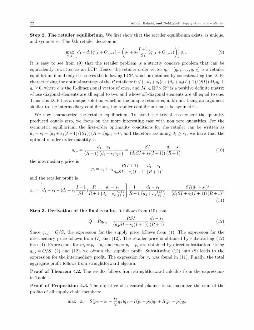
Step 2. The retailer equilibrium. We first show that the retailer equilibrium exists, is unique,
and symmetric. The kth retailer decision is
maxqr,k
[d1 − d2(qr,k +Qr,−k)−
(s1 + s2
I +1
SI(qr,k +Qr,−k)
)]qr,k. (9)
It is easy to see from (9) that the retailer problem is a strictly concave problem that can be
equivalently rewritten as an LCP. Hence, the retailer order vector qr = (qr,1, . . . , qr,R) is a retailer
equilibrium if and only if it solves the following LCP, which is obtained by concatenating the LCPs
characterizing the optimal strategy of theR retailers: 0≤ (−d1+s1)e+(d2 + s2(I +1)/(SI))Mrqr ⊥qr ≥ 0, where e is the R-dimensional vector of ones, and Mr ∈RR×RR is a positive definite matrix
whose diagonal elements are all equal to two and whose off-diagonal elements are all equal to one.
Thus this LCP has a unique solution which is the unique retailer equilibrium. Using an argument
similar to the intermediary equilibrium, the retailer equilibrium must be symmetric.
We now characterize the retailer equilibrium. To avoid the trivial case where the quantity
produced equals zero, we focus on the more interesting case with non zero quantities. For the
symmetric equilibrium, the first-order optimality conditions for the retailer can be written as
d1 − s1 − (d2 + s2(I +1)/(SI)) (R+ 1)qr,k = 0, and therefore assuming d1 ≥ s1, we have that the
optimal retailer order quantity is
qr,k =d1 − s1
(R+1)(d2 + s2
I+1SI
) =SI
(d2SI + s2(I +1))
d1 − s1(R+1)
, (10)
the intermediary price is
pi = s1 + s2R(I +1)
d2SI + s2(I +1)
d1 − s1(R+1)
,
and the retailer profit is
πr =
[d1 − s1 − (d2 + s2
I +1
SI)
R
R+1
d1 − s1(d2 + s2
I+1SI
)]
1
R+1
d1 − s1(d2 + s2
I+1SI
) =SI(d1 − s1)
2
(d2SI + s2(I +1)) (R+1)2.
(11)
Step 3. Derivation of the final results. It follows from (10) that
Q=Rqr,k =RSI
(d2SI + s2(I +1))
d1 − s1(R+1)
. (12)
Since qs,j = Q/S, the expression for the supply price follows from (1). The expression for the
intermediary price follows from (7) and (12). The retailer price is obtained by substituting (12)
into (4). Expressions for mi = pi − ps and mr = pr − pi are obtained by direct substitution. Using
qs,j = Q/S, (2) and (12), we obtain the supplier profit. Substituting (12) into (8) leads to the
expression for the intermediary profit. The expression for πr was found in (11). Finally, the total
aggregate profit follows from straightforward algebra.
Proof of Theorem 4.2. The results follows from straightforward calculus from the expressions
in Table 1.
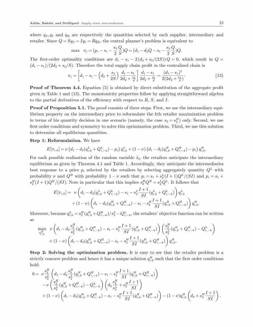
Proof of Proposition 4.3. The objective of a central planner is to maximize the sum of the
profits of all supply chain members:
max πc = S(pS − s1 − s22qS)qS + I(pi − pS)qI +R(pr − pi)qR
Adida, Bakshi, and DeMiguel: Supply chain intermediation 23
where qS, qI and qR are respectively the quantities selected by each supplier, intermediary and
retailer. Since Q= SqS = IqI =RqR, the central planner’s problem is equivalent to
max πc = (pr − s1 − s22
Q
S)Q= (d1 − d2Q− s1 − s2
2
Q
S)Q.
The first-order optimality conditions are d1 − s1 − 2 (d2 + s2/(2S))Q = 0, which result in Q =
(d1 − s1)/(2d2 + s2/S). Therefore the total supply chain profit in the centralized chain is
πc =
[d1 − s1 −
(d2 +
s22S
) d1 − s12d2 +
s2S
]d1 − s12d2 +
s2S
=(d1 − s1)
2
2(2d2 +s2S). (13)
Proof of Theorem 4.4. Equation (5) is obtained by direct substitution of the aggregate profit
given in Table 1 and (13). The monotonicity properties follow by applying straightforward algebra
to the partial derivatives of the efficiency with respect to R, S, and I.
Proof of Proposition 5.1. The proof consists of three steps. First, we use the intermediary equi-
librium property on the intermediary price to reformulate the kth retailer maximization problem
in terms of his quantity decision in one scenario (namely, the case s2 = sH2 ) only. Second, we use
first order conditions and symmetry to solve this optimization problem. Third, we use this solution
to determine all equilibrium quantities.
Step 1: Reformulation. We have
E[πr,k] = ν(d1 − d2(q
Lr,k +QL
r,−k)− pi)qLr,k +(1− ν)
(d1 − d2(q
Hr,k +QH
r,−k)− pi)qHr,k.
For each possible realization of the random variable s2, the retailers anticipate the intermediary
equilibrium as given by Theorem 4.1 and Table 1. Accordingly, they anticipate the intermediaries
best response to a price pi selected by the retailers by selecting aggregately quantity QL with
probability ν and QH with probability 1− ν such that pi = s1 + sL2 (I + 1)QL/(SI) and pi = s1 +
sH2 (I +1)QH/(SI). Note in particular that this implies sH2 QH = sL2Q
L. It follows that
E[πr,k] = ν
(d1 − d2(q
Lr,k +QL
r,−k)− s1 − sL2I +1
SI(qLr,k +QL
r,−k)
)qLr,k
+(1− ν)
(d1 − d2(q
Hr,k +QH
r,−k)− s1 − sH2I +1
SI(qHr,k +QH
r,−k)
)qHr,k.
Moreover, because qLr,k = sH2 (qHr,k+QH
r,−k)/sL2 −QL
r,−k, the retailers’ objective function can be written
as
maxqHr,k
ν
(d1 − d2
sH2sL2
(qHr,k +QHr,−k)− s1 − sH2
I +1
SI(qHr,k +QH
r,−k)
)(sH2sL2
(qHr,k +QHr,−k)−QL
r,−k
)
+(1− ν)
(d1 − d2(q
Hr,k +QH
r,−k)− s1 − sH2I +1
SI(qHr,k +QH
r,−k)
)qHr,k.
Step 2: Solving the optimization problem. It is easy to see that the retailer problem is a
strictly concave problem and hence it has a unique solution qHr,k such that the first order conditions
hold:
0 = νsH2sL2
(d1 − d2
sH2sL2
(qHr,k +QHr,−k)− s1 − sH2
I +1
SI(qHr,k +QH
r,−k)
)
− ν
(sH2sL2
(qHr,k +QHr,−k)−QL
r,−k
)(d2
sH2sL2
+ sH2I +1
SI
)
+(1− ν)
(d1 − d2(q
Hr,k +QH
r,−k)− s1 − sH2I +1
SI(qHr,k +QH
r,−k)
)− (1− ν)qHr,k
(d2 + sH2
I +1
SI
).

24 Adida, Bakshi, and DeMiguel: Supply chain intermediation
Using symmetry and the relation sL2QL = sH2 Q
H , which implies that at equilibrium QLr,−k =
(sH2 /sL2 )(R− 1)qHr,k, the first order conditions can be rewritten as
νsH2sL2
(d1 − s1 −
(d2
sH2sL2
+I +1
SIsH2
)(R+1)qHr,k
)+(1− ν)(d1− s1−
(d2 +
I +1
SIsH2
)(R+1)qHr,k = 0,
which results in
QH =R
R+1(d1 − s1)
1− ν+ νsH2sL2
νsH2sL2
(d2
sH2sL2
+ I+1SI
sH2
)+(1− ν)
(d2 +
I+1SI
sH2) .
Step 3: Determination of equilibrium quantities. It follows that
QL =R
R+1(d1 − s1)
ν+(1− ν)sL2sH2
(1− ν)sL2sH2
(d2
sL2sH2
+ I+1SI
sL2
)+ ν(d2 +
I+1SI
sL2 ).
The expressions for pi, ps, pr, mr, mi, πs, πi and πr follow similarly to the symmetric information
case by using the realized price sensitivity (sL2 or sH2 ) and realized cumulative quantity (QL or QH).
Proof of Proposition 5.2. In this proof, for each quantity in the table, we determine the sign of
the difference between the symmetric and asymmetric cases. Let QL,a be the aggregate quantity
produced with asymmetric information and QL,s the aggregate quantity produced with symmetric
information when s2 = sL2 . We have
QL,a −QL,s =R(d1 − s1)
R+1
ν+(1− ν)
sL2sH2
(1− ν)sL2sH2
(d2
sL2sH2
+ I+1SI
sL2
)+ ν(d2 +
I+1SI
sL2 )− 1
d2 + sk2I+1SI
=R(d1 − s1)
R+1
(1− ν)sL2sH2
d2
(1− sL2
sH2
)((1− ν)
sL2sH2
(d2
sL2sH2
+ I+1SI
sL2
)+ ν(d2 +
I+1SI
sL2 ))(
d2 + sL2I+1SI
) ,
and because sL2 < sH2 , it follows that QL,a −QL,s > 0. After substituting sH2 for sL2 and 1− ν for ν
and vice-versa, we obtain
QH,a −QH,s =R(d1 − s1)
R+1
νsH2sL2
d2
(1− sH2
sL2
)(ν
sH2sL2
(d2
sH2sL2
+ I+1SI
sH2
)+(1− ν)(d2 +
I+1SI
sH2 ))(
d2 + sH2I+1SI
) ,
thus QH,a −QH,s > 0.
The comparisons for ps, pr, pi, mi, πs and πi follow from the aggregate quantity comparison and
Table 1.
Let mL,ar be the retailer margin with asymmetric information and mL,s
r the retailer margin with
symmetric information when s2 = sL2 . We have
mL,ar −mL,s
r = d1 − s1 −(d2 + sL2
I +1
SI
)d1 − s1R+1
Rν+(1− ν)
sL2sH2
(1− ν)sL2sH2
(d2
sL2sH2
+ I+1SI
sL2
)+ ν(d2 +
I+1SI
sL2 )− d1 − s1
R+1
=d1 − s1R+1
R(1− ν)sL2sH2
d2
(sL2sH2
− 1)
(1− ν)sL2sH2
(d2
sL2sH2
+ I+1SI
sL2
)+ ν(d2 +
I+1SI
sL2 ),

Adida, Bakshi, and DeMiguel: Supply chain intermediation 25
and thus mL,ar <mL,s
r . Similarly, we obtain
mH,ar −mH,s
r =d1 − s1R+1
RνsH2sL2
d2
(sH2sL2
− 1)
νsH2sL2
(d2
sH2sL2
+ I+1SI
sH2
)+(1− ν)(d2 +
I+1SI
sH2 ),
and therefore mH,ar >mH,s
r .
Let πL,ar be the retailer profit with asymmetric information and πL,s
r the retailer profit with
symmetric information when s2 = sL2 . To ease exposition, let us denote γ = ν + (1 − ν)sL2 /sH2 ,
δ= sL2 /sH2 , α= d2 + sL2 (I +1)/(SI) and η= d2δ+ sL2 (I +1)/(SI). We have
πL,sr −πL,a
r =
(d1 − s1R+1
)21
α− γ
(1− ν)δη+ να
d1 − s1R+1
(d1 − s1 −α
γ
(1− ν)δη+ να
R(d1 − s1)
R+1
)
=
(d1 − s1R+1
)2
δ(1− ν)(α− η)(1− ν)δ(αR− η)+αν(R− 1)
α((1− ν)δη+ να)2,
after simplification. Note that α> η and therefore αR− η > 0 and it follows that πL,sr >πL,a
r .
For the case s2 = sH2 , it suffices to substitute sH2 for sL2 and 1− ν for ν and vice-versa, so we
redefine γ = (1− ν) + νsH2 /sL2 , δ = sH2 /s
L2 , α = d2 + sH2 (I + 1)/(SI) and η = d2δ + sH2 (I + 1)/(SI)
and we obtain
πH,sr −πH,a
r =
(d1 − s1R+1
)2
δν(α− η)νδ(αR− η)+α(1− ν)(R− 1)
α(νδη+(1− ν)α)2.
Note that now α< η and so we want to determine the sign of
∆πHr =−νδ(αR− η)−α(1− ν)(R− 1)
= ν(−δ(αR− η)+α(R− 1))−α(R− 1).
Because α< η, the sign of αR−η (and thus of ∆πHr ) varies depending on the input parameters. In
the case when the ratio δ= sH2 /sL2 is sufficiently large, then αR−η < 0. This occurs for sH2 /s
L2 > δ0,
where δ0 =R+ sH2 (I +1)(R− 1)/(d2SI). In this case, −δ(αR− η)+α(R− 1)> 0 and so ∆πHr < 0
when ν < ν0, and ∆πHr > 0 when ν > ν0, where
ν0 =α(R− 1)
−δ(αR− η)+α(R− 1)(∈ [0,1]).
Notice that if the ratio sH2 /sL2 is below the threshold δ0, then αR− η ≥ 0, ∆πH
r ≤ 0 and so πH,sr −
πH,ar ≤ 0 for all values of ν ∈ [0,1].
Proof of Proposition 5.3. If s2 = sL2 , the actual intermediary profit can be written as
πi =R2(d1 − s1)
2sL2SI2(R+1)2
(ν+(1− ν)δ
(1− ν)δ(d2δ+I+1SI
sL2 )+ ν(d2 +I+1SI
sL2 )
)2
,
where δ = sL2 /sH2 . It is easy to find that the derivative of the intermediary profit is, after simplifi-
cations,
∂πi
∂S=
R2(d1 − s1)2sL2
S2I2(R+1)2
(ν+(1− ν)δ
(1− ν)δ(d2δ+I+1SI
sL2 )+ ν(d2 +I+1SI
sL2 )
)2
×(−1+
2sL2 (I +1)
SI
ν+(1− ν)δ
(1− ν)δ(d2δ+I+1SI
sL2 )+ ν(d2 +I+1SI
sL2 )
).

26 Adida, Bakshi, and DeMiguel: Supply chain intermediation
It is clear that the intermediary profit is unimodal and reaches its maximum at (after simplifica-
tions)
SL =sL2 (I +1)
d2I
ν+(1− ν)δ
ν+(1− ν)δ2.
The result follows from the fact that for the case with symmetric information, Theorem 4.2 shows
that the intermediary profits are maximized for S = s2(I +1)/(d2I) and δ= sL2 /sH2 < 1.
The case when s2 = sH2 follows similarly after substituting sH2 for sL2 and ν for 1− ν (and vice-
versa).
Appendix B: Tables
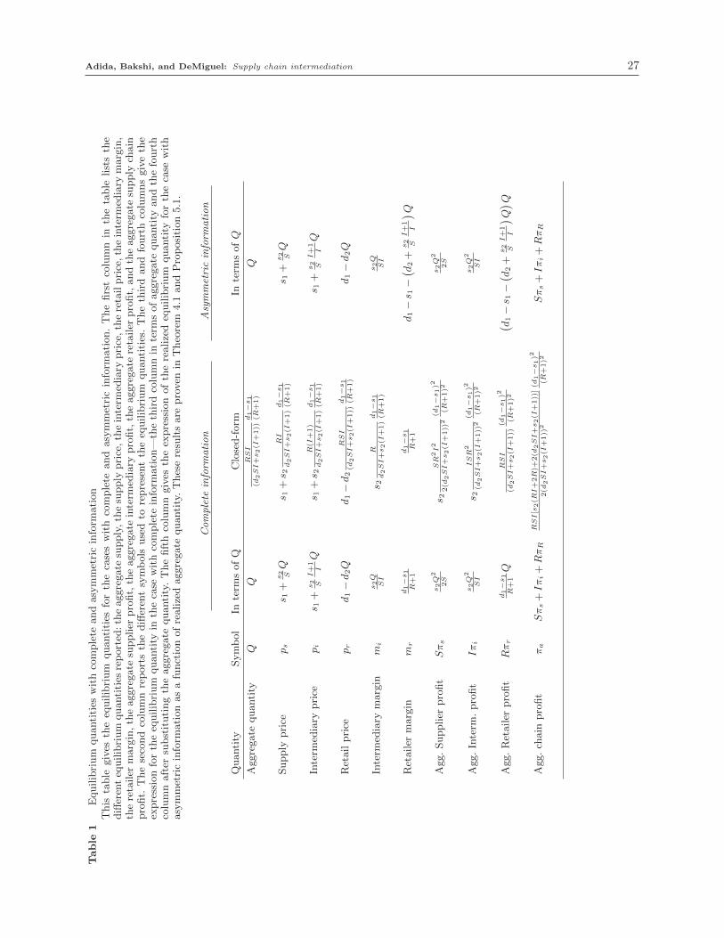
Adida, Bakshi, and DeMiguel: Supply chain intermediation 27
Table
1Equilibrium
quantities
withcomplete
andasymmetricinform
ation
This
table
gives
theequilibrium
quantities
forthecaseswith
complete
and
asymmetricinform
ation.Thefirstcolumn
inthetable
liststhe
differen
tequilibrium
quantities
reported
:theaggregate
supply,thesupply
price,theinterm
ediary
price,theretailprice,theinterm
ediary
margin,
theretailer
margin,theaggregate
supplier
profit,theaggregate
interm
ediary
profit,theaggregate
retailer
profit,andtheaggregate
supply
chain
profit.
Thesecondcolumnreportsthedifferen
tsymbols
usedto
representtheequilibrium
quantities.Thethirdandfourthcolumnsgivethe
expressionfortheequilibrium
quantity
inthecase
withcomplete
inform
ation—
thethirdcolumnin
term
sofaggregate
quantity
andthefourth
columnafter
substitutingtheaggregate
quantity.Thefifthcolumngives
theexpressionoftherealizedequilibrium
quantity
forthecase
with
asymmetricinform
ationasafunctionofrealizedaggregate
quantity.Theseresultsare
proven
inTheorem
4.1
andProposition5.1.
Complete
inform
ation
Asymmetricinform
ation
Quantity
Symbol
Interm
sofQ
Closed-form
Interm
sofQ
Aggregate
quantity
RSI
(d2SI+s2(I
+1))
d1−s1
(R+1)
Q
Supply
price
ps
s 1+
s2 SQ
s 1+s 2
RI
d2SI+s2(I
+1)d1−s1
(R+1)
s 1+
s2 SQ
Interm
ediary
price
pi
s 1+
s2 S
I+1
IQ
s 1+s 2
R(I
+1)
d2SI+s2(I
+1)d1−s1
(R+1)
s 1+
s2 S
I+1
IQ
Retailprice
pr
d1−d2Q
d1−d2
RSI
(d2SI+s2(I
+1))
d1−s1
(R+1)
d1−d2Q
Interm
ediary
margin
mi
s2Q
SI
s 2R
d2SI+s2(I
+1)d1−s1
(R+1)
s2Q
SI
Retailer
margin
mr
d1−s1
R+1
d1−s1
R+1
d1−s 1
−( d
2+
s2 S
I+1
I
) Q
Agg.Supplier
profit
Sπs
s2Q
2
2S
s 2SR
2I2
2(d
2SI+s2(I
+1))
2(d
1−s1)2
(R+1)2
s2Q
2
2S
Agg.Interm
.profit
Iπi
s2Q
2
SI
s 2ISR
2
(d2SI+s2(I
+1))
2(d
1−s1)2
(R+1)2
s2Q
2
SI
Agg.Retailer
profit
Rπr
d1−s1
R+1Q
RSI
(d2SI+s2(I
+1))
(d1−s1)2
(R+1)2
( d1−s 1
−( d
2+
s2 S
I+1
I
) Q) Q
Agg.ch
ain
profit
πa
Sπs+Iπi+RπR
RSI[s
2(R
I+2R)+
2(d
2SI+s2(I
+1))]
2(d
2SI+s2(I
+1))
2(d
1−s1)2
(R+1)2
Sπs+Iπi+RπR
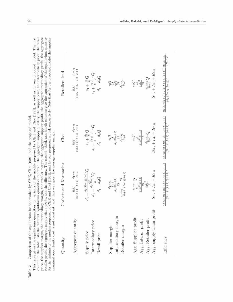
28 Adida, Bakshi, and DeMiguel: Supply chain intermediation
Table
2Comparisonoftheequilibrium
forthemodelsbyC&K,Choi[1991],andtheproposedmodel.
This
table
gives
theequilibrium
quantities
forvariants
ofthemodelsproposedbyC&K
andChoi[1991],aswellasforourproposedmodel.Thefirst
columnin
thetable
liststhedifferen
tequilibrium
quantities
reported
:theaggregate
supply
quantity,thesupply
price,theinterm
ediary
price,theretail
price,thesupplier
margin,theinterm
ediary
margin,theretailer
margin,theaggregate
supplier
profit,
theaggregate
interm
ediary
profit,
theaggregate
retailer
profit,theaggregate
supply
chain
profit,andtheeffi
cien
cy.Thesecond,third,andfourthcolumnsgivetheexpressionoftheequilibrium
quantity
fortheva
riants
ofthemodelsproposedbyC&K
andChoi[1991],andforourproposedmodel,resp
ectively.
Note
thatforourproposedmodel
thesupplier
marginalopportunitycost
isnotconstant,
andthuswereport
theav
eragesupplier
margin.
Quantity
Corbettan
dKarmarkar
Choi
Retailers
lead
Agg
regatequan
tity
RSI
d2(S
+1)(I+1)d1−s1
R+1
RSI
d2(S
+1)(I+1)d1−s1
R+1
RSI
(d2SI+s2(I
+1))
d1−s1
R+1
Supply
price
d1−
d2(R
+1)(I+1)
RI
Qs 1
+d2 SQ
s 1+
s2 SQ
Interm
ediary
price
d1−
d2(R
+1)
RQ
s 1+
d2 SS+I+1
IQ
s 1+
s2 SI+1
IQ
Retailprice
d1−d2Q
d1−d2Q
d1−d2Q
Supplier
margin
d1−s1
S+1
d2Q
Ss2Q
2S
Interm
ediary
margin
d2Q(R
+1)
RI
d2Q(S
+1)
SI
s2Q
SI
Retailermargin
d1−s1
R+1
IS
(I+1)(S+1)
d1−s1
R+1
d1−s1
R+1
Agg
.Supplier
profit
d1−s1
S+1Q
d2Q
2
Ss2Q
2
2S
Agg
.Interm
.profit
d2Q
2(R
+1)
RI
d2Q
2(S
+1)
SI
s2Q
2
SI
Agg
.Retailerprofit
d2Q
2
Rd1−s1
R+1Q
d1−s1
R+1Q
Agg
.supply
chainprofit
Sπs+Iπi+RπR
Sπs+Iπi+RπR
Sπs+Iπi+RπR
Efficien
cy4SIR(R
I+RS+SI+R+S+I+1)
(S+1)2
(I+1)2
(R+1)2
4SIR(R
I+RS+SI+R+S+I+1)
(S+1)2
(I+1)2
(R+1)2
RI[s
2R(I
+2)+
2(d
2SI+s2(I
+1))]
(d2SI+s2(I
+1))
22d2S+s2
(R+1)2

Adida, Bakshi, and DeMiguel: Supply chain intermediation 29
Table 3 Monotonicity properties
This table gives the monotonicity properties of the equilibrium quantities. The first column in the table lists thedifferent equilibrium quantities for which we report the monotonicity properties: the aggregate supply, the supplyprice, the intermediary price, the retail price, the intermediary margin, the retailer margin, the supplier profit, theintermediary profit, and the retailer profit. The second column reports the different symbols used to represent theequilibrium quantities. The next five columns give the monotonicity relation of each equilibrium quantity to thenumber of suppliers (S), the number of intermediaries (I), the number of retailers (R), the supply sensitivity (s2),and the demand sensitivity (d2), respectively, where the symbol “+” (“−”) indicates that the equilibrium quantityincreases (decreases) with respect to the parameter, and “∩” indicates that the equilibrium quantity is unimodal withrespect to the parameter. The results in this table are proven in Theorem 4.2.
Quantity Symbol S I R s2 d2
Aggregate quantity Q + + + − −Supply price ps − + + + −Intermediary price pi − − + + −Retail price pr − − − + −Intermediary margin mi − − + + −Retailer margin mr 0 0 − 0 0
Supplier profit πs − + + ∩ −Intermediary profit πi ∩ − + ∩ −Retailer profit πr + + − − −
Table 4 Effect of asymmetric information on equilibrium quantities
This table shows the effect of asymmetric information about supply sensitivity on the equilibrium quantities. The firstcolumn lists the different equilibrium quantities for which we report the relation: the aggregate supply, the supplyprice, the intermediary price, the retail price, the intermediary margin, the retailer margin, the supplier profit, theintermediary profit, and the retailer profit. The second column reports the different symbols used to represent theequilibrium quantities. The third column shows the effect for the case where the realized sensitivity is low (s2 = sL2 ).The fourth column for the case where the realized sensitivity is high and the prior probability of low sensitivity is low(s2 = sH2 and ν < ν0). The fifth column for the case where the realized sensitivity is high and the prior probability oflow sensitivity is high (s2 = sH2 and ν > ν0). The symbol “+” (“−”) indicates that the equilibrium quantity is larger(smaller) in the supply chain with asymmetric information. The results in this table are proven in Proposition 5.2.
Quantity Symbol Low sensitivity High sensitivity High sensitivity
ν < ν0 ν > ν0
Aggregate quantity Q + − −Supply price ps + − −Intermediary price pi + − −Retail price pr − + +
Intermediary margin mi + − −Retailer margin mr − + +
Supplier profit πs + − −Intermediary profit πi + − −Retailer profit πr − + −
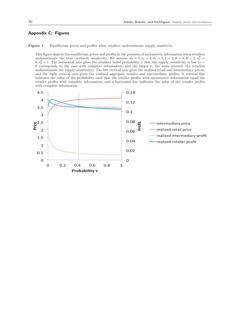
30 Adida, Bakshi, and DeMiguel: Supply chain intermediation
Appendix C: Figures
Figure 1 Equilibrium prices and profits when retailers underestimate supply sensitivity
This figure depicts the equilibrium prices and profits in the presence of asymmetric information when retailersunderestimate the true (realized) sensitivity. We assume d2 = 1, s1 = 3, d1 = 5, I = 2, S = 3,R = 2, sH2 =6, sL2 = 1. The horizontal axis gives the retailers belief probability ν that the supply sensitivity is low (ν =0 corresponds to the case with complete information, and the larger ν, the more severely the retailersunderestimate the supply sensitivity). The left vertical axis gives the realized retail and intermediary prices,and the right vertical axis gives the realized aggregate retailer and intermediary profits. A vertical lineindicates the value of the probability such that the retailer profits with asymmetric information equal theretailer profits with complete information, and a horizontal line indicates the value of the retailer profitswith complete information.
!"
!#!$"
!#!%"
!#!&"
!#!'"
!#("
!#($"
!#(%"
!"
!#)"
("
(#)"
$"
$#)"
*"
*#)"
%"
%#)"
!" !#$" !#%" !#&" !#'" ("
!"#$
%&
!"'()&
!"#*+*','%-&.&
+,-./0.1+2/3"4/+5."
/.26+7.1"/.-2+6"4/+5."
/.26+7.1"+,-./0.1+2/3"4/89-"
/.26+7.1"/.-2+6./"4/89-"

Adida, Bakshi, and DeMiguel: Supply chain intermediation 31
ReferencesAdida, E., V. DeMiguel. 2011. Supply chain competition with multiple manufacturers and retailers. Opera-
tions Research 59(1) 156–172.
Alberts, H.R. 2010. Billionaire brothers tie up with Walmart. Forbes.
Anand, K.S., H. Mendelson. 1997. Information and organization for horizontal multimarket coordination.Management Science 43(12) 1609–1627.
Belavina, E., K. Girotra. 2011. Global sourcing through intermediaries. Forthcoming in Management Science.
Bernstein, F., A. Federgruen. 2005. Decentralized supply chains with competing retailers under demanduncertainty. Management Science 51(1) 18–29.
Biglaiser, G. 1993. Middlemen as experts. The RAND Journal of Economics 24(2) 212–223.
Cachon, G.P., M.A. Lariviere. 2005. Supply chain coordination with revenue-sharing contracts: strengthsand limitations. Management Science 51(1) 30–44.
Carr, S.M., U.S. Karmarkar. 2005. Competition in multi-echelon assembly supply chains. ManagementScience 51(1) 45–59.
Cheng, W.-G. 2010. Li & Fung signs Walmart deal that may generate $2 billion sales. Business Week.
Cho, S.H. 2011. Horizontal mergers in multi-tier decentralized supply chains. Tepper School of Businessworking paper.
Choi, S.C. 1991. Price competition in a channel structure with a common retailer. Marketing Science 10(4)271–296.
Corbett, C.J., U.S. Karmarkar. 2001. Competition and structure in serial supply chains with deterministicdemand. Management Science 47(7) 966–978.
Correa, J.R., N. Figueroa, N.E. Stier-Moses. 2011. Pricing with markups in industries with increasingmarginal costs. Columbia GSB working paper.
Cottle, R.W, J.-S. Pang, R.E. Stone. 2009. The Linear Complementarity Problem. Society for Industrialand Applied Mathematics, Philadelphia.
Einhorn, B. 2010. Li & Fung: a factory sourcer shines. Business Week.
Farahat, A., G. Perakis. 2009. Profit loss in differentiated oligopolies. Operations Research Letters 37(1)43–46.
Farahat, A., G. Perakis. 2011. Technical note—A comparison of Bertrand and Cournot profits in oligopolieswith differentiated products. Operations Research 59(2) 507–513.
Fung, V.K., W.K. Fung, Y. Wind. 2008. Competing in a Flat World: Building Enterprises for a BorderlessWorld . Wharton School Publishing, Philadelphia.
Fung Group. 2012. Since 1995: A multinational group emerges. http://www.funggroup.com/eng/about/
heritage_1995.php.
Goyal, M., S. Netessine. 2007. Strategic technology choice and capacity investment under demand uncer-tainty. Management Science 53(2) 192–207.
Griffin, J.M. 1972. The process analysis alternative to statistical cost functions: An application to petroleumrefining. The American Economic Review 62(1/2) 46–56.
Ha, A., S. Tong, H. Zhang. 2011. Sharing demand information in competing supply chains with productiondiseconomies. Management Science 57(3) 566–581.
Hackner, J. 2003. A note on price and quantity competition in differentiated oligopolies. Journal of EconomicTheory 93(2) 223–239.
Kalai, E., M.I. Kamien, M. Rubinovitch. 1992. Optimal service speeds in a competitive environment. Man-agement Science 38(8) 1154–1163.
Knowledge@Wharton. 2007. Li and Fung’s Bruce Rockowitz: Managing supply chains in a ‘flat’ world. http://www.knowledgeatwharton.com.cn/index.cfm?fa=viewfeature&articleid=1656&languageid=1.
Lafontaine, F., M. Slade. 2012. Inter-firm contracts. R. Gibbons, J. Roberts, eds., The Handbook of Orga-nizational Economics. Princeton University Press, 958–1013.
32 Adida, Bakshi, and DeMiguel: Supply chain intermediation
Lariviere, M., E. Porteus. 2001. Selling to the newsvendor: An analysis of price-only contracts. Manufacturing& Service Operations Management 3(4) 293–305.
Majumder, P., A. Srinivasan. 2008. Leadership and competition in network supply chains. ManagementScience 54(6) 1189–1204.
McFarlan, F.W., W. Kirby, T. Manty. 2007. Li & Fung 2006. Harvard Business School Teaching Case.
Mollick, A.V. 2004. Production smoothing in the Japanese vehicle industry. International Journal of Pro-duction Economics 91(1) 63–74.
Netessine, S., F. Zhang. 2005. Positive vs. negative externalities in inventory management: Implications forsupply chain design. Manufacturing & Service Operations Management 7(1) 58–73.
Perakis, G., G. Roels. 2007. The price of anarchy in supply chains: Quantifying the efficiency of price-onlycontracts. Management Science 53(8) 1249–1268.
Porteus, E.L. 2002. Foundations of stochastic inventory theory . Stanford University Press, Stanford, CA.
Reuters. 2012. Li and Fung in talks to buy NY-based sourcing company. http://www.reuters.com/
article/2012/10/04/us-liandfung-synergies-idUSBRE8931BM20121004.
Rubinstein, A., A. Wolinsky. 1987. Middlemen. The Quarterly Journal of Economics 102(3) 581.
Singh, N., X. Vives. 1984. Price and quantity competition in a differentiated duopoly. The RAND Journalof Economics 15(4) 546–554.
Spengler, J. 1950. Vertical integration and antitrust policy. Journal of Political Economy 58 347–352.
The Telegraph. 2012. Li & Fung—the Made in China giant you have never heard of. The Telegraph.
Varian, H.R. 1992. Microeconomic analysis. Norton, New York. Third edition.
Vives, X. 1999. Oligopoly Pricing. Old Ideas and New Tools. MIT Press, Cambridge.
Wu, S.D. 2004. Supply chain intermediation: a bargaining theoretic framework. D. Simchi-Levi, S.D. Wu,Z.M. Shen, eds., Handbook of Quantitative Supply Chain Analysis: Modelling in the E-Business Era.Kluwer Academic Publishers, Amsterdam, 67–115.
Adida, Bakshi, and DeMiguel: Supply chain intermediation 33
Supplemental file

34 Adida, Bakshi, and DeMiguel: Supply chain intermediation
Appendix D: The case with convex increasing marginal opportunity cost
We now show that πi is unimodal in S even for the following more general marginal opportunity
cost function:
ps(q) = s1 + s2qθ; for θ≥ 1.
Note that this is a convex increasing monomial function.
The supplier’s profit is:
πs,j = ps(qs,j)qs,j −∫ qs,j
0
(s1 + s2qθ)dq=
s2θqθ+1s,j
θ+1.
The intermediary’s decision is:
maxqi,l
[pi −
[s1 + s2
(qi,l +Qi,−l
S
)θ]]
qi,l.
The first-order conditions imply:
pi −[s1 + s2
(qi,l +Qi,−l
S
)θ]− s2θ
S
(qi,l +Qi,−l
S
)θ−1
qi,l = 0;
which implies:
pi = s1 + s2
(Q
S
)θ
+s2θ
I
(Q
S
)θ
;
and the margin, mi of the intermediary is:
mi = pi − ps =s2θ
I
(Q
S
)θ
;
and the profit, πi, of each intermediary is:
πi =mi
Q
I=
s2θS
I2
(Q
S
)θ+1
.
The retailer’s decision problem can be stated as:
maxqr,k
(pr − pi)qr,k =
[d1 − d2(qr,k +Qr,−k)−
[s1 + s2
(Q
S
)θ
+s2θ
I
(Q
S
)θ]]
qr,k.
The first order conditions then imply:
Φ(Q,S) = d2
(1+
1
R
)Q+ s2
(1+
θ
I
)(1+
θ
R
)(Q
S
)θ
− (d1 − s1) = 0.
Now we are ready to determine whether πi is unimodal in S. We first calculate dπi/dS:
dπi
dS=
(∂πi
∂Q
)dQ
dS+
∂πi
∂S=
(Q
S
)θs2θ
I2
[(θ+1)
dQ
dS− θ
Q
S
];
Adida, Bakshi, and DeMiguel: Supply chain intermediation 35
where dQ/dS can be determined using the following relationship:
dΦ
dS=
∂Φ
∂Q
dQ
dS+
∂Φ
∂S= 0;
which implies:
dQ
dS=
s2θ(1+ θ
I
) (1+ θ
R
)(Qθ
Sθ+1
)
d2(1+ 1
R
)+ s2θ
(1+ θ
I
) (1+ θ
R
)(Qθ−1
Sθ
) =QS
1+
(d2(R+1)
s2θR(1+ θI )(1+
θR)
)(Sθ
Qθ−1
) <Q
S. (14)
Substituting the above relationship in the expression for dπi/dS and evaluating the terms we
conclude that dπi/dS < 0 if and only if dQ/dS < θQ/((θ+1)S) or equivalently, if and only if:
1
1+
(d2(R+1)
s2θR(1+ θI )(1+
θR)
)(SQ
)θ−1
S
<θ
θ+1.
Also note that:
d(QS
)
dS=
1
S
(dQ
dS− Q
S
)< 0 =⇒
d(
SQ
)
dS> 0.
Hence, it is easy to verify that:
d
dS
1
1+
(d2(R+1)
s2θR(1+ θI )(1+
θR)
)(SQ
)θ−1
S
< 0.
This implies that, as S is increased, then dπi/dS can change sign from positive to negative at most
once. In other words πi is unimodal in S.
We also show that for this marginal opportunity cost function the retailer margin does depend on
the number of suppliers and of intermediaries, as opposed to the case of a linear function. Indeed,
mr = d1 − d2Q− s1 − s2
(1+
θ
I
)(Q
S
)θ
anddmr
dS=
∂mr
∂Q
dQ
dS+
∂mr
∂S,
where∂mr
∂S=
s2S
(1+
θ
I
)(Q
S
)θ
,
and∂mr
∂Q=−d2 − s2
S
(1+
θ
I
)(Q
S
)θ−1
.
Since both of the two expressions above are independent of R but dQ/dS does depend on R when
θ > 1, as is apparent from (14), it is clear that dmr/dS 6= 0 in general.
Similarly,dmr
dI=
∂mr
∂Q
dQ
dI+
∂mr
∂I,
36 Adida, Bakshi, and DeMiguel: Supply chain intermediation
where∂mr
∂I=
s2θ
I2
(Q
S
)θ
.
dQ/dI can be deduced from the first order conditions
Ψ(Q,I) = d2
(1+
1
R
)Q+ s2
(1+
θ
I
)(1+
θ
R
)(Q
S
)θ
− (d1 − s1) = 0
and the relationship:dΨ
dI=
∂Ψ
∂Q
dQ
dI+
∂Φ
∂I= 0;
which implies:
dQ
dI=
s2θI2
(1+ θ
R
) (QS
)θ
d2(1+ 1
R
)+ s2θ
(1+ θ
I
) (1+ θ
R
)(Qθ−1
Sθ
) =QI2
1+ θI+(
d2(R+1)
s2θ(R+θ)
)(Sθ
Qθ−1
) . (15)
Since both ∂mr/∂I and ∂mr/∂Q are independent of R but dQ/dI does depend on R when θ > 1,
as is apparent from (15), it is clear that dmr/dI 6= 0 in general.