SUPPLY CHAIN MANAGEMENT: A SYSTEM DYNAMICS APPROACH …

117

Journal of ICT, 10, pp: 117–135

SUPPLY CHAIN MANAGEMENT: A SYSTEM DYNAMICS APPROACH TO IMPROVE VISIBILITY AND PERFORMANCE

Chan Kah Wai1

Ang Chooi-Leng

Department of Applied SciencesCollege of Arts and SciencesUniversiti Utara Malaysia

[email protected]

ABSTRACT

Competitiveness is one of the factors successful organizations excel in, and they will do anything necessary to gain an edge over their competitors. The system dynamics approach to simulation modelling is being considered as one of the methods to increase competitiveness. System dynamics is essentially a methodology suited to studying and managing complex feedback systems and provides a means for understanding the causes of industry behaviour. This research builds a complete system dynamics model for internal supply chain events (from order to ship-out) from the perspectives of a semiconductor company. System dynamics models are simulation-based models that allow the investigation and identification of discrepancies between the business policy and the actual practice of key events as well as provide a better visibility of the company’s system. With the understanding of the internal workings of the supply chain system, experiments with the simulation model could provide alternative configurations to achieve better performance. This research utilizes system dynamics to better understand the supply chain system and with it, to find better solutions through experimentations with a few key variables in the supply chain system. The result of this research reveals that the company could achieve 25% reduction in inventory cost should the recommendations be followed.

Keyword: Supply chain, System dynamics, Simulation, Supply chain optimization, Supply chain visibility, Semiconductor, Manufacturing, Warehouse, Model experiment, Bullwhip effect.


118

INTRODUCTION

The competition between organizations is well known in the semiconductor industry. This research focuses on a semiconductor company that is well known for its microprocessor chips for personal computers. This research is conducted at one of its plants located in Penang, Malaysia. Most organization nowadays are confronted with a saturated, maturing market (Inagaki & Kuroda, 2007) as well as competitors outsourcing to lower-cost countries (Levans, 2002). Companies and factories have to look for ways to improve their business in order to increase their competitiveness.

The focus of improvement has gradually shifted away from looking at competitors, but instead to suppliers and distributors, or more precisely, the supply chain. Business executives and managers recognize that the ultimate success of any enterprise is no longer built around a firm’s capability and capacity, but on a supply chain’s capability and capacity (Chow, Madu, Kuei, Lu, Lin & Tseng, 2006). The supply chain is a linked set of resources and processes that begin with the sourcing of raw materials and extend through to the delivery of end items to the final customer (Trkman, Stemberger, Jachlic & Groznik, 2007; Stevens, 1989). The supply chain is being looked at with renewed interest as the drive for efficiency affects the semiconductor industry.

There are various researches into the field of supply chain management such as supply chain flexibility by Fantasy and Kumar, (2006) and reverse (also called close loop) supply chain by Kumar and Yamaoka (2007). Most supply chain problems can be related to communication and information issues, inventory issues and business process issues. Most of these issues require understanding of the supply chain beyond the viewpoint of the supply chain manager. The complexity of a supply chain can best be understood from a systemic point of view, such as system dynamics modelling. This research aims improve and help decision-making in the managerial aspects of the supply chain system by modelling the internal events of the supply chain system of a semiconductor company.

THE SEMICONDUCTOR COMPANY’S SUPPLY CHAIN ISSUES

The company has been practising a lot of management principles especially postponement strategies and supply chain management (SCM). It is concerned about the overall performance of the supply chain system and wishes for a thorough study on it. It is also concerned about the effective implementation of some of the company’s policies. The company supplies components

119


to customers of various sorts all over the world. Some have factories and plants in different parts of the world. Thus, its supply chain system, a system of information and material flow, is very important. The supply chain is an important part of the management, which is made up of material suppliers, production facilities, distribution services, and customers (Stevens, 1989). In order to manage the supply chain effectively, it should be properly modelled and its processes integrated and coordinated into the model (Vernadat, 1996).

A supply chain is a linked set of resources and processes that begins with the sourcing of raw materials and extends through to the delivery of the end items to the final customer (Trkman et al., 2007). A supply chain model of a semiconductor company with its entire components is very complex. Parts of the system, such as capacity planning, require the manager to make decisions based on the company policy and the information on demands. Thus, a decision factor decides the responses and condition of the supply chain. Overreactions, unnecessary interventions, second guessing, mistrust, and distorted information throughout a supply chain increase the chaos in the company (Christopher & Lee, 2001). Ge, Yang Proundlove and Spring, (2004) implies that this uncertainty affects the management and particularly the production floor managers in a way that influences them to inflate the safety stocks and the inventory across various assembly test and warehouses. Optimization and the efficient use of the supply chain are reduced as a result. A short product lifespan coupled with high customer expectation that the product will run flawlessly require elaborate planning and an effective and efficient production structure.

A SUPPLY CHAIN SYSTEM SIMULATION MODEL

A simulation model allows a supply chain system to be viewed in a holistic manner. Irani, Hlupic, Buldmin and Love, (2000) argued that in order to get a better understanding and have a holistic approach to business, model simulation is the way. Take a system that may be hard to understand or dangerous to manipulate, and simulation can render it in a form that is easier to understand and safer to play with (Taylor, 2004). A simulation model can represent a supply chain system in a computer system with all its components as well. Taylor (2004) points out that a simulation model uses software objects to represent components of a business and the result of their interaction is tested by running the model. Once the final model has been finalized, it can be used to analyse various production alternatives as in the case of Irani et al. (2000) and Greasly and Barlow (1998).


120

The specific objectives are:

• build a system dynamics model for internal supply chain events (from order to ship-out); and

• investigate and identify discrepancy between the business policy and the actual practice of key events in order to achieve the supply chain optimization.

APPROACH TO MODELLING AND SIMULATION

The research methodology is based on model experimentation. It adjusts and stimulates settings to achieve supply chain optimization. Taylor (2004) defines simulation as a tool that could render a system that may be hard to understand or dangerous to manipulate, into a form that is easier to understand and safer to play with. When it comes to the characteristics of a system, we have to determine if the system is purely a quantitative model, qualitative model or a combination of both. Discrete event simulation (DES) is inclined towards quantitative aspects (Eldabi, Iran, Paula And Love, 2002). System Dynamics (SD) are comfortable with qualitative aspects arising from the complexity of the system (Sweetser, 1999). A choice of which approach to simulation modelling has to be made based on the strengths and weaknesses of each approach.

The unique properties of a SD system as described by Sweetser (1999) are listed below:

• well suited to modelling continuous processes;• can model system where behaviour changes in a non-linear fashion;• are able to cope with extensive feedbacks occurring within the system;• is often used in strategic policy analysis;• incorporates “fuzzy” qualitative aspects of behaviour that, while difficult

to quantify, might significantly affect the performance of a system; and• is better at modelling non-linear relationships, feedback loops, and

continuous systems.

The company in this study is trying to look at the supply chain at a strategic level. To do this, it is looking at a product throughout its life cycle, which is about one and a half years. The production process is also governed by a production policy that is based on a feedback system. Each part of the supply chain has an influence on each other and their relationship is complex. The supply chain system behaviour is identified as non-linear and influenced by

121


feedback loops which are continuous in nature. Based on this analysis of the supply chain, a System Dynamics approach is the more appropriate approach as it can incorporate each aspect of the supply chain system.

Data Source and Collection

As the methodology of this research is based on a simulation model, detailed knowledge of how the supply chain works and what factors contribute to the characteristics of the system have to be known. There is a need for data on the production floor as well as the inventory warehouse. The focus of this research is on a product codenamed C2D. This product is the current best-selling product and it is almost at the end of its life cycle. The main bulk of the data came from secondary sources within the company’s database. Most of these data were collected on a weekly basis and time-sensitive data have a cut-off point at every Saturday 6.00pm GMT +8. The only data set collected monthly was the demand forecast. The data were collected within a time frame of January 2007 till June 2008. This time frame was chosen, because based on the experience with previous similar product lines, the product life cycle was expected to be one and a half years. These data sets combined with a time frame of one and a half years reflect on the characteristics and the properties of C2D. In total, ten sets of data were collected. Besides secondary data, interviews and meetings were set up to obtain professional views on the supply chain system and feedbacks on the reliability of the model to reflect the real system. The statements were not recorded officially but were used to shape our perceptions and understanding of the supply chain system.

Planning Department

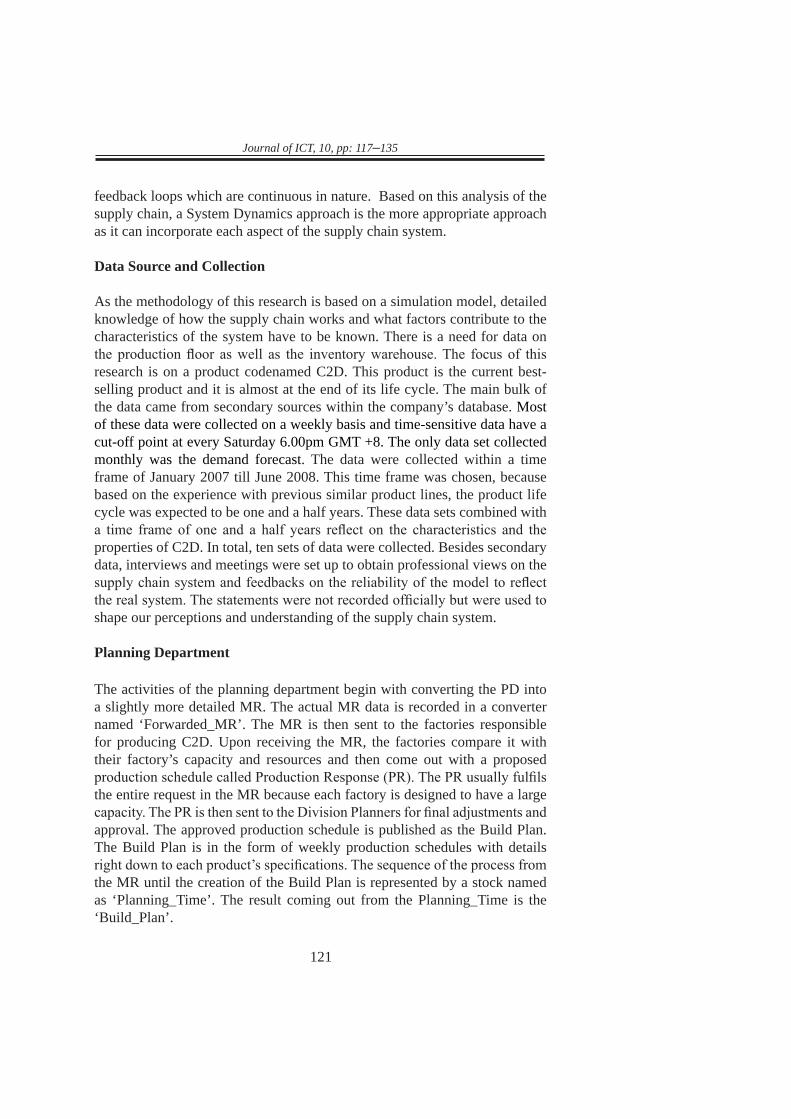
The activities of the planning department begin with converting the PD into a slightly more detailed MR. The actual MR data is recorded in a converter named ‘Forwarded_MR’. The MR is then sent to the factories responsible for producing C2D. Upon receiving the MR, the factories compare it with their factory’s capacity and resources and then come out with a proposed production schedule called Production Response (PR). The PR usually fulfils the entire request in the MR because each factory is designed to have a large capacity. The PR is then sent to the Division Planners for final adjustments and approval. The approved production schedule is published as the Build Plan. The Build Plan is in the form of weekly production schedules with details right down to each product’s specifications. The sequence of the process from the MR until the creation of the Build Plan is represented by a stock named as ‘Planning_Time’. The result coming out from the Planning_Time is the ‘Build_Plan’.


122

The iThink System Dynamics Simulation Model

Figure 1. Simulation Model using iThink.Figure 1. Simulation Model using iThink.

123


Production Centre

After the A&T process, the products will either be kept in a semi-finished goods inventory (SFGI) or go straight to the packaging process. The quantities flowing out of A&T are captured with a converter named ‘Batch_Total’. The ‘SFGI_Flow’ is governed by a converter named ‘SFGI_Stockage’. The SFGI_Stockage is a set of data taken directly from the SFGI data. The amount of products going straight to the packaging process depends on how much of the products from A&T flow to SFGI. The amount is the net of A&T transit (captured using Batch_Total) minus SFGI_Stockage. The SFGI starts operation only in the thirty-seventh week of production. The packaging process is represented by a stock named ‘Packaging’. Packaging receives products from two flows, named ‘SFGI_Shipout’ and A&T Direct. A&T Direct represents the flow of the remaining products from A&T that are not sent to the SFGI. Packaging has a process time of one day. After the packaging process, the finished goods are sent to the main inventory (CW) through a flow named Final_Product.

CW and Hubs Inventory

The movement of the products from CW to the customers is represented by a flow named ‘CW_to_Customers’. The movement of the products from CW to Hubs is represented by a flow named ‘Shipout_to_Hubs’. The flow of the products from CW to customers is governed by a converter named ‘CW_Customer_Fulfilment’. In the absence of a concrete order fulfilment structure, the ship-out data from CW to customers is used as the CW customer fulfilment. CW to Customers data set is recorded into CW_Customer_Fulfilment.

‘Shipout_to_Hubs’ is governed by a converter named ‘CW_to_Hubs#’. CW_to_Hubs# uses real data from CW to Hubs. A stock named ‘Hubs’ stores all the products flowing into Hubs. Just like the CW customer fulfilment, Hubs use real data of Hubs customer fulfilment, recorded in a converter named ‘Hubs_Customers_Fulfilment’. The flow of products out of Hubs to Customers is represented by a flow named ‘Hubs_to_Customers’. The flow of Hubs to Customers is governed by Hubs_Customers_Fulfilment. As Hubs starts operation on the twenty second week, the data set in the Hubs_Customers_Fulfilment from the first week to the twenty-first week is set to zero. This stops the function of Hubs for that period.

Production Think Tank

The production think tank is the most sophisticated part of the supply chain model. It makes decisions on what, when and how much to produce. It makes these decisions based on a variety of factors such as the PD and the


124

target inventory level. The main decision of the production think tank is the production policy. It is represented by a converter named ‘Production_Policy’. In Production_Policy, the decision formula is represented by:

IF(shortage<0) THEN(Projected_Demand*1) ELSE(Projected_Demand*1.2)

This formula checks on the condition of shortage; whether there is a shortage of inventory based on the definition of WOI. If there is no shortage, (indicated by a number smaller than 0), then Projected_Demand is used for MR. If there is a shortage, (indicated by the number 0 or larger), then MR will be made using the formula Projected_Demand*1.2. Shortage is defined as the target inventory minus the CW level. It is represented by a converter named ‘Shortage’. If the inventory level in CW is larger than the target inventory, then Shortage will be less than zero. If the inventory level in CW is smaller than the target inventory, then Shortage will have a positive integer number. The target inventory is represented by a converter named ‘Target_Inventory’. It receives three different types of information to create the target inventory. The formula in Target_Inventory is:

IF(TIME<5) THEN (HISTORY(Judged_Demand, TIME=1) *WOI_modifier) ELSE(Moving_Average*WOI_modifier)

Moving_Average takes the historical data of the past four weeks from PD and averages the numbers. This figure is then used as the base for calculating the target inventory. The formula for Moving average is:

MEAN(time_n’1,time_n’2,time_n’3,time_n’4)

The production policy, after taking into account all these factors, creates MR. MR is sent to the Planning Department for further action. The cycle continues again from this point onwards.

Customers

The Customers receive products from both the CW and the Hubs. Customers are represented by a stock named ‘Customers’. The products movement from the CW is represented by a flow named CW_to_Customers and this is governed by the ‘converter’ CW_Customer_fulfilment. As for the movement of the products from the Hubs to the Customers, it is represented by a flow

125


named Hubs_to_Customers. Hub_to_Customers is governed by a converter named Hubs_Customers_Fulfilment. The Customers represent the computer assemblers and the retailers in the supply chain system.

Model Validation and Adjustments

The first validation test is performed with the model variables and the characteristics set using the actual supply chain system data. Using the CW inventory level as the measurement of conformity, a paired sample t-test yields a p-value of 0.94. Using a 0.01 level of significance (α-value = 0.01), it implies that there is no significant difference between the simulated CW Inventory level and the actual CW Inventory level. Furthermore, the large p-value, close to 1, implies that these two sets of data have a high level of similarity. This shows that the simulation model is successful in capturing the behaviour and the characteristics of the actual supply chain system.

The second validation test runs the full model with the production think tank as the main processing centre that allows the model to regulate itself. The result shows the simulation run is significantly different from the actual supply chain, but the overall pattern is maintained. Readjustments are made to the time frame of the simulation run, reducing it from 18 months to 12 months. This adjustment takes out the ramp- up period of the product, making the production process smoother.

The new simulation model time frame starts from June 2007 to June 2008. The new model retains all the previous parameters while changing the time frame of the simulation run. A paired sample t-test gives a result with a p-value of 0.04. Using a 0.01 level of significance (α-value = 0.01), the result implies that there is no significant difference between the simulated CW Inventory level and the Actual CW inventory.

DISCREPANCY ANALYSIS

The simulation model that has been finalized in the validation process is taken as the base model for every experimentation and comparison hereafter. The main business policy that the semiconductor company tries to enforce is the policy regarding the WOI level. This policy states that the WOI level is to be maintained at 2.5 times the 4-point moving average of PD. This basically translates to maintaining a level of inventory which has a total of 2.5 times the forecasted sales. The base model was looked into to assess whether this policy


126

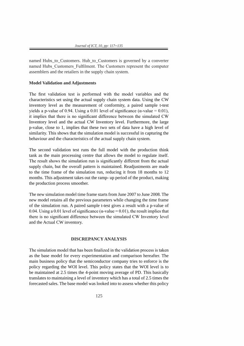
is adhered to or not. This test uses a comparison between the WOI policy and the simulated CW WOI. The CW WOI comparison chart and statistics are shown in Figure 2 and Table 1 respectively.

Figure 2. Simulated CW WOI level.

Table 1

Simulated CW WOI Statistics

Simulated CW WOI

Mean 3.8182692Standard Error 0.1745174Median 3.35Mode 3.14Standard Deviation 1.2584627Sample Variance 1.5837283Kurtosis 1.7892585Skewness 1.3524249Range 5.61Minimum 2.04Maximum 7.65Sum 198.55Count 52

A visual analysis of Figure 2 reveals that CW WOI level is above the stated WOI = 2.5 most of the time. The only time it went below the 2.5 level was from week14 to week18. The statistics of CW WOI (Table 1) reveal that the

Figure 2. Simulated CW WOI level.

0

5

10

1 3 5 7 9 11 13 15 17 19 21 23 25 27 29 31 33 35 37 39 41 43 45 47 49 51

WOI Policy Simulated CW WOI

127


mean of CW WOI is 3.82, which is well above the desired level of 2.5. It even has a maximum CW WOI level of 7.65. The observations of Figure 2 and the statistics revealed in Table 1 imply that the WOI policy of 2.5 was rarely adhered to and was exceeded for much of the model time frame. The semiconductor company has more inventory than it intends to keep for most of the time. There exists a discrepancy between the WOI policy and the actual practice.

MODEL EXPERIMENTATION

Experimentation with the Production Policy

The production policy for the base model is made of this formula:

IF(shortage<0) THEN(Projected_Demand*1) ELSE(Projected_Demand*1.2)

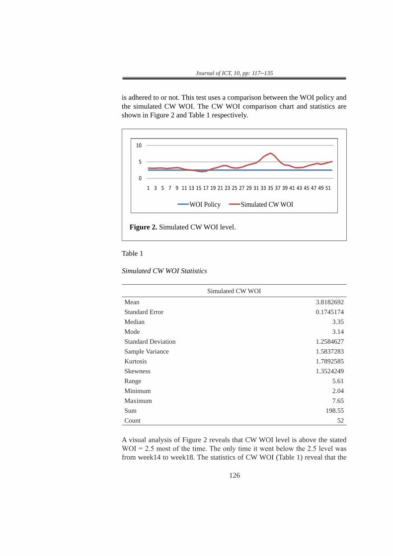
Two parameters are available for manipulation in this formula. These parameters have the values of ‘1’ and ‘1.2’ in this formula. ‘1’ signifies 100% and ‘1.2’ signifies 120%. The formula simply means that if there is no shortage, then it produces the projected demand, or else produces 120% of the projected demand. By changing the values, either one at a time or simultaneously, a set of scenarios are available for experimentation. These scenarios are a set of feasible variables for the simulation run. The results of these scenarios are summarized in Table 2. Throughout this entire experimentation, the WOI modifier was kept constant. Comparison among these scenarios shows that the best result is achieved by Scenario 3. It has an average WOI of 2.72 and Average Cycle Time of 2.66. Figure 3 shows the CW Inventory level of Scenario 3 along with the target inventory level and the total customer fulfilments.

Table 2

Production Policy Experimentation

Production Policy Average WOI Average Cycle Time

IF shortage then 1, Else 1.2 3.82 3.67

(Base model)

IF shortage then 0.9, Else 1.2 2.91 2.86 (Scenario 1)

(continued)


128

Production Policy Average WOI Average Cycle Time

IF shortage then 1, Else 1.1 3.47 3.35 (Scenario 2)

IF shortage then 0.9, Else 1.1 2.72 2.66 (Scenario 3)

Figure 3. Scenario 3 - If shortage, then 0.9, Else 1.1.

Experimentation with WOI Modifier

The WOI modifier is a parameter set at a constant value of 2.5 throughout the entire simulation model run for validation. It is considered a company’s policy set to maintain a healthy level of inventory to meet customers’ demand. In this part of the experimentation, we changed this value with a set of scenarios to try improving the performance of CW. Since increasing this value would only add more stocks in the inventory, a decreased value was chosen for the scenario. A set of feasible scenarios was created for the simulation run. The results of these scenarios run in the simulation model are shown in Table 3. Throughout this entire experimentation, the Production Policy parameters were kept constant as those of the base model.

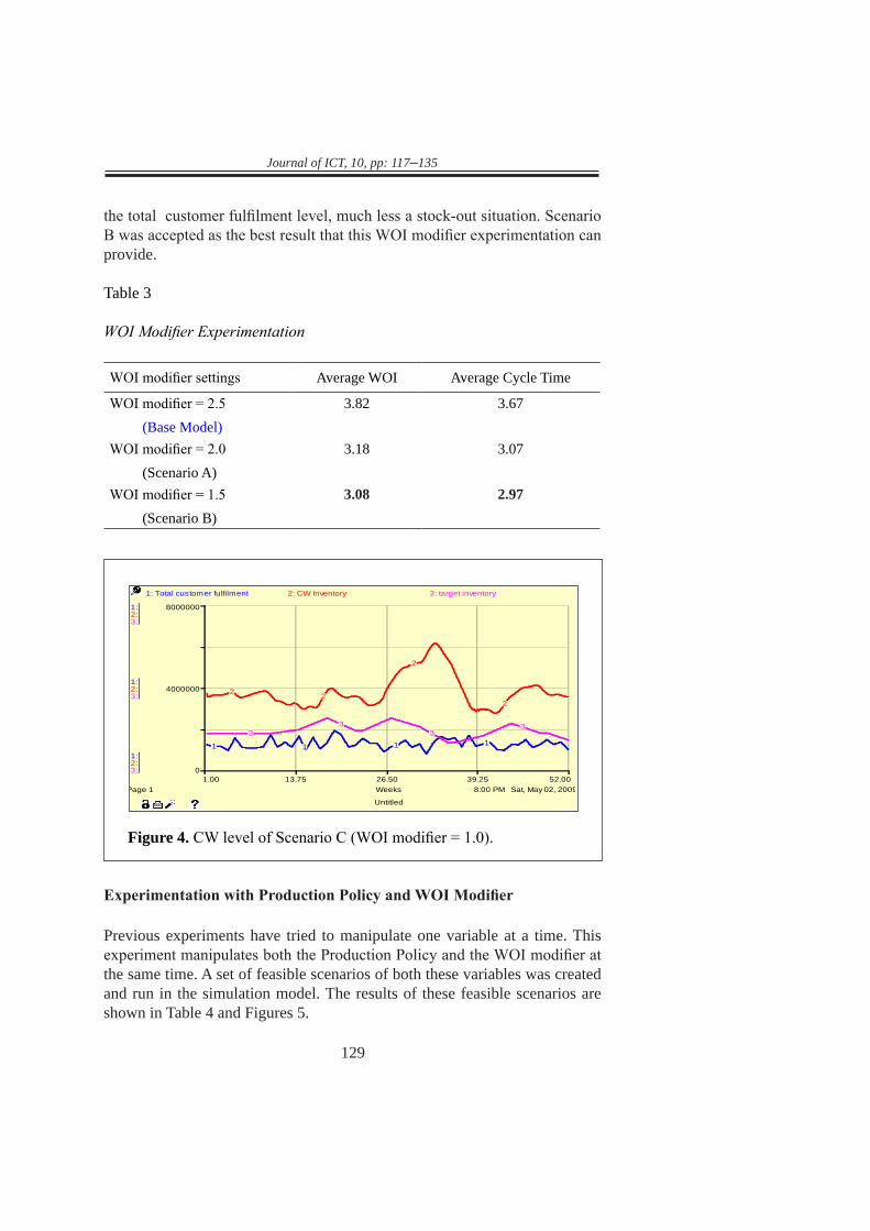
Table 3 shows that scenario B has the smallest value in terms of the average CW WOI level or the CW cycle time. This result appeared to be very good, as it is observed in Figure 4 that the CW Inventory level never went below

8:07 PM Sat, May 02, 2009

Untitled

Page 11.00 13.75 26.50 39.25 52.00

Weeks

1:

1:

1:

2:

2:

2:

3:

3:

3:

0

4000000

8000000

1: Total customer fulfilment 2: CW Inventory 3: target inventory

1 1 1 1

2

2

2

23

3

33

129


the total customer fulfilment level, much less a stock-out situation. Scenario B was accepted as the best result that this WOI modifier experimentation can provide.

Table 3

WOI Modifier Experimentation

WOI modifier settings Average WOI Average Cycle Time

WOI modifier = 2.5 3.82 3.67 (Base Model)WOI modifier = 2.0 3.18 3.07 (Scenario A)WOI modifier = 1.5 3.08 2.97 (Scenario B)

Figure 4. CW level of Scenario C (WOI modifier = 1.0).

Experimentation with Production Policy and WOI Modifier

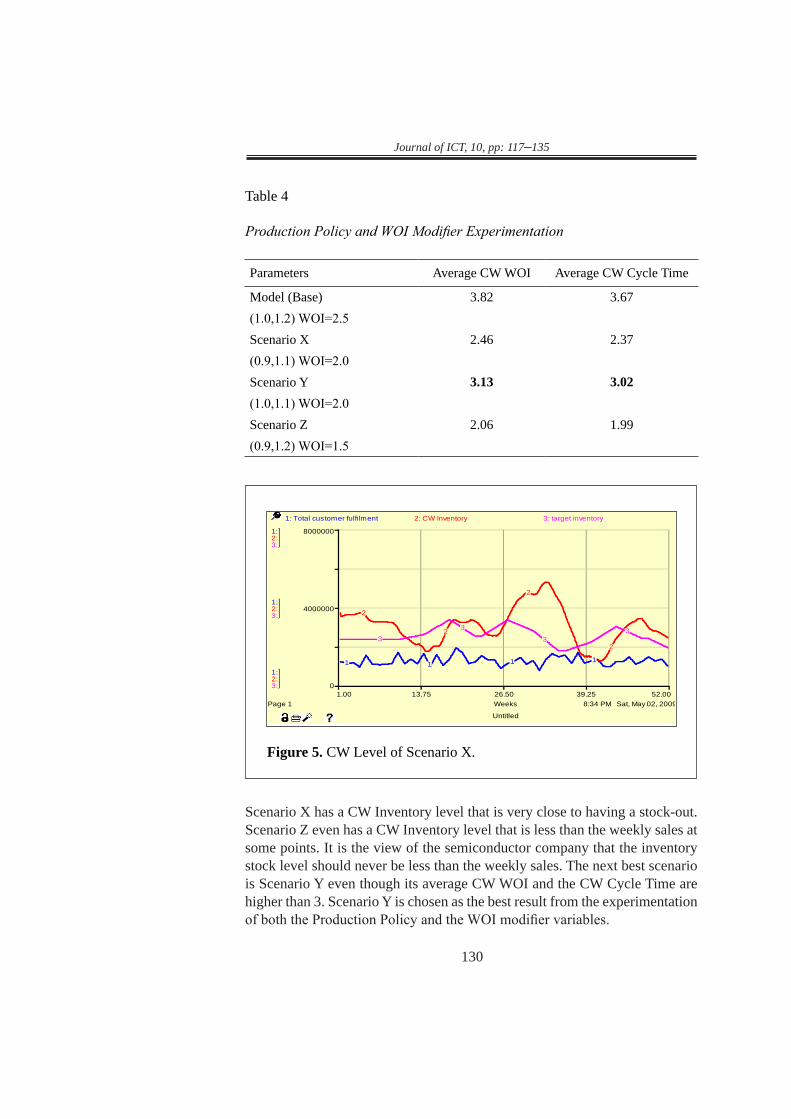
Previous experiments have tried to manipulate one variable at a time. This experiment manipulates both the Production Policy and the WOI modifier at the same time. A set of feasible scenarios of both these variables was created and run in the simulation model. The results of these feasible scenarios are shown in Table 4 and Figures 5.

8:00 PM Sat, May 02, 2009

Untitled

Page 11.00 13.75 26.50 39.25 52.00

Weeks

1:

1:

1:

2:

2:

2:

3:

3:

3:

0

4000000

8000000


1 1 1 1

22

2

2

33

33


130

Table 4

Production Policy and WOI Modifier Experimentation

Parameters Average CW WOI Average CW Cycle Time

Model (Base) 3.82 3.67(1.0,1.2) WOI=2.5Scenario X 2.46 2.37(0.9,1.1) WOI=2.0Scenario Y 3.13 3.02(1.0,1.1) WOI=2.0Scenario Z 2.06 1.99(0.9,1.2) WOI=1.5

Figure 5. CW Level of Scenario X.

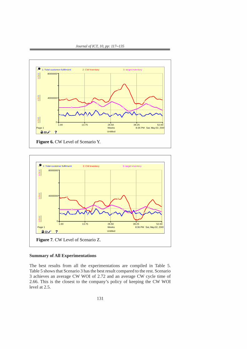
Scenario X has a CW Inventory level that is very close to having a stock-out. Scenario Z even has a CW Inventory level that is less than the weekly sales at some points. It is the view of the semiconductor company that the inventory stock level should never be less than the weekly sales. The next best scenario is Scenario Y even though its average CW WOI and the CW Cycle Time are higher than 3. Scenario Y is chosen as the best result from the experimentation of both the Production Policy and the WOI modifier variables.

8:34 PM Sat, May 02, 2009

Untitled

Page 11.00 13.75 26.50 39.25 52.00

Weeks

1:

1:

1:

2:

2:

2:

3:

3:

3:

0

4000000

8000000


1 1 1 1

2

2

2

23

3

33

131


Figure 6. CW Level of Scenario Y.

Figure 7. CW Level of Scenario Z.

Summary of All Experimentations

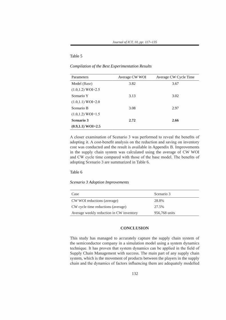
The best results from all the experimentations are compiled in Table 5. Table 5 shows that Scenario 3 has the best result compared to the rest. Scenario 3 achieves an average CW WOI of 2.72 and an average CW cycle time of 2.66. This is the closest to the company’s policy of keeping the CW WOI level at 2.5.

8:35 PM Sat, May 02, 2009

Untitled

Page 11.00 13.75 26.50 39.25 52.00

Weeks

1:

1:

1:

2:

2:

2:

3:

3:

3:

0

4000000

8000000


1 1 1 1

2 2

2

2

3

3

33

Figure 6. CW level of Scenario Y.

8:36 PM Sat, May 02, 2009

Untitled

Page 11.00 13.75 26.50 39.25 52.00

Weeks

1:

1:

1:

2:

2:

2:

3:

3:

3:

0

4000000

8000000


1 1 1 1

2

2

2

23

33

3

Figure 7. CW level of Scenario Z.


8:35 PM Sat, May 02, 2009

Untitled

Page 11.00 13.75 26.50 39.25 52.00

Weeks

1:

1:

1:

2:

2:

2:

3:

3:

3:

0

4000000

8000000


1 1 1 1

2 2

2

2

3

3

33

Figure 6. CW level of Scenario Y.

8:36 PM Sat, May 02, 2009

Untitled

Page 11.00 13.75 26.50 39.25 52.00

Weeks

1:

1:

1:

2:

2:

2:

3:

3:

3:

0

4000000

8000000


1 1 1 1

2

2

2

23

33

3

Figure 7. CW level of Scenario Z.



132

Table 5

Compilation of the Best Experimentation Results

Parameters Average CW WOI Average CW Cycle Time

Model (Base) 3.82 3.67(1.0,1.2) WOI=2.5

Scenario Y 3.13 3.02(1.0,1.1) WOI=2.0

Scenario B 3.08 2.97(1.0,1.2) WOI=1.5Scenario 3 2.72 2.66(0.9,1.1) WOI=2.5

A closer examination of Scenario 3 was performed to reveal the benefits of adopting it. A cost-benefit analysis on the reduction and saving on inventory cost was conducted and the result is available in Appendix B. Improvements in the supply chain system was calculated using the average of CW WOI and CW cycle time compared with those of the base model. The benefits of adopting Scenario 3 are summarized in Table 6.

Table 6

Scenario 3 Adoption Improvements

Case Scenario 3

CW WOI reductions (average) 28.8%CW cycle time reductions (average) 27.5%Average weekly reduction in CW inventory 956,768 units

CONCLUSION

This study has managed to accurately capture the supply chain system of the semiconductor company in a simulation model using a system dynamics technique. It has proven that system dynamics can be applied in the field of Supply Chain Management with success. The main part of any supply chain system, which is the movement of products between the players in the supply chain and the dynamics of factors influencing them are adequately modelled

133


in a simulation model. The model validation process supports that the model was able to capture the behaviour and the dynamics of the supply chain system quite successfully. This provides a platform for future studies into supply chain component’s relationship and power balance. This shows that the system dynamics approach to simulation modelling is capable of capturing the dynamics of the semiconductor company’s supply chain system.

The simulation model was also capable of assessing the policy and practices in the supply chain system. A simulation run can show observations and statistics on every part of the supply chain, which under the actual circumstances are difficult or impossible to perform. Companies with existing supply chain systems could refer to this research on how to better understand and visualize them. Given the ability to extract and manipulate information on any part of the supply chain system, alternative practices and what-if analysis can be performed on the simulation model without any risk or damage to the existing system. Experimentation of the simulation model has resulted in better policy settings that achieve an average saving of about one million units of inventory per week and an increase of efficiency of CW by reducing WOI by 28.8% and cycle time by 27.5%.

LIMITATIONS

This study has some limitations due to the nature of the data and the model structure. Firstly, actual data of Hubs and SFGI are input directly into the model. This means that their policies are not considered in the simulation model. This stabilizes the role of Hubs and SFGI in the simulated supply chain system but decreases its behaviour dynamics.

Secondly, the secondary data obtained from the database of the semiconductor company is at the family level of the product, not at the most detailed specifications level. This effectively eliminates the variations within the product lines. Product customizations are not accounted for and customer fulfilments are not thoroughly represented in the simulation model.

Finally, the product start-up period, called the ramp-up period, was not modelled into the simulation model. The ramp-up period happens in the first six months of the product life cycle. The volatile nature of a product start-up is not accounted for and its effects on the overall supply chain is ignored. The shortening of the simulation time period of one and a half years to one year reduces the overall comprehensiveness of the simulation model.


134

REFERENCES

An, L., & Jeng J. J. (2005). On developing system dynamics model for business process simulation. Proceedings of the 2005 Winter Simulation Conference.

Chow, W. S., Madu, C. N., Kuei, C. -H., Lu, M. H., Lin, C., & Tseng, H. (2006). Supply chain management in the US and Taiwan: An empirical study. Omega, 36(5), 665–679.

Christopher, M., & Lee, H. L. (2001). The key to effective supply chains through improved visibility and reliability. Global Trade Management, 1–0.

Eldabi, T., Irani, Z., Paul, R. J., & Love, P. E. D. (2002). Quantitative and qualitative decision-making methods in simulation modeling. Management Decision, 40(1), 64–3.

Ge, Y., Yang, J. -B., Proudlove, N., & Spring, M. (2004). System dynamics modeling for supply-chain management: A case study on a supermarket chain in the UK. International Transaction in Operation Research, 11, 495–509.

Greasly, A., & Barlow, S. (1998). Using simulation modeling for BPR: Resource allocation in a police custody process. International Journal of Operation and Production Management, 18(9/10), 978–988.

Inagaki, M., & Kuroda, K. (2007). Supply chain management in Japan. Supply & Demand Chain Executive, 8(3), 68.

Irani, Z., Hlupic, V., Baldwin, L. P., & Love, P. E. D. (2000). Re-engineering manufacturing processes through simulation modeling. Logistic Information Management, 13(1), 7–13

Kumar, S., & Yamaoka, T. (2007). System dynamics study of the Japanese automotive industry closed-loop supply chain. Journal Of Manufacturing Technology Management, 18(2), 115–138.

Kumar, V., Fantasy, K. A., & Kumar, U. (2006). Implementation and management framework for supply chain flexibility. Journal of Enterprise Information Management, 19(3), 303–319.

135


Levans, M. A. (2002). Bridging the supply chain and logistics cultural gap. Logistics Management, 46(6), 16.

Listl, A., & Notzon, I. (2000). An operational application of system dynamics in the automotive industry: Inventory management at BMW. International System Dynamic Conference, Bergen, Norway.

Lyneis, J. M. (1999). System dynamics for business strategy: A phased

approach. System Dynamics Review, 15(1), 37–70.

McDonagh, K. D. (2002). System dynamics simulation to improve harvesting system management (Unpublished master’s thesis). State University, Blacksburg, Virginia.

Mukherjee, A., & Roy, R. (2006). A system dynamic model of management of a television game show. Journal of Modeling Management, 1(2), 95–115.

Stevens, J. (1989). Integrating the supply chain. International Journal of Physical Distribution and Materials Management, 19(8), 3–8.

Sweetser, A. (1999). A comparison of System Dynamics (SD) and Discrete Event Simulation (DES). Paper presented at the System Dynamics Society and the 5th Australian & New Zealand Systems Conference, Wellington, New Zealand.

Taylor, D. A. (2004). Supply chains: A manager’s guide. Boston: Addison-Wesley.

Trkman, P., Stemberger, M. I., Jaklic, J., & Groznik, A. (2007). Process approach to supply chain integration. Supply Chain Management: An International Journal, 12(2), 116–128.

Vernadat, F. B. (1996). Enterprise modeling and integration – Principles and application. London: Chapman & Hall.

Documents

SUPPLY CHAIN MANAGEMENT: A SYSTEM DYNAMICS APPROACH …