Embed Size (px)
Citation preview

Supply Chain Networks, Electronic Commerce, and
Supply Side and Demand Side Risk
Anna Nagurney and Jose Cruz
Department of Finance and Operations Management
Isenberg School of Management
University of Massachusetts
and
June Dong and Ding Zhang
Department of Marketing and Management
School of Business
State University of New York at Oswego
Oswego, New York 13126
revised October, 2003; appears in European Journal of Operational Research (2005), 164, pp. 120-142.
Abstract: In this paper, we develop a supply chain network model in which both physical
and electronic transactions are allowed and in which supply side risk as well as demand side
risk are included in the formulation. The model consists of three tiers of decision-makers:
the manufacturers, the distributors, and the retailers, with the demands associated with
the retail outlets being random. We model the optimizing behavior of the various decision-
makers, with the manufacturers and the distributors being multicriteria decision-makers and
concerned with both profit maximization and risk minimization. We derive the equilibrium
conditions and establish the finite-dimensional variational inequality formulation. We pro-
vide qualitative properties of the equilibrium pattern in terms of existence and uniqueness
results and also establish conditions under which the proposed computational procedure
is guaranteed to converge. We illustrate the supply chain network model through several
numerical examples for which the equilibrium prices and product shipments are computed.
This is the first multitiered supply chain network equilibrium model with electronic com-
merce and with supply side and demand side risk for which modeling, qualitative analysis,
and computational results have been obtained.
Key Words: Supply chains; Networks; Electronic commerce; Risk management; Multicri-
teria optimization; Network equilibrium; Variational inequalities
1

1. Introduction
Supply chain networks have evolved to become critical structures in the production and
dissemination of goods in today’s modern economies. Since they involve manufacturers,
distributors, retailers, as well as consumers, which are spatially dispersed, they must respond
to the realities of world events, which, in the given age, are characterized by heightened risks
and uncertainty. Furthermore, the management of supply chain networks must consider
the complexity of interactions among the various decision-makers, coupled with appropriate
decision-making criteria, in this new world order.
Given the importance of supply chain networks in practice, there has been increased
attention focused on disruptions to supply chains from various directions. Threats to the
optimal functioning of supply chains have included both human disruptions (cf. Sheffi (2001))
as well as biological ones, including, for example, the SARS virus (see Engardio et al. (2003)).
Such realities have brought even greater pressure and need for the rigorous formulation and
analysis of supply chain networks.
On the positive side, advances in electronic commerce have unveiled new opportunities for
the management of supply chain networks (cf. Nagurney and Dong (2002) and the references
therein). Notably, electronic commerce (e-commerce) has had an immense effect on the
manner in which businesses order goods and have them transported with the major portion
of e-commerce transactions being in the form of business-to-business (B2B). Estimates of
B2B electronic commerce range from approximately .1 trillion dollars to 1 trillion dollars in
1998 and with forecasts reaching as high as $4.8 trillion dollars in 2003 in the United States
(see Federal Highway Administration (2000), Southworth (2000)). Moreover, according to
the National Research Council (2000), the principal effect of business-to-business (B2B)
commerce, estimated to be 90% of all electronic commerce by value and volume, is in the
creation of new and more profitable supply chain networks.
Furthermore, the availability of electronic commerce in which the physical ordering of
goods (and supplies) (and, is some cases, even delivery) is replaced by electronic orders,
offers the potential of reducing risks associated with physical transportation due to potential
threats and disruptions as mentioned above.
2

In this paper, we take upon the challenge of formalizing decision-making in multitiered
supply chain networks in a scenario of risk and uncertainty. Our motivation comes from
practice but the approach is technical and rigorous. Our framework builds upon the recent
advances in supply chain network equilibrium modeling in the case of random demands
without and with electronic commerce, respectively (cf. Dong, Zhang, and Nagurney (2002a,
2003)) and with multicriteria decision-makers (cf. Dong, Zhang, and Nagurney (2002b) and
Dong et al. (2003)). Here, however, and unlike the preceding papers, we are explicitly
concerned with risk management on the supply side in terms of the manufacturers and
the distributors. In addition, we retain the measurement of demand side risk. The need to
incorporate both supply and demand side risks is well-documented in the literature (see, e.g.,
Smeltzer and Siferd (1998), Agrawal and Seshadri (2000), Johnson (2001), Zsidisin (2003)).
For additional recent research on supply chains including electronic commerce, see the edited
volumes by Geunes, Pardalos, and Romeijn (2002) and by Pardalos and Tsitsiringos (2002).
Our focus in this paper is to also provide the foundations upon which a global supply
chain network model can be built that captures both supply side and demand side risk. Some
preliminary results can be found in Nagurney, Cruz, and Matsypura (2003). Frameworks
for risk management in a global supply chain context with a focus on centralized decision-
making and optimization can be found in Huchzermeier and Cohen (1996), Cohen and Mallik
(1997), and the references therein.
The paper is organized as follows. In Section 2, we develop the supply chain network
model with decentralized decision-makers and with supply side and demand side risk. We
derive the optimality conditions of the various decision-makers, and establish that the govern-
ing equilibrium conditions can be formulated as a finite-dimensional variational inequality
problem. We emphasize here that the concept of equilibrium, first explored in a general
setting for supply chains by Nagurney, Dong, and Zhang (2002) (see also Nagurney et al.
(2002)), provides a valuable benchmark against which prices of the product at the various
tiers of the network as well as product flows between tiers can be compared.
In Section 3, we study qualitative properties of the equilibrium pattern, and, under rea-
sonable conditions, establish existence and uniqueness results. We also provide properties
of the function that enters the variational inequality that allows us to establish convergence
3

of the proposed algorithmic scheme in Section 4. In Section 5, we apply the algorithm to
several supply chain network examples for the computation of the equilibrium prices and
shipments. The paper concludes with Section 6, in which we summarize our results and
present suggestions for future research.
4

2. The Supply Chain Network Equilibrium Model with Supply Side and Demand
Side Risk
In this section, we develop the supply chain network model. The multicriteria decision-
makers on the supply side in the form of manufacturers and distributors are concerned not
only with profit maximization but also with risk minimization. The demand side risk, in
turn, is represented by the uncertainty surrounding the random demands at the retailers.
The model allows for not only physical transactions but also electronic transactions.
In particular, we consider m manufacturers involved in the production of a homogeneous
product which is then shipped to n distributors, who, in turn, ship the product to o retailers.
The retailers can transact either physically (in the standard manner) with the distributors or
directly, in an electronic manner, with the manufacturers (see also Nagurney et al. (2002)).
We denote a typical manufacturer by i, a typical distributor by j, and a typical retailer
by k. Note that (cf. Figure 1) the manufacturers are located at the top tier of nodes of the
network, the distributors at the middle tier, and the retailers at the third or bottom tier
of nodes. The links in the supply chain supernetwork (cf. Nagurney and Dong (2002)) in
Figure 1 include classical physical links as well as Internet links to allow for e-commerce.
The introduction of e-commerce allows for “connections” that were, heretofore, not possi-
ble, such as, for example, those enabling retailers to purchase a product directly from the
manufacturers.
The behavior of the various network decision-makers represented by the three tiers of
nodes in Figure 1 is now described. We first focus on the manufacturers. We then turn
to the distributors, and, subsequently, to the retailers. Both the manufacturers and the
distributors are assumed to be multicriteria decision-makers and are concerned not only
with profit maximization but also with risk minimization.
The Behavior of the Manufacturers and their Optimality Conditions
Let qi denote the nonnegative production output of manufacturer i. Group the production
outputs of all manufacturers into the column vector q ∈ Rm+ . Here it is assumed that each
manufacturer i is faced with a production cost function fi, which can depend, in general, on
5

InternetLink
����1 ����
· · · j · · · ����n Distributors
����1 ����
· · · i · · · ����m
Physical Links
����1 ����
· · · k · · · ����o
?
@@
@@
@@R
PPPPPPPPPPPPPPPPq
��
��
�� ?
HHHHHHHHHHHj
���������������������9
����������������)
��
��
��
?
@@
@@
@@R
XXXXXXXXXXXXXXXXXXXXXz
��
��
�� ?
PPPPPPPPPPPPPPPPq
����������������)
������������
@@
@@
@@R
InternetLink
InternetLink
· · · Physical
Link
Manufacturers
Retailers
Figure 1: The Supernetwork Structure of the Supply Chain
the entire vector of production outputs, that is,
fi = fi(q), ∀i. (1)
Hence, the production cost of a particular manufacturer can depend not only on his pro-
duction output but also on those of the other manufacturers. This allows one to model
competition.
The transaction cost associated with manufacturer i transacting with distributor j is
denoted by cij. The product shipment between manufacturer i and distributor j is denoted by
qij. The product shipments between all pairs of manufacturers and distributors are grouped
into the column vector Q1 ∈ Rmn+ . In addition, a manufacturer i may transact directly
with the retailer k with this transaction cost associated with the Internet transaction begin
denoted by cik and the associated product shipment from manufacturer i to retailer k by qik.
We group these product shipments into the column vector Q2 ∈ Rmo+ .
The transaction cost between a manufacturer and distributor pair and the transaction cost
between a manufacturer and retailer may depend upon the volume of transactions between
6

each such pair, and are given, respectively, by:
cij = cij(qij), ∀i, j, (2a)
and
cik = cik(qik), ∀i, k. (2b)
The quantity produced by manufacturer i must satisfy the following conservation of flow
equation:
qi =n∑
j=1
qij +o∑
k=1
qik, (3)
which states that the quantity produced by manufacturer i is equal to the sum of the quan-
tities shipped from the manufacturer to all distributors and to all retailers.
The total costs incurred by a manufacturer i, thus, are equal to the sum of the man-
ufacturer’s production cost plus the total transaction costs. His revenue, in turn, is equal
to the price that the manufacturer charges for the product times the total quantity ob-
tained/purchased of the product from the manufacturer by all the distributors and all the
retailers. Let ρ∗1ij denote the price charged for the product by manufacturer i to distributor j
who has transacted, and let ρ∗1ik denote the price charged by manufacturer i for the product
to the retailer k. Hence, manufacturers can price according to their locations, as to whether
the product is sold to the distributor or to the retailers directly, and according to whether
the transaction was conducted via the Internet or not. How these prices are arrived at is
discussed later in this section.
Noting the conservation of flow equations (3) and the production cost functions (1), one
can express the criterion of profit maximization for manufacturer i as:
Maximizen∑
j=1
ρ∗1ijqij +
o∑
k=1
ρ∗1ikqik − fi(Q
1, Q2) −n∑
j=1
cij(qij) −o∑
k=1
cik(qik), (4)
subject to qij ≥ 0, for all j, and qik ≥ 0, for all k.
Note that the first two terms in (4) correspond to the revenue whereas the subsequent
three terms denote the production cost and the transaction costs, respectively.
7

In addition to the criterion of profit mazimization we also assume that each manufacturer
is concerned with risk minimization. Here, for the sake of generality, we assume, as given,
a risk function ri, for manufacturer i, which is assumed to be continuous and convex and a
function of not only the shipments associated with the manufacturer but also of the shipments
of other manufacturers. Hence, we assume that
ri = ri(Q1, Q2), ∀i. (5)
Note that according to (5) the risk as perceived by a manufacturer is dependent not only
upon the flows that he controls but also on those controlled by others. Hence, the second
criterion of manufacturer i can be expressed as:
Minimize ri(Q1, Q2), (6)
subject to: qij ≥ 0, ∀j and qik ≥ 0, ∀k.
Each manufacturer i associates a nonnegative weight αi with the risk minimization crite-
rion (6), with the weight associated with the profit maximization criterion (4) serving as the
numeraire and being set equal to 1. Hence, we can construct a value function for each man-
ufacturer (cf. Fishburn (1970), Chankong and Haimes (1983), Yu (1985), Keeney and Raiffa
(1993)) using a constant additive weight value function. Consequently, the multicriteria
decision-making problem for manufacturer i is transformed into:
Maximizen∑
j=1
ρ∗1ijqij +
o∑
k=1
ρ∗1ikqik −fi(Q
1, Q2)−n∑
j=1
cij(qij)−o∑
k=1
cij(qik)−αiri(Q1, Q2), (7)
subject to: qij ≥ 0, ∀j; qik ≥ 0, ∀k.
The manufacturers are assumed to compete in a noncooperative fashion. Also, it is
assumed that the production cost functions and the transaction cost functions for each
manufacturer are continuous and convex. The governing optimization/equilibrium concept
underlying noncooperative behavior is that of Nash (1950, 1951), which states, in this con-
text, that each manufacturer will determine his optimal production quantity and shipments,
given the optimal ones of the competitors. Hence, the optimality conditions for all manu-
facturers simultaneously can be expressed as the following inequality (see also Gabay and
8

Moulin (1980), Bazaraa, Sherali, and Shetty (1993), Nagurney (1999), Nagurney, Dong, and
Zhang (2002)): determine the solution (Q1∗, Q2∗) ∈ Rmn+mo+ , which satisfies:
m∑
i=1
n∑
j=1
[∂fi(Q
1∗, Q2∗)
∂qij+
∂cij(q∗ij)
∂qij+ αi
∂ri(Q1∗, Q2∗)
∂qij− ρ∗
1ij
]×[qij − q∗ij
]
+m∑
i=1
o∑
k=1
[∂fi(Q
1∗, Q2∗)
∂qik+
∂cik(q∗ik)
∂qik+ αi
∂ri(Q1∗, Q2∗)
∂qik− ρ∗
1ik
]× [qik − q∗ik] ≥ 0, (8)
∀(Q1, Q2) ∈ Rmn+mo+ .
The inequality (8), which is a variational inequality has a nice economic interpretation. In
particular, from the first term one can infer that, if there is a positive shipment of the product
transacted between manufacturer and a distributor, then the marginal cost of production
plus the marginal cost of transacting plus the weighted marginal risk associated with that
transaction must be equal to the price that the distributor is willing to pay for the product.
If the marginal cost of production plus the marginal cost and weighted marginal risk of
transacting exceeds that price, then there will be zero volume of flow of the product between
the two. The second term in (8) has a similar interpretation; in particular, there will be a
positive volume of flow of the product from a manufacturer to a retailer if the marginal cost
of production of the manufacturer plus the marginal cost of transacting with the retailer via
the Internet and the weighted marginal risk is equal to the price the retailers are willing to
pay for the product.
Note that in the above framework we explicitly allow each of the decision-makers, in
the form of manufacturers, to not only have distinct risk functions but also distinct weights
associated with their respective weight functions. We emphasize that the study of risk has
had a long and prominent history in the field of finance, dating to the work of Markowitz
(1952, 1959), whereas the incorporation of risk into supply chain management has only been
addressed fairly recently. Furthermore, we emphasize that by allowing the risk function to
be general one can then construct an appropriate function pertaining to the specific situation
and decision-maker. For example, in the field of finance, measurement of risk has included the
use of variance-covariance matrices, yielding quadratic expressions for the risk (see also, e.g.,
Nagurney and Siokos (1997)). In addition, in finance, the bicriteria optimization problem of
9

net revenue maximization and risk minimization is fairly standard (see also, e.g., Dong and
Nagurney (2001)).
The Behavior of the Distributors and their Optimality Conditions
The distributors, in turn, are involved in transactions both with the manufacturers as
well as with the retailers. Let qjk denote the amount of the product purchased by retailer k
from distributor j. Group these shipment quantities into the column vector Q3 ∈ Rno+ .
A distributor j is faced with what is termed a handling cost, which may include, for
example, the loading/unloading and storage costs associated with the product. Denote this
cost by cj and, in the simplest case, one would have that cj is a function of∑m
i=1 qij and∑o
k=1 qjk that is, the inventory cost of a distributor is a function of how much of the product
he has obtained from the various manufacturers and how much of the product he has shipped
out to the various retailers. However, for the sake of generality, and to enhance the modeling
of competition, allow the function to, in general, depend also on the amounts of the product
held by other distributors. Therefore, one may write:
cj = cj(Q1, Q3), ∀j. (9)
Distributor j associates a price with the product, which is denoted by γ∗j . This price,
as will be shown, will also be endogenously determined in the model and will be, given a
positive volume of flow between a distributor and any retailer, related to a clearing-type
price. Assuming that the distributors are also profit-maximizers, the optimization problem
of a distributor j is given by:
Maximize γ∗j
o∑
k=1
qjk − cj(Q1, Q3) −
m∑
i=1
ρ∗1ijqij (10)
subject to:o∑
k=1
qjk ≤m∑
i=1
qij, (11)
and the nonnegativity constraints: qij ≥ 0, and qjk ≥ 0, for all i, and k. Objective function
(10) expresses that the difference between the revenues and the handling cost and the payout
to the manufacturers should be maximized. Constraint (11) expresses that the retailers
cannot purchase more from a distributor than is held in stock.
10

In addition, each distributor seeks to also minimze his risk associated with obtaining and
shipping the product to the various retailers. We assume that each distributor j is faced
with his own individual risk denoted by rj with the function being assumed to be continuous
and convex and dependent on the shipments to and from all the distributors, that is,
rj = rj(Q1, Q3), ∀j. (12)
The model assumes that each distributor associates a weight of 1 with the profit criterion
(10) and a weight of βj to his risk level. Therefore, the multicriteria decision-making problem
for distributor j; j = 1, . . . , n, can be transformed directly into the optimization problem:
Maximize γ∗j
o∑
k=1
qjk − cj(Q1, Q3) −
m∑
i=1
ρ∗1ijqij − βjrj(Q
1, Q3) (13)
subject to:o∑
k=1
qjk ≤m∑
i=1
qij, (14)
and the nonnegativity constraints: qij ≥ 0, and qjk ≥ 0, for all i and k.
Objective function (13) represents a value function for distributor j with βj having the
interpretation as a conversion rate in dollar value.
The optimality conditions of the distributors are now obtained, assuming that each dis-
tributor is faced with the optimization problem (13), subject to (14), and the nonnegativity
assumption on the variables.
Here it is also assumed that the distributors compete in a noncooperative manner, given
the actions of the other distributors. Note that, at this point, we consider that distributors
seek to determine not only the optimal amounts purchased by the retailers, but, also, the
amount that they wish to obtain from the manufacturers. In equilibrium, all the shipments
between the tiers of network decision-makers will have to coincide.
Assuming that the handling cost for each distributor is continuous and convex as are the
transaction costs, the optimal (Q1∗, Q3∗, ρ∗2) ∈ Rmn+no+n
+ satisfy the optimality conditions
for all the distributors or, equivalently, the variational inequality:m∑
i=1
n∑
j=1
[∂cj(Q
1∗, Q3∗)
∂qij+ ρ∗
1ij + βj∂rj(Q
1∗, Q3∗)
∂qij− ρ∗
2j
]×[qij − q∗ij
]
11

+n∑
j=1
o∑
k=1
[−γ∗
j +∂cj(Q
1∗, Q3∗)
∂qjk+ ρ∗
2j + βj∂rj(Q
1∗, Q3∗)
∂qjk
]×[qjk − q∗jk
]
+n∑
j=1
[m∑
i=1
q∗ij −o∑
k=1
q∗jk
]×[ρ2j − ρ∗
2j
]≥ 0, ∀Q1 ∈ Rmn
+ , ∀Q3 ∈ Rno+ , ∀ρ2 ∈ Rn
+, (15)
where ρ2j is the Lagrange multiplier associated with constraint (14) for distributor j and ρ2 is
the column vector of all the distributors’ multipliers. In this derivation, as in the derivation
of inequality (8), the prices charged were not variables. The γ∗ = (γ∗1 , . . . , γ
∗n) is the vector
of endogenous equilibrium prices in the complete model.
The economic interpretation of the distributors’ optimality conditions is now highlighted.
From the second term in inequality (15), one has that, if retailer k purchases the product
from a distributor j, that is, if the q∗jk is positive, then the price charged by retailer j, γ∗j , is
equal to the marginal handling cost and the weighted marginal risk, plus the shadow price
term ρ∗2j, which, from the third term in the inequality, serves as the price to clear the market
from distributor j. Furthermore, from the first term in inequality (15), one can infer that, if a
manufacturer transacts with a distributor resulting in a positive flow of the product between
the two, then the price ρ∗2j is precisely equal to distributor j’s payment to the manufacturer,
ρ∗1ij, plus his marginal cost of handling the product associated with transacting with the
particular manufacturer plus the weighted marginal risk associated with the transaction.
In the above derivations, we have considered supply side risk from the perspective of the
manufacturers as well as the distributors. We now turn to the retailers and consider demand
side risk which is modeled in a stochastic manner to represent the uncertainty. Clearly,
if the demands were known with certainty there would be no risk associated with them
and the retailers and manufacturers could make their production and distribution decisions
accordingly.
The Retailers and their Optimality Conditions
The retailers, in turn, must decide how much to order from the distributors and from the
manufacturers in order to cope with the random demand while still seeking to maximize their
profits. A retailer k is also faced with what we term a handling cost, which may include, for
example, the display and storage cost associated with the product. We denote this cost by
12

ck and, in the simplest case, we would have that ck is a function of sk =∑m
i=1 qik +∑n
j=1 qjk,
that is, the holding cost of a retailer is a function of how much of the product he has
obtained from the various manufacturers directly through orders via the Internet and from
the various distributors. However, for the sake of generality, and to enhance the modeling of
competition, we allow the function to, in general, depend also on the amounts of the product
held by other retailers and, therefore, we may write:
ck = ck(Q2, Q3), ∀k. (16)
Let ρ3k denote the demand price of the product associated with retailer k. We assume
that d̂k(ρ3k) is the demand for the product at the demand price of ρ3k at retail outlet k,
where d̂k(ρ3k) is a random variable with a density function of Fk(x, ρ3k), with ρ3k serving as
a parameter. Hence, we assume that the density function may vary with the demand price.
Let Pk be the probability distribution function of d̂k(ρ3k), that is, Pk(x, ρ3k) = Pk(d̂k ≤ x) =∫ x0 Fk(x, ρ3k)dx.
Retailer k can sell to the consumers no more than the minimum of his supply or his
demand, that is, the actual sale of k cannot exceed min{sk, d̂k}. Let
∆+k ≡ max{0, sk − d̂k} (17)
and
∆−k ≡ max{0, d̂k − sk}, (18)
where ∆+k is a random variable representing the excess supply (inventory), whereas ∆−
k is a
random variable representing the excess demand (shortage).
Note that the expected values of excess supply and excess demand of retailer k are scalar
functions of sk and ρ3k. In particular, let e+k and e−k denote, respectively, the expected values:
E(∆+k ) and E(∆−
k ), that is,
e+k (sk, ρ3k) ≡ E(∆+
k ) =∫ sk
0(sk − x)Fk(x, ρ3k)dx, (19)
e−k (sk, ρ3k) ≡ E(∆−k ) =
∫ ∞
sk
(x − sk)Fk(x, ρ3k)dx. (20)
13

Assume that the unit penalty of having excess supply at retail outlet k is λ+k and that
the unit penalty of having excess demand is λ−k , where the λ+
k and the λ−k are assumed to
be nonnegative. Then, the expected total penalty of retailer k is given by
E(λ+k ∆+
k + λ−k ∆−
k ) = λ+k e+
k (sk, ρ3k) + λ−k e−k (sk, ρ3k).
Assuming, as already mentioned, that the retailers are also profit-maximizers, the ex-
pected revenue of retailer k is E(ρ3k min{sk, d̂k}). Hence, the optimization problem of a
retailer k can be expressed as:
Maximize E(ρ3k min{sk, d̂k})−E(λ+k ∆+
k + λ−k ∆−
k )− ck(Q2, Q3)−
m∑
i=1
ρ∗1ikqik −
n∑
j=1
γ∗j qjk (21)
subject to:
qik ≥ 0, qjk ≥ 0, for all i and j. (22)
Objective function (21) expresses that the expected profit of retailer k, which is the
difference between the expected revenues and the sum of the expected penalty, the handling
cost, and the payouts to the manufacturers and to the distributors, should be maximized.
Applying now the definitions of ∆+k , and ∆−
k , we know that min{sk, d̂k} = d̂k − ∆−k .
Therefore, the objective function (21) can be expressed as
Maximize ρ3kdk(ρ3k)−(ρ3k+λ−k )e−k (sk, ρ3k)−λ+
k e+k (sk, ρ3k)−ck(Q
2, Q3)−m∑
i=1
ρ∗1ikqik−
n∑
j=1
γ∗j qjk
(23)
where dj(ρ3k) ≡ E(d̂k) is a scalar function of ρ3k.
We now consider the optimality conditions of the retailers assuming that each retailer
is faced with the optimization problem (21), subject to (22), which represents the nonneg-
ativity assumption on the variables. Here, we also assume that the retailers compete in a
noncooperative manner so that each maximizes his profits, given the actions of the other
retailers. Note that, at this point, we consider that retailers seek to determine the amount
that they wish to obtain from the manufacturers and from the distributors. First, however,
we make the following derivation and introduce the necessary notation:
∂e+k (sk, ρ3k)
∂qik=
∂e+k (sk, ρ3k)
∂qjk= Pk(sk, ρ3k) = Pk(
m∑
i=1
qik +n∑
j=1
qjk, ρ3k) (24)
14
∂e−k (sk, ρ3k)
∂qik=
∂e−k (sk, ρ3k)
∂qjk= Pk(sk, ρ3k) − 1 = Pk(
m∑
i=1
qij +n∑
j=1
qjk, ρ3k) − 1. (25)
Assuming that the handling cost for each retailer is continuous and convex, then the opti-
mality conditions for all the retailers satisfy the variational inequality: determine (Q2∗, Q3∗) ∈Rmo+no
+ , satisfying:
m∑
i=1
o∑
k=1
[λ+
k Pk(s∗k, ρ3k) − (λ−
k + ρ3k)(1 − Pk(s∗k, ρ3k)) +
∂ck(Q2∗, Q3∗)
∂qik+ ρ∗
1ik
]× [qik − q∗ik]
+n∑
j=1
o∑
k=1
[λ+
k Pk(s∗k, ρ3k) − (λ−
k + ρ3k)(1 − Pk(s∗k, ρ3k)) +
∂ck(Q2∗, Q3∗)
∂qjk
+ γ∗j
]×[qjk − q∗jk
]≥ 0,
∀(Q2, Q3) ∈ Rmo+no+ . (26)
In this derivation, as in the derivation of inequalities (8) and (15), we have not had the
prices charged be variables. They become endogenous variables in the complete supply chain
network model. A similar derivation but in the absence of electronic commerce (and in the
case of only a two-tiered rather than a three-tiered supply chain network) was obtained in
Dong, Zhang, and Nagurney (2002a).
We now highlight the economic interpretation of the retailers’ optimality conditions. In
inequality (26), we can infer that, if a manufacturer i transacts with a retailer k resulting
in a positive flow of the product between the two, then the selling price at retail outlet k,
ρ3k, with the probability of (1 − Pk(∑m
i=1 q∗ik +∑n
j=1 q∗jk, ρ3k)), that is, when the demand is
not less then the total order quantity, is precisely equal to the retailer k’s payment to the
manufacturer, ρ∗1ik, plus his marginal cost of handling the product and the penalty of having
excess demand with probability of Pk(∑m
i=1 q∗ik+∑o
j=1 q∗jk, ρ3k), (which is the probability when
actual demand is less than the order quantity), subtracted by the penalty of having shortage
with probability of (1−Pk(∑m
i=1 q∗ik +∑o
j=1 q∗jk, ρ3k)) (when the actual demand is greater than
the order quantity).
Similarly, if a distributor j transacts with a retailer k resulting in a positive flow of the
product between the two, then the selling price at retail outlet k, ρ3k, with the probability
of (1 − Pk(∑m
i=1 q∗ik +∑n
j=1 q∗jk, ρ3k)), that is, when the demand is not less then the total
15

order quantity, is precisely equal to the retailer k’s payment to the manufacturer, γ∗j , plus
his marginal cost of handling the product and the penalty of having excess demand with
probability of Pk(∑m
i=1 q∗ik +∑o
j=1 q∗jk, ρ3k), (which is the probability when actual demand is
less than the order quantity), subtracted by the penalty of having shortage with probability
of (1 − Pk(∑m
i=1 q∗ik +∑o
j=1 q∗jk, ρ3k)) (when the actual demand is greater than the order
quantity).
The Equilibrium Conditions
We now turn to a discussion of the market equilibrium conditions. Subsequently, we
construct the equilibrium conditions for the entire supply chain network.
The equilibrium conditions associated with the transactions that take place between the
retailers and the consumers are the stochastic economic equilibrium conditions, which, math-
ematically, take on the following form: For any retailer k; k = 1, . . . , o:
d̂k(ρ∗3k)
{≤ ∑m
i=1 q∗ik +∑o
j=1 q∗jk a.e., if ρ∗3k = 0
=∑m
i=1 q∗ik +∑o
j=1 q∗jk a.e., if ρ∗3k > 0,
(27)
where a.e. means that the corresponding equality or inequality holds almost everywhere.
Conditions (27) state that, if the demand price at outlet k is positive, then the quantities
purchased by the retailer from the manufacturers and from the distributors in the aggregate
is equal to the demand, with exceptions of zero probability. These conditions correspond
to the well-known economic equilibrium conditions (cf. Nagurney (1999) and the references
therein). Related equilibrium conditions, but without electronic transactions allowed, were
proposed in Dong, Zhang, and Nagurney (2002a).
Equilibrium conditions (27) are equivalent to the following variational inequality prob-
lem, after taking the expected value and summing over all retailers k: determine ρ∗3 ∈ Ro
+
satisfying
o∑
k=1
(m∑
i=1
q∗ik +n∑
j=1
q∗jk − dk(ρ∗3k)) × [ρ3k − ρ∗
3k] ≥ 0, ∀ρ3 ∈ Ro+, (28)
where ρ3 is the o-dimensional column vector with components: {ρ31, . . . , ρ3o}.
16

The Equilibrium Conditions of the Supply Chain
In equilibrium, we must have that the sum of the optimality conditions for all manu-
facturers, as expressed by inequality (8), the optimality conditions of the distributors, as
expressed by condition (15), the optimality conditions for all retailers, as expressed by in-
equality (26), and the market equilibrium conditions, as expressed by inequality (28) must be
satisfied. Hence, the shipments that the manufacturers ship to the retailers must be equal to
the shipments that the retailers accept from the manufacturers. In addition, the shipments
shipped from the manufacturers to the distributors, must be equal to those accepted by the
distributors, and, finally, the shipments from the distributors to the retailers must coincide
with those accepted by the retailers. We state this explicitly in the following definition:
Definition 1: Supply Chain Network Equilibrium with Supply Side and Demand
Side Risk
The equilibrium state of the supply chain network with supply and demand side risk is one
where the product flows between the tiers of the decision-makers coincide and the product
shipments and prices satisfy the sum of the optimality conditions (8), (15), and (26), and
the conditions (28).
The summation of inequalities (8), (15), (26), and (28) (with the prices at the manu-
facturers, the distributors, and at the retailers denoted, respectively, by their values at the
equilibrium, and denoted by ρ∗1, ρ∗
2, and ρ∗3), after algebraic simplification, yields the following
result:
Theorem 1: Variational Inequality Formulation
A product shipment and price pattern (Q1∗, Q2∗, Q3∗, ρ∗2, ρ
∗3)∈K is an equilibrium pattern of
the supply chain model according to Definition 1 if and only if it satisfies the variational
inequality problem:
m∑
i=1
n∑
j=1
[∂fi(Q
1∗, Q2∗)
∂qij+
∂cij(q∗ij)
∂qij+
∂cj(Q1∗, Q3∗)
∂qij+ αi
∂ri(Q1∗, Q2∗)
∂qij+ βj
∂rj(Q1∗, Q3∗)
∂qij− ρ∗
2j
]
×[qij − q∗ij
]+
m∑
i=1
o∑
k=1
[∂fi(Q
1∗, Q2∗)
∂qik
+∂cik(q
∗ik)
∂qik
+∂ck(Q
2∗, Q3∗)
∂qik
+ αi∂ri(Q
1∗, Q2∗)
∂qik
17

+λ+k Pk(s
∗k, ρ
∗3k) − (λ−
k + ρ∗3k)(1 − Pk(s
∗k, ρ
∗3k))
]× [qik − q∗ik]
+n∑
j=1
o∑
k=1
[λ+
k Pk(s∗k, ρ
∗3k) − (λ−
k + ρ∗3k)(1 − Pk(s
∗k, ρ
∗3k)) +
∂cj(Q1∗, Q3∗)
∂qjk
+∂ck(Q
2∗, Q3∗)
∂qjk
+ βj∂rj(Q
1∗, Q3∗)
∂qjk
+ ρ∗2j
]×[qjk − q∗jk
]+
n∑
j=1
[m∑
i=1
q∗ij −o∑
k=1
q∗jk
]×[ρ2j − ρ∗
2j
]
+o∑
k=1
n∑
j=1
q∗jk +m∑
i=1
q∗ik − dk(ρ∗3)
× [ρ3k − ρ∗
3k] ≥ 0, ∀(Q1, Q2, Q3, ρ2, ρ3) ∈ K, (29)
where K ≡ {(Q1, Q2, Q3, ρ2, ρ3)|(Q1, Q2, Q3, ρ2, ρ3) ∈ Rmn+mo+no+n+o+ }.
For easy reference in the subsequent sections, variational inequality problem (29) can be
rewritten in standard variational inequality form (cf. Nagurney (1999)) as follows: Determine
X∗ ∈ K satisfying:
〈F (X∗), X − X∗〉 ≥ 0, ∀X ∈ K ≡ Rmn+mo+no+n+o+ , (30)
where X ≡ (Q1, Q2, Q3, ρ2, ρ3), F (X) ≡ (Fij, Fik, Fjk, Fj, Fk)i=1,...,m;j=1,...,n;k=1,...,o, and the
specific components of F are given by the functional terms preceding the multiplication
signs in (29). The term 〈·, ·〉 denotes the inner product in N -dimensional Euclidean space.
Note that the variables in the model (and which can be determined from the solution of
either variational inequality (29) or (30)) are: the equilibrium product shipments between
manufacturers and the distributors given by Q1∗, the equilibrium product shipments trans-
acted electronically between the manufacturers and the retailers denoted by Q2∗, and the
equilibrium product shipments between the distributors and the retailers given by Q3∗, as
well as the equilibrium demand prices ρ∗3 and the equilibrium prices ρ∗
2. We now discuss how
to recover the prices ρ∗1 associated with the top tier of nodes of the supply chain supernetwork
and the prices γ∗ associated with the middle tier.
First note that from (8), we have that (as already discussed briefly) if q∗ij > 0, then the
price ρ∗1ij = ∂fi(Q
1∗,Q2∗)∂qij
+∂cij(q∗ij)
∂qij+ αi
∂ri(Q1∗,Q2∗)
∂qij. Also, from (8) it follows that if q∗ik > 0,
then the price ρ∗1ik = ∂fi(Q1∗,Q2∗)
∂qik+
∂cik(q∗ik)
∂qik+αi
∂ri(Q1∗,Q2∗)∂qik
. Hence, the product is priced at the
manufacturer’s level according to whether it has been transacted physically or electronically;
18

and also according to the distributor or retailer with which the transaction has taken place.
On the other hand, from (15) it follows that if q∗jk > 0, then γ∗j = ρ∗
2j +∂cj(Q1∗,Q3∗)
∂qjk+
βj∂rj(Q
1∗,Q3∗)
∂qjk.
19

3. Qualitative Properties
In this section, we provide some qualitative properties of the solution to variational in-
equality (29) (equivalently, variational inequality (30)). In particular, we derive existence
and uniqueness results. We also investigate properties of the function F (cf. (30)) that
enters the variational inequality of interest here.
Since the feasible set is not compact we cannot derive existence simply from the assump-
tion of continuity of the functions. Nevertheless, we can impose a rather weak condition to
guarantee existence of a solution pattern.
Let
Kb = {(Q1, Q2, Q3, ρ2, ρ3)|0 ≤ Ql ≤ bl, l = 1, 2, 3; 0 ≤ ρ2 ≤ b4; 0 ≤ ρ3 ≤ b5}, (31)
where b = (b1, · · · , b5) ≥ 0 and Ql ≤ bl; ρ2 ≤ b4; ρ3 ≤ b5 means that qij ≤ b1, qik ≤ b2,
qjk ≤ b3, and ρ2j ≤ b4, ρ3k ≤ b5 for all i, j, k. Then Kb is a bounded closed convex subset of
Rmn+mo+no+n+o. Thus, the following variational inequality
〈F (Xb), X − Xb〉 ≥ 0, ∀Xb ∈ Kb, (32)
admits at least one solution Xb ∈ Kb, from the standard theory of variational inequalities,
since Kb is compact and F is continuous. Following Kinderlehrer and Stampacchia (1980)
(see also Theorem 1.5 in Nagurney (1999)), we then have:
Theorem 2
Variational inequality (29) admits a solution if and only if there exists a b > 0, such that
variational inequality (32) admits a solution in Kb with
Q1b < b1, Q2b < b2, Q3b < b3, ρb2 < b4, ρ3 < b5. (33)
Theorem 3: Existence
Suppose that there exist positive constants M , N , R with R > 0, such that:
∂fi(Q1, Q2)
∂qij+
∂cij(qij)
∂qij+
∂cj(Q1, Q3)
∂qij+ αi
∂ri(Q1, Q2)
∂qij+ βj
∂rj(Q1, Q3)
∂qij≥ M,
20

∀Q1 with qij ≥ N, ∀i, j, (34a)
∂fi(Q1, Q2)
∂qik
+∂cik(qik)
∂qik
+∂ck(Q
2, Q3)
∂qjk
+ αi∂ri(Q
1, Q2)
∂qik
+λ+k Pk(sk, ρ3k) − (λ−
k + ρ3k)(1 − Pk(sk, ρ3k)) + βj∂rj(Q
1, Q3)
∂qjk
≥ M,
∀Q2 with qik ≥ N, ∀i, k, (34b)
λ+k Pk(sk, ρ3k) − (λ−
k + ρ3k)(1 − Pk(sk, ρ3k)) +∂cj(Q
1, Q3)
∂qjk+
∂ck(Q2, Q3)
∂qjk≥ M,
∀Q3 with qjk ≥ N, ∀j, k, (34c)
and
dk(ρ3k) ≤ N, ∀ρ3 with ρ3k ≥ R, ∀k. (35)
Then, variational inequality (30) admits at least one solution.
Proof: Follows using analogous arguments as the proof of existence for Proposition 1 in
Nagurney and Zhao (1993) (see also existence proof in Nagurney, Dong, and Zhang (2002)).
2
Assumptions (34a), (34b), (34c) and (35) can be economically justified as follows. In
particular, when the product shipment, qij, between manufacturer i and distributor j, and
the shipment, qik, between manufacturer i and retailer k, are large, one can expect the
corresponding sum of the marginal costs associated with the production, transaction, and
holding plus the weighted marginal risk to exceed a positive lower bound, say M . At the
same time, the large qij and qik causes a greater sk, which in turn causes the probability
distribution Pk(sk, ρ3k) to be close to 1. Consequently, the sum of the middle two terms on
the left-hand side of (34b), λ+k Pk(sk, ρ3k)− (λ−
k + ρ3k)(1− Pk(sk, ρ3k)) is seen to be positive.
Therefore, the left-hand sides of (34b) and (34c), respectively, are greater than or equal to
the lower bound M . On the other hand, a high price ρ3k at retailer k will drive the demand
at that retailer down, in line with the decreasing nature of any demand function, which
ensures (35).
We now recall the concept of additive production cost, which was introduced by Zhang
and Nagurney (1996) in the stability analysis of dynamic spatial oligopolies, and has also
21

been employed in the qualitative analysis of supply chains by Nagurney, Dong, and Zhang
(2002).
Definition 2: Additive Production Cost
Suppose that for each manufacturer i, the production cost fi is additive, that is
fi(q) = f 1i (qi) + f 2
i (q̄i), (36)
where f 1i (qi) is the internal production cost that depends solely on the manufacturer’s own
output level qi, which may include the production operation and the facility maintenance,
etc., and f 2i (q̄i) is the interdependent part of the production cost that is a function of all the
other manufacturers’ output levels q̄i = (q1, · · · , qi−1, qi+1, · · · , qm) and reflects the impact of
the other manufacturers’ production patterns on manufacturer i’s cost. This interdependent
part of the production cost may describe the competition for the resources, consumption of
the homogeneous raw materials, etc.
We now explore additional qualitative properties of the vector function F that enters
the variational inequality problem. Specifically, we show that F is monotone as well as
Lipschitz continuous. These properties are fundamental in establishing the convergence of
the algorithmic scheme in the subsequent section.
Lemma 1
Let gk(sk, ρ3k)T = (Pk(sk, ρ3k) − ρ3k(1 − Pk(sk, ρ3k)), sk − ρ3k)), where Pk is a probability
distribution with the density function of Fk(x, ρ3k). Then gk(sk, ρ3k) is monotone, that is,
[−ρ′3k(1 − Pk(s
′k, ρ
′3k)) + ρ′′
3k(1 − Pk(s′′k, ρ
′′3k))] × [q′jk − q′′jk]
+[s′k − dk(ρ′3k) − s′′k + dk(ρ
′′3k)] × [ρ′
3k − ρ′′3k] ≥ 0, ∀(s′k, ρ
′3k), (s
′′k, ρ
′′3k) ∈ R2
+ (37)
if and only if d′k(ρ3k) ≤ −(4ρ3kFk)
−1(Pk + ρ3k∂Pk
∂ρ3k)2.
Proof: In order to prove that gk(sk, ρ3k) is monotone with respect to sk and ρ3k, we only
need to show that its Jacobian matrix is positive semidefinite, which will be the case if all
eigenvalues of the symmetric part of the Jacobian matrix are nonnegative real numbers.
22

The Jacobian matrix of gk is
∇gk(s,ρ3k) =
[ρ3kFk(sk, ρ3k) −1 + Pk(sk, ρ3k) + ρ3k
∂Pk(sk,ρ3k)∂ρ3k
1 −d′k(ρ3k)
], (38)
and its symmetric part is
1
2[∇gk(sk, ρ3k) + ∇T gk(sk, ρ3k)] =
ρ3kFk(sk, ρ3k),
12
(ρ3k
∂Pk
∂ρ3k+ Pk(sk, ρ3k)
)
12
(ρ3k
∂Pk
∂ρ3k+ Pk(sk, ρ3k)
), −d′
k(ρ3k)
.
(39)
The two eigenvalues of (39) are
γmin(sk, ρ3k) =1
2
[(ρ3kFk − d′
k) −√
(αkFk − d′k)
2 + (ρ3k∂Pk
∂ρ3k+ Pk)2 + 4ρ3kFkd′
k
], (40)
γmax(sk, ρ3k) =1
2
[(ρ3kFk − d′
k) +
√(ρ3kFk − d′
k)2 + (ρ3k
∂Pk
∂ρ3k
+ Pk)2 + 4ρ3kFkd′k
]. (41)
Moreover, since what is inside the square root in both (40) and (41) can be rewritten as
(ρ3kFk + d′k)
2+
(ρ3k
∂Pk
∂ρ3k+ Pk
)2
and can be seen as being nonnegative, both eigenvalues are real. Furthermore, under the
condition of the lemma, d′k is non-positive, so the first item in (40) and in (41) is nonnegative.
The condition further implies that the second item in (40) and in (41), the square root part,
is not greater than the first item, which guarantees that both eigenvalues are nonnegative
real numbers. 2
The condition of Lemma 1 states that the expected demand function of a retailer is a
nonincreasing function with respect to the demand price and its first order derivative has an
upper bound.
Theorem 4: Monotonicity
The function that enters the variational inequality problem (30) is monotone, if the condition
assumed in Lemma 1 is satisfied for each k; k = 1, · · · , o, and if the following conditions are
also satisfied.
23

Suppose that the production cost functions fi; i = 1, ..., m, are additive, as defined in
Definition 2, and that the f 1i ; i = 1, ..., m, are convex functions. If the cij, cik, ck, cj, ri and
rj functions are convex, for all i, j, k, then the vector function F that enters the variational
inequality (30) is monotone, that is,
〈F (X ′) − F (X ′′), X ′ − X ′′〉 ≥ 0, ∀X ′, X ′′ ∈ K. (42)
Proof: Let X ′ = (Q1′, Q2′, Q3′, ρ′2, ρ
′3), X ′′ = (Q1′′, Q2′′, Q3′′, ρ′′
2, ρ′′3). Then, inequality (42)
can been seen in the following deduction:
〈F (X ′) − F (X ′′), X ′ − X ′′〉
=m∑
i=1
n∑
j=1
[∂fi(Q
1′, Q2′)
∂qij− ∂fi(Q
1′′, Q2′′)
∂qij
]×[q′ij − q′′ij
]
+m∑
i=1
n∑
j=1
[∂cj(Q
1′, Q3′)
∂qij− ∂cj(Q
1′′, Q3′′)
∂qij
]×[q′ij − q′′ij
]
+m∑
i=1
n∑
j=1
[∂cij(q
′ij)
∂qij−
∂cij(q′′ij)
∂qij
]×[q′ij − q′′ij
]
+m∑
i=1
n∑
j=1
αi
[∂ri(Q
1′, Q2′)
∂qij− ∂ri(Q
1′′, Q2′′)
∂qij
]×[q′ij − q′′ij
]
+m∑
i=1
n∑
j=1
βj
[∂rj(Q
1′, Q3′)
∂qij
− ∂rj(Q1′′, Q3′′)
∂qij
]×[q′ij − q′′ij
]
+m∑
i=1
o∑
k=1
[∂fi(Q
1′, Q2′)
∂qik
− ∂fi(Q1′′, Q2′′)
∂qik
]× [q′ik − q′′ik]
+m∑
i=1
o∑
k=1
[∂ck(Q
2′, Q3′)
∂qik
− ∂ck(Q2′′, Q3′′)
∂qik
]× [q′ik − q′′ik]
+m∑
i=1
o∑
k=1
[∂cik(q
′ik)
∂qik− ∂cik(q
′′ik)
∂qik
]× [q′ik − q′′ik]
+m∑
i=1
o∑
k=1
[λ+k Pk(s
′k, ρ
′3k) − λ+
k Pk(s′′k, ρ
′′3k)] × [q′ik − q′′ik]
24

+m∑
i=1
o∑
k=1
αi
[∂ri(Q
1′, Q2′)
∂qik
− ∂ri(Q1′′, Q2′′)
∂qik
]× [q′ik − q′′ik]
+m∑
i=1
o∑
k=1
[−λ−k (1 − Pk(s
′k, ρ
′3k)) + λ−
k (1 − Pk(s′′k, ρ
′′3k))] × [q′ik − q′′ik]
+m∑
i=1
o∑
k=1
[−ρ′3k(1 − Pk(s
′k, ρ
′3k)) + ρ′′
3k(1 − Pk(s′′k, ρ
′′3k))] × [q′ik − q′′ik]
+n∑
j=1
o∑
k=1
[∂cj(Q
1′, Q3′)
∂qjk− ∂cj(Q
1′′, Q3′′)
∂qjk
]×[q′jk − q′′jk
]
+n∑
j=1
o∑
k=1
[∂ck(Q
2′, Q3′)
∂qjk− ∂ck(Q
2′′, Q3′′)
∂qjk
]×[q′jk − q′′jk
]
+n∑
j=1
o∑
k=1
βj
[∂rj(Q
1′, Q3′)
∂qjk− ∂rj(Q
1′′, Q3′′)
∂qjk
]×[q′jk − q′′jk
]
+n∑
j=1
o∑
k=1
[λ+k Pk(s
′k, ρ
′3k) − λ+
k Pk(s′′k, ρ
′′3k)] × [q′jk − q′′jk]
+m∑
j=1
o∑
k=1
[−λ−k (1 − Pk(s
′k, ρ
′3k)) + λ−
k (1 − Pk(s′′k, ρ
′′3k))] × [q′jk − q′′jk]
+n∑
j=1
o∑
k=1
[−ρ′3k(1 − Pk(s
′k, ρ
′3k)) + ρ′′
3k(1 − Pk(s′′k, ρ
′′3k))] × [q′jk − q′′jk]
+o∑
k=1
[s′k − dk(ρ′3k) − s′′k + dk(ρ
′′3k)] × [ρ′
3k − ρ′′3k]
= (I) + (II) + (III) + · · ·+ (XV ) + · · · + (XIX). (43)
Since the fi; i = 1, ..., m, are additive, and the f 1i ; i = 1, ..., m, are convex functions, one has
(I) + (V I) =m∑
i=1
n∑
j=1
[∂f 1
i (Q1′, Q2′)
∂qij
− ∂f 1i (Q1′′, Q2′′)
∂qij
]×[q′ij − q′′ij
]
+o∑
k=1
[∂fi(Q
1′, Q2′)
∂qik− ∂fi(Q
1′′, Q2′′)
∂qik
]× [q′ik − q′′ik] ≥ 0. (44)
The convexity of cj, ∀j; cij, ∀i, j; ck, ∀k, cik, ∀i, k, rj, ∀j; and ri, ∀i, gives, respectively,
(II) + (XIII) =n∑
j=1
m∑
i=1
[∂cj(Q
1′, Q3′)
∂qij− ∂cj(Q
1′′, Q3′′)
∂qij
]×[q′ij − q′′ij
]
25

+o∑
k=1
[∂cj(Q
1′, Q3′)
∂qjk− ∂cj(Q
1′′, Q3′′)
∂qjk
]×[q′jk − q′′jk
]≥ 0 (45)
(III) =m∑
i=1
n∑
j=1
[∂cij(q
′ij)
∂qij
−∂cij(q
′′ij)
∂qij
]×[q′ij − q′′ij
]≥ 0 (46)
(V II) + (XIV ) =o∑
k=1
{m∑
i=1
[∂ck(Q
2′, Q3′)
∂qik− ∂ck(Q
2′′, Q3′′)
∂qik
]× [q′ik − q′′ik]
+n∑
j=1
[∂ck(Q
2′, Q3′)
∂qjk− ∂ck(Q
2′′, Q3′′)
∂qjk
]×[q′jk − q′′jk
] ≥ 0 (47)
(V III) =m∑
i=1
o∑
k=1
[∂cik(q
′ik)
∂qik− ∂cik(q
′′ik)
∂qik
]× [q′ik − q′′ik] ≥ 0 (48)
(IV ) + (IX) =m∑
i=1
αi
n∑
j=1
[∂ri(Q
1′, Q2′)
∂qij
− ∂ri(Q1′′, Q2′′)
∂qij
]×[q′ij − q′′ij
]
+o∑
k=1
[∂ri(Q
1′, Q2′)
∂qik
− ∂ri(Q1′′, Q2′′)
∂qik
]× [q′ik − q′′ik]
}≥ 0 (49)
(V ) + (XV ) =n∑
j=1
βj
{m∑
i=1
[∂rj(Q
1′, Q3′)
∂qij− ∂rj(Q
1′′, Q3′′)
∂qij
]×[q′ij − q′′ij
]
+o∑
k=1
[∂rj(Q
1′, Q3′)
∂qjk− ∂rj(Q
1′′, Q3′′)
∂qjk
]×[q′jk − q′′jk
]}≥ 0. (50)
Since the probability function Pk is an increasing function w.r.t. sk, for all k, and sk =∑m
i=1 qik +∑n
j=1 qjk, hence, we have the followings.
(X) + (XV I) =o∑
k=1
[λ+k Pk(s
′k, ρ
′3k) − λ+
k Pk(s′′k, ρ
′′3k)] × [s′k − s′′k] ≥ 0 (51)
(XI) + (XV II) =o∑
k=1
[−λ−k (1 − Pk(s
′k, ρ
′3k)) + λ−
k (1 − Pk(s′′k, ρ
′′3k))] × [s′k − s′′k] ≥ 0. (52)
Since for each k, applying Lemma 1, we can see that gk(sk, ρ3k) is monotone, hence, we
have:
(XII) + (XV III) + (XIX) =o∑
k=1
[−ρ′3k(1 − Pk(s
′k, ρ
′3k)) + ρ′′
3k(1 − Pk(s′′k, ρ
′′3k))] × [s′k − s′′k]
26

+o∑
k=1
[s′k − dk(ρ′3k) − s′′k + dk(ρ
′′3k)] × [ρ′
3k − ρ′′3k] ≥ 0. (53)
Therefore, we conclude that (42) is nonnegative in K. The proof is complete. 2
Theorem 5: Strict Monotonicity
The function that enters the variational inequality problem (30) is strictly monotone, if the
conditions mentioned in Lemma 1 for gk(sk, ρ3k) are satisfied strictly for all k and if the
following conditions are also satisfied.
Suppose that the production cost functions fi; i = 1, ..., m, are additive, as defined in
Definition 2, and that the f 1i ; i = 1, ..., m, are strictly convex functions. If the cij, cik,ck, cj,
ri and rj functions are strictly convex, for all i, j, k, then the vector function F that enters
the variational inequality (30) is strictly monotone, that is,
〈F (X ′) − F (X ′′), X ′ − X ′′〉 > 0, ∀X ′, X ′′ ∈ K. (54)
Theorem 6: Uniqueness
Under the conditions indicated in Theorem 5, the function that enters the variational in-
equality (30) has a unique solution in K.
From Theorem 6 it follows that, under the above conditions, the equilibrium product
shipment pattern between the manufacturers and the retailers, as well as the equilibrium
price pattern at the retailers, is unique.
Theorem 7: Lipschitz Continuity
The function that enters the variational inequality problem (30) is Lipschitz continuous, that
is,
‖F (X ′) − F (X ′′)‖ ≤ L‖X ′ − X ′′‖, ∀X ′, X ′′ ∈ K, with L > 0, (55)
under the following conditions:
(i). Each fi; i = 1, ..., m, is additive and has a bounded second order derivative;
27

(ii). The cij, cik, ck, cj, ri and rj have bounded second order derivatives, for all i, j, k;
Proof: Since the probability function Pk is always less than or equal to 1, for each retailer
k, the result is direct by applying a mid-value theorem from calculus to the vector function
F that enters the variational inequality problem (30). 2
28

4. The Algorithm
In this section, an algorithm is presented which can be applied to solve any variational
inequality problem in standard form (see (30)), that is:
Determine X∗ ∈ K, satisfying:
〈F (X∗), X − X∗〉 ≥ 0, ∀X ∈ K. (56)
The algorithm is guaranteed to converge provided that the function F that enters the vari-
ational inequality is monotone and Lipschitz continuous (and that a solution exists). The
algorithm is the modified projection method of Korpelevich (1977).
The statement of the modified projection method is as follows, where T denotes an
iteration counter:
Modified Projection Method
Step 0: Initialization
Set X0 ∈ K. Let T = 1 and let a be a scalar such that 0 < a ≤ 1L, where L is the Lipschitz
continuity constant (cf. Korpelevich (1977)) (see (55)).
Step 1: Computation
Compute X̄T by solving the variational inequality subproblem:
〈X̄T + aF (XT −1) − XT −1, X − X̄T 〉 ≥ 0, ∀X ∈ K. (57)
Step 2: Adaptation
Compute XT by solving the variational inequality subproblem:
〈XT + aF (X̄T ) − XT −1, X − XT 〉 ≥ 0, ∀X ∈ K. (58)
29

Step 3: Convergence Verification
If max |XTl − XT −1
l | ≤ ε, for all l, with ε > 0, a prespecified tolerance, then stop; else, set
T =: T + 1, and go to Step 1.
We now state the convergence result for the modified projection method for this model.
Theorem 8: Convergence
Assume that the function that enters the variational inequality (29) (or (30)) has at least
one solution and satisfies the conditions in Theorem 4 and in Theorem 7. Then the modified
projection method described above converges to the solution of the variational inequality (29)
or (30).
Proof: According to Korpelevich (1977), the modified projection method converges to the
solution of the variational inequality problem of the form (30), provided that the function
F that enters the variational inequality is monotone and Lipschitz continuous and that
a solution exists. Existence of a solution follows from Theorem 3. Monotonicity follows
Theorem 5. Lipschitz continuity, in turn, follows from Theorem 7. 2
We emphasize that, in view of the fact that the feasible set K underlying the supply chain
network model with supply and demand side risk is the nonnegative orthant, the projection
operation encountered in (57) and (58) takes on a very simple form for computational pur-
poses. Indeed, the product shipments as well as the product prices at a given iteration in
both (57) and in (58) can be exactly and computed in closed form.
30

5. Numerical Examples
In this section, we apply the modified projection method to six numerical examples. The
algorithm was implemented in FORTRAN and the computer system used was a DEC Alpha
system located at the University of Massachusetts at Amherst. The convergence criterion
used was that the absolute value of the product shipments and prices between two successive
iterations differed by no more than 10−4. The parameter a in the modified projection method
(see (57) and (58)) was set to .01 for all the examples.
In all the examples, we assumed that the demands associated with the retail outlets
followed a uniform distribution. Hence, we assumed that the random demand, d̂k(ρ3k), of
retailer k, is uniformly distributed in [0, bk
ρ3k], bk > 0; k = 1, . . . , o. Therefore,
Pk(x, ρ3k) =xρ3k
bk, (59)
Fk(x, ρ3k) =ρ3k
bk, (60)
dk(ρ3k) = E(d̂k) =1
2
bk
ρ3k; k = 1, . . . , o. (61)
It is easy to verify that the expected demand function dk(ρ3k) associated with retailer k
is a decreasing function of the price at the demand market.
The modified projection method was initialized as follows: all variables were set to zero,
except for the initial retail prices ρ3k which were set to 1 for all retailers k.
The six examples solved consisted of two manufacturers, two distributors, and two retail-
ers, as depicted in Figure 2.
Example 1a
The data for this example were constructed for easy interpretation purposes. The pro-
duction cost functions for the manufacturers were given by:
f1(q) = 2.5q21 + q1q2 + 2q1, f2(q) = 2.5q2
2 + q1q2 + 2q2.
31
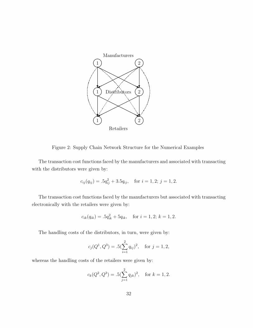
Manufacturers
����1 ����
2
����1 ����
2
����1 ����
2
? ?
HHHHHHHHHHHj
������������
? ?
HHHHHHHHHHHj
������������
Distributors
Retailers
Figure 2: Supply Chain Network Structure for the Numerical Examples
The transaction cost functions faced by the manufacturers and associated with transacting
with the distributors were given by:
cij(qij) = .5q2ij + 3.5qij, for i = 1, 2; j = 1, 2.
The transaction cost functions faced by the manufacturers but associated with transacting
electronically with the retailers were given by:
cik(qik) = .5q2ik + 5qik, for i = 1, 2; k = 1, 2.
The handling costs of the distributors, in turn, were given by:
cj(Q1, Q3) = .5(
2∑
i=1
qij)2, for j = 1, 2,
whereas the handling costs of the retailers were given by:
ck(Q2, Q3) = .5(
2∑
j=1
qjk)2, for k = 1, 2.
32

The bks were set to 100 for both retailers yielding probability distribution functions as in
(59) and the expected demand functions as in (61). The weights associated with the excess
supply and excess demand at the retailers were: λ+k = λ−
k = 1 for k = 1, 2. Hence, we
assigned equal weights for each retailer for excess supply and for excess demand.
Hence, in this example, the manufacturers and the distributors were only concerned
about profit maximization and not with risk minimization. In terms of the model, this
would correspond to (cf. (29)) the weights αi and βj for i = 1, 2; j = 1, 2 equal to zero.
The modified projection method converged and yielded the following equilibrium pattern:
the product shipments between the two manufacturers and the two distributors were: q∗ij =
.3697 for i = 1, 2; j = 1, 2, whereas the product shipments transacted electronically between
the manufacturers and the retailers were: q∗ik = .3487 for i = 1, 2; k = 1, 2, and, finally, the
product shipments between the distributors and the retailers were: q∗jk = .3697 for j = 1, 2;
k = 1, 2. The computed equilibrium prices, in turn, were: ρ∗2j = 15.2301 for j = 1, 2 and
ρ∗3k = 34.5573 for k = 1, 2. The expected demands (see (61)) were: d1(ρ
∗31) = d2(ρ
∗32) =
1.4469.
Example 1b
Example 1b was constructed from Example 1a as follows. We kept the data as in Example
1a but we assumed now that the first manufacturer was a multicriteria decision-maker and
also concerned with risk minimization with his risk function being given by:
r1 = (2∑
k=1
q1k − 2)2
and with the weight α1 = 2. This risk measure can be explained as follows. The first
manufacturer is concerned with physical transactions associated with the retailers and wishes
to increase directly the volume of transactions with the consumers by having the related
shipments lie as close as possible to a target (of 2).
The modified projection method yielded the following new solution: the product ship-
ments between the two manufacturers and the two distributors were: q∗1j = 0.0000, for
j = 1, 2 and q∗2j = .5442 for j = 1, 2. The product shipments transacted electronically
between manufacturers and the retailers were: q∗1k = .7969 for k = 1, 2 and q∗2k = .1327 for
33
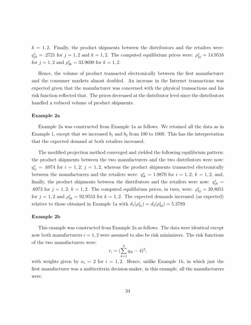
k = 1, 2. Finally, the product shipments between the distributors and the retailers were:
q∗jk = .2721 for j = 1, 2 and k = 1, 2. The computed equilibrium prices were: ρ∗2j = 14.9516
for j = 1, 2 and ρ∗3k = 33.9690 for k = 1, 2.
Hence, the volume of product transacted electronically between the first manufacturer
and the consumer markets almost doubled. An increase in the Internet transactions was
expected given that the manufacturer was concerned with the physical transactions and his
risk function reflected that. The prices decreased at the distributor level since the distributors
handled a reduced volume of product shipments.
Example 2a
Example 2a was constructed from Example 1a as follows. We retained all the data as in
Example 1, except that we increased b1 and b2 from 100 to 1000. This has the interpretation
that the expected demand at both retailers increased.
The modified projection method converged and yielded the following equilibrium pattern:
the product shipments between the two manufacturers and the two distributors were now:
q∗ij = .6974 for i = 1, 2; j = 1, 2, whereas the product shipments transacted electronically
between the manufacturers and the retailers were: q∗ik = 1.9870 for i = 1, 2; k = 1, 2, and,
finally, the product shipments between the distributors and the retailers were now: q∗jk =
.6973 for j = 1, 2; k = 1, 2. The computed equilibrium prices, in turn, were: ρ∗2j = 39.8051
for j = 1, 2 and ρ∗3k = 92.9553 for k = 1, 2. The expected demands increased (as expected)
relative to those obtained in Example 1a with d1(ρ∗31) = d2(ρ
∗32) = 5.3789.
Example 2b
This example was constructed from Example 2a as follows. The data were identical except
now both manufacturers i = 1, 2 were assumed to also be risk minimizers. The risk functions
of the two manufacturers were:
ri = (2∑
k=1
qik − 4)2,
with weights given by αi = 2 for i = 1, 2. Hence, unlike Example 1b, in which just the
first manufacturer was a multicriteria decision-maker, in this example, all the manufacturers
were.
34

The modified projection method converged to the following solution. The product ship-
ments between the two manufacturers and the two distributors were: q∗ij = .6907 for i = 1, 2
and j = 1, 2. The product shipments transacted electronically were: q∗ik = 1.9948 for i = 1, 2
and k = 1, 2, whereas the product shipments between the distributors and the retailers were:
q∗jk = .6906 for j = 1, 2 and k = 1, 2.
The equilibrium prices were: ρ∗2j = 39.7978 for j = 1, 2 and ρ∗
3k = 92.9181 for k = 1, 2.
Note that the volume of products transacted electronically increased from those reported in
Example 2a.
Example 3a
Example 3a was constructed from Example 2a as follows. We retained all the data as in
Example 2a, except that now we decreased the transaction costs associated with transacting
electronically, where now cik(qik) = qik + 1, i = 1, 2; k = 1, 2.
The modified projection method converged and yielded the following equilibrium pattern:
the product shipments between the two manufacturers and the two distributors were now:
q∗ij = .0484 for i = 1, 2; j = 1, 2, whereas the product shipments transacted electronically
between the manufacturers and the retailers were: q∗ik = 2.7418 for i = 1, 2; k = 1, 2, and,
finally, the product shipments between the distributors and the retailers were now: q∗jk =
.0483 for j = 1, 2; k = 1, 2. The computed equilibrium prices, in turn, were: ρ∗2j = 39.1269
for j = 1, 2 and ρ∗3k = 89.4390 for k = 1, 2. Hence, the product shipments between the
manufacturers and the retailers increased and the prices at the retailers decreased (relative
to those obtained in Example 2a).
Example 3b
Example 3b had identical to that of Example 3a except that we added the following data.
In this example the first distributor as a multicriteria decision-maker and concerned with
both profit maximization and risk minimization. His risk function was given by
r1 = (2∑
k=1
q1k − 2)2
with a weight β1 = 1.
35

The modified projection method yielded the following equilibrium solution. The product
shipments between the manufacturers and the distributors were: q∗i1 = .4516 for i = 1, 2 and
q∗i2 = .0128 for i = 1, 2. The product shipments between the manufacturers and the retailers
were: q∗ik = 2.5639 for i = 1, 2 and k = 1, 2. Finally, the product shipments between the
distributors and the retailers were: q∗11 = .4512, q∗12 = .4518 and q∗21 = .0130, q∗22 = .0124.
The equilibrium prices at the distributors’ level were now: ρ∗21 = 40.4076 and ρ∗
22 = 39.0912
whereas those at the retailers’ level were: ρ∗3k = 89.2497 for k = 1, 2.
The above numerical results illustrate the variety of problems that can be solved.
6. Summary and Conclusions
This paper has developed a three-tiered supply chain network equilibrium model consist-
ing of manufacturers, distributors, and retailers with electronic commerce. The model allows
for physical transactions between the different tiers of decision-makers as well as electronic
transactions in the form of B2B commerce between manufacturers and the retailers. In ad-
dition, the demands for the product associated with the retailers are no longer assumed to
be known with certainty but rather, are random. Furthermore, the manufacturers as well
as the distributors are assumed to be multicriteria decision-makers and concerned not only
with profit maximization but also with risk minimization.
The model generalized previous supply chain network equilibrium models to include elec-
tronic commerce, multiple tiers of decision-makers as well as supply side and demand side
risk within the same framework.
Finite-dimensional variational inequality theory was used to formulate the derived equilib-
rium conditions, to study the model qualitatively, and also to obtain convergence results for
the proposed algorithmic scheme. Finally, numerical examples were presented to illustrate
the model and computational procedure.
Future research will include empirical work as well as extensions of the model to global
supply chain networks.
36

Acknowledgments
The research of the first and third authors was supported, in part, by NSF Grant No.:
IIS-0002647 and that of the first and second author also, in part, by a 2002 AT&T Industrial
Ecology Faculty Fellowship. This support is gratefully acknowledged.
The authors thank the two anonymous reviewers for their suggestions and for bringing
to our attention several additional references.
References
V. Agrawal and S. Seshadri, 200. Risk Intermediation in Supply Chains, IIE Transactions
32, 819-831.
M. S. Bazaraa, H. D. Sherali, and C. M. Shetty, 1993. Nonlinear Programming: Theory
and Algorithms, John Wiley & Sons, New York.
V. Chankong and Y. Y. Haimes, 1997. Multiobjective Decision Making: Theory and
Methodology, North-Holland, New York.
M. A. Cohen and S. Mallik, 1997. Global Supply Chains: Research and Applications,
Production and Operations Management 6, 193-210.
J. Dong and A. Nagurney, 2001. Bicriteria Decision Making and Financial Equilibrium: A
Variational Inequality Perspective, Computational Economics 17, 19-42.
J. Dong, D. Zhang, and A. Nagurney, 2002a. A Supply Chain Network Equilibrium Model
with Random Demands, to appear in European Journal of Operational Research.
J. Dong, D. Zhang, and A. Nagurney, 2002b. Supply Chain Networks with Multicriteria
Decision-Makers, in Transportation and Traffic Theory in the 21st Century, M. A.
P. editor, Pergamon Press, Amsterdam, The Netherlands.
J. Dong, D. Zhang, and A. Nagurney, 2003. Supply Chain Supernetworks with Random
Demands, to appear in Urban and Regional Transportation Modeling: Essays in
37

Honor of David E. Boyce, D. -H. Lee, editor, Edward Elgar Publishers, Cheltenham,
England.
J. Dong, D. Zhang, H. Yan, and A. Nagurney, 2003. Multitiered Supply Chain Networks:
Multicriteria Decision-Making Under Uncertainty; see: http://supernet.som.umass.edu
P. Engardio, M. Shari, A. Weintraub, C. Arnst, 2003. Deadly Virus, BusinessWeek Online;
see: http://www.businessweek.com/magazine/content/03 15/b3828002 mx 046.htm
Federal Highway Administration, 2000. E-Commerce Trends in the Market for Freight, Task
3 Freight Trends Scans’, Draft, Multimodal Freight Analysis Framework, Office of Freight
Management and Operations, Washington, DC.
P. C. Fishburn, 1970. Utility Theory for Decision Making, John Wiley & Sons, New
York.
D. Gabay and H. Moulin, 1980. On the Uniqueness and Stability of Nash Equilibria in Non-
cooperative Games, in: Applied Stochastic Control of Econometrics and Manage-
ment Science, A. Bensoussan, P. Kleindorfer, and C. S. Tapiero, editors, North-Holland,
Amsterdam, The Netherlands.
J. Geunes, P. M. Pardalos and H. E. Romeijn, editors, 2002. Supply Chain Manage-
ment: Models, Applications and Research, Kluwer Academic Publishers, Dordrecht,
The Netherlands.
A. Huchzermeier and M. A. Cohen, 1996. Valuing Operational Flexibility Under Exchange
Rate Uncertainty, Operations Research 44, 100-113.
M. E. Johnson, 2001. Learning from Toys: Lessons in Managing Supply Chain Risk from
the Toy Industry, California Management Review 43, 106-124.
R. L. Keeney and H. Raiffa, 1993. Decisions with Multiple Objectives: Preferences
and Value Tradeoffs, Cambridge University Press, Cambridge, England.
D. Kinderlehrer and G. Stampacchia, 1980. An Introduction to Variational Inequali-
38
ties and Their Application, Academic Press, New York.
G. M. Korpelevich, 1977. The Extragradient Method for Finding Saddle Points and Other
Problems, Matekon 13, 35-49.
H. M. Markowitz, 1952. Portfolio Selection, The Journal of Finance 7, 77-91.
H. M. Markowitz, 1959. Portfolio Selection: Efficient Diversification of Investments,
John Wiley & Sons, New York.
A. Nagurney, 1999. Network Economics: A Variational Inequality Approach, second
and revised edition, Kluwer Academic Publishers, Dordrecht, The Netherlands.
A. Nagurney, J. Cruz, and D. Matsypura, 2003. Dynamics of Global Supply Chain Super-
networks, Mathematical and Computer Modelling 37, 963-983.
A. Nagurney and J. Dong, 2002. Supernetworks: Decision-Making for the Informa-
tion Age, Edward Elgar Publishers, Cheltenham, England.
A. Nagurney, J. Dong, and D. Zhang, 2002. A Supply Chain Network Equilibrium Model,
Transportation Research E 38, 281-303.
A. Nagurney, J. Loo, J. Dong, and D. Zhang, 2002. Supply Chain Networks and Electronic
Commerce: A Theoretical Perspective, Netnomics 4, 187-220.
A. Nagurney and S. Siokos, 1997. Financial Networks: Statics and Dynamics, Springer-
Verlag, Heidelberg, Germany.
A. Nagurney and L. Zhao, 1993. Networks and Variational Inequalities in the Formulation
and Computation of Market Disequilibria: The Case of Direct Demand Functions, Trans-
portation Science 27, 4-15.
J. F. Nash, 1950. Equilibrium Points in N-Person Games, in: Proceedings of the National
Academy of Sciences, USA 36, 48-49.
J. F. Nash, 1951. Noncooperative Games, Annals of Mathematics 54, 286-298.
39

National Research Council, 2000. Surviving Supply Chain Integration: Strategies for
Small Manufacturers, Committee on Supply Chain Integration, Board on Manufacturing
and Engineering Design, Commission on Engineering and Technical Systems, Washington,
DC.
P. M. Pardalos and V. K. Tsitsiringos, editors, 2002. Financial Engineering, E-Commerce
and Supply Chain, Kluwer Academic Publishers, Dordrecht, The Netherlands.
Y. Sheffi, 2001. Supply Chain Management under the Threat of International Terrorism,
The International Journal of Logistics Management 12, 1-11.
L. R. Smeltzer and S. P. Siferd, 1998, Proactive Supply Management: The Management of
Risk, International Journal of Purchasing and Materials Management , Winter, 38-45.
F. Southworth, 2000. E-Commerce: Implications for Freight, Oak Ridge National Labora-
tory, Oak Ridge, Tennessee.
J. A. Van Mieghem, 2002. Capacity Portfolio Investment and Hedging: Revoiew and New
Directions, to appear in Manufacturing & Service Operations Management .
P. L. Yu, 1985. Multiple Criteria Decision Making – Concepts, Techniques, and
Extensions, Plenum Press, New York.
D. Zhang and A. Nagurney, 1996. Stability Analysis of an Adjustment Process for Oligopolis-
tic Market Equilibrium Modeled as a Projected Dynamical System, Optimization 36, 263-
285.
G. A. Zsidisin, 2003. Managerial Perceptions of Supply Risk, The Journal of Supply Chain
Management: A Global Review of Purchasing and Supply , Winter, 14-25.
40