Supply chain relational capital and the bullwhip effect

University of Calgary

PRISM: University of Calgary's Digital Repository

Haskayne School of Business Haskayne School of Business Research & Publications

2019-08-15

Supply chain relational capital and the bullwhip

effect: An empirical analysis using financial

disclosures

Zhao, Rong; Mashruwala, Raj; Pandit, Shailendra; Balakrishnan,

Jaydeep

Emerald Group Publishing Limited

Zhao, R., Mashruwala, R., Pandit, S., & Balakrishnan, J. (2018). Supply chain relational capital and

the bullwhip effect: An empirical analysis using financial disclosures. International Journal of

Operations and Production Management. 1-59.

http://hdl.handle.net/1880/110754

journal article

https://creativecommons.org/licenses/by/4.0

Unless otherwise indicated, this material is protected by copyright and has been made available

with authorization from the copyright owner. You may use this material in any way that is

permitted by the Copyright Act or through licensing that has been assigned to the document. For

uses that are not allowable under copyright legislation or licensing, you are required to seek

permission.

Downloaded from PRISM: https://prism.ucalgary.ca

Supply Chain Relational Capital and the Bullwhip Effect: An Empirical Analysis

Using Financial Disclosures

Rong Zhao

Haskayne School of Business


2500 University Dr. NW

Calgary, Alberta, Canada T2N 1N4

[email protected]

Raj Mashruwala





[email protected]

Shailendra (Shail) Pandit

College of Business Administration

University of Illinois at Chicago

Chicago, IL 60607

[email protected]

Jaydeep Balakrishnan





[email protected]

Accepted for publication in the International Journal of Operations and Production

Management

October 2018

mailto:[email protected]



1

Supply Chain Relational Capital and the Bullwhip Effect: An Empirical Analysis

Using Financial Disclosures

ABSTRACT

Purpose: The primary objective of this study is to conduct a large-sample empirical investigation

of how relational capital impacts bullwhip at the supplier.

Design/methodology/approach: The study uses mandatory disclosures in regulatory filings of

US firms to identify a supplier’s major customers and constructs empirical proxies of supply chain

relational capital i.e., length of the relationship between suppliers and customers, and partner

interdependence. Multivariate regression analyses are performed to examine the effects of

relational capital on bullwhip at the supplier.

Findings: The findings show that bullwhip at the supplier is greater when customers are more

dependent on their suppliers, but is reduced when suppliers share longer relationships with their

customers. The results also provide additional insights on several firm characteristics that impact

supplier bullwhip, including shocks in order backlog, selling intensity, and variations in profit

margins. Further, we document that the effect of supply chain relationships on bullwhip tends to

vary across industries and over time.

Originality/value: The study employs a novel dataset that is constructed using firms’ financial

disclosures. This large panel dataset consisting of 13,993 observations over 36 years enables

thorough and robust analyses to characterize supply chain relationships and gain a deeper

understanding of their impact on bullwhip.

Keywords: Bullwhip effect, relational capital, supply chain, regression analysis, financial

statements.

2

1. Introduction

The bullwhip effect (BWE) is considered to be a key phenomenon in supply chain

management. The principal notion of BWE is that demand variability increases as one moves

upstream in a supply chain. This can cause several inefficiencies for the upstream supplier

including poor forecasting, stockouts, high inventory, lower service levels, capacity planning

issues, higher costs, and increased supply chain risk (Metters, 1997; Billington, 2010). The

importance of this problem has prompted extensive research since the early works of Simon (1952)

and Forrester (1958) using theoretical frameworks as well as experimental settings (Kahn, 1987;

Sterman, 1989; Metters, 1997; Lee et al., 1997a, 1997b; and more recently Cao et al., 2017, to

name a few).1 There had not been, however, much large-sample empirical evidence until recent

studies started to use archival data to document the prevalence and the magnitude of the BWE at

the industry and the firm level (e.g., Cachon et al., 2007; Bray and Mendelson, 2012; Shan et al.,

2014; Mackelprang and Malhotra, 2015; and Isaksson and Seifert, 2016). The costs and

inefficiencies linked to BWE underscore the importance of understanding influential factors that

might help mitigate the BWE, an effect that previous studies have shown to exist globally.

In this study, we build on prior research by identifying linkages between supply chain

management research on inter-organizational relationships and research on the BWE. The

‘relational view’ of the firm suggests that close relationships between supply chain partners

engender relational capital, promote mutual trust, and facilitate accurate information flows (Dyer

and Singh, 1998; Cousins et al., 2006). Since the sharing of more accurate information has the

potential to mitigate the BWE (Lee et al., 1997a; Haines et al., 2017), higher relational capital

between supply chain partners should help mitigate the BWE. However, recent research

1 For detailed reviews of the current literature on the bullwhip effect see Miragliotta (2006), Geary et al. (2006),

Towill et al. (2007), Giard and Sali (2013), and Wang and Disney (2016).

3

documents the ‘dark side’ of relational capital and suggests that stronger ties between supply chain

partners may lead to opportunistic or gaming behavior, which has the potential to increase BWE

(Villena et al., 2011; Zhou et al., 2014). The above contrasting views present an interesting

empirical question about the net effect of relational capital on BWE that we investigate in this

study. Accordingly, the principal research question in our study is stated as follows: Does

relational capital between supply chain partners mitigate or exacerbate the bullwhip effect?

The availability of large-scale panel data on customer-supplier relationships offers a unique

opportunity to examine BWE using variation in firm and supply chain characteristics across

different industries and time periods. This can help researchers understand not only the underlying

causes of BWE but also potential mitigating factors that have been theorized to impact BWE.

Consistent with a recent article encouraging the use of archival data (Simpson et al., 2015), we

exploit firms’ financial disclosures of their business relationships to create a dataset that identifies

suppliers and their customers for the period 1978-2013. We measure bullwhip for the supplier

firms in our data using a methodology commonly used in previous studies (e.g., Chen et al., 2000;

Cachon et al., 2007; Shan et al., 2014). Following Krause et al. (2007), we consider three aspects

of relational capital – namely, the length of relationship, customers’ dependence on suppliers, and

suppliers’ dependence on customers – and examine their individual impact on BWE from the

perspective of the supplier.

In our empirical model, we use information obtained from the firms’ financial statements

to measure and control for several supplier characteristics that may potentially impact the BWE.

For example, we include changes in backlogged orders to control for demand shocks that can cause

BWE due to demand signal processing. Variations in suppliers’ gross margins are included to

capture price fluctuations that have been known to cause BWE. We include selling intensity since

we argue that suppliers with high degree of sales-intensive activities are likely to experience higher

4

BWE as salespeople concurrently book larger orders to meet sales targets (Lee et al., 1997a). We

note that large-sample data that is aggregated at the firm level makes it challenging to construct

distinct and unambiguous empirical proxies for specific causes and influential factors for BWE.

Consequently, prior literature does not provide much guidance for measuring such factors using

large-sample data. We use theories embedded in prior literature to guide our choice and

measurement of supplier characteristics while being mindful of the inherent limitations of the data.

Our empirical measures therefore constitute a first attempt and contribute to the literature by

providing a useful starting point for future research that can validate and improve on these

measures.

We find that longer relationships lead to lower BWE at the supplier. While suppliers’

dependence on customers has no significant effect on bullwhip, customers’ dependence on

suppliers results in greater bullwhip at the supplier. The latter result is suggestive of an increase in

gaming behavior such as duplicate or “phantom” ordering when customers are dependent on a

specific supplier (Sterman and Dogan, 2015; Armony and Plambeck, 2005; Mitchell, 1924). These

results are not only new to the literature, but also provide direction to practitioners in terms of

being able to manage their supply chains more effectively.

Our multivariate regression analysis of the drivers of BWE also shows that higher selling

intensity, higher variations in gross margin, and greater shocks to order backlogs are associated

with greater bullwhip at the supplier. Similar to Shan et al. (2014) we use additional controls

including serial correlation in demand, days in inventory, supplier size, supplier profit margin,

days payable outstanding, and seasonality. We confirm Shan et al.’s (2014) findings for Chinese

firms in our sample of US firms. For example, we find that higher serial correlation in demand and

longer inventory days are associated with larger BWE in US firms.

5

In the next section we present a brief overview of the related literature and our research

hypotheses. This is followed by a description of our data, sample, and our empirical results. In the

subsequent section we discuss the managerial implications of our results. Finally, we present our

concluding remarks.

2. Literature review

2.1. Evidence of the BWE

The BWE has been extensively studied in a variety of theoretical and experimental settings.

The formal evidence on BWE has been corroborated by several instances of real-world evidence.

For instance, Procter and Gamble (P&G) observed the BWE phenomenon with its suppliers and

wholesalers (Schisgall, 1981). Lee et al. (1997a) document the experience of Hewlett-Packard

(HP) which found that orders received from a major printer distributor had much bigger swings

than fluctuations in the sales of the distributor. Dooley et al. (2010) found that during 2007-2009,

demand variation due to the economic recession was larger for manufacturers than for retailers,

which is indicative of the BWE. Evidence of BWE has been found in other countries as well. For

example, Bu et al. (2011) report the existence of BWE in the Chinese manufacturing sector,

providing evidence of significant cross-sectional differences in the extent of BWE across

industries. Amplification of demand variance has been observed in several studies focusing on

specific firms or product categories, including apparel (Stalk and Hout, 1990), groceries

(Hammond, 1994; Panda and Mohanty, 2012), automotive (Taylor, 1999), perishable foods

(Fransoo and Wouters, 2000), mechanical parts (McCullen and Towill, 2001b), toys (El-Beheiry

et al., 2004), printers (Disney et al., 2013), retail (Lai, 2005), and spare parts (Pastore et al., 2017).

In one of the first large-sample investigations of BWE, Cachon et al. (2007) document

BWE using industry-level data from the US Census Bureau. They compare the amplification of

production variance relative to demand variance for retail, wholesale and manufacturing industry

6

groups. Cachon et al. (2007) find some evidence that BWE exists for wholesale industries but not

for manufacturing and retail industries. As they note, “[H]owever, it is not possible to conclude

from industry-level volatility whether amplification occurs at the firm, division, category or

product-level (p. 477)”. Firms within an industry could belong to different tiers of the supply chain.

For instance, within the pharmaceuticals industry firms could exist at different tiers such as large,

diversified manufacturers and marketers (e.g., Merck), which are served by upstream

biotechnology firms developing new drugs (e.g., Micromet), which in turn buy technical knowhow

or materials from suppliers even further upstream (e.g., Curis). When information for firms

belonging to different supply chain tiers is aggregated at the industry level, information regarding

the firm’s placement in the supply chain is lost. Hence, the analysis using aggregate industry-level

data could mask the underlying supply chain relationships. Also, industry-level analysis leads to a

smaller set of data points, which reduces the statistical power of empirical tests.

More recently, Bray and Mendelson (2012) investigate the BWE at the firm rather than the

industry level by developing a firm-level measure of amplification of demand signals. Using a

sample of US companies, they find significant demand amplification for 65 percent of the firms in

their sample, while for the remaining firms there is no BWE. This shows that there are significant

cross-sectional differences in the BWE across the sample. In another study focusing on Chinese

firms, Shan et al. (2014) document similar results – two-thirds of the firms in their sample exhibit

demand amplification. Isaksson and Seifert (2016) replicate these findings in US firms, providing

strong evidence of the magnitude and prevalence of BWE across industries. However, none of the

above studies exploit characteristics of specific supplier-customer relationships to examine their

impact on BWE. Our study helps fill this gap in the literature.

7

2.2. Relational Capital and BWE

The BWE literature has also focused on identifying causes and factors that influence BWE

with the intent of providing insights that may be useful to managers in reducing the impact of

BWE. Lee et al. (1997a; 1997b) adopt the view that BWE results from managers acting rationally

in responding to demand signals. They identify four distinct causes of the BWE, namely, demand

signal processing, order batching, supplier rationing, and price variations. These causes have since

been accepted as the standard explanation for the existence of BWE in empirical settings (e.g.,

Miragliotta, 2006). In addition to the direct causes of the BWE, Lee et al. (1997a) speculate about

the counter measures that would help reduce the BWE. For example, greater demand information

sharing between supplier and customer is likely to mitigate the BWE. Lee et al. (1997a, 1997b)

provide an example of the grocery industry where electronic data interchange (EDI) systems

facilitate greater information sharing between the retailer and the supplier, and provide the supplier

with greater visibility of the end consumer demand, thus reducing BWE. Other studies add support

to the view that information sharing and cooperation between the supplier and customer reduce

BWE (e.g., Gavirneni et al., 1999; Zhao and Xie, 2002).

Much of the supply chain literature over the past two decades has examined customer-

supplier relationships through the lens of relational theory. The theory describes how information

sharing is impacted by close relationships between supply chain partners. Relational capital is

developed through a history of interactions between partner firms, enabling the partners to earn

various benefits or ‘relational rents’ that may not otherwise be available to them (Nahapiet and

Ghoshal, 1998; Krause et al., 2007; Yim and Leem, 2013). Closer relations between suppliers and

customers lead to improved communications (Hoetker, 2005), development of relationship-

specific information-sharing routines (Dyer and Singh, 1998), and greater trust between partners

(Helper, 1991; Sako and Helper, 1998). Thus, as relational capital grows, greater trust and better

8

communication between partners will help facilitate the flow of potentially useful and important

information quickly and accurately through the network (Cousins et al., 2006). With greater trust,

such information flows would be transmitted upstream in a more timely fashion, potentially

reducing the propagation of BWE (Lee et al. 1997a). Thus, in the context of BWE, relational

capital, as represented by the length of the supplier-customer relationship and the interdependency

of the customer and supplier (Krause et al., 2007), can be expected to be negatively related to the

BWE.

However, recent research also documents the potential negative consequences of relational

capital, which can include opportunistic behavior (Granovetter, 1985) and restricted information

flows (Villena et al., 2011). When the customer has a high level of trust in the supplier, the

customer may reduce its monitoring of the supplier (Villena et al., 2011). Responding to lower

customer monitoring, the supplier may reduce sharing of critical information with the customer

(Zhou et al., 2014). Additionally, if a customer becomes reliant on a limited number of suppliers,

then in times of short supply the customer might resort to placing phantom orders to ensure supply.

When the customer gets adequate delivery, it cancels outstanding orders, causing BWE to

propagate through the supply chain. This type of phantom or duplicate ordering has been well-

documented in the literature (Sterman and Dogan 2015; Lee et al. 1997b; Armony and Plambeck

2005; Mitchell 1924), and has been seen in many industries such as electronic components,

consumer electronics, and personal computers (Lee et al., 1997a); and semiconductors (Terwiesch

et al., 2005). Hence, such opportunistic behaviors combined with restricted information flows

could lead to an increase, rather than a reduction, in BWE with higher relational capital. Therefore,

given that relational capital can have a mixed impact on BWE, the net effect of relational capital

on BWE remains an empirical question, which forms the basis of our research hypotheses.

9

3. Hypothesis development

In this section we develop specific hypotheses regarding the impact of three distinct aspects of

relational capital – namely the length of the relationship between suppliers and customers,

customers’ dependence on suppliers, and suppliers’ dependence on customers (Krause et al., 2007)

– on BWE.

3.1. Length of relationship between customers and suppliers

In the traditional model of supplier-customer relationships, customers frequently changed

suppliers in search of lower prices (Lamming, 1993). The lack of sustained relationships likely led

to poor information flows between customers and suppliers (Langfield-Smith and Greenwood,

1998). However, starting in the mid-1980s, there was a growing recognition in the US and other

developed economies of the importance of building collaborative long-term relationships with

suppliers. Automotive companies, largely emulating their Japanese counterparts, adopted aspects

of ‘just-in-time’ (JIT) or ‘lean’ supply chain practices that preferred longer-term contracts.

Describing this move towards Lean Management, Schonberger (1982, p157) states, “the Japanese

tend to buy from the same few suppliers year after year, so that the suppliers develop a competency

that is particularly attuned to the delivery and quality needs of the buying firm. Confidence in the

supplier reduces buffer inventories carried in the buying plans to quantities that are used up in only

a few hours.”

The practice of lean management led to greater information sharing and stronger

relationships between customers and suppliers (Langfield-Smith and Greenwood, 1998), which in

turn, helped suppliers improve their performance.2 In a study of both Japanese and U.S. automotive

manufacturers and suppliers, Kotabe et al. (2003) find that both knowledge transfer and supplier

2 See Bhamu and Sangwan, (2014) for a review of studies on lean manufacturing and how customer-supplier

relationship strength promotes lean implementation success.

10

performance improve with longer relationships. Examining first-tier US suppliers to both US-

based Japanese as well as US automakers, Liker and Yen-Chun (2000) show that closer and longer-

term relationships that existed with Japanese automakers led to more stable production. MacDuffie

and Helper (1997) document the case of Honda USA and its supplier Progressive Industries.

Progressive had experienced cyclical demand traditionally, but after building up its relationship

with Honda over time it was able to move to a more stable production schedule. McCullen and

Towill (2001a) discuss the case of a British manufactured products supplier (primarily to USA and

Japan) that implemented agile systems (including lean, and closer relationships with customers)

and experienced significant attenuation in BWE. Similarly, Pozzi et al. (2018) consider the benefits

of lean management in the case of a beer game supply chain and find that lean thinking helps in

reducing BWE.

Following this trend towards longer customer-supplier relationships engendered by lean

management, more recent studies in the supply chain management literature use the relational view

to examine the costs and benefits of collaborative relationships between suppliers and their

customers. Long-term relationships result in investment in relationship specific assets (De Toni

and Nassembini, 1999; Prajogo and Olhager, 2012), more information sharing, logistics

integration, and better performance (Prajogo and Olhager, 2012). The literature on relational

capital suggests that repeated interactions between supply chain partners influence their respective

behaviors. These interactions are a prerequisite for the creation of trust (Li et al., 2014). The

increased trust tends to improve communication and information sharing (Hoetker, 2005). For

instance, Toyota encourages frequent interactions between its employees and those of its suppliers

to encourage information transfer (Adler et al., 2009; Liker and Choi, 2004). Through these

interactions the customer and the supplier are able to develop relational ties, building trust in one

another, that are instrumental in promoting two-way information flows and improving operational

11

efficiency such as lead time (Cousins and Menguc, 2006). The supply chain partners could share

information about market demand, production planning, and inventory (Li and Lin, 2006).

Relational capital encourages not just higher quantity, but also the quality, of the shared

information such as accuracy and timeliness (Li et al., 2014). Further, this increased

communication results in enhanced relational assets (Kotabe et. al., 2003).

The bullwhip effect is created when an upstream supplier processes demand input from

their immediate downstream customer in producing their own forecasts. However, as Lee et al.

(1997a) suggest, if the customer shares accurate data on end-demand with the supplier on a

frequent basis, this is likely to reduce the impact of BWE at the supplier. For instance, supply chain

partners can use electronic data interchange (EDI) or other information integration methods (as

was the case with the British supplier in McCullen and Towill, 2001a) to share raw demand data

on a timely basis. The reduction of operational lead times is also likely to reduce BWE at the

supplier (Lee et al., 1997b). Hence, we posit that the improved information sharing (both quality

and quantity), and the reduction of lead times due to the longer relationships between suppliers

and customers, will serve to reduce the impact of BWE at the supplier.

Nonetheless, researchers have cautioned against the potential risks and negative

consequences associated with longer relationships between suppliers and customers. Longer

relationships could lead to relational inertia (Villena et al., 2011) by locking both parties into

relationships with restricted information flows and increasing the risk of opportunistic exploitation

(Yan and Kull, 2015). Agency theory and transaction cost theory indicate that monitoring acts as

a safeguard against opportunism and is useful in reducing information asymmetry (Bergen et al.,

1992; Wathne and Heide, 2000). However, high levels of trust in long-term relationships can

reduce the monitoring efforts of partner firms. This may potentially slow the sharing of critical

information amongst supply chain partners, and also lead to more opportunistic behavior (Zhou et

12

al., 2014). These negative consequences may counteract the positive effects of longer relationships

on supplier BWE. We examine this issue in our first set of two-sided research hypotheses which

we state as follows:

Hypothesis (H1a): The longer the relationship between the supplier and its customers,

the lesser will be the supplier bullwhip.

Hypothesis (H1b): The longer the relationship between the supplier and its customers,

the greater will be the supplier bullwhip.

3.2. Dependence on Suppliers

Customers’ dependence on suppliers can influence the BWE in two distinct ways. The

relational view of the firm (Dyer, 1996; Madhok and Tallman, 1998) suggests that the customer

accrues tangible benefits from investing in and sharing knowledge with suppliers via reduced

costs, greater quality and flexibility (Yao and Zhu, 2012). If a customer is dependent on a given

supplier for a bulk of its purchases, then the customer will be more willing to invest in relationship-

specific assets and supplier development through information sharing (Krause et al., 1998). For

example, collaborative planning, forecasting, and replenishment (CPFR) is a technique for

coordinating the supply chain (Panahifar et al., 2015). These benefits to the customer are likely to

be the greater, the more dependent a customer is on a given supplier. Since these relationship-

specific investments by the customer that promote greater information sharing require an outlay

of fixed costs, the customer is more likely to share information with only its major suppliers. This

provides suppliers with greater visibility of end-demand conditions, leading to a reduction in

bullwhip at the supplier.

However, when customers are dependent on a limited set of suppliers, this leads to small

number bargaining problem (Clemons et al., 1993). Such negative effects of a dependency

relationship are seen while implementing JIT. Frazier et al. (1988, p.60) noted that the “coercive

use of power in interfirm relationships seriously weakens their collaborative nature.” When there

13

are only few potential suppliers for a product, this also increases the potential for gaming behavior

such as phantom ordering (Armony and Plambeck, 2005; Zarley and Damore, 1996) and rationing

(Lee et al., 1997a,b) which can increase BWE at the supplier. When a customer is dependent on a

supplier, and the supplier is unable to fill all orders, customers may respond by ordering more than

their needs (Sterman and Dogan, 2015). This phenomenon is well-documented in the literature and

is often referred to as phantom ordering (Mitchell, 1924). After a lag, once the customers get all

the products they need, customers will cancel their phantom orders. Such phantom ordering

followed by cancellation of duplicate orders distorts the demand pattern of the supplier leading to

bullwhip. Anecdotal evidence of this phenomenon is found in de Kok et al. (2005) where they

describe the BWE reduction efforts undertaken by Philips Semiconductors, one of the largest

suppliers of semiconductors in the world. Presumably, the customers of Phillips depended heavily

on it as a supplier. de Kok et al. (2005) indicate that customers had been shortage gaming Philips

before the latter undertook deliberate efforts to reduce such behavior by its customers.

Thus, there are two countervailing forces at work when customers are dependent on

suppliers. While information sharing and cooperation can serve to reduce bullwhip at the supplier,

the increased potential for gaming behavior can lead to greater bullwhip. The net effect of these

two forces remains an empirical question which we address in our next hypothesis. To

accommodate a two-sided hypothesis, we present it as follows:

Hypothesis (H2a): The dependence of customers on a given supplier has a negative

impact on supplier bullwhip.

Hypothesis (H2b): The dependence of customers on a given supplier has a positive

impact on supplier bullwhip.

3.3. Dependence on Customers

Suppliers’ dependence on customers (i.e., customer concentration) can also affect bullwhip

at the supplier. We illustrate this impact using a simple example. Let us consider two supplier-

14

customer pairs S1-C1 (i.e., S1 supplies to C1) and S2-C2 (S2 supplies to C2). Suppose, firm S1

supplies to only one customer while firm S2 supplies to multiple customers, with customer C2

constituting only a small percentage of S2’s customer base. Both customers will transmit bullwhip

upwards, reflected in increased production variance for their respective suppliers. However, the

effect of C2’s bullwhip on S2’s total production will be relatively muted since demand from

customer C2 only accounts for a small percentage of S2’s total production. To the extent individual

bullwhips transmitted by firm S2’s multiple customers are not perfectly positively correlated, S2

should experience a lower degree of bullwhip compared with S1 who is fully exposed to the

bullwhip from a single customer C1. In sum, when suppliers are more dependent for their sales on

a few customers, this creates greater uncertainty for the supplier. In a study of over 450 grocery

suppliers, Panda and Mohanty (2012) found that a number of suppliers depended on a limited

number of supermarket chains for a significant portion of their revenues, which led to an increase

in BWE at the supplier.

The above argument is not without tension. If a supplier is highly dependent on a customer

then they are more likely to cooperate closely with customers, as discussed in the relational view

above. For example, Carr et al. (2008) find in a multi-industry survey that such dependence tends

to increase suppliers’ participation in training and involvement during product development. Such

collaborative behavior allows supply chain participants to jointly gain a clear understanding of

future demand and to coordinate their activities accordingly (Wu et al., 2014). Suppliers are also

more likely to make investments in information technology (e.g., EDI) that promote information

sharing (Disney and Towill, 2003) and reduce the impact of bullwhip (Zhang and Chen, 2013).

Asanuma (1989) provides an example from the Japanese auto industry where parts manufacturers

depend on large customers such as Toyota. Despite the size differences, information regarding

15

demand is shared by the customer with the supplier, due to close relationships that exist in the

Japanese auto industry.

Hence, similar to the case of customers’ dependence on their suppliers, the net effect of

customer concentration for reducing supplier bullwhip is an empirical issue due to the presence of

some factors that alleviate the BWE but other factors that exacerbate it. Consistent with hypothesis

H2, we present our next set of two-sided hypotheses as follows:

Hypothesis (H3a): The dependence of a supplier on its customers has a negative impact on

supplier bullwhip.

Hypothesis (H3b): The dependence of a supplier on its customers has a positive impact

on supplier bullwhip.

4. Sample selection and empirical results

4.1. Sample selection

We identify supplier-customer relationships at the supplier-fiscal year level during 1978-

2013 using the Segment Customer File in Standard & Poor’s COMPUSTAT database. Under

Statement of Financial Accounting Standards (SFAS) No. 14 and No. 131, a supplier is required

to disclose the identity and the amount of revenue from a single external customer when revenue

from this customer amounts to 10 percent or more of the supplier’s total revenue. Suppliers also

often disclose information about customers that account for less than 10 percent of suppliers’ total

revenues if they consider them to be major customers (Patatoukas, 2012). The Segment Customer

File contains the names of major customers along with the amount of revenue from each major

customer.

We match each customer’s name to a firm listed on the COMPUSTAT Industrial files.

Following Bray and Mendelson (2012), we focus on retail, wholesale, manufacturing and resource

extracting sectors (SIC 5200-5999, 5000-5199, 2000-3999, and 1000-1400). Our preliminary

sample includes 30,279 supplier-customer pairs at the fiscal year level comprising 3,934 (1,594)

16

unique suppliers (customers). Table 1 presents the data requirements we impose on this

preliminary sample to arrive at the regression sample. We eliminate 5,377 observations where we

do not have sufficient data to measure the BWE for suppliers and 1,610 observations where we do

not have sufficient data on supplier-customer relationship. These steps result in 23,292 supplier-

customer pairs which we aggregate (across multiple customers) to arrive at a sample of 16,746

supplier-year observations. Requiring sufficient data to construct other influential factors and

control variables further eliminates 2,753 observations. Our final sample includes 13,993 supplier-

year observations for 2,786 unique suppliers.

------------------------- Insert Table 1 Approximately Here ------------------------

4.2. Measurement of bullwhip effect

Cachon et al. (2007) measure BWE at the industry level using U.S. Census Bureau data.

They interpret “production” as the inflow of material from upstream suppliers to an industry (or

the demand an industry imposes on its upstream suppliers), and margin-adjusted aggregate

industry sales as the “demand” imposed on an industry by its downstream customers. Cachon et

al. (2007) construct amplification ratio as the variance of monthly production divided by the

variance of monthly margin-adjusted sales to customers. Measuring BWE at the firm level using

quarterly financial statement data from COMPUSTAT, Bray and Mendelson (2012) and Shan et

al. (2014) define BWE as the variation of production relative to the variation of demand. Similar

to prior studies, we measure the bullwhip for a given supplier in a given year as follows:

𝐵𝑊𝐸 =𝜎(𝑃𝑅𝑂𝐷𝑈𝐶𝑇𝐼𝑂𝑁)

𝜎(𝐷𝐸𝑀𝐴𝑁𝐷) (1)

𝜎(𝑃𝑅𝑂𝐷𝑈𝐶𝑇𝐼𝑂𝑁) is the standard deviation of quarterly PRODUCTION in a fiscal year and

𝜎(𝐷𝐸𝑀𝐴𝑁𝐷) is the standard deviation of quarterly DEMAND in a fiscal year. Following Bray

and Mendelson (2012) and Shan et al. (2014), we use cost of goods sold (COGS) as the proxy for

17

customer orders or demand, and COGS plus changes in inventory (INVT) as the proxy for

production. Similar to Cachon et al. (2007) and Shan et al. (2014), we log and first difference

production and demand. That is, for every firm-quarter, production or demand is transformed into

{ln(Xt) – ln(Xt-1)}, which we label as PRODUCTION and DEMAND in equation (1). The BWE

measured in (1) indicates the variation of production upstream as a ratio of the downstream demand

variation. Hence, values greater than one indicate amplification of demand information.

The use of firm level, rather than product-level, demand and production data poses some

challenges. Ideally, researchers would like to link the variance in demand for an individual product

at a downstream customer with the variance of production of the same product by an upstream

supplier. However, product-level data is not readily available, leading to the use of industry-level

or firm-level data in prior research (see, e.g., Cachon et al., 2007; Bray and Mendelsohn, 2012;

and Mackelprang and Malhotra, 2015). At the customer firm level, demand and production data

aggregates different product lines supplied by a number of suppliers which are likely to exhibit

varying degrees of variance amplification. Empirically, however, such comingling of multiple

demand and production streams is expected to increase the noise (alternatively, diminish the signal

to noise ratio), thus biasing against finding results.

4.3 Measuring supply chain relational capital

4.3.1 Length of relationship between customers and suppliers

The mandatory disclosures required in a supplier firm’s annual regulatory filings allow us

to measure the number of years that the supply chain relationship existed using the following

equation:

𝐶𝑆_𝐿𝐸𝑁𝐺𝑇𝐻𝑖𝑡 =∑ (𝑤𝑖𝑗𝑡×𝑌𝐸𝐴𝑅𝑖𝑗𝑡)

𝐽𝑗=1

∑ 𝑤𝑖𝑗𝑡𝐽𝑗=1

(2)

𝑤𝑖𝑗𝑡 = 𝐶𝑆𝐴𝐿𝐸𝑖𝑗𝑡

𝑆𝑆𝐴𝐿𝐸𝑖𝑡 (3)

18

CS_LENGTH is the length of the relationship between the supplier i and its customers in year t,

measured as the number of years that the supplier-customer relationship has existed, scaled by the

number of years since the customer first appeared in the sample (denoted YEAR).3,4 For any

supplier that reports multiple major customers in a given year, we use the weighted-average length

of the relationship where the weight (wijt) is the relative importance of each major customer to the

supplier based on sales to customer j (CSALEijt) divided by the supplier i’s total sales in year t

(SSALEit).

4.3.2. Customers’ dependence on suppliers

CSALE_CCOGS, captures the degree of customers’ exposure to the supplier (Pandit et al.,

2011) and it is calculated as follows:

𝐶𝑆𝐴𝐿𝐸_𝐶𝐶𝑂𝐺𝑆𝑖𝑡 =∑ (𝑤𝑖𝑗𝑡×

𝐶𝑆𝐴𝐿𝐸𝑖𝑗𝑡

𝐶𝐶𝑂𝐺𝑆𝑗𝑡)

𝐽𝑗=1

∑ 𝑤𝑖𝑗𝑡𝐽𝑗=1

(4)

CSALEijt is defined as before and CCOGSjt is cost of goods sold reported by customer j in year t.5

Similar to how we construct CS_LENGTH, for any supplier that reports multiple major customers

in a given year, we average across the customer using the relative importance of each major

customer to the supplier as the weight.

3 Consistent with the approach in Hertzel et al. (2008), we assume that the supplier-customer relationship continues

if the gap between two identified relationship years is less than five. 4 For some observations in our sample (less than 8% of the data) the first year that the relationship between a supplier

and customer is identified is the same as the first year that the customer exists in the database. For these observations,

YEARijt is equal to one for the supplier-customer pair throughout the sample period, thus implying that the customer

and supplier maintain a relationship for the entire period of the customer’s existence. As a robustness check, we

eliminate observations where YEARijt remains one and rerun our regressions. Our results (untabulated) remain robust. 5 Since customers and suppliers are linked based on fiscal year our measurement could be affected by a mismatch

resulting from customers and suppliers reporting in different months of the fiscal year. However, in our sample of

23,292 dyads, the median difference in the fiscal year end of suppliers and their customers is 31 days, which suggests

that for the majority of suppliers and customers their fiscal year ends are not far apart even if they do not report on the

same month. As a robustness check, we construct an alternative CSALE_CCOGS as follows. First, we match the

supplier’s fiscal year end with the customer’s closest fiscal quarter end (quarter t). We then replace the customer’s

annual cost of goods sold with the sum of past 4 quarters of cost of goods sold (quarters t, t-1, t-2 and t-3) and

recalculate CSALE_CCOGS. The correlation between this alternative measure and our original measure is 0.986. Our

results are robust to using this alternative measure (untabulated).

19

4.3.3. Suppliers’ dependence on customers

We measure supplier’s dependence on the customer using a variable developed by

Patatoukas (2012) to measure customer-base concentration (CCONC) which is calculated as

follows:

𝐶𝐶𝑂𝑁𝐶𝑖𝑡 = ∑ (𝐶𝑆𝐴𝐿𝐸𝑖𝑗𝑡

𝑆𝑆𝐴𝐿𝐸𝑖𝑡)

2𝐽𝑗=1 (5)

where CSALEijt is sales from supplier i to customer j in year t and SSALEit is total sales reported

by supplier i in year t. CCONC is determined by the number of major customers and the relative

importance of each major customer to the supplier. Similar in spirit to the Herfindahl-Hirschman

index, higher values of CCONC indicate a more concentrated customer base, and thus greater

dependence of the supplier on its customers.

4.4. Controlling for Supplier Characteristics

In our empirical models, we include controls for other supplier characteristics that could

influence BWE. We develop measures for these characteristics based on financial disclosures.

While some of these are new to the literature, we also include other characteristics that have been

used as control variables in prior studies. We describe these control variables below.

Order Backlog

One of the known and documented causes of BWE is demand signal processing by the

supplier (Lee et al., 1998b). If a supplier experiences a demand shock in one period, it will interpret

this as a signal of high future demand, and order more than the observed sales leading to BWE.

We use order backlogs disclosed by the supplier to control for such demand shocks. Order backlog

reflects customer orders that have been received by the supplier but have not been completed as of

the reporting date. Firms are required to disclose the dollar amount of order backlog based on SEC

20

regulations on an annual basis (Rajgopal et al., 2003)6. The level of order backlog for a firm in a

given year is likely to be driven by industry factors or firm characteristics such as the firm’s

business model (Chang et al., 2018). However, any demand shock will result in a change in the

order backlog (from the prior period) assuming that the operating capacity of the supplier remains

fixed in the short run. Hence, we capture order fluctuations using the changes in order backlog

(BACKLOG). Since we are interested in controlling for the variation in order backlog, we do not

distinguish between positive shocks and negative shocks, and measure BACKLOG using the

absolute difference between supplier’s current year backlog and prior year backlog, scaled by total

assets.

Variation in Gross Margin

We use variation in gross margins (CV_GM) to control for price variations that can cause

bullwhip. CV_GM is the coefficient of variation in a supplier’s deseasonalized gross margin (gross

profit divided by net sales) measured using four quarters of data in any given year. A lowering of

the selling price is likely to reduce the supplier’s gross margins, while an increase will result in an

increase in the gross margins. To the extent such discounts or price increases are temporary, they

will introduce a greater degree of variation in the supplier’s gross margin compared with suppliers

who offer steady prices. The variation in gross margin can also be driven by changes in the costs

of goods sold (COGS). However, changes in COGS alone are not likely to contribute to the BWE.

It is the variation in customer demand driven by price variation that is a primary cause of the BWE.

If margin variations are driven not by price variation but by changes in COGS, we would not

expect to find a relation between the variation in gross margin and the BWE.

Selling Intensity

6 Since order backlog is reported only in annual financial statements, this measure may not capture all demand shocks

that occur during the year.

21

Incentive contracts of salespersons and executives typically involve a nonlinear

relationship between compensation and sales and/or profits with bonuses received when the

employee reaches a minimum threshold at the end of the fiscal period (Oyer, 1998). This creates

incentives to manipulate the timing of purchases by customers to reach the required thresholds

before the fiscal period ends (Oyer, 1998). Consistent with this observation, Lee et al. (1997b)

state that providing such sales incentives pushes salespeople to close deals towards the end of a

period to reach their sales targets. This results in a positive correlation of sales orders from different

salespeople. The variance of orders received by the supplier from multiple customers is highest

when the orders are correlated, thus giving rise to BWE (Lee et al., 1997b). Prior literature finds

that firms that have high selling intensity are more likely to offer incentive plans to salespersons

(John and Weitz, 1989). Thus, we include a control for selling intensity in our empirical models to

capture the extent of sales incentives provided to salespersons. 7 We define selling intensity

(SGA_INTENSITY) as the amount of annual selling and general administrative expenses (SG&A)

divided by annual net sales.

Other Control Variables

In addition to these three variables that capture the operational characteristics of suppliers,

we also include additional controls that are included in Shan et al. (2014): serial correlation in

demand, inventory lead times, seasonality, supplier size, supplier profit margin, and account

payable days. As discussed in Lee et al. (1997a,b), demand signal processing is a primary cause

of the BWE. A firm creates an order to its supplier by forecasting future demand (often using

demand smoothing techniques) and incorporating safety stock considerations. This distorts the

7 Selling intensity may be a noisy proxy for incentives offered to salespersons that might cause BWE, since it is also

related to the efficiency/slack of a firm’s marketing resources. While we use this measure as a control in our main

analysis, we also check the robustness of our results in a model that excludes this control variable. In untabulated

results, we find that our inferences are not altered by the exclusion of this control variable from our analysis.

22

original market demand information and amplifies the variance of the firm’s order to its supplier.

The variance amplification increases upstream as the supplier aggregates orders from customers

and adds its own safety stock. In the Lee et al. (1997a,b) framework, this amplification is further

exacerbated if: (1) demand is serially correlated, because then temporary surges in demand are

interpreted by suppliers as signals of high future demand,8 and (2) lead times are longer, because

of the necessity for additional safety stock inventory. Consistent with the above logic, Shan et al.

(2014) report a significantly positive relation between serial correlation in demand and the BWE.

Similar results are found in Cachon et al. (2007). Hence, we include serial correlation in demand

shocks (AR1RHO) in our empirical investigation. AR1RHO is the autoregressive coefficient

estimated with deseasonalized DEMAND series using eight quarters of data.

The other empirical proxy related to demand signal processing is inventory lead time. Prior

studies such as Shan et al. (2014) argue that high inventory days can indicate a firm’s inability to

forecast demand, which leads to higher BWE. Hence, we include inventory days (DAYSINVT) in

our empirical investigation to confirm this well-established result. DAYSINVT measures how many

days a supplier holds its inventory before selling. We expect to find that the BWE is greater when

there is greater serial correlation in demand shocks, and when inventory days are higher.

Shan et al. (2014) also find that the BWE is negatively associated with the seasonality of

demand, thus we control for SEASONALITY which is calculated as the difference between the

variance of DEMAND and the variance of deseasonalized DEMAND, divided by the variance of

DEMAND. The remaining control variables are SIZE which is the supplier’s total assets, GM

8 Alternatively, high serial correlation could make it easier to anticipate future demand, resulting in more accurate

demand forecasts. In the extreme case of perfect correlation, the firm can make a naïve yet accurate forecast.

23

which is the supplier’s gross margin, and DAYSAP which is the number of days a supplier takes to

pay its accounts payable.9

4.5 Regression specifications

To investigate the influential factors for the BWE, we estimate the following ordinary least

squares (OLS) regression with industry sector fixed effects and cluster the standard errors on two

dimensions (firm and year) following Petersen (2009):

𝐵𝑊𝐸𝑖𝑡 = 𝛽0 + 𝛽1𝑙𝑛(𝐶𝑆_𝐿𝐸𝑁𝐺𝑇𝐻𝑖𝑡)+𝛽2𝑙𝑛(𝐶𝐶𝑂𝑁𝐶)𝑖𝑡+𝛽3𝑙𝑛(𝐶𝑆𝐴𝐿𝐸_𝐶𝐶𝑂𝐺𝑆)𝑖𝑡

+ ∑ 𝛾𝑘𝐶𝑜𝑛𝑡𝑟𝑜𝑙𝑘𝐾𝑘=1 + ∑ 𝛼𝑚𝐼𝑛𝑑𝑢𝑠𝑡𝑟𝑦𝑚

𝑀𝑚=1 + 𝑒𝑖,𝑡 (6)

Subscripts i and t indicate supplier firm i and fiscal year t, respectively. BWE is the bullwhip effect

experienced by the supplier as previously defined. ln(CS_LENGTH), ln(CCONC) and

ln(CSALE_CCOGS) are empirical measures for the length of the supplier-customer relationship,

dependence on customers, and dependence on suppliers, respectively. We control for other

influential factors that may affect BWE including ln(SGA_INTENSITY), ln(BACKLOG), and

ln(CV_GM). We use natural log transformation of these influential factors to mitigate the skewness

of these variables.10 We also control for variables that Shan et al. (2014) have shown to be

associated with the BWE - AR1RHO, ln(DAYSINVT), ln(SIZE), ln(GM), ln(DAYSAP) and

SEASONALITY. Following Shan et al. (2014), all control variables except AR1RHO and

SEASONALITY are also log-transformed to mitigate the skewness. Finally, we include indicator

variables for industry sectors to account for unobservable industry heterogeneity and to control for

shocks common to all firms in an industry that can produce a cross-correlation of residuals across

firms in the same industry.

9 Shan et al. (2014) measure firm size using sales in their tabulated results and disclose in an endnote that their results

are robust to using fixed assets or the number of employees as alternative proxies. Since sales are highly correlated

with cost of goods sold that is used in the construction of the BWE, we use assets to proxy for size. 10 We add one to BACKLOG before log-transformation to accommodate observations with zero BACKLOG.

24

Research designs relying on panel data sets, i.e., those containing observations on multiple

firms over multiple years, can be subject to two forms of correlation across observations. The

residuals of a given firm may be correlated across years for that firm (time-series dependence), or

the residuals of different firms may be correlated in a given year (cross-sectional dependence). In

the case of correlated residuals, the true variability of the coefficient estimates is likely to be

misestimated by OLS standard errors. An option considered in the literature is to use firm and year

fixed effects to correct for this issue. However, our panel is rather sparse with approximately five

observations per unique supplier firm, on average. Using firm fixed effects would severely limit

the statistical power of our tests. Moreover, our interest is in capturing both within-firm variation

and across-firm (cross-sectional) variation. Therefore, in our analysis we implement “two-way

clustering” of standard errors along two dimensions (firm and year) to obtain unbiased standard

errors. This approach is increasingly adopted in empirical studies that employ financial data in

panel data estimation to account for residual dependence due to year and firm fixed effects.

Petersen (2009) finds that two-way clustering of standard errors by firm and time is the most

effective approach to mitigate biases in standard errors due to the prevalence of time and firm

effects. Two-way clustered standard errors are unbiased, produce confidence intervals that are

correctly sized, and are robust to heteroscedasticity as well. We also present the results of

estimating a model with year fixed effects with standard errors clustered by firm to confirm our

findings. Both models include controls for sector fixed effects.11

4.6 Empirical results

Table 2 presents descriptive statistics on the BWE at the individual supplier-fiscal year level

across different industry sectors as well as the influential factors hypothesized to affect the BWE.

11 Additionally, we examine variance inflation factors (VIF) for multicollinearity. We find no VIF that are greater

than the recommended threshold of 10, suggesting that multicollinearity was not a problem (Hair et al., 2006).

25

As reported in Panel A of Table 2, BWE has an overall mean of 1.346, which is significantly

different from one (p-value < 0.01), indicating that, on average, production variance of suppliers

is higher than the market demand variance. Results show that 57.4% of our overall sample

observations exhibit amplifying BWE (i.e., greater than one), slightly lower than the percentage

documented in Shan et al. (2014) for a sample of Chinese public companies. The average BWE is

significantly different from one in each industry ranging from 1.124 in the consumer nondurables

industry to 1.548 in the business equipment industry. The percentage of supplier firms that exhibit

amplifying BWE ranges from 45.9% in the consumer nondurables industry to 65.9% in the

business equipment industry. Our results suggest that the BWE is pervasive across all industry

sectors in our sample.

Panel B of Table 2 presents the descriptive statistics for supplier-customer relationship

variables as well as control variables used in regression analysis of BWE.12 The median Length of

Relationship between the supplier and its customers is 0.250, which indicates the supplier has

maintained a significant relationship with its customers in about a quarter of the time since the

customers first appear in our sample. Median Dependence on Customers is 0.033, which reflects

the proportion of a supplier’s total revenue accounted for by its major customers (akin to the

Herfindahl–Hirschman Index), and is in line with the median value of 0.04 reported in Patatoukas

(2012). The median value of 0.003 for Dependence on Suppliers indicates that purchases from

suppliers is about 0.3% of customers’ total costs, consistent with descriptive statistics in Pandit et

al. (2011) that suppliers are typically smaller in size compared to their customers. More than half

of our suppliers experience no shocks in order backlog. Median coefficient of variation in

deseasonalized quarterly gross margins (Variation in Gross Margin) is 0.154, indicating that

12 We present descriptive statistics for the original untransformed values of these variables in Panel B of Table 2. In

the subsequent regression analysis we use log-transformation of the original values (except for AR1RHO and

SEASONALITY following Shan et al. 2014).

26

standard deviation in deseasonalized quarterly gross margins is about 15.4% of its mean. Median

Selling Intensity is 0.22 which implies selling, general, and administrative expense is about 22%

of sales.

Regarding other control variables, Correlation in Demand ranges from -0.477 at the first

quartile to -0.038 at the third quartile, consistent with mean reversion in demand shocks. Days in

Inventory has a median of 80.7, implying that the half of the supplier base holds its inventory for

about 81 days or less. Median Firm Size of the suppliers is about $145 Million in total assets.

Median supplier’s Gross Margin is 32.1%. Days Payable Outstanding has a median of 42.5,

implying that half of the supplier base takes around 43 days or less to pay off its accounts payable.

Median Seasonality in Demand is negative, which means for half of the sample, variance in

DEMAND is smaller than variance in deseasonalized DEMAND.

Finally, Panel C of Table 2 reports univariate Pearson correlations among BWE and our

empirical proxies. Dependence on Suppliers, Selling Intensity, Correlation in Demand, Days in

Inventory, Gross Margin, and Days Payable Outstanding are positively associated with BWE

while Length of Relationship and Seasonality in Demand are negatively associated with BWE

(significant at the 5% level).


Next, we use multivariate regression analysis to investigate the factors that determine the

cross-sectional variations in the bullwhip measured at the supplier level (Table 3). The dependent

variable is the supplier’s bullwhip effect (BWE). In Column 1, we present the results of estimating

the model with two-way clustered errors (i.e., by firm and year) along with sector fixed effects.

Column 2 documents the results of estimating the model with standard errors clustered by firm

along with sector and year fixed effects. Column 1 shows a negative association between Length

27

of Relationship and BWE that is significant at the 1% level (coefficient -0.047, t-statistics -3.71)

and a positive association between Dependence on Suppliers and BWE that is significant at the 5%

level (coefficient 0.012, t-statistics 1.99). These results show that when a supplier shares a longer

relationship with its customers, it experiences lower BWE. However, greater dependence of

customers on a supplier leads to greater BWE at the supplier, possibly a result of gaming behavior

such as phantom ordering by the customers. We do not find a significant association between BWE

and Dependence on Customers, suggesting that the negative effect of phantom ordering is being

offset by the positive effect of information sharing, on average.

Table 3 also shows that Order Backlog, Variation in Gross Margin, and Selling Intensity

all have positive and significant (at least 10% level) associations with BWE. Suppliers with high

selling intensity or bigger shocks in order backlog experience greater BWE, consistent with price

promotions driven by sales incentive problems and large demand fluctuations leading to higher

BWE. The positive association between the variation in profit margins and BWE indicates that

price variation results in greater bullwhip at the supplier.

Among the other control variables, we find that BWE is positively associated with

Correlation in Demand, Days in Inventory, Gross Margin, and Days Payable Outstanding, and

negatively associated with Firm Size and Seasonality in Demand. Thus, we extend the empirical

evidence regarding the influence of supplier characteristics on BWE from a sample of Chinese

firms in Shan et al. (2014) to a large sample of US firms. Demand signal processing, as proxied

by demand correlation and inventory days, is one of the primary causes of BWE. Seasonality has

a negative association with the BWE. Further, suppliers with greater gross margins, suppliers that

take longer to pay their accounts payable, and smaller suppliers, experience greater BWE.

28

As can be seen in Column 2 of Table 3, our inferences are similar when using the alternative

specification of the regression model that includes year and sector fixed effects with standard errors

clustered by firm.


4.7 Additional analyses

4.7.1 Alternative model specification

In our main analysis we employ clustered standard errors as well as year and sector fixed

effects to control for any time-series and cross-sectional dependence of residuals across

observations in the panel dataset. As a robustness check, we use an alternative specification based

on a mixed-effects model that incorporates both firm effects and year effects (similar to Shan et

al., 2014). The detailed specification of the model along with the estimation results are described

in Appendix B. Our inferences are similar using this alternative model specification.

4.7.2 Industry sector and time-period subsamples

We also conduct additional analyses to compare and contrast the effects of our key

variables on BWE across industry sectors and different time-periods. To do so, we estimate the

regression model for subsamples based on suppliers’ industry sectors, and based on two distinct

time periods in our sample (1978-1995 and 1996-2013). The results using industry subsamples are

presented in Panel A of Table 4.13 As can be seen from the table, the Length of Relationship

between suppliers and customers appears to have the strongest effect in the consumer nondurables

industry, followed by the business equipment and machinery industries. Customers’ Dependence

on Suppliers has a significant impact only in the consumer durables industry. We do not see a

significant impact of customers’ dependence on suppliers on BWE in other industries. Higher

13 For brevity, we present the results using two-way clustered standard errors.

29

supplier Dependence on Customers is associated with greater BWE for suppliers in the business

equipment and resource extraction industries. The results of subsamples based on time periods

are presented in Panel B of Table 4. While the mitigating impact of Length of Relationship on

BWE is greater in the latter period (i.e., 1996-2013), the impact of Dependence on Customers is

greater in the earlier period (i.e., 1978-1995). The bullwhip-enhancing impact of Dependence on

Suppliers is present in both periods. We assess the implications of these subsample analyses along

with our key results in the discussion section.


4.7.3 Potential nonlinearity in relationships

Since we propose competing hypotheses for our key variables in the theoretical

development, it creates the potential for non-linear effects in the relationships that are examined

in our tests. In additional analysis, we explore the possibility of non-linearity in the effects for our

key independent variables (i.e., Length of Relationship, Dependence on Customers, and

Dependence on Suppliers) by including quadratic terms for each of them in our empirical model.

The results from this estimation are presented in Table 5. As can be seen from the table, we do

not find evidence of nonlinearity in the impact of Length of Relationship on BWE. However, for

the effect of Dependence on Suppliers, the quadratic term is significant and negative, suggesting

that BWE increases with greater dependence on suppliers, but at a decreasing rate. The linear term

capturing the effects of Dependence on Customers remains insignificant.


5. Discussion

30

Our study provides important empirical evidence on the impact of relational capital on the

BWE at the supplier. There are several important implications for different aspects of relational

capital as well as for BWE. The first is that longer relationships between customers and suppliers

are associated with less BWE. The impact of relationship length seems to have become more

salient in recent decades in comparison to the earlier half of our sample period (Table 4, panel B).

This is consistent with the growth in the adoption of new technologies in the 1990s that enable

greater information sharing between suppliers and customers. It also underscores the growing

importance of information sharing in supply chains that increasingly span the globe (Sahin and

Topal, 2018). Managers who are tempted to go with transactional supplier/customer relationships

would be advised to invest the effort and resources to build long term close relationships with

supply chain partners. All partners in the supply chain will benefit from doing so since the BWE

has many deleterious effects across the supply chain. We find that the impact of the length of the

relationship is most significant in the consumer nondurables, machinery, and business equipment

sectors (Table 4, panel A). The consumer sector has experienced widespread use of vendor-

managed inventory (VMI), EDI, and continuous replenishment programs (CRP) which can

mitigate bullwhip due to better sharing of demand information (Lee et al., 1997a). Greater trust

and commitment driven by long-term relationships make it more likely that both suppliers and

customers in this sector make these relationship-specific investments (Ganesan, 1994). Such

relationship-specific investments are also more likely in the machinery and business equipment

sectors that often rely on customized parts and services. In other industries, the motivation for

information sharing and collaboration may be independent of the length of the relationship once

the relationships become stable (Lee et al., 2010). It is also possible that the smaller sample size

of some industries in our sample may mask the impact of relationship length. While we speculate

31

on possible reasons for the differences in impact across industries, we believe future research can

investigate this issue further to establish the precise reasons for such differences.

Given that lower BWE leads to better performance (Metters, 1997), these results are

consistent with previous research that has shown a positive link between the length of relationship

between the supplier and customer, and supplier performance, such as Kotabe et al. (2003),

MacDuffie and Helper (1997) and McCullen and Towill (2001a). Our results are also consistent

with studies on the JIT (lean) type long term relationships, as seen in the meta-study by Bhamu

and Sangwan (2014) that found a link between customer-supplier relationship strength and lean

implementation success, which would imply performance improvement.

Our results provide evidence that greater dependence on suppliers, i.e., customers having

to rely on fewer suppliers, leads to increased bullwhip at the supplier. This is consistent with Lee

et al. (1997a) who suggest that opportunistic behavior can lead to bullwhip. It also implies that

even with supplier concentration, there exists insufficient information sharing to offset BWE

enhancing behavior like gaming. The impact of customers’ dependence on suppliers is seen to be

particularly strong in the consumer durables industry, but not in other industries. These results are

not entirely surprising given that different industries could be at different stages of supply chain

maturity (Dellana and Kros, 2014; Broft et al., 2016) which has an impact on the willingness of

supply chain partners to collaborate (Lockamy and McCormack, 2004). Consumer durable

manufacturers, such as automotive producers, have become increasingly dependent on suppliers

due to significant reduction in the number of suppliers in the last few decades (Helper, 1991). This

greater dependence on suppliers may increase bullwhip since a customer’s reliance on a supplier

can lead to opportunistic behavior (Joshi and Arnold, 1998).

The implication here is that suppliers who know that their customers depend heavily on

them should also understand that a real risk of the BWE exists and they should take steps to avoid

32

it. The Philips Semiconductor example (de Kok et al., 2005) is illustrative here. In order to reduce

their BWE, in 2000 Philips Semiconductors initiated a project with a customer which involved

agreeing that (1) strong collaboration was needed for a winning supply chain, (2) key supply chain

information must be shared, (3) high volatile capacities and material flows should be synchronized,

and (4) decisions had to be made in a timely manner. This effort was supported by innovative

software. The project which resulted in a better coordinated supply chain, brought BWE reduction

for Philips Semiconductors, and performance benefits for both the customer and supplier.

Overall, we do not find that customer concentration has a significant effect on bullwhip in

the combined sample. This leads us to conclude that, on average, the positive effect of information

sharing offsets any tendency of the customer to distort demand information up the supply chain.

However, in the business equipment and resource extraction sectors, higher customer

concentration is associated with greater bullwhip. The business equipment sector consists of

manufacturers of computers and electronics. This industry experiences a high level of demand

uncertainty due to continuous updating of technology and products (Sodhi, 2005). Suppliers with

heterogenous customers may be able to diversify and reduce their exposure to demand uncertainty

emanating from a single customer (Bartezzaghi et al., 1999). However, those dependent on a fewer

customers will be more prone to demand swings that lead to greater bullwhip. The output of the

resource extraction sector mainly consists of commodities such as oil and gas, minerals, etc. These

resources have multiple uses with potentially uncorrelated demand patterns. For instance, a

commodity such as aluminum is used by customers in a wide range of industries such as

transportation, construction, consumer durables and consumer non-durables. For an aluminum

extractor, having heterogeneous customers that cover different end-uses is likely to shield it from

the risk associated with demand shock in a particular end-use. In other sectors this is less likely to

be true, since products may be designed for a limited use only. In this case, any demand shock in

33

the end-use will be more likely to be correlated across customers, causing bullwhip at the supplier.

Thus, having multiple customers in such a scenario will not reduce the risk of customer base

concentration.

While we document the differences in the impact of suppliers’ dependence on customers

across industry sectors, we also find that a dependence on customers helps mitigate BWE in the

early half of our sample period (i.e., 1978-1995) but there is no association between the two in the

latter half (1996-2013). As our industry results show, the business equipment sector experiences

greater BWE with higher customer concentration. The growth in this sector (particularly,

computers and electronics) in the latter half of our sample period may have offset the mitigating

impact of customer concentration in this period from other industries, leading to an overall lack of

association during the 1996-2013 period.

The other variables that capture operational characteristics of suppliers also provide some

useful insights into the causes and drivers of BWE that has important implications for researchers

and practitioners. With regard to these variables, we find that order backlog and variation in gross

margin are positively associated with BWE. What does this imply for the management of the BWE,

which as Metters (1997) and Billington (2010) have discussed, can be detrimental to companies?

Order backlog may be a symptom of order batching which is often caused by higher machine setup

costs or larger costs of placing orders with suppliers. This results in longer lead times and greater

BWE. Lean Management has focused on reducing this setup or ordering cost, which makes smaller

batches more economical. Thus, our results are consistent with McCullen and Towill (2001a) who

found that implementing lean and agile operations reduced the BWE.

We also find that price fluctuations influence the BWE as conjectured in Lee et al. (1997a).

This suggests that managers should avoid unnecessary changes in pricing that cause variations in

gross margin. As Lee et al. (1997a) point out, pricing variations result in ‘forward buying’ which

34

leads to bullwhip. Further, Lee at al. (1997a) point out that trade promotions can cause forward

buying resulting in the BWE. Thus, managers may consider options such as ‘everyday low prices’

(as practiced by retailer Walmart) which can be attractive purely from a BWE avoidance

perspective, since it reduces the incentive to forward buy. However, trade promotions are at times

required due to reasons such as the competitive environment. In these situations, planning trade

promotions in concert with suppliers could result in superior end demand visibility and better

coordination, thus reducing bullwhip for suppliers.

Finally, we find that firms with high selling intensity experience greater BWE. When

companies set sales targets for salespersons based on monthly, quarterly, or annual targets, this is

likely to lead to a bunching of orders during the end of the period. Order batching that results from

such incentives leads to greater BWE, which would be more severe for firms with higher selling

intensity. As an antidote, the company may want to manage sales targets on a rolling basis, which

gives fewer incentives for the ‘end of year’ booking phenomenon.

6. Conclusions

In this paper, we investigated linkages between relational capital and the bullwhip effect

(BWE) using a large sample of firm-level data. Following Krause et al. (2007) we examined three

distinct aspects of relational capital – relationship length, customers’ dependence on suppliers, and

suppliers’ dependence on customers. Using firms’ financial statements to develop empirical

proxies for capturing the aspects of relational capital, we found that the length of the relationship

between suppliers and customers serves to reduce the bullwhip at the supplier. However,

customers’ dependence on suppliers acts to increase supplier bullwhip. We did not find that

supplier exposure to customers has an influence on bullwhip, on average. Further, we found that

35

different aspects of relational capital may be more or less important depending on the industry.

We also documented how these influences on BWE vary over time.

Our findings have several implications for different aspects of relational capital as well as

for BWE. We find that longer relationships between customers and suppliers are associated with

less BWE. Therefore, consistent with the relational view, firms should invest the effort and

resources to build stable relationships across the supply chain, rather than engage in merely

transactional relationships with their customers and suppliers. As evidenced by the experience of

sectors such as consumer nondurables, machinery, and business equipment, greater trust and

commitment driven by long-term relationships make it more likely that both suppliers and

customers make relationship-specific investments and build relational capital.

Our results also speak to the effect on BWE of the mutual dependence of customers and

suppliers on each other. In particular, we find that customers’ reliance on fewer suppliers leads to

increased bullwhip at the supplier, suggesting that even with supplier concentration, there may be

insufficient information sharing to offset opportunistic behavior that exacerbates BWE. This

implies that suppliers with dependent customers should anticipate risks of potential BWE, and take

preventive steps to avoid it. On the other hand, we do not find that customer concentration has a

significant effect on bullwhip on average, implying that the positive effect of information sharing

may offset the customers’ incentives to distort demand information up the supply chain. We should

note that exceptions exist in our sample, for example, in the business equipment and resource

extraction sectors.

In our empirical analysis, we also include operational characteristics of suppliers that could

be manifestations of several theorized causes of BWE. Our examination of these characteristics

reveals evidence consistent with roles played by order batching and price variations in causing the

BWE. We found evidence that the BWE is greater when there is higher intensity of selling costs,

36

greater shocks in order backlog, and more variations in gross margins. These results have

implications for managers. Our results also support the propositions of Lee et al. (1997a) regarding

the causes of the BWE that could potentially be tested, which has not been done previously using

large samples.

Our inferences come with important caveats. We limit our choice of empirical proxies to

those that can be constructed using publicly available data included in firms’ reported financial

statements. These proxies may be noisy measures of the theorized constructs, in part because

bullwhip and its drivers are likely to be captured most accurately at the individual product line

level; the effects are likely to be muted when aggregated across multiple product lines at the firm

level. We believe that a more comprehensive understanding of the role of supplier-customer

relationships on the BWE will require the efforts of multiple researchers that have access to more

detailed data. Additionally, our measures of interdependence are based on a sample consisting of

mostly small suppliers and large customers due to the nature of financial disclosure requirement.

While the results of our estimation would apply to relationships that are similar to those in our

sample, they may not be generalizable to relationships that are substantially different. Finally, our

study documents variation in the impact of supplier-customer relationships on BWE across

different industries and over time. While we speculated on probable causes for these differences,

further empirical studies are needed to investigate and establish the reasons for these observed

differences.

37

References

Adler, P.S., M. Benner. D. Brunner, J. MacDuffie, E. Osono, B. Staats, H. Takeuchi, M. Tushman,

and S. Winter. 2009. Perspectives on the productivity dilemma. Journal of Operations

Management. 27(2): 99-113.

Armony, M. and E.L. Plambeck. 2005. The impact of duplicate orders on demand estimation and

capacity investment. Management Science. 51(10): 1505-1518.

Asanuma, B. 1989. Manufacturer-supplier relationships in Japan and the concept of relation-

specific skill. Journal of the Japanese and International Economies. 3: 1-30.

Bartezzaghi, E., R. Verganti, and G. Zotteri. 1999. A simulation framework for forecasting

uncertain lumpy demand. International Journal of Production Economics. 59(1-3): 499-510.

Bergen, M., S. Dutta, and O. Walker Jr. 1992. Agency relationships in marketing: A review of the

implications and applications of agency and related theories. Journal of Marketing. 1-24.

Bhamu, J. and K.S. Sangwan. 2014. Lean manufacturing: literature review and research issues.

International Journal of Operations and Production Management. 34(7): 876-940.

Billington, C. 2010. Cycles are cycles. Journal of Supply Chain Management. 46(1): 5-6.

Bray, R.L. and H. Mendelson. 2012. Information transmission and the bullwhip effect: An

empirical investigation. Management Science. 58(5): 860-875.

Broft, R., S.M Badi, and S. Pryke. 2016 Towards supply chain maturity in construction. Built

Environment Project and Asset Management. 6(2): 187-204.

Bu, X., Z. Zheng-hua, and G. Rong-fang. 2011. An empirical study on "bullwhip effect" in the

supply chain - Based on the statistical data from manufacturing industry of China." In Service

Systems and Service Management (ICSSSM), 2011 8th International Conference on, pp. 1-6.

IEEE, 2011.

Cachon. G.P., T. Randall, and G.M. Schmidt. 2007. In search of the bullwhip effect.

Manufacturing and Service Operations Management. 9(4): 457-479.

Cao, B.B., Z. Xiao, and J. Sun. 2017. A study of the bullwhip effect in supply-and demand-driven

supply chain. Journal of Industrial and Production Engineering. 34(2): 124-134.

Carr, A.S., H. Kaynak, J.L. Hartley, and A. Ross. 2008. Supplier dependence: impact on supplier's

participation and performance. International Journal of Operations & Production

Management. 28(9): 899-916.

Chang, H., J. Chen, S. Hsu, and R. Mashruwala. 2018. The impact of the bullwhip effect on sales

and earnings prediction using order backlog. Contemporary Accounting Research. 35(2): 1140-

1165.

38

Chen, F., Z. Drezner, J.K.Ryan, and D. Simchi-Levi. 2000. Quantifying the bullwhip effect in a

simple supply chain: The impact of forecasting, lead times, and information. Management

Science. 46(3): 436-443.

Clemons, E.K., P. Sashidhar and M.C. Row. 1993. The impact of information technology on the

organization of economic activity: The “move to the middle” hypothesis. Journal of

Management Information Systems. 10(2): 9-35.

Cousins, P. D., R. B. Handfield, B. Lawson, and K. J. Petersen. 2006. Creating supply chain

relational capital: the impact of formal and informal socialization processes. Journal of

Operations Management. 24(6): 851-863.

Cousins, P.D. and B. Menguc. 2006. The implications of socialization and integration in supply

chain management. Journal of Operations Management. 24(5): 604-620.

de Kok, T., F.Janssen, J. van Doremalen, E. van Wachem, M. Clerkx, and W.Peeters. 2005. Philips

Electronics synchronizes its supply chain to end the bullwhip effect. Interfaces. 35(1): 37-48.

De Toni, A. and G. Nassimbeni. 1999. Buyer-supplier operational practices, sourcing policies and

plant performances: results of an empirical research. International Journal of Production

Research. 37(3): 597–619.

Dellana, S.A and J.F. Kros. 2014. An exploration of quality management practices, perceptions

and program maturity in the supply chain. International Journal of Operations & Production

Management. 34(6): 786-806.

Disney, S.M., L. Hoshiko, L. Polley, and C. Weigel. 2013. Removing bullwhip from Lexmark’s

toner operations. In Production and Operations Management Society Annual Conference (pp.

3-6).

Disney, S.M. and D.R. Towill. 2003. The effect of vendor managed inventory (VMI) dynamics on

the Bullwhip Effect in supply chains. International Journal of Production Economics. 85(2):

199-215.

Dooley, K.J., T. Yan, S. Mohan, and M. Gopalakrishnan. 2010. Inventory management and the

bullwhip effect during the 2007-2009 recession: Evidence from the manufacturing sector.

Journal of Supply Chain Management. 46(1): 12-18.

Dyer, J.H. 1996. Specialized supplier networks as a source of competitive advantage: evidence

from the auto industry. Strategic Management Journal. 17: 271-292.

Dyer, J., and J. Singh. 1998. The relational view: cooperative strategy and sources of

interorganizational competitive advantage. Academy of Management Review. 23(4): 660–679.

El-Beheiry, M., C.Y. Wong, and A. El-Kharbotly. 2004. Empirical quantification of bullwhip

effect (with application to a toy supply chain). In Vol. 3, Proceedings of 13th International

Working Seminar on Production Economics, Igls, Austria (pp. 83-95).

39

Forrester, J. 1958. Industrial dynamics - a major breakthrough for decision-makers. Harvard

Business Review. 36(4): 37–66.

Fransoo, J.C. and M.J. Wouters. 2000. Measuring the bullwhip effect in the supply chain. Supply

Chain Management: An International Journal. 5(2): 78-89.

Frazier, G.L., R. Spekman, and C. O'Neal. 1988. Just-in-time exchange relationships in industrial

markets. Journal of Marketing. 52-67.

Ganesan, S. 1994. Determinants of long-term orientation in buyer-seller relationships. Journal of

Marketing: 1-19.

Gavirneni, S., R. Kapuscinski, and S. Tayur. 1999. Value of information in capacitated supply

chains. Management Science. 45(1): 16-24.

Geary, S., S.M. Disney, and D.R. Towill. 2006. On bullwhip in supply chains—historical review,

present practice and expected future impact. International Journal of Production

Economics. 101(1): 2-18.

Giard, V. and M. Sali. 2013. The bullwhip effect in supply chains: a study of contingent and

incomplete literature. International Journal of Production Research. 51(13): 3880-3893.

Granovetter, M., 1985. Economic action and social structure: The problem of

embeddedness. American Journal of Sociology. 91(3): 481-510.

Haines, R, J. Hough, and D. Haines. 2017. A metacognitive perspective on decision making in

supply chains: Revisiting the behavioral causes of the bullwhip effect. International Journal of

Production Economics. 184: 7-20.

Hair, J.F., R.L. Tatham, R.E. Anderson, and W. Black. 2006. Multivariate Data Analysis, vol. 6.

Pearson Prentice Hall, Upper Saddle River, NJ.

Hammond, J. 1994. Barilla SpA (A) and (B). Harvard Business School Case# 694046. Harvard

Business School, Harvard University, Cambridge, MA.

Helper, S. 1991. Have things really changed between automakers and their suppliers? Sloan

Management Review. 32: 15–28.

Hertzel, M.G., Z. Li, M.S. Officer, and K.J. Rodgers. 2008. Inter-firm linkages and the wealth

effects of financial distress along the supply chain. Journal of Financial Economics. 87(2): 374-

387.

Hoetker, G. 2005. How much you know versus how well I know you: selecting a supplier for a

technically innovative component. Strategic Management Journal. 26: 75–96.

40

Isaksson, O, and R. W. Seifert. 2016. Quantifying the bullwhip effect using two-echelon data: A

cross-industry empirical investigation. International Journal of Production Economics, 171:

311-320.

John, G. and B. Weitz. 1989. Salesforce compensation: An empirical investigation of factors

related to use of salary versus incentive compensation. Journal of Marketing Research. 1-14.

Joshi, A.W. and S.J. Arnold. 1997. The impact of buyer dependence on buyer opportunism in

buyer–supplier relationships: The moderating role of relational norms. Psychology and

Marketing. 14(8): 823-845.

Kahn, J.A. 1987. Inventories and the volatility of production. American Economic Review. 77

(4): 667-679.

Kotabe, M., X. Martin, and H. Domoto. 2003. Gaining from vertical partnerships: Knowledge

transfer, relationship duration, and supplier performance improvement in the U.S. and

Japanese automotive industries. Strategic Management Journal. 24(4): 293-316.

Krause, D.R., R. B. Handfield, and T.V. Scannell. 1998. An empirical investigation of supplier

development: reactive and strategic processes. Journal of Operations Management. 17(1): 39-

58.

Krause, D.R., R.B. Handfield, and B.B. Tyler. 2007. The relationships between supplier

development, commitment, social capital accumulation and performance

improvement. Journal of Operations Management. 25(2): 528-545.

Lai, R. 2005. Bullwhip effect in a Spanish shop. Working Paper (Harvard Business School).

Lamming, R. 1993. Beyond partnership: strategies for innovation and lean supply. Prentice Hall.

Langfield‐Smith, K. and M. Greenwood. 1998. Developing co‐operative buyer–supplier

relationships: A case study of Toyota. Journal of Management Studies. 35(3): 331-353.

Lee, B.C., P.S. Kim, K.S. Hong, and I. Lee. 2010. Evaluating antecedents and consequences of

supply chain activities: an integrative perspective. International Journal of Production

Research. 48(3): 657-682.

Lee, H.L., V. Padmanabhan, and S. Whang. 1997a. The bullwhip effect in supply chains. Sloan

Management Review. 38(3) 93-102.

Lee, H.L., V. Padmanabhan, and S. Whang. 1997b. Information distortion in a supply chain: the

bullwhip effect. Management Science. 43(3) 546-558.

Li, S. and B. Lin. 2006. Accessing information sharing and information quality in supply chain

management. Decision Support Systems. 42(3): 1641-1656.

41

Li, Y., F. Ye, and C. Sheu. 2014. Social capital, information sharing and performance: Evidence

from China. International Journal of Operations & Production Management. 34(11): 1440-

1462.

Liker, J.K. and T. Choi. 2004. Building deep supplier relationships. Harvard Business

Review. 82(12): 104-113.

Liker, J.K and Y. Yen-Chun. 2000. Japanese Automakers, U.S. Suppliers and Supply-Chain

Superiority. MIT Sloan Management Review. 42 (1): 81-93.

Lockamy, A. III and K. McCormack. 2004. The development of a supply chain management

process maturity model using the concepts of business process orientation. Supply Chain

Management. 9(3/4): 272-278.

MacDuffie, J.P and S. Helper. 1997. Creating lean suppliers: Diffusing lean production through

the supply chain. California Management Review. 39(4): 118-151.

Mackelprang A.A. and M. Malhotra. 2015. The impact of bullwhip on supply chains: performance

pathways, control mechanisms, and managerial levers, Journal of Operations Management. 36:

15-32.

Madhok, A and S. Tallman. 1998. Resources, transactions and rents: managing value through

interfirm collaborative relationships, Organization Science. 9(3): 326-339.

McCullen, P. and D.R. Towill. 2001a. Achieving lean supply through agile

manufacturing. Integrated Manufacturing Systems. 12 (6/7): 534-533.

McCullen, P. and D.R. Towill. 2001b. Practical ways of reducing bullwhip: the case of the Glosuch

global supply chain. Control. December/January: 24-39.

Metters, R. 1997. Quantifying the bullwhip effect in supply chains, Journal of Operations

Management. 15(2), 89-100.

Miragliotta, G., 2006. Layers and mechanisms: A new taxonomy for the bullwhip

effect. International Journal of Production Economics. 104(2): 365-381.

Mitchell, T.W. 1924. Competitive illusion as a cause of business cycles. The Quarterly Journal of

Economics. 38(4): 631-652.

Nahapiet J, and S. Ghoshal. 1998. Social capital, intellectual capital, and the organizational

advantage. Academy of Management Review. 23(2): 242–266.

Oyer, P. 1998. Fiscal year ends and nonlinear incentive contracts: the effect of business

seasonality. The Quarterly Journal of Economics. 113 (1): 149-185.

Panahifar, F., C. Heavey, P.J. Byrne, H. Fazlollahtabar. 2015. A framework for collaborative

planning, forecasting and replenishment (CPFR): state of the art. Journal of Enterprise

Information Management. 28(6): 838-871.

42

Panda, T.K. and P.K. Mohanty. 2012. Supply Chain Management Practices and Scope for

Bullwhip Effect in Indian Dry Grocery Business. IUP Journal of Supply Chain

Management. 9(3): 63-85.

Pandit, S., C. E. Wasley, and T. Zach. 2011. Information externalities along the supply chain: the

economic determinants of suppliers’ stock price reaction to their customers’ earnings

announcements. Contemporary Accounting Research. 28(4): 1304-1343.

Pastore, E., A. Alfieri, and G. Zotteri. 2017. An empirical investigation on the antecedents of the

bullwhip effect: Evidence from the spare parts industry. International Journal of Production

Economics. http://dx.doi.org/10.1016/j.ijpe.2017.08.029

Patatoukas, P.N. 2011. Customer-base concentration: Implications for firm performance and

capital markets. The Accounting Review. 87(2): 363-392.

Petersen, M. 2009. Estimating standard errors in finance panel data sets: comparing

approaches. Review of Financial Studies. 22: 435-80.

Pozzi, R., F. Strozzi, T. Rossi, C. Noè. 2018. Quantifying the benefits of the lean thinking adoption

by the beer game supply chain. International Journal of Operational Research. 32(3): 350-363.

Prajogo, D. and J. Olhager. 2012. Supply chain integration and performance: The effects of long-

term relationships, information technology and sharing, and logistics integration. International

Journal of Production Economics. 135(1): 514-522.

Rajgopal, S., T. Shevlin, and M. Venkatachalam. 2003. Does the stock market fully appreciate the

implications of leading indicators for future earnings? Evidence from order backlog. Review of

Accounting Studies. 8(4): 461–492.

Şahin, H. and B. Topal. 2018. Examination of effect of information sharing on businesses

performance in the supply chain process. International Journal of Production Research. 1-14.

Sako, M., and S. Helper. 1998. Determinants of trust in supplier relations: evidence from the

automotive industry in Japan and the United States. Journal of Economic Behavior and

Organization. 34(3): 387–417.

Schisgall, O. 1981. Eyes on tomorrow: The evolution of Procter & Gamble. Ferguson Publishing

Company.

Schonberger, R. Japanese Manufacturing Techniques. 1982. New York, NY: Free Press.

Shan, J., S. Yang, S. Yang, and J. Zhang. 2014. An empirical study of the bullwhip effect in China.

Production and Operations Management. 23(4): 537-551.

Simon, H.A., 1952. On the application of servomechanism theory in the study of production

control. Econometrica: Journal of the Econometric Society: 247-268.

43

Simpson, D., J., Meredith, K. Boyer, D. Dilts, L.M. Ellram, and G.K. Leong. 2015. Professional,

research, and publishing trends in operations and supply chain management. Journal of Supply

Chain Management. 51(3): 87-100.

Sodhi, M.S. 2005. Managing demand risk in tactical supply chain planning for a global consumer

electronics company. Production and Operations Management. 14(1): 69-79.

Stalk Jr, G. and T.M. Hout. 1990. Competing against time. Research-Technology


Sterman, J.D., 1989. Modeling managerial behavior: misperceptions of feedback in a dynamic

decision making experiment. Management Science. 35(3): 321-339.

Sterman, J.D. and G. Dogan. 2015. “I’m not hoarding, I’m just stocking up before the hoarders get

here.”: Behavioral causes of phantom ordering in supply chains. Journal of Operations

Management. 39: 6-22.

Taylor, D.H. 1999. Measurement and analysis of demand amplification across the supply

chain. International Journal of Logistics Management. 10(2): 55.

Terwiesch, C., Z. Ren, T. Ho, and M. Cohen. 2005. An empirical analysis of forecast sharing in

the semiconductor equipment supply chain. Management Science. 51(2): 208-220.

Towill, D.R., L. Zhou, and S.M. Disney. 2007. Reducing the bullwhip effect: Looking through

the appropriate lens. International Journal of Production Economics. 108(1): 444-453.

Villena, V.H., E. Revilla. and T. Choi. 2011. The dark side of buyer–supplier relationships: A

social capital perspective. Journal of Operations Management. 29(6): 561-576.

Wang, X. and S. M. Disney. 2016. The bullwhip effect: Progress, trends and directions. European

Journal of Operational Research. 250(3), 691-701.

Wathne, K.H. and J. Heide. 2000. Opportunism in interfirm relationships: Forms, outcomes, and

solutions. Journal of Marketing. 64(4): 36-51.

Wu, L., C. Chuang, and C. Hsu. 2014. Information sharing and collaborative behaviors in enabling

supply chain performance: A social exchange perspective. International Journal of Production

Economics. 148:122-132.

Yan, T. and T. Kull. 2015. Supplier opportunism in buyer–supplier new product development: A

China‐US study of antecedents, consequences, and cultural/institutional contexts. Decision

Sciences. 46(2): 403-445.

Yao, Y. and K. Zhu. 2012. Do electronic linkages reduce the bullwhip effect? An empirical

analysis of the US manufacturing supply chains. Information Systems Research. 23(3): 1042-

1055.

44

Yim, B. and B. Leem. 2013. The effect of the supply chain social capital. Industrial Management

& Data Systems. 113(3): 324-349.

Zarley C. and K. Damore. 1996. Backlogs plague HP – Resellers place phantom orders to get more

products. Computer Reseller News (May 6).

Zhang, J. and J. Chen. 2013. Coordination of information sharing in a supply chain. International

Journal of Production Economics. 143(1): 178-187.

Zhao, X. and J. Xie. 2002. Forecasting errors and the value of information sharing in a supply

chain. International Journal of Production Research. 40(2): 311-335.

Zhou, K.Z., Q. Zhang, S. Sheng, E. Xie, and Y. Bao. 2014. Are relational ties always good for

knowledge acquisition? Buyer–supplier exchanges in China. Journal of Operations


APPENDIX A

Variable Definitions

Variable Label Variable Name/Unit

of Measurement

Definition Supporting

Literature

Dependent Variable:

Bullwhip Effect BWE

Bullwhip effect for each supplier in a given year, calculated as

standard deviation of quarterly PRODUCTION divided by

standard deviation of quarterly DEMAND during a fiscal year.

PRODUCTION is the adjusted production, calculated as the

first difference in the natural log of quarterly production,

where quarterly production is quarterly cost of goods sold plus

changes in inventory level quarter-over-quarter. DEMAND is

the adjusted demand, calculated as the first difference in the

natural log of quarterly cost of goods sold, where cost of goods

sold captures the margin-adjusted sales.

Bray and Mendelson

(2012), Cachon et

al., (2007), Shan et

al. (2014)

ratios

Independent Variables – Supplier-customer Relationship:

Length of

Relationship

ln(CS_LENGTH)

Natural log of weighted average of the length of supplier-

customer relationship, where the length is the number of years

that the supplier-customer relationship has existed, divided by

the number of years since the customer first appears in our

sample. The weight for each major customer is the sales to the

major customer divided by the supplier's total sales.

Krause et al. (2007)

log-transformation of

weighted average

percentages

Dependence on

Customers

ln(CCONC)

Natural log of a given supplier's customer base concentration,

where concentration is calculated as the sum of the squares of

the sales to any major customer divided by the supplier's total

sales.

Krause et al. (2007),

Pandit et al. (2011)


sum of squared

percentages

Dependence on

Suppliers

ln(CSALE_CCOGS) Natural log of weighted average of sales to a major customer

divided by the customer's cost of goods sold, averaged across

all major customers for a given supplier. The weight for each

major customer is the sales to the major customer divided by

the supplier's total sales.

Krause et al. (2007),

Patatoukas (2012)


weighted average

percentages

46

Independent Variables – Supplier Characteristics:

Order Backlog ln(BACKLOG)

Natural log of supplier's backlog shock, where backlog shock

is the absolute difference between current year order backlog

and prior year order backlog scaled by total assets. We add one

to all observations before the log transformation to keep the

observations with zero shocks.

Rajgopal et al.

(2003), Chang et al.

(2018) log-transformation of

percentages

Variation in

Gross Margin

ln(CV_GM)

Natural log of coefficient of variation in deseasonalized

quarterly gross profit margin, where gross profit margin is net

sales minus cost of goods sold divided by net sales

Lee et al. (1997a,b)


ratios

Selling Intensity ln(SGA_INTENSITY)

Natural log of selling and general administrative expenses

divided by net sales

Lee et al. (1997a,b)


percentages

Correlation in

Demand

AR1RHO

Autoregressive coefficient estimated with the deseasonalized

DEMAND in the past eight quarters. We estimate the AR(1)

model on a rolling basis for every firm every year using eight

quarters of quarterly data and require a minimum of 3 quarters

for each regression.

Shan et al. (2014)

autoregressive

coefficient

Days in

Inventory

ln(DAYSINVT)

Natural log of number of days in inventory, where number of

days in inventory is calculated as 365 divided by inventory

turnover ratio. Inventory turnover is cost of goods sold divided

by average inventory.

Shan et al. (2014)


number of days

Firm Size ln(SIZE)

Natural log of supplier's total assets Shan et al. (2014)


dollars in millions

Gross Margin ln(GM)

Natural log of annual gross profit margin, where gross profit

margin is net sales minus cost of goods sold divided by net

sales.

Shan et al. (2014)


percentages

47

Days Payable

Outstanding

ln(DAYSAP)

Natural log of days payable outstanding, where days payable

outstanding is calculated as 365 divided by accounts payable

turnover ratio. Accounts payable turnover is cost of goods sold

divided by average accounts payable.

Shan et al. (2014)


number of days

Seasonality in

Demand

SEASONALITY

The difference between variance of DEMAND and variance of

deseasonalized DEMAND, divided by variance of DEMAND.

Variances are calculated using eight quarters of data on a

rolling basis.

Shan et al. (2014)

ratios

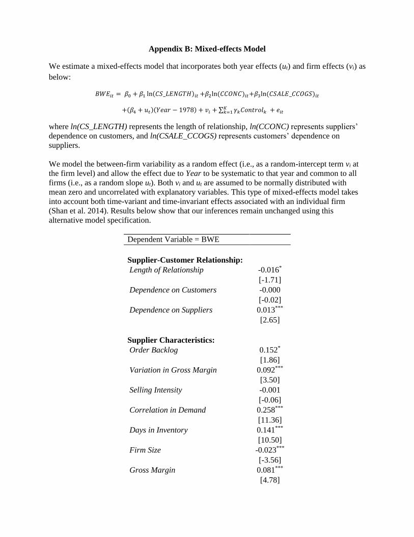
Appendix B: Mixed-effects Model

We estimate a mixed-effects model that incorporates both year effects (ut) and firm effects (vi) as

below:

𝐵𝑊𝐸𝑖𝑡 = 𝛽0 + 𝛽1 ln(𝐶𝑆_𝐿𝐸𝑁𝐺𝑇𝐻)𝑖𝑡 +𝛽2ln (𝐶𝐶𝑂𝑁𝐶)𝑖𝑡+𝛽3ln (𝐶𝑆𝐴𝐿𝐸_𝐶𝐶𝑂𝐺𝑆)𝑖𝑡

+(𝛽4 + 𝑢𝑡)(𝑌𝑒𝑎𝑟 − 1978) + 𝑣𝑖 + ∑ 𝛾𝑘𝐶𝑜𝑛𝑡𝑟𝑜𝑙𝑘𝐾𝑘=1 + 𝑒𝑖𝑡

where ln(CS_LENGTH) represents the length of relationship, ln(CCONC) represents suppliers’

dependence on customers, and ln(CSALE_CCOGS) represents customers’ dependence on

suppliers.

We model the between-firm variability as a random effect (i.e., as a random-intercept term vi at

the firm level) and allow the effect due to Year to be systematic to that year and common to all

firms (i.e., as a random slope ut). Both vi and ut are assumed to be normally distributed with

mean zero and uncorrelated with explanatory variables. This type of mixed-effects model takes

into account both time-variant and time-invariant effects associated with an individual firm

(Shan et al. 2014). Results below show that our inferences remain unchanged using this

alternative model specification.

Dependent Variable = BWE

Supplier-Customer Relationship:

Length of Relationship -0.016*

[-1.71]

Dependence on Customers -0.000

[-0.02]

Dependence on Suppliers 0.013***

[2.65]

Supplier Characteristics:

Order Backlog 0.152*

[1.86]

Variation in Gross Margin 0.092***

[3.50]

Selling Intensity -0.001

[-0.06]

Correlation in Demand 0.258***

[11.36]

Days in Inventory 0.141***

[10.50]

Firm Size -0.023***

[-3.56]

Gross Margin 0.081***

[4.78]

49

Days Payable Outstanding 0.035***

[2.59]

Seasonality in Demand -0.203***

[-24.66]

Year 0.006***

[4.53]

Constant 0.938***

[8.08]

Observations 13,993

Firm and Year Effects Yes

Log Likelihood -16,445.2 ***, **, and * indicate significance level of 1%, 5%, 10%, respectively,

based on two-sided tests.

50

TABLE 1

Sample Selection

This table presents our sample selection procedure. Retail sector includes SIC 5200-5999. Wholesale sector include

SIC 5000-5199. Manufacturing sector includes SIC 2000-3999. Resource extracting sector includes SIC 1000-1400.

Sample Selection Number of

Observations

Annual supplier-customer pairs where both customer and supplier are from

one of the four sectors (retail, wholesale, manufacturing or resource

extracting) and both customer and supplier names can be matched to

corporate names on Compustat

30,279

Less observations where:

Data unavailable to construct the bull whip effect for the supplier 5,377

Data unavailable to construct supplier-customer relationship variables

at the supplier-customer pair level

1,610

Subtotal: Supplier-customer pairs 23,292

Supplier-customer pairs aggregated at the supplier-year level 16,746

Less observations where:

Data unavailable to construct other influential factors including the

control variables

2,753

Total: Supplier-Years 13,993

Number of unique suppliers 2,786

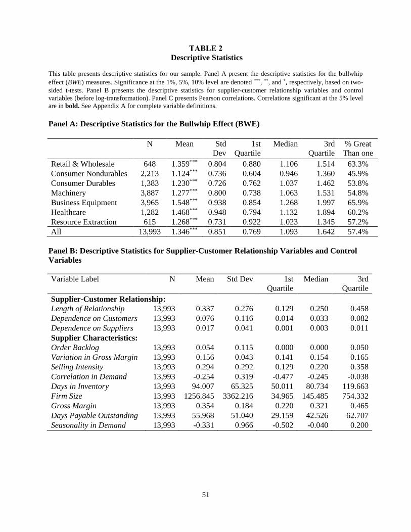
51

TABLE 2

Descriptive Statistics

This table presents descriptive statistics for our sample. Panel A present the descriptive statistics for the bullwhip

effect (BWE) measures. Significance at the 1%, 5%, 10% level are denoted ***, **, and *, respectively, based on two-

sided t-tests. Panel B presents the descriptive statistics for supplier-customer relationship variables and control

variables (before log-transformation). Panel C presents Pearson correlations. Correlations significant at the 5% level

are in bold. See Appendix A for complete variable definitions.

Panel A: Descriptive Statistics for the Bullwhip Effect (BWE)

N Mean Std

Dev

1st

Quartile

Median 3rd

Quartile

% Great

Than one

Retail & Wholesale 648 1.359*** 0.804 0.880 1.106 1.514 63.3%

Consumer Nondurables 2,213 1.124*** 0.736 0.604 0.946 1.360 45.9%

Consumer Durables 1,383 1.230*** 0.726 0.762 1.037 1.462 53.8%

Machinery 3,887 1.277*** 0.800 0.738 1.063 1.531 54.8%

Business Equipment 3,965 1.548*** 0.938 0.854 1.268 1.997 65.9%

Healthcare 1,282 1.468*** 0.948 0.794 1.132 1.894 60.2%

Resource Extraction 615 1.268*** 0.731 0.922 1.023 1.345 57.2%

All 13,993 1.346*** 0.851 0.769 1.093 1.642 57.4%

Panel B: Descriptive Statistics for Supplier-Customer Relationship Variables and Control

Variables

Variable Label

N Mean Std Dev 1st

Quartile

Median 3rd

Quartile


Length of Relationship 13,993 0.337 0.276 0.129 0.250 0.458

Dependence on Customers 13,993 0.076 0.116 0.014 0.033 0.082

Dependence on Suppliers 13,993 0.017 0.041 0.001 0.003 0.011


Order Backlog 13,993 0.054 0.115 0.000 0.000 0.050

Variation in Gross Margin 13,993 0.156 0.043 0.141 0.154 0.165

Selling Intensity 13,993 0.294 0.292 0.129 0.220 0.358

Correlation in Demand 13,993 -0.254 0.319 -0.477 -0.245 -0.038

Days in Inventory 13,993 94.007 65.325 50.011 80.734 119.663

Firm Size 13,993 1256.845 3362.216 34.965 145.485 754.332

Gross Margin 13,993 0.354 0.184 0.220 0.321 0.465

Days Payable Outstanding 13,993 55.968 51.040 29.159 42.526 62.707

Seasonality in Demand 13,993 -0.331 0.966 -0.502 -0.040 0.200

Panel C: Pearson Correlations

(1) (2) (3) (4) (5) (6) (7) (8) (9) (10) (11) (12) (13)

(1) Bullwhip Effect 1

(2) Length of Relationship -0.057 1

(3) Dependence on

Customers 0.001 0.078 1

(4) Dependence on Suppliers 0.018 0.101 0.105

(5) Order Backlog 0.013 0.030 0.001 -0.056 1

(6) Variation in Gross

Margin 0.001 0.058 -0.005 0.053 0.018 1

(7) Selling Intensity 0.096 -0.151 0.028 -0.266 -0.040 -0.231

(8) Correlation in Demand 0.046 -0.017 0.013 0.040 0.019 0.022 -0.037 1

(9) Days in Inventory 0.116 0.010 -0.033 -0.111 0.085 -0.130 0.499 -0.051 1

(10) Firm Size -0.006 -0.043 -0.146 0.515 -0.224 0.019 -0.315 0.043 -0.170 1

(11) Gross Margin 0.103 -0.127 -0.021 -0.090 -0.091 -0.219 0.630 -0.030 0.342 0.014 1

(12) Days Payable

Outstanding 0.081 -0.158 0.067 -0.034 -0.050 -0.143 0.365 0.006 0.137 0.039 0.331 1

(13) Seasonality in Demand -0.194 -0.029 0.036 -0.157 0.067 -0.059 0.178 0.221 0.120 -0.186 0.086 0.082 1

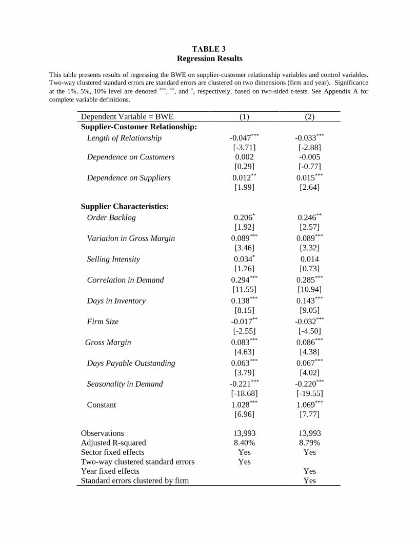
TABLE 3

Regression Results

This table presents results of regressing the BWE on supplier-customer relationship variables and control variables.

Two-way clustered standard errors are standard errors are clustered on two dimensions (firm and year). Significance

at the 1%, 5%, 10% level are denoted ***, **, and *, respectively, based on two-sided t-tests. See Appendix A for

complete variable definitions.

Dependent Variable = BWE (1) (2)


Length of Relationship -0.047*** -0.033***

[-3.71] [-2.88]

Dependence on Customers 0.002 -0.005

[0.29] [-0.77]

Dependence on Suppliers 0.012** 0.015***

[1.99] [2.64]


Order Backlog 0.206* 0.246**

[1.92] [2.57]

Variation in Gross Margin 0.089*** 0.089***

[3.46] [3.32]

Selling Intensity 0.034* 0.014

[1.76] [0.73]

Correlation in Demand 0.294*** 0.285***

[11.55] [10.94]

Days in Inventory 0.138*** 0.143***

[8.15] [9.05]

Firm Size -0.017** -0.032***

[-2.55] [-4.50]

Gross Margin 0.083*** 0.086***

[4.63] [4.38]

Days Payable Outstanding 0.063*** 0.067***

[3.79] [4.02]

Seasonality in Demand -0.221*** -0.220***

[-18.68] [-19.55]

Constant 1.028*** 1.069***

[6.96] [7.77]

Observations 13,993 13,993

Adjusted R-squared 8.40% 8.79%

Sector fixed effects Yes Yes

Two-way clustered standard errors Yes

Year fixed effects Yes

Standard errors clustered by firm Yes

TABLE 4

Subsample Regression Results This table presents results of regressing the BWE on supplier-customer relationship variables and control variables by industry (Panel A) or by sub-period (Panel B).

Two-way clustered standard errors are standard errors are clustered on two dimensions (firm and year). Significance at the 1%, 5%, 10% level are denoted ***, **, and * respectively, based on two-sided t-tests. See Appendix A for complete variable definitions.

Panel A: By Industry

Industries Retail &

Wholesale

Consumer

Nondurables

Consumer

Durables

Machinery Business

Equipment

Healthcare Resource

Extraction


Length of Relationship 0.032 -0.093*** -0.048 -0.038** -0.040* 0.018 -0.040

[0.71] [-2.94] [-1.28] [-2.32] [-1.87] [0.58] [-1.18]

Dependence on Customers -0.025 -0.031 -0.008 -0.011 0.026** 0.006 0.054**

[-1.00] [-0.96] [-0.44] [-1.14] [2.08] [0.37] [2.13]

Dependence on Suppliers -0.005 0.007 0.037** 0.002 0.007 -0.013 -0.018

[-0.24] [0.41] [2.22] [0.19] [0.61] [-0.88] [-0.95]


Order Backlog 0.521 -0.293 0.176 0.440*** -0.105 0.493 -0.369

[0.83] [-1.29] [0.56] [2.80] [-0.56] [0.86] [-1.56]

Variation in Gross Margin 0.149 0.238** 0.050 0.153*** 0.040 0.028 -0.003

[1.09] [2.19] [0.68] [2.94] [0.72] [0.42] [-0.07]

Selling Intensity -0.083 -0.021 0.045 0.004 0.085** -0.076 -0.076

[-0.74] [-0.36] [0.53] [0.14] [2.38] [-1.06] [-1.31]

Correlation in Demand 0.247** 0.169** 0.177** 0.215*** 0.375*** 0.390*** 0.084

[2.04] [2.57] [1.99] [4.01] [9.61] [3.78] [1.02]

Days in Inventory 0.181*** 0.011 0.011 0.160*** 0.139*** 0.157*** 0.185***

[3.52] [0.27] [0.19] [5.53] [4.91] [3.09] [4.72]

Firm Size -0.009 -0.023 -0.061*** -0.031*** 0.002 0.057*** -0.011

[-0.33] [-1.11] [-4.63] [-2.85] [0.16] [3.24] [-0.55]

Gross Margin 0.019 -0.070 0.018 0.017 0.120*** 0.016 0.062

[0.18] [-1.29] [0.26] [0.47] [3.29] [0.17] [1.08]

55

Days Payable Outstanding 0.049 0.093* 0.039 0.083*** -0.012 0.010 0.086**

[0.73] [1.70] [0.94] [3.03] [-0.40] [0.22] [2.24]

Seasonality in Demand -0.213*** -0.164*** -0.165*** -0.193*** -0.279*** -0.276*** -0.200***

[-5.82] [-5.16] [-7.12] [-9.87] [-12.46] [-5.55] [-4.02]

Constant 0.541 1.034*** 1.695*** 0.630*** 1.351*** 0.398 0.254

[0.85] [2.46] [2.97] [2.71] [6.07] [1.06] [0.88]

Observations 648 2,213 1,383 3,887 3,965 1,282 615

Adjusted R-squared 15.5% 5.3% 5.7% 8.3% 8.5% 9.9% 12.5%

Two-way clustered standard

errors

Yes Yes Yes Yes Yes Yes Yes

TABLE 4 CONTINUED

Panel B: By Sub-period

Years 1978-1995 1996-2013


Length of Relationship -0.016 -0.050***

[-0.89] [-3.15]

Dependence on Customers -0.025** 0.008

[-2.47] [0.97]

Dependence on Suppliers 0.018** 0.012*

[2.11] [1.67]


Order Backlog 0.311** 0.216

[2.04] [1.55]

Variation in Gross Margin 0.095*** 0.076**

[2.71] [2.03]

Selling Intensity 0.005 0.016

[0.16] [0.69]


[8.26] [9.31]


[4.42] [8.02]

Firm Size -0.038*** -0.025***

[-3.92] [-3.02]

Gross Margin 0.047** 0.101***

[2.56] [4.29]

Days Payable Outstanding 0.061** 0.068***

[2.27] [3.32]


[-13.42] [-16.08]

Constant 1.164*** 0.935***

[5.53] [4.90]




Two-way clustered standard errors Yes Yes

57

TABLE 5

Regression Results – Nonlinearity

This table presents results of regressing the BWE on linear and squared terms of variables measuring supplier-

customer relationship and control variables. Two-way clustered standard errors are standard errors clustered on two

dimensions (firm and year). Significance at the 1%, 5%, 10% level are denoted ***, **, and * respectively, based on

two-sided t-tests. See Appendix A for complete variable definitions.

Dependent Variable = BWE (1) (2)


Length of Relationship -0.052*** -0.036***

[-3.96] [-2.89]

(Length of Relationship)^2 -0.017 -0.009

[-1.45] [-0.88]

Dependence on Customers 0.005 -0.003

[0.65] [-0.43]

(Dependence on Customers)^2 0.006** 0.006**

[2.21] [1.97]

Dependence on Suppliers 0.013** 0.017***

[2.19] [2.86]

(Dependence on Suppliers)^2 -0.004** -0.005***

[-2.52] [-2.77]


Order Backlog 0.202* 0.241**

[1.87] [2.52]

Variation in Gross Margin 0.087*** 0.087***

[3.46] [3.24]

Selling Intensity 0.036* 0.017

[1.87] [0.90]


[11.39] [10.88]


[8.15] [9.20]

Firm Size -0.019*** -0.034***

[-2.79] [-4.74]

Gross Margin 0.078*** 0.081***

[4.41] [4.13]

Days Payable Outstanding 0.062*** 0.066***

[3.65] [3.98]


[-18.85] [-19.64]

Constant 1.048*** 1.073***

[8.13] [8.54]


58



Two-way clustered standard errors Yes

Year fixed effects Yes

Standard errors clustered by firm Yes

Documents

Supply chain relational capital and the bullwhip effect