Embed Size (px)
Citation preview
SUPPLY NETWORK FORMATION AND FRAGILITY
MATTHEW ELLIOTT, BENJAMIN GOLUB, AND MATTHEW V. LEDUC
Abstract. We model the production of complex goods in a large supply network. Each firm
sources several essential inputs through relationships with other firms. Individual supply relation-
ships are at risk of idiosyncratic failure, which threatens to disrupt production. To protect against
this, firms multisource inputs and strategically invest to make relationships stronger, trading off the
cost of investment against the benefits of increased robustness. A supply network is called fragile
if aggregate output is very sensitive to small aggregate shocks. We show that supply networks of
intermediate productivity are fragile in equilibrium, even though this is always inefficient. The
endogenous configuration of supply networks provides a new channel for the powerful amplification
of shocks.
Date Printed. January 7, 2022.This project has received funding from the European Research Council (ERC) under the European Union’s Horizon2020 research and innovation programme (grant agreement number #757229) and the JM Keynes Fellowships Fund(Elliott); the Joint Center for History and Economics; the Pershing Square Fund for Research on the Foundationsof Human Behavior; and the National Science Foundation under grant SES-1629446 (Golub). We thank seminarparticipants at the 2016 Cambridge Workshop on Networks in Trade and Macroeconomics, Tinbergen Insititute,Monash Symposium on Social and Economic Networks, Cambridge-INET theory workshop (2018), Binoma Workshopon Economics of Networks (2018), Paris School of Economics, Einaudi Institute for Economics and Finance, SeventhEuropean Meeting on Networks, SAET 2019 and the Harvard Workshop on Networks in Macroeconomics. We thankJoey Feffer, Riako Granzier-Nakajima, Yixi Jiang, and Brit Sharoni for excellent research assistance. For helpfulconversations we are grateful to Daron Acemoglu, Nageeb Ali, Pol Antras, David Baqaee, Vasco Carvalho, OlivierCompte, Krishna Dasaratha, Selman Erol, Marcel Fafchamps, Emmanuel Farhi, Alex Frankel, Sanjeev Goyal, PhilippeJehiel, Matthew O. Jackson, Chad Jones, Annie Liang, Eric Maskin, Marc Melitz, Marzena Rostek, Emma Rothschild,Jesse Shapiro, Ludwig Straub, Alireza Tahbaz-Salehi, Larry Samuelson, Andrzej Skrzypacz, Juuso Valimaki andRakesh Vohra. We are grateful to two anonymous referees and the Editor for very helpful comments.
1
1. Introduction
Complex supply networks are a central feature of the modern economy. Consider, for instance,
a product such as an airplane. It consists of multiple parts, each of which is essential for its
production, and many of which are sourced from suppliers. The parts themselves are produced
using multiple inputs, and so on.1 Due to the resulting interdependencies, an idiosyncratic shock
can cause cascading failures and disrupt many firms. We develop a theory in which firms insure
against supply disruptions by strategically forming supply networks, trading off private gains in
the robustness of their production against the cost of maintaining strong supply relationships. Our
main results examine how equilibrium supply networks respond to idiosyncratic and aggregate risk.
We find that, in equilibrium, (i) the economy is robust to idiosyncratic shocks, yet (ii) small shocks
that systemically affect the functioning of supply relationships are massively amplified. Moreover,
(iii) the functioning of many unrelated supply chains is highly correlated, and (iv) the complexity
of production is key to the nature of these effects and the level of aggregate volatility.
Underlying these results is a discontinuous phase transition in the structure of production net-
works that arises due to production being complex—reliant on multiple inputs at many stages.
Thus, a theoretical contribution of our work is the study of novel equilibrium fragilities in the
strategic formation of large networks, and new methods for analyzing them.
Our analysis is built on a model of interfirm sourcing relationships and their disruption by
shocks. We now motivate our study of these phenomena with some examples. Firms often rely on
particular suppliers to deliver customized inputs. For instance, Rolls-Royce designed and developed
its Trent 900 engine for the Airbus A380; Airbus could not just buy the engine it requires off-the-
shelf. Such inputs are tailored to meet the customer’s specifications, and there are often only a
few potential suppliers that a given firm contracts with. Thus, a particular airplane producer is
exposed not just to shocks in the overall availability of each needed input, but also to idiosyncratic
shocks in the operation of the few particular supply relationships it has formed. Examples of
such idiosyncratic shocks include a delay in shipment, a fire at a factory, a misunderstanding by a
supplier that delivers an unsuitable component, or a strike by workers. As we have noted, many
of a given firm’s suppliers themselves will be in a similar position, relying on customized inputs,
and so idiosyncratic disruptions to individual relationships and production processes somewhere in
a network can have far-reaching effects, causing damage that cascades through the supply chain
and affects many downstream firms.2 On the other hand, many firms multisource key inputs to
reduce their dependency on any one supplier and so idiosyncratic disruptions may not cause much
reduction in output at all.
Even the basic properties of such complex supply networks are not well-understood. To articu-
late this, we describe a simple model capturing key aspects of the above examples. There are many
products (e.g., airplanes, engines, etc.). Each has many differentiated varieties, produced by small,
1For example, an Airbus A380 has millions of parts produced by more than a thousand companies (Slutsken, 2018).In addition to the physical components involved, many steps of production require specific contracts and relationshipswith logistics firms, business services, etc. to function properly.2Kremer (1993) is a seminal study of some theoretical aspects of such propagation. Carvalho et al. (2020) empiricallystudy how shocks caused by the Great East Japan Earthquake of 2011 propagated through supply networks tolocations far from the initial disruption. In Section 6, we discuss further evidence that such disruptions are practicallyimportant, and can be very damaging to particular firms.

2 MATTHEW ELLIOTT, BENJAMIN GOLUB, AND MATTHEW V. LEDUC
specialized firms. A given product has a set of customized inputs that must be sourced via sup-
ply relationships and are essential to its production—e.g., an airplane requires engines, navigation
systems, etc. To source these specific, compatible, varieties firms may have several substitutable
sourcing options (i.e., they multisource). Each of a firm’s potential supply relationships may oper-
ate successfully or not: e.g., one engine manufacturer’s delivery may be delayed by a strike, while
another is able to deliver normally. In order for a firm to be functional, it must have at least one
operating supply relationship to a firm producing each of its essential inputs. To be functional,
these producers must in turn satisfy the same condition, and so on—until a point in the supply
chain where no customized inputs are required. Our modelling of which supply relationships work
is simple: independently, each relationship operates successfully with a probability called the re-
lationship strength.3 This probability represents the chance of avoiding logistical disruptions and
failures of contracts in any specific relationship. Given a realization of operating relationships, the
firms that are able to produce purchase their required inputs and then sell their products to other
firms as well as to consumers. Social welfare is increasing in the number of firms able to produce.
Firms make profits from production.
Let us, to begin with, take relationship strength to be exogenous and symmetric across the supply
network, and examine aggregate output as we vary this parameter. The key parameters other than
relationship strength for describing the mechanics of a supply network are (i) the number of distinct
inputs required in each production process; (ii) the number of potential suppliers of each input;
and (iii) the depth of supply chains, i.e., the number of steps of specialized sourcing. The first and
third dimensions capture the complexity of production, while the second captures the availability
of multisourcing. In our model there is a continuum of firms and the fraction of firms functioning
is deterministic.4 This fraction is our main outcome of interest, and we call it the reliability of
the supply network. Our first main result concerns a distinctive form of sensitivity that can arise
in such networks—what we call a precipice. Suppose production is complex—that is, that most
firms have multiple essential inputs they need to source, and supply networks are deep, meaning
that many steps of such production are needed. We find that there is a discontinuity in reliability
as we vary relationship strength, holding all else fixed. When relationship strength falls below a
certain threshold (defining the precipice), production drops discontinuously. Thus, if relationship
strengths happen to be close to the precipice, a small, systemic, negative shock to relationship
strengths is amplified arbitrarily strongly, leading to severe economic damage. We also show that a
social planner choosing a level of investments in relationship strengths to maximize welfare would
never choose a level such that the supply network is on a precipice.
We give a few practical examples of systemic shocks to relationship strengths. Suppose, first, that
the institutions that help uphold contracts and facilitate business transactions suddenly decline in
quality, for example due to a political shock. Each supply relationship then becomes more prone
to the idiosyncratic disruptions discussed above.5 Even if the damage to any single relationship
3Though the modeling of basic shocks is independent, the interdependence between firms and their suppliers makesfailures correlated between firms that (directly or indirectly) transact with each other.4This is by a standard diversification argument. There are enough firms and supply chains operating that none ofthem is systemically important. On the complementary issue of when individual firms can be systemically important,see Gabaix (2011) and the large ensuing literature.5Blanchard and Kremer (1997) present evidence that the former Soviet Union suffered a large shock of this kind whenit transitioned to a market-based economy.
3
is small (e.g., because usually contracts function without enforcement being relevant), our results
show that such a shock can cause widespread disruptions throughout the supply network. For a
second concrete interpretation of the kinds of aggregate shocks we have in mind, consider a small
shock to the availability of credit for businesses in the supply network. The shock matters for
firms that are on the margin between getting and not getting credit that is essential for them to
deliver on a commitment. The effect of such a credit shock can be modeled as any given supply
relationship being slightly less likely to function (depending on ex ante uncertain realizations of
whether a firm is on the relevant margin). Third, during the Covid-19 crisis, there has been much
uncertainty about how different supply relationships might be affected, and this can be modeled as
a systemic decrease in the probability that suppliers are able to deliver the inputs required from
them.
The first result just discussed on exogenous relationship strengths shows that, starting at certain
strength levels, supply network functioning can be very sensitive to slight shocks to strengths.
However, relationship strengths are strategic choices, and the endogenous determination of these
is in fact our main focus. Our question is whether a supply network will be near a precipice
when relationship strengths are determined by equilibrium choices rather than exogenously or by
a planner. Since production is risky, an optimizing firm will strategically choose its relationship
strength to manage the risk of its production being disrupted. By investing more, a firm can
increase the probability that one of its potential suppliers for each of its essential inputs is able to
supply it, hence allowing the firm to produce its output and make profits. Maintaining multiple
relationships that facilitate production and provide backup in case of disruption is costly. Firms
trade off these costs against the benefits of increased robustness.6 In our model, firms choose a level
of costly investment toward making their supply relationships stronger—i.e., likelier to operate.7
Our main findings give conditions for equilibrium relationship strength levels to put the supply
network on the precipice, and show that the precipice is not a knife-edge outcome. Indeed, we
characterize a positive-measure set of parameters (governing the profits of production and the costs
of forming relationships) for which the equilibrium supply network is on the precipice. The fragility
that a supply network experiences in this regime is highly inefficient: a social planner would never
put a supply network on the precipice for the same parameters. As supply networks become large
and decentralized one might think that the impact of uncertainty on the probability of successful
production would be smoothed by firms’ endogenous investments to protect against shocks, and by
averaging outcomes across a continuum population. We find the opposite: in equilibrium, there is a
very sharp sensitivity of aggregate productivity to relationship strength. This is in contrast to many
standard production network models, where the aggregate production function is not too sensitive
to small shocks at any outcome. The novelty of our framework comes from the combination of
two features of production functions that are essential for our results. The first is complexity: The
supply networks we study are many layers deep and firms must source multiple essential inputs
6Strategic responses to risk in networks is a topic that has attracted considerable attention recently. See, for instance,Bimpikis, Candogan, and Ehsani (2019a), Blume, Easley, Kleinberg, Kleinberg, and Tardos (2011), Talamas andVohra (2020), and Erol and Vohra (2018), Amelkin and Vohra (2019), and Acemoglu and Tahbaz-Salehi (2020). Onthe practical importance of the strength of contracts in supply relationships, see, among others, Antras (2005) andAcemoglu, Antras, and Helpman (2007).7This can be interpreted in two ways: (1) investment on the intensive margin, e.g. to anticipate and counteract risksor improve contracts; (2) on the extensive margin, to find more partners out of a set of potential ones.
4 MATTHEW ELLIOTT, BENJAMIN GOLUB, AND MATTHEW V. LEDUC
that cannot be purchased off-the-shelf. The second is the presence of idiosyncratic disruptions to
supply. Jointly, these phenomena create the possibility of precipices, which underlie our analysis.
More specifically, our main results concern whether the supply network is on a precipice as we
vary an aggregate productivity parameter.8 Depending on the value of this parameter, the supply
network in equilibrium can end up in one of three configurations: (i) a noncritical equilibrium
where the equilibrium investment is enough to keep relationship strength away from the precipice;
(ii) a critical equilibrium where equilibrium relationship strength is on the precipice; and (iii) an
unproductive equilibrium where positive investment cannot be sustained. These regimes are ordered.
As the productivity of the supply network decreases from a high to a low level, the regimes occur
in the order just given. Each regime occurs for a positive interval of values of the parameter.
Equivalently, for an economy consisting of many disjoint supply networks distributed with full
support over the parameter space, a positive measure of them will be in the fragile regime, and
these will collapse if relationship quality is shocked throughout the economy.
Our analysis makes a conceptual, modeling, and technical contribution to the theory of economic
networks. First, we introduce percolation analysis (i.e., disabling some links at random) to an oth-
erwise standard network model of complex production—with complex meaning that each firm must
source multiple inputs through customized relationships.9 That combination leads to the finding
that under natural assumptions, random failures in a production network result in a discontinuous
phase transition, where aggregate functionality abruptly disappears when relationship strengths
cross a critical threshold. Simple production, which does not require risky sourcing of multiple
inputs, is not susceptible to this fragility. Second, as a modeling contribution, we demonstrate the
tractability of studying equilibrium investments in links (more precisely, investments in the proba-
bility that links are operational) in such a setting. By defining a suitable model with a continuous
investment choice and a continuum of nodes, investment problems are characterized by relatively
tractable first-order conditions, because firms are able to average over the randomness in network
realizations. We expect the modeling devices we develop to have other applications. Finally, using
our equilibrium conditions to deduce the ordering of regimes discussed above requires developing
some new techniques for the analysis of large network formation games.10 For example, a crucial
step in our main results depends on showing that firms’ investments in network formation are lo-
cally strategic substitutes at the equilibrium investment levels, which depends on subtle properties
of equilibrium network structure and incentives that we characterize.
We explore some extensions and implications of our modeling. First, we examine robustness on
a number of dimensions. We discuss why the basic insights about fragility extend to alternative
specifications of shocks and investment in relationships. Perhaps our most important robustness
check concerns relaxing certain symmetries of the supply network that we use to simplify our main
analysis. We study how fragility manifests with firm heterogeneity. In particular, we show that
precipices continue to obtain in presence of rich heterogeneity across multiple dimensions (number
of inputs required, multisourcing possibilities, directed multisourcing efforts, profitability, etc.).
One important additional implication of our heterogeneity analysis is that a supply network is only
8This parameter can be interpreted as a measure of productivity relative to the costs of maintaining relationships.9A recent model motivated by some of the same questions is Acemoglu and Tahbaz-Salehi (2020), where each nodein a production network relies on one failure-prone custom supplier. In Section 7, we discuss related models oninformation sharing, financial contagion, and other settings.10This differs from and complements the use of graphons in Erol, Parise, and Teytelboym (2020).
5
as strong as its weakest links: as one product enters the fragile regime, all products that depend
on it directly or indirectly are simultaneously pushed into the fragile regime. Second, we interpret
our main results in terms of the short- and medium-run resilience of a supply network to shocks,
and consider whether the fragility we identify can be ameliorated by natural policy interventions.
Third, we show how the supply networks we have studied can be embedded in a larger economy
with intersectoral linkages that do not rely on specific sourcing. Our model yields a new channel for
the propagation of shocks across sectors, and their stark amplification. Fourth, while the focus of
our analysis is on linking complex supply networks to aggregate volatility, we also discuss how the
model can provide a perspective on some stylized facts concerning industrial development (Section
8.4). After presenting our results, in Sections 6 and 7 we discuss in detail how they fit into the
most closely related literatures.
2. Model: The supply network
Our main object of study is a network whose nodes are a continuum of small firms producing
differentiated products. These are connected to their suppliers by a network of potential supply
relationships, a random subset of which are realized as operational for sourcing.
An outcome of central interest is the set of firms that is functional—i.e., capable of producing.
The measure of functional firms will be the key quantity of interest in our model, determining
welfare and incentives to invest to form the network, which we introduce in Section 4. The purpose
of this section is to set up the basic structure of the production network and define the set of
functional firms.
2.1. Nodes: Varieties of products. There is a finite set I of products. For each product i ∈ I,
there is a continuum Vi of varieties of i, with a typical variety v being an ordered pair v = (i, f),
where f ∈ Fi ⊆ R is a variety index; we take Fi = [0, 1/|I|] for all i, so that the total mass of firms
(and of varieties) in the supply network is 1. Let V =⋃i∈I Vi be the union of all the varieties.
These are the nodes in our supply network. Each is associated with a small firm producing the
corresponding variety.
2.2. Links: Potential and realized supply relationships. First, for each product i ∈ I there
is a set of required inputs I(i) ⊆ I. Second, each variety v ∈ V is associated with a supply chain
depth d(v) ∈ Z+ that specifies how many steps of customized, specifically sourced production are
required to produce v, with varieties of larger depth requiring more steps. Different varieties of the
same product can have different depths. The measure of varieties with any depth d ≥ 0 is denoted
by µ(d).
Consider any variety v ∈ Vi. For each j ∈ I(i) (i.e., each required input) the variety v has a set
of potential suppliers, PSj(v) ⊆ Vj and a random subset of realized suppliers Sj(v) ⊆ PSj(v).
First consider the varieties v ∈ V such that d(v) = 0. Specialized sourcing of inputs is not
required for these varieties, and they operate without disruption. Thus, in this case, we take
Sj(v) = Vj for each j ∈ I(i).
Next, consider any variety v ∈ Vi that has depth d(v) > 0. For each j ∈ I(i), the set PSj(v) is a
finite set of distinct varieties v′ ∈ Vj with each such v′ having depth d(v′) = d(v)−1. The identities
of these suppliers are independent draws from the set of varieties v′ such that d(v′) = d(v)− 1 (i.e.,
6 MATTHEW ELLIOTT, BENJAMIN GOLUB, AND MATTHEW V. LEDUC
the set of varieties of compatible depth).11 Specialized sourcing requirements represent the need
for a customized input, the procurement of which is facilitated by relational contracts.
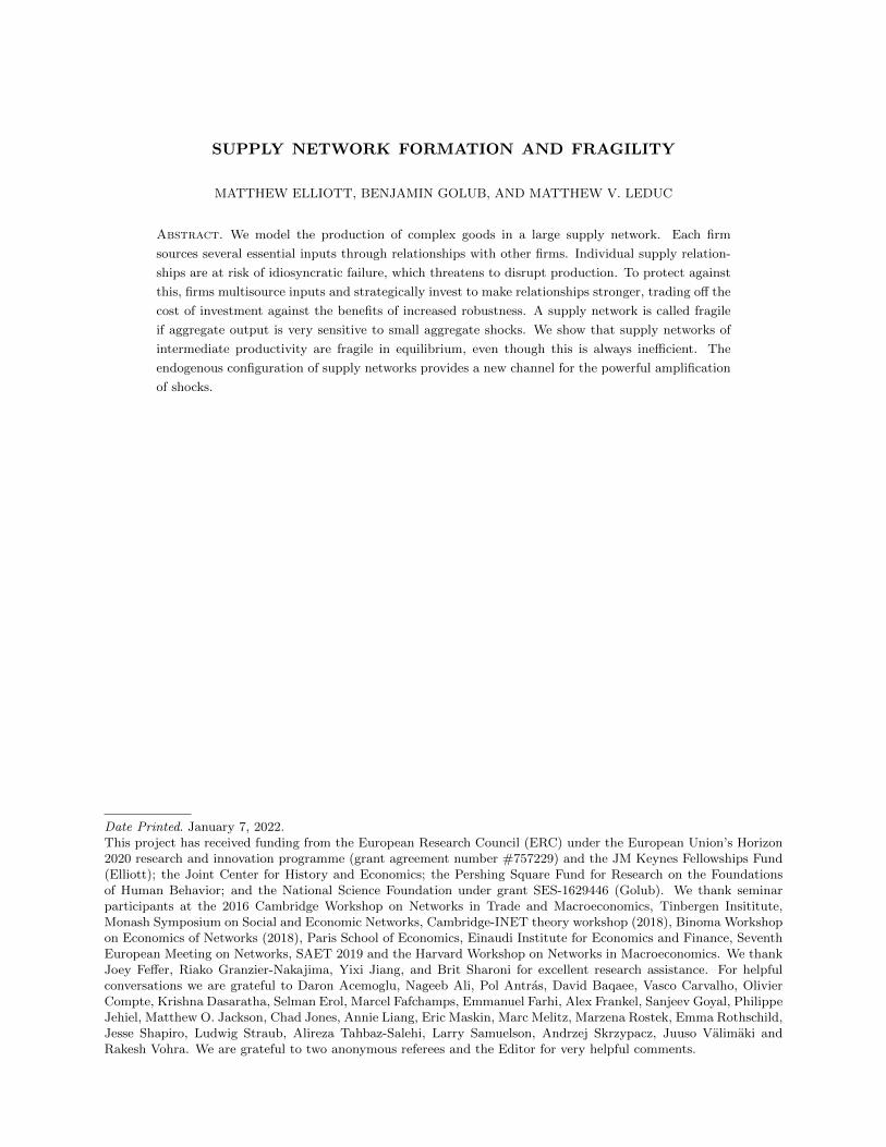
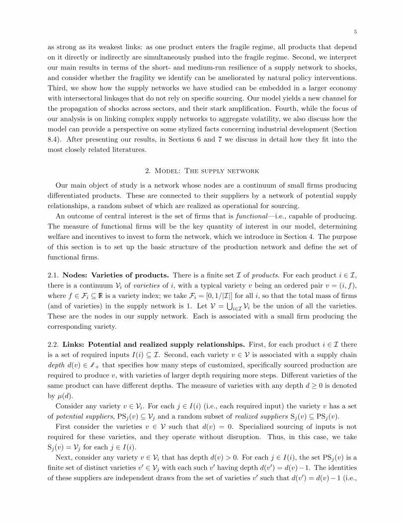
a1
b1 b2 c2c1
d1 d2 c3 c4 d3 d4 c5 c6 a5a4e4e3a3a2e2e1
Figure 1. Here we consider a potential supply network for variety (a, 1) with underlying productsI = {a, b, c, d, e}; the relevant input requirements are apparent from the illustration. Each varietyrequires two distinct inputs. When these inputs must be specifically sourced, there is an edge fromthe sourcing variety to its potential supplier. We abbreviate (a, 1) as a1 (and similarly for othervarieties). Here variety a1 has depth d(a1) = 2. Varieties higher up are upstream of a1, and theirdepths are smaller. Orders or sourcing attempts go in the direction of the arrows, and products aredelivered in the opposite direction, downstream.
Each sourcing relationship between v and a variety v′ ∈ PSj(v) is operational or not—a binary
random outcome. For every v ∈ V, there is a parameter xv, called relationship strength (for now
exogenous) which is the probability that any relationship v has with its suppliers is operational.
All realizations of relationship operation are independent. The set of actual suppliers Sj(v) is then
obtained by including each potential supplier in PSj(v) independently with probability xv. Whereas
the potential supply relationships define compatibilities, the realized supply network identifies which
links are actually available for sourcing. The stochastic nature of availability arises, e.g., from
uncertainty in delivery of orders, miscommunications about specifications, etc.12
We define two random networks on the set V of nodes. In the potential supply network G, each v
has links directed to all its potential suppliers v′ ∈⋃j∈I(i) PSj(v). (See Figure 1 for an illustration.)
In the realized supply network G′, each v has only the operational subset of links, to the realized
suppliers: v′ ∈⋃j∈I(i) Sj(v). See the links in Figure 2 for an illustration of the subset of supply
relationships that are operational.
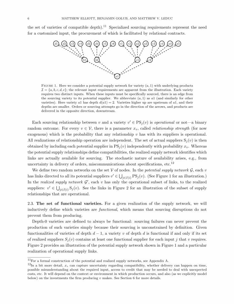
2.3. The set of functional varieties. For a given realization of the supply network, we will
inductively define which varieties are functional, which means that sourcing disruptions do not
prevent them from producing.
Depth-0 varieties are defined to always be functional: sourcing failures can never prevent the
production of such varieties simply because their sourcing is unconstrained by definition. Given
functionalities of varieties of depth d − 1, a variety v of depth d is functional if and only if its set
of realized suppliers Sj(v) contains at least one functional supplier for each input j that v requires.
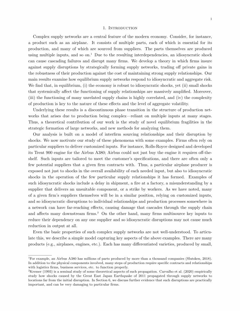
Figure 2 provides an illustration of the potential supply network shown in Figure 1 and a particular
realization of operational supply links.
11For a formal construction of the potential and realized supply networks, see Appendix A.12In a bit more detail, xv can capture uncertainty regarding compatibility, whether delivery can happen on time,possible misunderstanding about the required input, access to credit that may be needed to deal with unexpectedcosts, etc. It will depend on the context or environment in which production occurs, and also (as we explicitly modelbelow) on the investments the firm producing v makes. See Section 6 for more details.
7
a1
b1 b2 c2c1b1
d1 d2 c3 c4 d3 d4 c5 c6 a5a4e4e3a3a2e2e1
(A) Step 1: Assigning functionalities for depth-1 varieties.
b1 c2b2 c2
a1
c1b1
d1 d2 c3 c4 d3 d4 c5 c6 a5a4e4e3a3a2e2e1
(B) Step 2: Assigning functionalities of depth-2 varieties.
Figure 2. An illustration for determining the set of functional varieties given a realized supplynetwork. Functional varieties are represented by green circles, while non-functional ones are pinksquares. Varieties that have not yet been assigned to be functional or not are white circles. Varietiesof depth 0 are always functional. Panel (A) assigns functionalities to varieties of depth 1. Panel(B) assigns functionalities to varieties of depth 2, making a1 nonfunctional.
We let V ′ denote the (random) set of functional varieties, and V ′i denote the set of functional
varieties in product i.
3. Reliability with exogenous relationship strengths
We present our main findings in regular supply networks. These are defined by two main sym-
metries. First, the number of essential inputs is |I(i)| = m for each product i. Second, each variety
of depth d > 0 has n potential suppliers for each input—i.e. |PSj(v)| = n whenever j is one of the
required inputs for variety v. Networks with these homogeneous structures are depicted in Figures
1 and 2. In this section, we posit that relationship strengths are given by xv = x, the same number
for each v, and this x is exogenous.13
It will be important to characterize how the measure of functional firms V ′ varies with relationship
strength x. Denote by ρ(x, d) the probability that an arbitrary variety of depth d is functional when
relationship strength is x. Zero-depth varieties are functional by our assumption that they do not
need any specialized inputs: ρ(x, 0) = 1. By symmetry of the supply tree, the probability ρ(x, d)
does indeed only depend on x and d (and we calculate it explicitly below in Section 3.1.1). The
probability that a variety selected uniformly at random is functional is called the reliability of the
supply network. Since it depends on the distribution of depths µ, we denote this by ρ(x, µ) and
define it as
ρ(x, µ) =∞∑d=0
µ(d)ρ(x, d). (1)
13We endogenize relationship strengths in the next section, and we relax the symmetry assumptions in Section 6.3.2.
8 MATTHEW ELLIOTT, BENJAMIN GOLUB, AND MATTHEW V. LEDUC
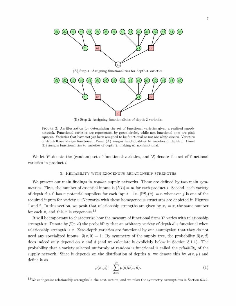
𝑥
1
1(a)
𝜌(𝑥)
𝑥
1
1𝑥𝑐𝑟𝑖𝑡
(b)
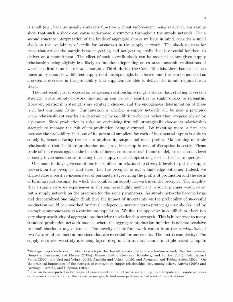
Figure 3. Panel (A) shows how reliability varies with relationship strength x for a particular τ .Panel (B) depicts a correspondence that is the limit of the graphs ρ(x, µτ ) as τ tends to infinity.
Deep supply networks: Taking limits. A focus throughout will be the case where a typical variety
has large depth.14 We thus introduce a notation for asymptotics: we fix a sequence (µτ )∞τ=1 of
distributions, τ is a parameter we will take to be large. We assume µτ places probability at least
1 − 1τ on [cτ,∞) for some c > 0.15 For instance, we can take µτ to be the geometric distribution
with mean τ (in which case τ has an exact interpretation as average depth). For large τ , if inputs
are single-sourced (n = 1) and links fail with positive probability, there will only be a very remote
probability of successful production. We therefore restrict attention to the case of multisourcing
(n ≥ 2).
3.1. A discontinuity in reliability. A key implication of the model is the shape of the aggregate
reliability function as we vary x. As we will see in the next section, this function is closely linked
to the aggregate production function of the supply network, and thus its shape underlies many of
our results. Our first result characterizes important properties of this shape.
Proposition 1. Fix any n ≥ 2 and m ≥ 2. Then there exist positive numbers xcrit, rcrit > 0 such
that,
(i) if x < xcrit, we have that ρ(x, µτ )→ 0 as τ →∞. That is, reliability converges to 0.
(ii) if x > xcrit, then, for all large enough τ , we have ρ(x, µτ ) > rcrit. That is, reliability remains
bounded away from 0.
In Figure 3(a) we plot the reliability function ρ(x, µτ ) for a fixed finite value of τ against the
probability x of each relationship being operational. One can see a sharp transition in relationship
strength x. This can be seen more sharply in Figure 3(b), where we plot the limit of the graph shown
in (a) as τ →∞. We use the m = n = 2 case here as in our illustrations above. There is a critical
value of relationship strength, which we call xcrit, such that the probability of successful production
is 0 when x < xcrit, but then increases sharply to more than 70% for all x > xcrit. Moreover, the
14Supplementary Appendix SA4 investigates how reliability varies with investment in production trees with boundeddepth.15Note that this means varieties of low depth have many incoming edges in the potential supply network, since thereare relatively few of them, but they make up a relatively large number of the nodes in a typical production tree.
9
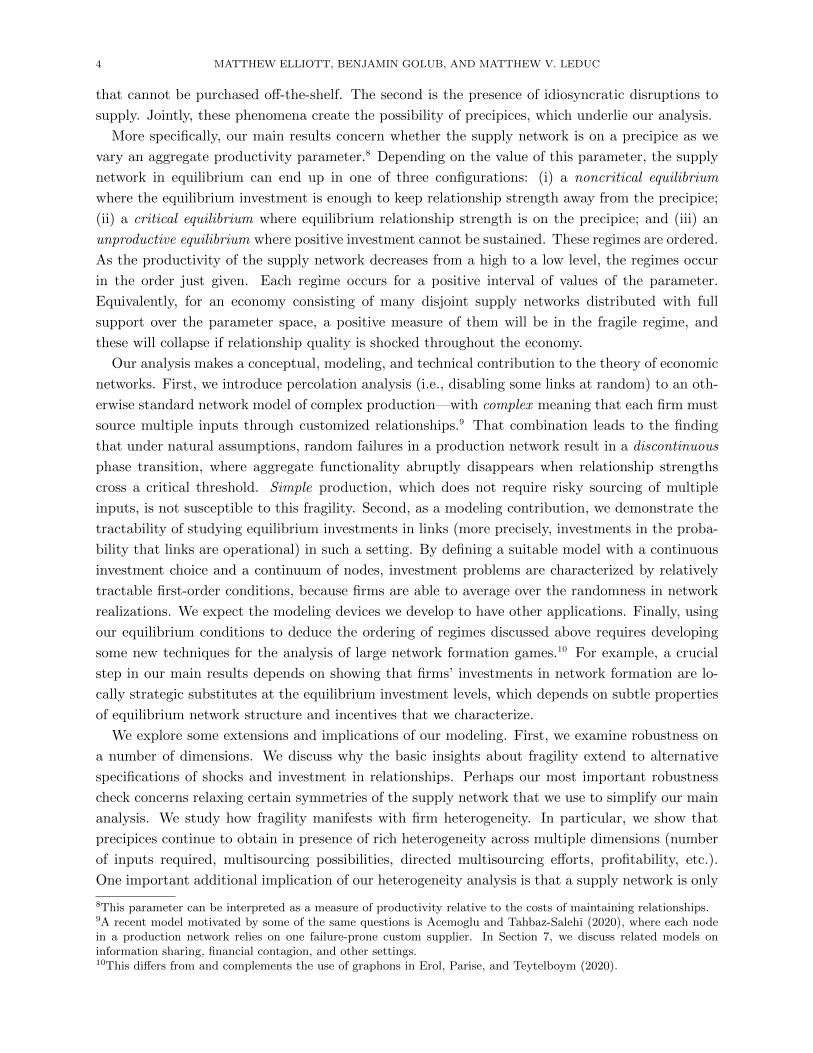
Prob
. buy
er fu
nctio
nal,
Prob. each supplier functional, r
𝑥𝑥 = 0.5
𝑥𝑥 = 0.65
(a)
Prob
. buy
er fu
nctio
nal,
Prob. each supplier functional, r
�𝜌𝜌(𝑥𝑥, 0)
�𝜌𝜌(𝑥𝑥, 1)
�𝜌𝜌(𝑥𝑥, 2)�𝜌𝜌(𝑥𝑥, 3)
�𝜌𝜌(𝑥𝑥, 4)
(b)
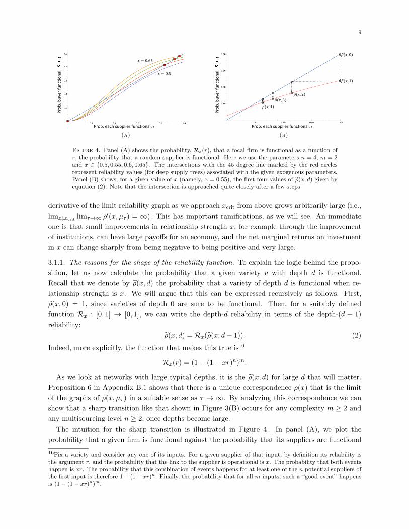
Figure 4. Panel (A) shows the probability, Rx(r), that a focal firm is functional as a function ofr, the probability that a random supplier is functional. Here we use the parameters n = 4, m = 2and x ∈ {0.5, 0.55, 0.6, 0.65}. The intersections with the 45 degree line marked by the red circlesrepresent reliability values (for deep supply trees) associated with the given exogenous parameters.Panel (B) shows, for a given value of x (namely, x = 0.55), the first four values of ρ(x, d) given byequation (2). Note that the intersection is approached quite closely after a few steps.
derivative of the limit reliability graph as we approach xcrit from above grows arbitrarily large (i.e.,
limx↓xcrit limτ→∞ ρ′(x, µτ ) = ∞). This has important ramifications, as we will see. An immediate
one is that small improvements in relationship strength x, for example through the improvement
of institutions, can have large payoffs for an economy, and the net marginal returns on investment
in x can change sharply from being negative to being positive and very large.
3.1.1. The reasons for the shape of the reliability function. To explain the logic behind the propo-
sition, let us now calculate the probability that a given variety v with depth d is functional.
Recall that we denote by ρ(x, d) the probability that a variety of depth d is functional when re-
lationship strength is x. We will argue that this can be expressed recursively as follows. First,
ρ(x, 0) = 1, since varieties of depth 0 are sure to be functional. Then, for a suitably defined
function Rx : [0, 1] → [0, 1], we can write the depth-d reliability in terms of the depth-(d − 1)
reliability:
ρ(x, d) = Rx(ρ(x; d− 1)). (2)
Indeed, more explicitly, the function that makes this true is16
Rx(r) = (1− (1− xr)n)m.
As we look at networks with large typical depths, it is the ρ(x, d) for large d that will matter.
Proposition 6 in Appendix B.1 shows that there is a unique correspondence ρ(x) that is the limit
of the graphs of ρ(x, µτ ) in a suitable sense as τ → ∞. By analyzing this correspondence we can
show that a sharp transition like that shown in Figure 3(B) occurs for any complexity m ≥ 2 and
any multisourcing level n ≥ 2, once depths become large.
The intuition for the sharp transition is illustrated in Figure 4. In panel (A), we plot the
probability that a given firm is functional against the probability that its suppliers are functional
16Fix a variety and consider any one of its inputs. For a given supplier of that input, by definition its reliability isthe argument r, and the probability that the link to the supplier is operational is x. The probability that both eventshappen is xr. The probability that this combination of events happens for at least one of the n potential suppliers ofthe first input is therefore 1− (1− xr)n. Finally, the probability that for all m inputs, such a “good event” happensis (1− (1− xr)n)m.
10 MATTHEW ELLIOTT, BENJAMIN GOLUB, AND MATTHEW V. LEDUC
(which is taken to be common across the suppliers, and denoted by r). The curve Rx(r) is shown
for several values of x. In panel (B), one of these Rx(r) curves is sketched (note the change in axes)
along with the 45-degree line; the figure shows that if we repeatedly apply formula (2) starting
with ρ(x, 0) = 1, we get a a sequence of ρ(x, d) converging to the largest fixed point of Rx(r). As
supply networks become deep, a firm and its suppliers occupy essentially equivalent positions, so
it is natural that the limit probability of being functional for large-depth firms is equal to such a
fixed point. The reliability levels r that are fixed points of the function Rx(r) in equation (2) are
given by its intersections with the 45-degree line, illustrated in panel (A) for several values of x
(each corresponding to one of the curves). We will now examine how the largest such intersection
depends on x. For high enough x, the function Rx(r) has a fixed point with r > 0. When x is below
a certain critical value xcrit, the graph of Rx has no nonzero intersection with the 45-degree line and
so the limit of ρ(x, d) as d→∞ is 0. Crucially, the largest fixed point of Rx(r) does not decrease
continuously down to 0 as we lower x. Instead, it drops down discontinuously when x decreases
past xcrit—defined as the (positive) value of x where there is a point of tangency between Rx(r) and
the 45-degree line. At this point, the largest r solving r = Rx(r) jumps down discontinuously from
the r corresponding to this point of tangency to 0. This is the discontinuous “precipice” drop. As
we explain in Section 6.1.1 where we contrast complex production (m > 1) with simple production
(m = 1), the convex-then-concave shape of the Rx curve is essential for creating a precipice.
3.1.2. Comparative statics of the reliability function. Some straightforward comparative statics can
be deduced from what we have said. If n (multisourcing) increases while all other parameters are
held fixed, then one can check that Rx (as illustrated in Figure 4(A)) increases pointwise on (0, 1),
and this implies that all the ρ(x, d) increase. It follows that the ρ curve moves upward, and the
discontinuity occurs at a lower value of x.
Similarly, when m (complexity) increases, the Rx curve decreases pointwise, implying that all
the ρ(x, d) decrease. It follows that the ρ curve moves downward, and the discontinuity occurs at
a higher value of x.
4. Supply networks with endogenous relationship strength
In this section, we study the endogenous determination of relationship strength. We first study
a planner’s problem—choosing an optimal value of strength for all relationships. We then turn to
a decentralized problem in which firms invest in their own relationship strengths. Throughout, we
focus on symmetric outcomes.
Our main results show that while investments that put the supply network on the precipice are
very inefficient, they need not be knife-edge or even unlikely outcomes in equilibrium.
To connect the graph-theoretic notion of reliability in the previous section with economic out-
comes, we introduce a relationship between reliability and output. In particular, we posit that
there is a function Y such that Y (V ′) is the (expected) aggregate gross output associated with a
given set V ′ of functional firms. We assume that it satisfies the following assumption:
Property A. In a regular supply network, Y (V ′) = h(ρ(x, µ)), where h : [0, 1] → R is a strictly
increasing, concave function with bounded and continuous derivative. Moreover, h(0) = 0.
11
In Appendix C, we provide a microfoundation for this assumption: we define a standard produc-
tion network model on top of the supply network, being explicit about production functions and
markets at the micro level. There, we show that aggregate output satisfies Property A. However,
our main results—about efficient and equilibrium networks—do not rely on any details of the mi-
crofoundations. Instead, they rely only on assumptions about benefits and costs of production that
we bring out into named properties.
Property A sets the stage for our study of the planner’s problem.
4.1. A planner’s problem. We study a planner who chooses a global x that determines the
values of all relationship strengths, xv = x. This can be interpreted as investing in the quality of
institutions, at a cost that we will introduce below. As stipulated in Property A, the gross output
of the supply network is an increasing function of reliability, Y (V ′) = h(ρ(x, µ)), where reliability ρ
depends on the symmetric level of relationship strengths x and depth distribution µ. The planner’s
cost of a given choice of x enters through subtracting a quantity 1κcP (x) of output, where κ is a
strictly positive parameter and cP : [0, 1] → R is a fixed function. Higher values of κ have the
interpretation that they shift down the costs of obtaining a given level of relationship strengths,
and hence a given level of gross output. The planner seeks to maximize expected net aggregate
output by choosing relationship strengths x, and hence solves the planner’s problem
maxx∈[0,1]
h(ρ(x, µ))− 1
κcP (x). (3)
We make the following assumption concerning cP (x):
Property B. The function cP : [0, 1] → R is continuously differentiable and weakly convex, with
cP (0) = 0, cP (xcrit) > 0, c′P (0) = 0, and limx→1 c′P (x) =∞.
Substantively, the conditions in this property entail that there are increasing marginal social costs
of relationship strength and achieving the critical level of reliability requires a positive investment.
The Inada conditions on derivatives ensure good behavior of optima.
Define the correspondence
xSP (κ, µ) := argmaxx∈[0,1]
h(ρ(x, µ))− 1
κcP (x).
This gives the values of x that solve the social planner’s problem for a given κ and distribution of
supply chain depths µ. As elsewhere, we consider a sequence (µτ )∞τ=1 of depth distributions, where
µτ places mass at least 1− 1τ on [τ,∞).
Proposition 2. Fix any n ≥ 2 and m ≥ 2. Then there exists a number κcrit > 0 such that, for
some ε > 0, the following statements hold for all large enough τ :
(i) for all κ < κcrit, all values of xSP (κ, µτ ) are at most xcrit − ε, have cost less than ε, and
yield reliability less than ε;
(ii) for all κ > κcrit, all values of xSP (κ, µτ ) are at least xcrit + ε and yield reliability at least
rcrit + ε;
(iii) for κ = κcrit, all values of xSP (κ, µτ ) are outside the interval [xcrit−ε, xcrit+ε] and reliability
is outside the interval [ε, rcrit + ε].

12 MATTHEW ELLIOTT, BENJAMIN GOLUB, AND MATTHEW V. LEDUC
The first part of Proposition 2 says that when κ is sufficiently low, it is too costly for the social
planner to invest anything in the quality of institutions, and hence reliability is very low. As κ
crosses a threshold κcrit, it first becomes optimal to invest in institutional quality. At this threshold,
the social planner’s investment increases discontinuously. Moreover, it immediately increases to a
level strictly above xcrit; and for all larger κ all solutions stay above xcrit.
It is worth emphasizing that the planner never chooses to invest near the critical level xcrit. The
reason is as follows: sufficiently close to x = xcrit, the marginal social benefits of investing grow
arbitrarily large in the limit as τ gets large while marginal costs at xcrit are bounded, and so the
social planner can always do better by increasing investment at least a little. In contrast, in Section
5 we will see that individual investment choices can put the supply network on the precipice in
equilibrium, and this is not a knife-edge scenario.
4.2. Decentralized investment in relationship strengths.
4.2.1. Setup and timing. Now we formulate a simple, symmetric, model of decentralized choices of
relationship strengths. The decision-makers in this richer model are firms. In each product i, there
is a continuum of separate firms (i, f), where f ∈ [0, 1|I| ]. The firm (i, f) owns the corresponding
variety, v = (i, f); our notation identifies a firm with its variety. We often abbreviate both by if .
Firms simultaneously choose investment levels yif ≥ 0. Choosing a level yif has a private cost
c(yif ). The random realization of the supply network occurs after the firm chooses its investment
level.17 If a firm chooses an investment level yif , then all sourcing links from its variety (i, f) have
relationship strength
xif = x+ yif .
The intercept x ≥ 0 is a baseline probability of relationship operation that occurs absent any costly
investment. This can be interpreted as a measure of the quality of institutions—e.g., how likely a
“basic contract” is to deliver.18 The main purpose of this baseline level is as a simple channel to
systemically shock relationship strengths throughout the supply network.
The timing is as follows.
1. Firms simultaneously choose their investment levels.
2. The realized supply network is drawn and payoffs are enjoyed.
An outcome is given by relationship strengths xif for all firms if . An outcome is symmetric if all
firms have the same relationship strength: xif = x for all if .
4.2.2. Payoffs and equilibrium. A firm’s payoff at an outcome can be written as
uif = Gif −1
κc(xif − x).
This is the firm’s expected gross profit, Gif , minus the cost of its investment, yif = xif − x, in
relationship strength. We will now discuss the parts of this payoff function in turn.
17The supply network realization is defined as an assignment of depths to all varieties, and the graphs G and G′ fromSection 2. The assumption that investments are made before this realization is technically convenient, as it keepsthe solution of the model symmetric. For example, a firm knows that after some number of stages of production,disruption-prone contracts will not be needed by its indirect suppliers (e.g., because these suppliers are able to usegeneric inputs or rely on inventories). However, the firm does not know how many steps this will take. See Section6.3.1 for an extension where firms have some information about their depths.18A natural interpretation is that this is a feature of the contracting environment—concretely, for instance, it couldreflect the quality of the commercial courts.
13
We begin with the firm’s costs. We assume that they satisfy the following property, where κ > 0
is a parameter:
Property B′. A firm’s cost is given by 1κc(xif − x), where the following conditions hold:
(i) x < xcrit;
(ii) c′ is increasing, continuously differentiable, and strictly convex, with c(0) = 0;
(iii) the Inada conditions hold: limy↓0 c′(y) = 0 and limy↑1−x c
′(y) =∞.
The first part of this assumption ensures that baseline relationship strength is not so high that
the supply network is guaranteed to be productive even without any investment. The second
part imposes assumptions on investment costs that ensure agents’ optimization problems are well-
behaved. The Inada conditions, as usual, ensure that investments are interior. Here κ plays the
same role as it did in our social planner optimization exercise: scaling down the costs of investing
in relationship strength—and hence achieving a given level of productivity.
We now turn to specifying gross profits at a given outcome. Because we will characterize sym-
metric equilibria, we need to specify the gross profits of a given firm only for symmetric behavior by
other firms. Firms make no gross profits conditional on not producing, and their profits conditional
on producing satisfy the following assumption.
Property C. At a symmetric outcome with reliability r, conditional on being functional, a firm
makes gross profits g(r), where g : [0, 1]→ R+ is a decreasing, continuously differentiable function.
Property C requires that profits are higher when fewer firms are functioning and there is less
competition. Appendix C microfounds this property in the same production network model that
we used to microfound Property A.
Let P (xif ;x, µ) be the probability with which a firm if is functional if firm if ’s relationship
strength is xif and all other firms choose symmetric relationship strengths x inducing reliability r.
Then, under Property C, we have that Gif = P (xif ;x, µ)g(r). Thus, recalling the payoff formula
given at the start of this section, the net expected profit of firm if when it has relationship strength
xif and all other firms have relationships strengths x, resulting in reliability r, is
Πif = P (xif ;x, µ)g(r)− 1
κc(xif − x). (4)
Finally, because welfare properties of equilibria will play a role in our analysis, we define social
welfare (for symmetric outcomes). The gross output of production given reliability r has a value of
h(r), as in the previous section on the planner’s problem. (Some of this goes to gross profits and
some to consumer welfare, but the sum is given by h(r).) The planner’s cost function is simply the
total of firms’ costs, ∑i∈I
∫f∈Fi
1
κc(x− x)df =
1
κc(x− x),
where we have used our assumption that the mass of firms in each industry is 1/|I|, so that the
total mass of firms is 1. Thus, if x is the relationship strength of all firms, the social welfare function
is19
Welfare = h(ρ(x, µ))− 1
κc(x− x). (5)
19This coincides with the welfare function of the previous section if we set cP (x) = c(x−x) for x ≥ x, and cP (x) = 0otherwise.
14 MATTHEW ELLIOTT, BENJAMIN GOLUB, AND MATTHEW V. LEDUC
5. Equilibrium supply networks and their fragility
We now study the equilibrium of our model: its productivity and its robustness. This section
builds up to a main result: Theorem 1. We show that in the limit as production networks become
deep, there are three regimes. First, for low values of the parameter κ, there is an unproductive
regime in which equilibrium reliability is arbitrarily low. Next, for intermediate values of κ, there
is a critical regime in which equilibrium relationship strengths are very close to xcrit and arbitrarily
small shocks to relationship strength lead to discontinuous drops in production. Finally, there
is a noncritical regime in which equilibrium relationship strengths are above xcrit and the supply
network is robust to small shocks.
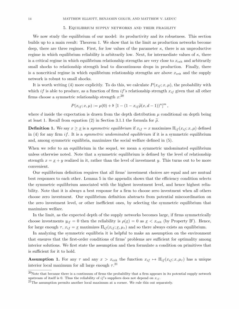
It is worth writing (4) more explicitly. To do this, we calculate P (xif ;x, µ), the probability with
which if is able to produce, as a function of firm if ’s relationship strength xif given that all other
firms choose a symmetric relationship strength x:20
P (xif ;x, µ) := µ(0) + E [1− (1− xif ρ(x, d− 1))n]m ,
where d inside the expectation is drawn from the depth distribution µ conditional on depth being
at least 1. Recall from equation (2) in Section 3.1.1 the formula for ρ.
Definition 1. We say x ≥ x is a symmetric equilibrium if xif = x maximizes Πif (xif ;x, µ) defined
in (4) for any firm if . It is a symmetric undominated equilibrium if it is a symmetric equilibrium
and, among symmetric equilibria, maximizes the social welfare defined in (5).
When we refer to an equilibrium in the sequel, we mean a symmetric undominated equilibrium
unless otherwise noted. Note that a symmetric equilibrium is defined by the level of relationship
strength x = x+ y realized in it, rather than the level of investment y. This turns out to be more
convenient.
Our equilibrium definition requires that all firms’ investment choices are equal and are mutual
best responses to each other. Lemma 5 in the appendix shows that the efficiency condition selects
the symmetric equilibrium associated with the highest investment level, and hence highest relia-
bility. Note that it is always a best response for a firm to choose zero investment when all others
choose zero investment. Our equilibrium definition abstracts from potential miscoordination on
the zero investment level, or other inefficient ones, by selecting the symmetric equilibrium that
maximizes welfare.
In the limit, as the expected depth of the supply networks becomes large, if firms symmetrically
choose investments yif = 0 then the reliability is ρ(x) = 0 as x < xcrit (by Property B′). Hence,
for large enough τ , xif = x maximizes Πif (xif ;x, µτ ) and so there always exists an equilibrium.
In analyzing the symmetric equilibria it is helpful to make an assumption on the environment
that ensures that the first-order conditions of firms’ problems are sufficient for optimality among
interior solutions. We first state the assumption and then formulate a condition on primitives that
is sufficient for it to hold.
Assumption 1. For any τ and any x > xcrit the function xif 7→ Πif (xif ;x, µτ ) has a unique
interior local maximum for all large enough τ .21
20Note that because there is a continuum of firms the probability that a firm appears in its potential supply networkupstream of itself is 0. Thus the reliability of if ’s suppliers does not depend on xif .21The assumption permits another local maximum at a corner. We rule this out separately.
15
Assumption 1 will be maintained in the sequel, along with Properties A, B′, and C. The following
lemma shows that we may always set x so that Assumption 1 is satisfied.
Lemma 1. For any m ≥ 2, and any n ≥ 2, there is a number22 x, depending only on m and n, such
that, for large enough τ we have: (i) x < xcrit; and (ii) if x ≥ x, then Assumption 1 is satisfied.
To see why this lemma implies that Assumption 1 is satisfied for a suitable choice of x, consider
any environment where x ∈ [x, xcrit). Part (i) of the lemma guarantees that the interval [x, xcrit) is
nonempty, and part (ii) guarantees that Assumption 1 is satisfied for values of x in this range.23 In
other words, the lemma guarantees that there is an interval of possible baseline levels of robustness
which are short of the critical level (so that fragility is not ruled out a priori) but high enough to
ensure that the firms’ maximization problem is amenable to a first-order approach.
We now characterize the equilibrium behavior.
Theorem 1. Fix any n ≥ 2, m ≥ 3, and ε > 0.24 There are thresholds κ(n,m) < κ(n,m) and
a threshold τ , so that for all τ ≥ τ there is a unique symmetric undominated equilibrium, with a
relationship strength denoted by x∗τ (κ), satisfying the following properties:
(i) If κ < κ, there is no investment: x∗τ (κ) = x.
(ii) For κ ∈ [κ, κ], the equilibrium relationship strength satisfies x∗τ (κ) ∈ [xcrit− ε, xcrit + ε]. We
call such equilibria critical.
(iii) For κ > κ, the equilibrium relationship strength satisfies x∗τ (κ) > xcrit. We call such
equilibria non-critical.
Moreover, for τ ≥ τ , the function x∗τ (κ) is increasing on the domain κ > κ.
If we think of different supply networks as being parameterized by different values of κ in a
compact set, Theorem 1 implies that in the limit as τ gets large, there will be a positive fraction of
supply networks in which firms will choose relationship strengths converging to xcrit in equilibrium.
This contrasts with the social planner’s solution, which never selects relationship strengths near
xcrit. It also means that a positive fraction of supply networks end up perched on the precipice,
vulnerable to small unanticipated systemic shocks. This vulnerability extends to anticipated shocks,
as discussed in Section 6.2.2.
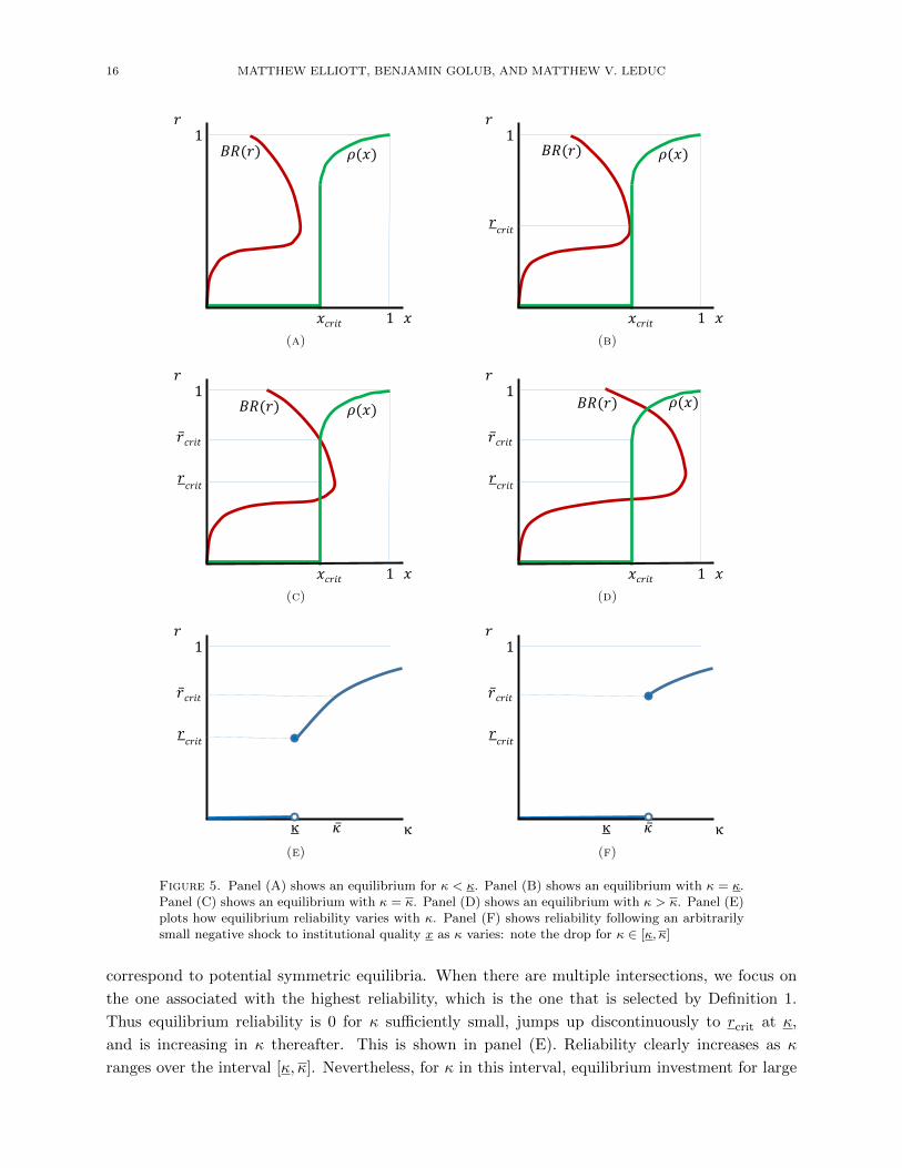
Figure 5 helps give some intuition for Theorem 1. In any symmetric equilibrium, the reliability
of each firm must be consistent with the symmetric investment level x chosen by all other firms—we
must be somewhere on the reliability curve we derived in Section 2. The graphs labeled ρ(x) in
panels (A)–(D) of Figure 5 illustrate the shape of the reliability curve for large τ . Further, in any
symmetric equilibrium each firm’s (symmetric) investment choice of x must be a best response
to the reliability of its suppliers. The curves labeled BR(x) in panels (A)–(D) depict the best-
response function; these curves should be thought of as having their independent variable (others’
reliability) on the vertical axis, and the best-response investment on the horizontal axis. The
panels show the best-response curves for increasing values of κ. Intersections of these two curves
22In the proof, we give an explicit description of x in terms of the shape of the function P (xif ;x, µτ ).23While conditions we identify in Lemma 1 are sufficient for satisfying Assumption 1, they are not necessary.24In this result, we restrict attention to the case of m ≥ 3. It is essential for our results that supply networks arecomplex (m ≥ 2), but the case of m = 2 generates some technical difficulties for our proof technique so we considerm ≥ 3. In numerical exercises, our conclusions seem to also hold for m = 2.
16 MATTHEW ELLIOTT, BENJAMIN GOLUB, AND MATTHEW V. LEDUC
𝑟
𝑥
1
1𝑥𝑐𝑟𝑖𝑡
𝐵𝑅(𝑟) 𝜌(𝑥)
(a)
𝑟
𝑥
1
1𝑥𝑐𝑟𝑖𝑡
𝑟𝑐𝑟𝑖𝑡
𝐵𝑅(𝑟) 𝜌(𝑥)
(b)
𝑟
𝑥
1
1
ҧ𝑟𝑐𝑟𝑖𝑡
𝑥𝑐𝑟𝑖𝑡
𝑟𝑐𝑟𝑖𝑡
𝐵𝑅(𝑟) 𝜌(𝑥)
(c)
𝑟
𝑥
1
1𝑥𝑐𝑟𝑖𝑡
𝑟𝑐𝑟𝑖𝑡
ҧ𝑟𝑐𝑟𝑖𝑡
𝐵𝑅(𝑟) 𝜌(𝑥)
(d)
𝑟
κ
1
𝑟𝑐𝑟𝑖𝑡
ҧ𝑟𝑐𝑟𝑖𝑡
κ ҧ𝜅
(e)
𝑟
κ
1
𝑟𝑐𝑟𝑖𝑡
ҧ𝑟𝑐𝑟𝑖𝑡
κ ҧ𝜅
(f)
Figure 5. Panel (A) shows an equilibrium for κ < κ. Panel (B) shows an equilibrium with κ = κ.Panel (C) shows an equilibrium with κ = κ. Panel (D) shows an equilibrium with κ > κ. Panel (E)plots how equilibrium reliability varies with κ. Panel (F) shows reliability following an arbitrarilysmall negative shock to institutional quality x as κ varies: note the drop for κ ∈ [κ, κ]
correspond to potential symmetric equilibria. When there are multiple intersections, we focus on
the one associated with the highest reliability, which is the one that is selected by Definition 1.
Thus equilibrium reliability is 0 for κ sufficiently small, jumps up discontinuously to rcrit at κ,
and is increasing in κ thereafter. This is shown in panel (E). Reliability clearly increases as κ
ranges over the interval [κ, κ]. Nevertheless, for κ in this interval, equilibrium investment for large
17
τ remains arbitrarily close to xcrit, since the equilibrium is on the essentially vertical part of the
reliability curve. In other words, equilibrium investment choices bunch around xcrit for an open
interval of values of κ. For all κ ∈ [κ, κ] a slight shock causing relationship strengths to diminish
from x to x− ε causes relationship strengths to fall below xcrit, and makes equilibrium production
collapse. Panel (F) shows reliability after such a shock for different values of κ. As can be seen by
comparing panels (E) and (F), the shock does not change the values of reliability at κ below κ or
above κ: the curves in (E) and (F) are essentially identical in those ranges. However, for κ ∈ [κ, κ],
reliability drops discontinuously to 0.
We now pause to comment on the techniques used to establish these results. While the intuition
looks straightforward in our sketches, proving Theorem 1 is technically challenging. We have
to get a handle on the shape of the best-response correspondence, and show that the highest
intersection of it with the reliability curve moves as depicted in Figure 5. Investment incentives
(which determine the shape of the best-response curve, and the implications of changing κ) are
complex, and so equilibrium investment is difficult to characterize directly. We do not have an
explicit expression for the best-response curve. It also does not have any global monotonicity
properties that might permit standard comparative statics approaches. Investments in relationship
strength are strategic complements in some regions of the parameter space, and strategic substitutes
in others.25 However, some control on the slopes of the intersecting curves is necessary to analyze
the dependence of the intersection on parameters. A key step in our analysis is showing that if the
highest intersection of best response and reliability curves is at r ≥ rcrit, then the best response
curve must be negatively sloped in r there, and strictly so for an intersection at r > rcrit. We do
so by establishing certain properties of the system of polynomial equations that (asymptotically)
characterizes the intersection. Another cruicial step is to show that there is at most one point of
intersection above rcrit in our diagrams. This permits us to focus on a unique outcome of interest,
and to sign the effects of moving κ unambiguously, which is important for the results on equilibrium
fragility.
At a technical level, there are two parts to many of our proofs. One part focuses on an idealized
“limit supply network,” which, in a suitable sense, has infinite depth and therefore a lot of symmetry
(a firm’s suppliers look exactly like the firm itself). This symmetric network gives rise to expressions
that we can manipulate to establish the key facts mentioned above. There is then a separate task
of transforming these limit results into statements about the supply network with large but finite
depths.
Our next result, Corollary 1, implies that the comparative statics of equilibrium as the baseline
quality of institutions x changes are analogous to those documented with respect to κ in Theorem
1. Here we explicitly include x as an argument in x∗.
Corollary 1. Suppose κ′ > κ. Then, for large enough τ , if x∗τ (κ′, x) > x∗τ (κ, x), there is an x′ > x
such that x∗τ (κ′, x) = x∗τ (κ, x′).
25When a firm’s suppliers are very unreliable, there is little incentive to invest in stronger relationships with them—there is no point in having a working supply relationship when the suppliers cannot produce their goods. On theother hand, when a firm’s suppliers are extremely reliable, a firm can free-ride on this reliability and invest relativelylittle in its relationships, knowing that as long as it has one working relationship for each input it requires, it is verylikely to be able to source that input.
18 MATTHEW ELLIOTT, BENJAMIN GOLUB, AND MATTHEW V. LEDUC
5.1. Fragility. Critical equilibria are important because, as the example in Figure 5 shows, they
create the possibility of fragility: small unanticipated shocks to relationship strengths via a reduc-
tion in x can result in a collapse of production. We formalize this idea by explicitly examining how
the supply network responds to a shock to the baseline quality of institutions x, which for simplicity
is taken to have zero probability. (The analysis is robust to anticipated shocks that happen with
positive probability—see Section 6.2.2.)
Definition 2 (Equilibrium fragility).
• There is equilibrium fragility at κ if for any η, ε > 0, for large enough τ , we have
ρ(x∗τ (κ)− ε, µτ ) < η.
That is, a shock that reduces relationship strengths arbitrarily little (ε) from their equilib-
rium levels leads to a reliability very close to 0 (within η).
• We say there is equilibrium robustness at κ if there is not equilibrium fragility.
Note that the definition of equilibrium fragility makes sense only if x∗τ (κ) > 0 for all large enough
τ , and this implies reliability bounded away from zero before the shock, since otherwise there would
be no incentive for investment. In the definition of fragility, while shocking x, we hold investment
decisions and entry choices fixed. This corresponds to the assumption, discussed in Subsection 5.2
below, that investments in supply relationships and entry decisions are made over a sufficiently
long time frame that firms cannot change the quality of their supply relationships or their entry
decisions in response to a shock.
Proposition 3. Under the conditions of Theorem 1, there is equilibrium fragility at any κ ∈ [κ, κ]
and equilibrium robustness at any κ > κ.
Proposition 3 follows immediately from the definition of equilibrium fragility and our previous
characterization.
5.2. Some comments on interpretation.
5.2.1. Sources of shocks. There are many ways in which the small systemic shock involved in our
notion of fragility might arise in practice. In the introduction, we discussed the example of a small
shock to credit markets making many supply relationships slightly more likely to fail, if they happen
to require financing to deal with a disruption. Another example comes from considering new trade
regulations: if there is uncertainty about which relationships will be affected by new compliance
issues, each supply relationship will be ex ante more prone to disruption. For a third example,
consider an increasing backlog in commercial courts—a circumstance that makes contracts more
costly to enforce. This again decreases the probability that contracts function in some states of the
world—an uncertainty that can affect many players in the supply chain. A final example comes from
supply chain stresses due to macroeconomic shocks. Technological factors, such as social distancing
measures imposed during a pandemic, can cause stochastic delays and disruptions throughout the
dependency links in a supply network. Congestion provides another type of stress. For example,
a demand shock to some goods can require ports and transportation hubs to accommodate more
traffic, causing queues. These queues delay shipments of goods in many supply networks, even
those not affected by the demand shocks that caused the queues (McLain et al., 2021).
19
5.2.2. Time scales. In interpreting our model, a crucial issue is the time scales on which the con-
tagion occurs, and on which decisions are made. We define the short run to be period of time over
which firms are not able to adjust their relationship strengths. It is this time scale on which the
shock we study has its most direct implications in terms of freezing supply chains. Evidence from
Barrot and Sauvagnat (2016) suggests that in practice this time scale is on the order of magnitude
of several quarters. In contrast, the medium run as a period of time over which adjustments in
relationship strength are possible.26 Thus, following a shock to relationship strengths, in the short
run a collapse in production will occur when the supply network is in the fragile regime—that is,
holding investments in relationship strengths at their old values. In the medium run, it is possible
that firms can choose investment levels that allow the supply network to resume being productive.
Our equilibrium selection here is optimistic: it focuses on the outcome where, in recovering from
the shock, firms coordinate on the most productive investment equilibrium, and thus limit the
losses. Alternatively, once production has become disrupted, it could be that firms stop investing
altogether. If such coordination problems occur, disruptions can be longer-lasting and consistent
with long-lasting productivity damage following a shock.
6. Discussion of the model
This section discusses our modeling choices. First, in Section 6.1 we highlight which features of
our environment are essential, and motivate them. Beyond the key assumptions, we make a variety
of assumptions for tractability or simplicity. In Section 6.2, we discuss the robustness of our model
to various relaxations of these non-essential assumptions.
6.1. Essential features. The three essential features that we highlight are that supply rela-
tionships are specific (firm-to-firm) and subject to disruption; that firms endogenously invest to
strengthen their relationships; and that production is complex in that it relies on multiple essential
inputs at each of a sufficiently large number of layers.
Specific sourcing relationships that are subject to idiosyncratic disruptions are a crucial feature
of our model. Supplier relationships have been found to play important roles in many settings—for
relationship lending between banks and firms see Petersen and Rajan (1994, 1995); for traders in
Madagascar see Fafchamps and Minten (1999); for the New York apparel market see Uzzi (1997);
for food supply chains see Murdoch, Marsden, and Banks (2000); for the diamond industry see
Bernstein (1992); for Japanese electronics manufacturers see Nishiguchi (1994)—and so on. Indeed,
even in fish markets, a setting where we might expect relationships to play a minor role, they seem
to be important (Kirman and Vriend, 2000; Graddy, 2006). The importance of specific sourcing
relationships in supply networks is also a major concern of the management literature on supply
chains (Datta, 2017). Barrot and Sauvagnat (2016) find that firms have difficulty switching suppliers
even when they need to do so. These literatures examine many reasons behind firms’ reliance on a
small number of suppliers to source a given type of input. For example, technological compatibility
and geography can limit the pool of potential suppliers; hold-up problems can make trust important;
and frequent repeated interactions can help firms to avoid misunderstandings.
26Other technological dimensions, such as the complexity m of production, might change on a longer time scale still;see Section 8.4.
20 MATTHEW ELLIOTT, BENJAMIN GOLUB, AND MATTHEW V. LEDUC
The specific relationships that firms maintain for sourcing facilitate the contagion of disruption.
Indeed, cascading disruptions (see, for example, Carvalho et al. (2020)) are evidence of firms’ re-
liance on failure-prone sources of supply that cannot be quickly replaced. Interesting qualitative
descriptions of cascades of disruption due to idiosyncratic shocks can be found in the business litera-
ture. A fire at a Philips Semiconductor plant in March 2000 halted production, preventing Ericsson
from sourcing critical inputs, causing its production to also stop (The Economist , 2006). Ericsson
is estimated to have lost hundreds of millions of dollars in sales as a result, and it subsequently
exited the mobile phone business (Norrman and Jansson, 2004). In another example, two strikes
at General Motors parts plants in 1998 led 100 other parts plants, and then 26 assembly plants,
to shut down, reducing GM’s earnings by $2.83 billion (Snyder et al., 2016). Though these partic-
ular examples are particularly well-documented, disruptions are a more frequent occurrence than
might be expected. In a survey of studies on this subject in operations and management, Snyder
et al. (2016) write, “It is tempting to think of supply chain disruptions as rare events. However,
although a given type of disruption (earthquake, fire, strike) may occur very infrequently, the large
number of possible disruption causes, coupled with the vast scale of modern supply chains, makes
the likelihood that some disruption will strike a given supply chain in a given year quite high.” An
industry study recorded 1,069 supply chain disruption events globally during a six-month period
in 2018 (Supply Chain Quarterly, 2018).
Given the frequency of disruptions and the impact these can have on firms’ profitability,27 it is
natural that firms take actions to mitigate them. In practice, these investments are often “soft”
in nature. A literature in sociology helps document them—a prominent contribution being Uzzi
(1997), who offers a detailed account of the systematic efforts and investments made by New York
garment manufacturers and their suppliers to maintain good relations. These investments include
practices such as building a better understanding of a supplier’s or customer’s capabilities by visiting
their facilities, querying odd instructions to help catch mistakes, building social relationships that
span the organizations, and reciprocal gift-giving. Such investments are hard to observe and even
harder to verify. This makes them hard to contract on and fits the way we model investments—as
a decentralized game of private investment in one’s local relationships.28
It is crucial for our theoretical results that production is complex. One aspect of complexity is in
the horizontal dimension of our network diagrams: firms need multiple inputs via specific sourcing
relationships. Barrot and Sauvagnat (2016) provide evidence that supports this assumption. They
show that if a supplier is hit by a natural disaster it severely disrupts the production of their
customers and also negatively impacts their customers’ other suppliers. If production were not
complex in this way, then these other suppliers would be providing substitute inputs and hence
would benefit from the disruption to a competitor rather than being adversely affected. Similarly,
this suggests that inventories are not held at high enough levels to avoid disruption, though they
27Hendricks and Singhal (2003, 2005a,b) examine hundreds of supply chain problems reported in the business press.Even minor disruptions are associated with significant and long-lasting declines in sales growth and stock returns.28The key feature here is the modeling of investment as a non-cooperative game. Even if firms were allowed to investin others’ relationships they would typically not want to in equilibrium. Following the logic of Bergstrom, Blume,and Varian (1986) each firm will be willing to invest in each relationship (between any two firms) up to the point thatthe marginal return of the investment equals the marginal benefits. However, the marginal benefits are heterogeneousand it will typically only be possible for this condition to be satisfied by the firm that has the highest marginal benefitof investing.
21
may help delay it. Another aspect of complexity is that production takes place in multiple layers—
i.e., is sufficiently deep. As we show in Section SA4 of the Supplementary Appendix, even without
taking any limits, realistic degrees of complexity either in the horizontal or vertical dimension
generate patterns that have the key qualitative features driving our main results.
An example of a firm with a relatively complex supply chain is Toyota. After the Great East
Japan Earthquake Toyota suffered considerable disruption to its supply network due, in part, to
the impact on firms several layers upstream of it. Following this, Toyota made an effort to map out
its supply network so it could better anticipate and respond to such problems. It has been reported
that despite remaining incomplete this mapping got as far as the tenth level and identified 400,000
items that Toyota sources directly or indirectly (McLain, 2021).
One final observation is that our model can be reinterpreted as describing processes or inputs,
rather than firms, as long as the key conditions outlined in this section hold. From this perspective,
the phenomena we discuss may happen within a firm or other organization. Increasing the strength
of relationships would then correspond to increasing various forms of redundancy or robustness
in sourcing. When agency frictions are significant and decisions about robustness are made in a
decentralized way, our model of endogenous investments would also be relevant.
6.1.1. Contrasts with models without the essential features. In this subsection, we briefly consider
two alternative models, which we consider useful benchmarks, to highlight the necessity of key
features discussed in the previous section.
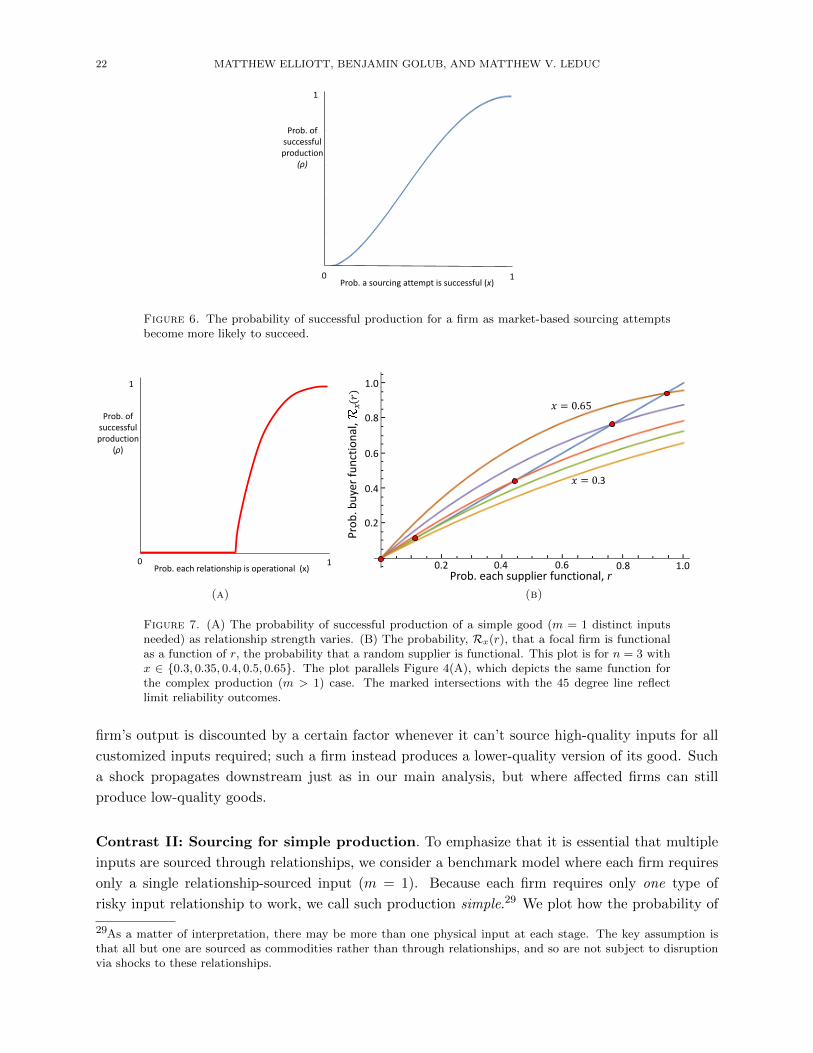
Contrast I: Sourcing through spot markets. In this benchmark, each firm sources all its
inputs through spot markets, rather than requiring pre-established relationships. The market is
populated by those potential suppliers that are able to successfully produce the required input. To
keep the technology of sourcing comparable, we posit that, after a buyer places an order in this
spot market, there is still a chance that sourcing fails. (A shipment might be lost or defective, or a
misunderstanding could lead the wrong part to be supplied.) In other words, we now assume each
firm extends relationships only to functional suppliers (as opposed to suppliers whose functionality is
random, in our main model), but we still keep the randomness in whether the sourcing relationships
work.
We now work out which firms can produce, focusing on the example where each firm requires two
inputs (m = 2). Each firm if multisources by contracting with two potential suppliers of each input
(n = 2)—selected from the functional ones. Let the probability a given attempt at sourcing an
input succeeds be x, independently. The probability that both potential suppliers of a given input
type fail to provide the required input is (1 − x)2, and the probability that at least one succeeds
is 1 − (1 − x)2. As the firm needs access to all its required inputs to be able to produce, and it
requires two different input types, the probability the firm is able to produce is (1 − (1 − x)2)2.
In Figure 6 we plot how the probability that a given firm is able to produce varies with the
probability its individual sourcing attempts are successful. This probability increases smoothly as
x increases. This benchmark thus shows that perfect spot markets remove the discontinuities in
our main analysis.
On the other hand, the fragility of complex production remains a concern even in the presence
of imperfect substitutes for specifically sourced inputs. More precisely, suppose the quality of a
22 MATTHEW ELLIOTT, BENJAMIN GOLUB, AND MATTHEW V. LEDUC
Prob. of successful production
(ρ)
1
10Prob. a sourcing attempt is successful (x)
Figure 6. The probability of successful production for a firm as market-based sourcing attemptsbecome more likely to succeed.
Prob. each relationship is operational (x)10
Prob. of successful production
(ρ)
1
(a)
Pro
b. b
uye
r fu
nct
ion
al,
0.2
0.4
0.6
0.8
1.0
Prob. each supplier functional, r0.2 0.4 0.6 0.8 1.0
𝑥 = 0.3
𝑥 = 0.65(𝑟)
𝑥
(b)
Figure 7. (A) The probability of successful production of a simple good (m = 1 distinct inputsneeded) as relationship strength varies. (B) The probability, Rx(r), that a focal firm is functionalas a function of r, the probability that a random supplier is functional. This plot is for n = 3 withx ∈ {0.3, 0.35, 0.4, 0.5, 0.65}. The plot parallels Figure 4(A), which depicts the same function forthe complex production (m > 1) case. The marked intersections with the 45 degree line reflectlimit reliability outcomes.
firm’s output is discounted by a certain factor whenever it can’t source high-quality inputs for all
customized inputs required; such a firm instead produces a lower-quality version of its good. Such
a shock propagates downstream just as in our main analysis, but where affected firms can still
produce low-quality goods.
Contrast II: Sourcing for simple production. To emphasize that it is essential that multiple
inputs are sourced through relationships, we consider a benchmark model where each firm requires
only a single relationship-sourced input (m = 1). Because each firm requires only one type of
risky input relationship to work, we call such production simple.29 We plot how the probability of
29As a matter of interpretation, there may be more than one physical input at each stage. The key assumption isthat all but one are sourced as commodities rather than through relationships, and so are not subject to disruptionvia shocks to these relationships.
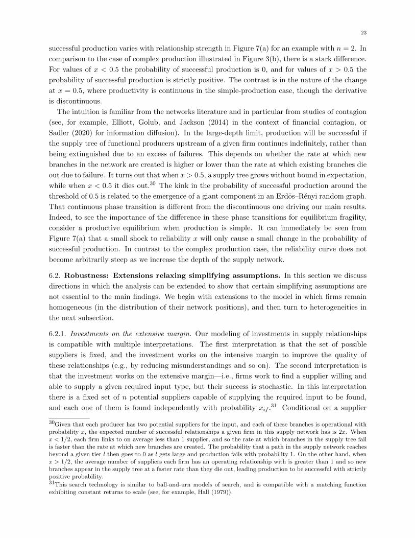
23
successful production varies with relationship strength in Figure 7(a) for an example with n = 2. In
comparison to the case of complex production illustrated in Figure 3(b), there is a stark difference.
For values of x < 0.5 the probability of successful production is 0, and for values of x > 0.5 the
probability of successful production is strictly positive. The contrast is in the nature of the change
at x = 0.5, where productivity is continuous in the simple-production case, though the derivative
is discontinuous.
The intuition is familiar from the networks literature and in particular from studies of contagion
(see, for example, Elliott, Golub, and Jackson (2014) in the context of financial contagion, or
Sadler (2020) for information diffusion). In the large-depth limit, production will be successful if
the supply tree of functional producers upstream of a given firm continues indefinitely, rather than
being extinguished due to an excess of failures. This depends on whether the rate at which new
branches in the network are created is higher or lower than the rate at which existing branches die
out due to failure. It turns out that when x > 0.5, a supply tree grows without bound in expectation,
while when x < 0.5 it dies out.30 The kink in the probability of successful production around the
threshold of 0.5 is related to the emergence of a giant component in an Erdos–Renyi random graph.
That continuous phase transition is different from the discontinuous one driving our main results.
Indeed, to see the importance of the difference in these phase transitions for equilibrium fragility,
consider a productive equilibrium when production is simple. It can immediately be seen from
Figure 7(a) that a small shock to reliability x will only cause a small change in the probability of
successful production. In contrast to the complex production case, the reliability curve does not
become arbitrarily steep as we increase the depth of the supply network.
6.2. Robustness: Extensions relaxing simplifying assumptions. In this section we discuss
directions in which the analysis can be extended to show that certain simplifying assumptions are
not essential to the main findings. We begin with extensions to the model in which firms remain
homogeneous (in the distribution of their network positions), and then turn to heterogeneities in
the next subsection.
6.2.1. Investments on the extensive margin. Our modeling of investments in supply relationships
is compatible with multiple interpretations. The first interpretation is that the set of possible
suppliers is fixed, and the investment works on the intensive margin to improve the quality of
these relationships (e.g., by reducing misunderstandings and so on). The second interpretation is
that the investment works on the extensive margin—i.e., firms work to find a supplier willing and
able to supply a given required input type, but their success is stochastic. In this interpretation
there is a fixed set of n potential suppliers capable of supplying the required input to be found,
and each one of them is found independently with probability xif .31 Conditional on a supplier
30Given that each producer has two potential suppliers for the input, and each of these branches is operational withprobability x, the expected number of successful relationships a given firm in this supply network has is 2x. Whenx < 1/2, each firm links to on average less than 1 supplier, and so the rate at which branches in the supply tree failis faster than the rate at which new branches are created. The probability that a path in the supply network reachesbeyond a given tier l then goes to 0 as l gets large and production fails with probability 1. On the other hand, whenx > 1/2, the average number of suppliers each firm has an operating relationship with is greater than 1 and so newbranches appear in the supply tree at a faster rate than they die out, leading production to be successful with strictlypositive probability.31This search technology is similar to ball-and-urn models of search, and is compatible with a matching functionexhibiting constant returns to scale (see, for example, Hall (1979)).

24 MATTHEW ELLIOTT, BENJAMIN GOLUB, AND MATTHEW V. LEDUC
being found, the relationship is operational. In Supplementary Appendix SA6 we discuss a richer
extensive-margin interpretation, and also one that permits separate efforts to be directed to the
extensive and intensive margins simultaneously.
6.2.2. Anticipated shocks. We assume that the small shock to x is unanticipated. It is straightfor-
ward to use our analysis to see that this is not essential. Suppose now all firms anticipate that
a shock to x will happen with some probability pshock, and suppose κ is in an open subset of the
critical productivities, so that a collapse would have occurred in the baseline model. When we
write the profit function for firms in the extended model, there will now be an expectation over the
shock’s arrival, and this will change profits and the best-response correspondence. However, for a
small enough probability of the shock, this change will be small, and the best-response curve in a
plot such as Figure 5(c) will move only slightly. Thus the equilibrium will still be on the precipice
if it was before. Indeed, for κ not too close to the boundary of the critical productivities, the
probability of the shock can be quite substantial without changing the main prediction. The key
intuition is that because of externalities, while all firms may prefer a commitment to invest more
to avoid being on the precipice (and avoid disruptions due to the shock), the free-riding problem
can be too severe to achieve this. Indeed, note that in Figure 5, even fairly large shifts in the best-
response curve can leave the equilibrium on the precipice, implying that these free-riding effects
are considerable.
6.2.3. Shocks to firms. The fundamental source of shocks in our model is at the level of links in the
supply network. One could also consider shocks directly hitting firms—i.e., shocks to nodes in our
supply network rather than links. The key conclusions regarding precipices are robust to adding
this source of shocks, or even making node-level shocks the main source of disruptions.32 We focus
on shocks to relationships for simplicity, but the mathematical forces we identify also operate in
alternative models of disruption.
6.2.4. Endogenous entry. Our model takes the varieties in the market as given, and does not include
entry decisions by firms. This is done to keep the model simple. However, the key insights carry
over in a model with entry.
Consider an extended model where there is an entry stage preceding all others. At this stage, a
firm (i, f) pays a sunk entry cost Φ(f), where Φ is a strictly increasing function. Then the measure
of varieties in each product is set equal to the measure of entering firms (i.e., each entering firm
produces one variety), and the “investment game” where firms choose their relationship strengths
proceeds as we described earlier. A (nontrivial) symmetric equilibrium is now one where f > 0
firms enter in each product and the expected post-entry profits of the marginal firm are equal to
its entry cost.
The main observation is that this model also features an open set of productivity parameters
κ where equilibrium production is on the precipice. The basic logic is as follows. When the
supply network is reliable and gross profits after entry are high, firms want to enter. As they
enter, competition drives down gross profits and makes it less appealing to pay costs to make
relationships strong. Recalling Figure 5, the key to the argument is that increasing entry moves
the best-response curve leftward for a given κ. So, in equilibrium, relationships get weaker as more
32This variant of the model is worked out in Elliott and Golub (2021).

25
entry occurs. The question is where this dynamic stops. The precipice is a natural stopping point.
Once the investment level is xcrit, reliability can adjust down until further entry is deterred, while
investment remains the same. By reasoning parallel to that of our main results, this state is reached
for an open set of model parameters.
6.3. Robustness to heterogeneity. We have so far assumed for tractability that all firms have
identical network positions ex ante. One might suspect that the regularity of the network structure,
or some other kind of homogeneity, plays an important role in generating the sharp transition in the
probability of successful production. In contrast with the key roles played by complexity, specific
sourcing, and depth, homogeneities across the firms are not important to our main points. To
establish this, we now discuss extensions with two forms of heterogeneity in firm type.
6.3.1. Partial knowledge of depth. We have assumed that firms make investments ex ante of the
realization of their supply network depths, so that when they face their investment decisions, they
have identical decision problems. This implies that they all have identical investment incentives,
a symmetry that simplifies the analysis considerably. However, in practice, firms do have some
information about the depth of their supply networks. We now introduce this into the model and
give conditions under which our main findings extend.
We refer to the model analyzed in Sections 3–5 as the baseline model, and we will define the
model with partial knowledge of depths with reference to it.
The firms are now partitioned into two types: low-depth firms, with depth less than or equal
to dl ≥ 0, constitute a proportion µl < 1 of the population, and high-depth firms, with depth
greater than dl, constitute the remainder. (We discuss the case of more than two types below.)
Firms’ information about depth consists of knowing which type they are. We use the subscript l
for low-depth firms and h for the high-depth firms.
Each type of firm has gross profits from production equal to gt(rt), where rt is the aggregate
reliability of that type of firm (t = l for low-depth firms, and t = h for high-depth ones). This
amounts to assuming that each type of firm sells into a separate market, and its gross profits are
dependent on competition in that market through rt. Similarly, each type of firm has a cost function1κtct. The model is otherwise the same, with the functions gt and ct satisfying the assumptions
made on g and c, respectively, in the homogeneous model.
We now extend the definition of equilibrium to allow low-depth and high-depth firms to behave
differently; equilibrium again refers to a symmetric Nash equilibrium that is not Pareto-dominated
by any other symmetric equilibrium, but where symmetric now means that strategy depends only
on type. We let the vector x∗τ (κl, κh) denote relationship strengths for the low-depth and high-depth
firms in such an equilibrium.
Our focus will be on the high-depth firms. We thus define an equilibrium to be fragile if, for large
enough typical depth, a very small shock causes the high-depth firms to have very low reliability.
Definition 3 (Equilibrium fragility with partial knowledge of depth). There is equilibrium fragility
at κ = (κl, κh) if for any η, ε > 0, for large enough τ , we have
ρh(x∗τ (κ)− ε, µτ ) < η.
That is, a shock that reduces relationship strengths arbitrarily little (ε) from their equilibrium
levels leads to a reliability very close to 0 (within η) for the high-depth firms.
26 MATTHEW ELLIOTT, BENJAMIN GOLUB, AND MATTHEW V. LEDUC
Proposition 4. Suppose there is equilibrium fragility at κ in the baseline model under gross
profit function g. Then in a partial knowledge of depth model with gh = g, the following holds: If
x∗h(κ) > 0 for all sufficiently large τ (i.e. there is positive investment), then there is also equilibrium
fragility.
To gain some intuition for the result, note that in a (symmetric undominated) equilibrium,
the high-depth firms take the reliability of the low-depth firms as given. In particular, all low-
depth firms that the high-depth firms source from are at depth exactly dl and hence have the
same reliability. For κh = κ the high-depth firms are then in an equivalent position to firms in
our baseline model, except that the firms at depth dl play the role of the depth-zero firms in
the baseline model. In that model, the depth zero firms have reliability 1. In the partial depth
knowledge model, the depth dl firms have some reliability r ≤ 1. Nevertheless, as long as r ≥ rcrit
this difference does not matter for τ sufficiently high. The reason for this is that in both cases,
given the same investment decisions for the high-depth firms, limit reliability will be the same as
in the baseline model for those firms by the argument in Subsection 3.1.1. Our assumption that
there is equilibrium fragility at κ in the baseline model implies that, in that model, the limit of
equilibrium investment is xcrit. The proof shows that there will also be limit investment xcrit for the
high-depth firms in the symmetric undominated equilibrium of the extended model (as τ →∞).
This leaves the case when the reliability of the depth d` firms is r < rcrit. We just need to show
that in this case limit reliability is either 0 or rcrit. Hence it is sufficient to rule out limit equilibrium
investment x > xcrit. Such investment cannot be supported in equilibrium for the same reasons
that it could not be supported in the corresponding baseline model.
It is important for interpreting Proposition 4 that we know the high-depth firms are sometimes
in the first positive-investment case, since positive investment is required for equilibrium fragility
to make sense. To show that the positive-investment assumption is not vacuous, note that we can
always set κl sufficiently high to induce equilibrium investments for the low-depth firms above xcrit,
which is sufficient for ensuring the reliability of depth dl firms is above rcrit.
When there is equilibrium fragility, it is only the high-depth firms that are affected. Moreover,
the low-depth firms operate independently of the high-depth firms, and so even if production is
disrupted for all the high-depth firms, the low-depth firms can still produce. This readily extends
to a finer partitioning of firms by their depth. In this case, those firms in all but the highest depth
group have bounded depth and behave like the low-depth firms; the highest-depth group would
behave like the high-depth firms. Extending the model to include partial knowledge of depth, as
we have done in this section, changes the quantitative implications of the model—fewer firms in
a supply chain will be on the precipice—but not the qualitative implications insofar as a positive
mass of the firms will be on the precipice. The discussion in Section 6.1 suggests that a considerable
number of high-value products would be included in this set.
It is worth noting that, for simplicity, we have firms depend on others upstream of themselves
(their suppliers, their suppliers’ suppliers, and so on) but not downstream.33 If the profits of
low-depth firms were instead derived from selling to high-depth firms, then the inability of the
high-depth firms to produce would, via reduced demand for the low-depth firms’ products, affect
33In our microfoundations (Appendix C), the upstream but not downstream dependence is modeled by letting allfirms sell to final consumers, and letting all profits be derived from such sales.
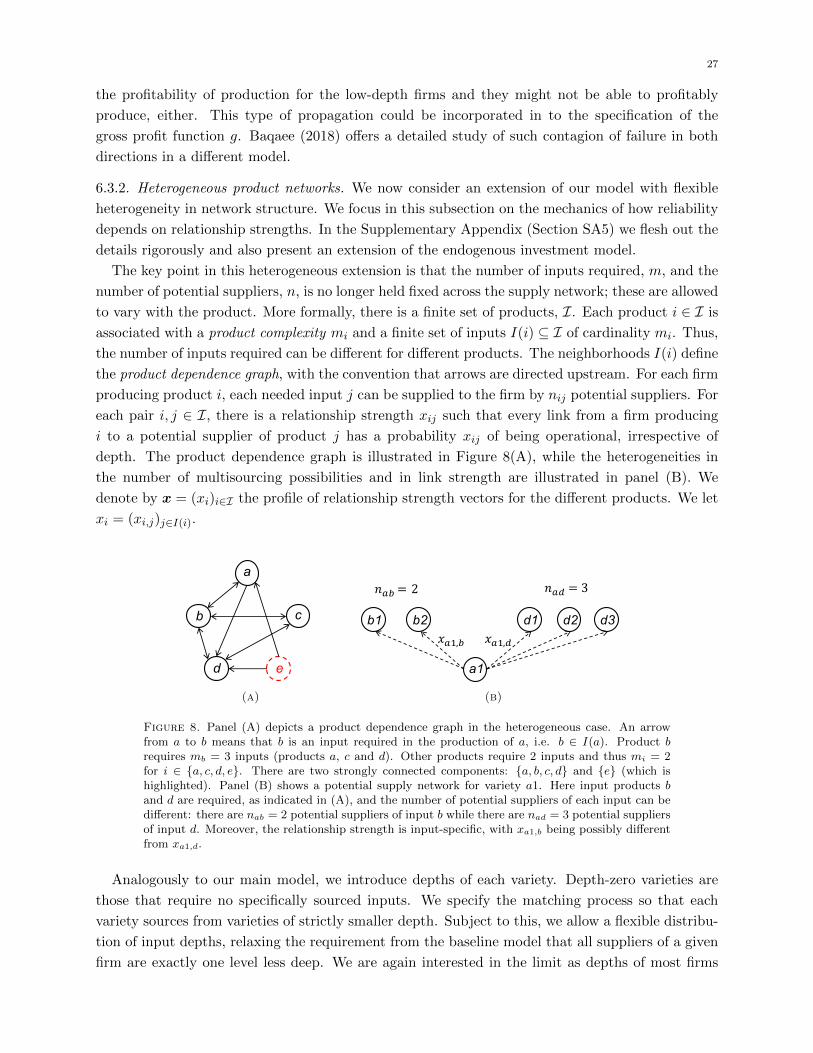
27
the profitability of production for the low-depth firms and they might not be able to profitably
produce, either. This type of propagation could be incorporated in to the specification of the
gross profit function g. Baqaee (2018) offers a detailed study of such contagion of failure in both
directions in a different model.
6.3.2. Heterogeneous product networks. We now consider an extension of our model with flexible
heterogeneity in network structure. We focus in this subsection on the mechanics of how reliability
depends on relationship strengths. In the Supplementary Appendix (Section SA5) we flesh out the
details rigorously and also present an extension of the endogenous investment model.
The key point in this heterogeneous extension is that the number of inputs required, m, and the
number of potential suppliers, n, is no longer held fixed across the supply network; these are allowed
to vary with the product. More formally, there is a finite set of products, I. Each product i ∈ I is
associated with a product complexity mi and a finite set of inputs I(i) ⊆ I of cardinality mi. Thus,
the number of inputs required can be different for different products. The neighborhoods I(i) define
the product dependence graph, with the convention that arrows are directed upstream. For each firm
producing product i, each needed input j can be supplied to the firm by nij potential suppliers. For
each pair i, j ∈ I, there is a relationship strength xij such that every link from a firm producing
i to a potential supplier of product j has a probability xij of being operational, irrespective of
depth. The product dependence graph is illustrated in Figure 8(A), while the heterogeneities in
the number of multisourcing possibilities and in link strength are illustrated in panel (B). We
denote by x = (xi)i∈I the profile of relationship strength vectors for the different products. We let
xi = (xi,j)j∈I(i).
b
a
c
d e
(a)
b1 b2 d1 d2 d3
a1
𝑛!"= 2 𝑛!# = 3
𝑥!$," 𝑥!$,#
(b)
Figure 8. Panel (A) depicts a product dependence graph in the heterogeneous case. An arrowfrom a to b means that b is an input required in the production of a, i.e. b ∈ I(a). Product brequires mb = 3 inputs (products a, c and d). Other products require 2 inputs and thus mi = 2for i ∈ {a, c, d, e}. There are two strongly connected components: {a, b, c, d} and {e} (which ishighlighted). Panel (B) shows a potential supply network for variety a1. Here input products band d are required, as indicated in (A), and the number of potential suppliers of each input can bedifferent: there are nab = 2 potential suppliers of input b while there are nad = 3 potential suppliersof input d. Moreover, the relationship strength is input-specific, with xa1,b being possibly differentfrom xa1,d.
Analogously to our main model, we introduce depths of each variety. Depth-zero varieties are
those that require no specifically sourced inputs. We specify the matching process so that each
variety sources from varieties of strictly smaller depth. Subject to this, we allow a flexible distribu-
tion of input depths, relaxing the requirement from the baseline model that all suppliers of a given
firm are exactly one level less deep. We are again interested in the limit as depths of most firms
28 MATTHEW ELLIOTT, BENJAMIN GOLUB, AND MATTHEW V. LEDUC
become arbitrarily large. In Appendix SA5 we present the details of this setup and characterize
this limit, paralleling Section 3.1 in the homogeneous case. This analysis yields a limit reliability
correspondence ρ mapping x to a profile (ri)i∈I of reliabilities. The correspondence has the prop-
erty that, for any x, if depths are sufficiently large, the reliabilities are arbitrarily close to those
given by ρ.
Our first main result is that the sharp transition in the production function persists in the
heterogeneous model. There are values of the vector x where arbitrarily small shocks to relationship
strengths result in large drops in reliability. The following definition is helpful for making this point:
Definition 4 (Critical product). The product i is critical at x if the product has positive reliability
ρi(x) > 0 at strengths x, but has reliability ρi(x′) = 0 at any profile x′ of strengths that is
elementwise strictly lower than x.
In Section SA5.1 we generalize Proposition 1 by giving conditions guaranteeing that critical products
exist in the heterogeneous model. The key condition is, as before, that production requires mi ≥ 2
distinct inputs at each step.
We next show that supply networks in the presence of heterogeneities feature a weakest link
property (Proposition 5): When one product is critical, all products that rely directly or indirectly
on it are critical as well.34 This result uses the notion of a product dependence graph, whose nodes
are a set I of products, and products have directed links to the input products they require (see
Figure 8(A) for an illustration).
Proposition 5 (Weakest link property).
(i) Suppose product i is critical. Then any product that has a directed path to i in the product
dependence graph is critical.
(ii) Let ISC ⊂ I be a set of products that are part of a strongly connected component of the
product dependence graph. Then any equilibrium with positive effort is such that either all
producers of products i ∈ ISC are critical or no producers of products i ∈ ISC are critical.
Proposition 5 asserts that supply networks suffer from a weakest link phenomenon. First, in Part
(i), we see that if a product is critical, then any small systemic shock (which causes it to fail, by
definition of criticality) causes the failure of all other products that use it as an input, directly or
indirectly. For example, in Figure 8(A), we see that if product b is critical, then a small systemic
shock to relationship strengths causes its production to fail and will also cause products a, c, d and
e to fail. Products a, c, d fail because they use b directly as an input. Product e fails because it
indirectly uses product b as an input (through a and d).
Second, in Part (ii), we begin by recalling that a strongly connected component of the product
dependence graph is a set of nodes (i.e. products) where each node can be reached from any other
node in that set by following some directed path of dependencies. For example, in the product
dependence graph of Figure 8(A), the nodes represented by full black circles (a, b, c and d) form
such a strongly connected component. Node e is not part of this component since it cannot be
reached from the other nodes by following the direction of the arrows. A strongly connected
component of products is a set of products such that each product is used as input (directly or
34Thus, as in Bimpikis, Ehsani, and Ilkılıc (2019b) the social planner has different gains from intervening in differentparts of the network (see their Proposition 8).

29
indirectly) by every other product of that set. This is precisely the intuition behind the fact that
such a component is only as strong as its weakest link. Indeed, if one product is critical, then all
products in that component are also critical at the same time.
In Section SA5.3 of the Supplementary Appendix, we provide proofs supporting this section and
illustrate both the discontinuities and the weakest link property with numerical examples. We also
extend our endogenous investment model and show that the configurations we have described are
consistent with strategic investment in relationship strength.
7. Related literature
We have already discussed many papers that are relevant for motivating our assumptions or
interpreting our results in Section 6. In this section we review several high-level connections to
related literatures not covered by our previous discussions.
There has been considerable recent interest in markets with non-anonymous trade mediated by
relationships.35 The work most closely related to ours in this area also studies network formation
in the presence of shocks. This includes work in the context of production (e.g., Fafchamps (2002),
Levine (2012), Brummitt, Huremovic, Pin, Bonds, and Vega-Redondo (2017), Bimpikis, Candogan,
and Ehsani (2019a), Yang, Scoglio, and Gruenbacher (2019), Amelkin and Vohra (2019)), work on
financial networks (e.g., Cabrales, Gottardi, and Vega-Redondo (2017), Elliott, Hazell, and Georg
(2018), Erol (2018), Erol and Vohra (2018), Jackson and Pernoud (2019)), and other contexts
(e.g., Blume, Easley, Kleinberg, Kleinberg, and Tardos (2011) Jackson, Rodriguez-Barraquer, and
Tan (2012), Talamas and Vohra (2020)). More broadly, the aggregate implications of relying on
relationships to transact have been studied across a variety of settings. For work on thin financial
markets see, for example, Rostek and Weretka (2015), for buyer-seller networks see, e.g., Kranton
and Minehart (2001), and for intermediation see, e.g., Gale and Kariv (2009). Our work focuses
on network formation for production and emphasizes the distinctive network formation concerns
that arise due to strong complementarities. At a methodological level, we offer an approach that
may be useful more broadly. Agents make a continuous choice that determines the probability of
their relationships operating successfully. The links that form may, however, fail in a “discrete”
(i.e., non-marginal) way. The first feature makes the model tractable, while the second one yields
discontinuities in the aggregate production function and distinguishes the predictions from models
where the aggregate production function is differentiable. It might be thought that aggregating over
many supply chains, these discontinuities would be smoothed out at the level of the macroeconomy;
we show they are not.
There is a vibrant literature in macroeconomics on production networks. This literature dates
back to investigations of the input-output structure of economies and the implications of this
(Leontief, 1936). Carvalho and Tahbaz-Salehi (2019) provides a comprehensive survey.
Two recent developments in the literature are particularly relevant to our work: (i) the modeling
of the endogenous determination of the input-output structure; and (ii) a firm-level approach
as opposed to considering inter-industry linkages at a more aggregated level. Some of the most
relevant work on these issues includes Atalay, Hortacsu, Roberts, and Syverson (2011), Oberfield
(2018), Carvalho and Voigtlander (2014), Acemoglu and Azar (2020), Boehm and Oberfield (2020),
35A literature in sociology emphasizes the importance of business relationships, see for example Granovetter (1973)and Granovetter (1985). For a survey of related work in economics see Goyal (2017).
30 MATTHEW ELLIOTT, BENJAMIN GOLUB, AND MATTHEW V. LEDUC
Tintelnot, Kikkawa, Mogstad, and Dhyne (2018), Liu (2019), Acemoglu and Tahbaz-Salehi (2020),
and Konig, Levchenko, Rogers, and Zilibotti (2019). Baqaee and Farhi (2019) and Baqaee and Farhi
(2020) focus specifically on the implications of nonlinearities, and discuss how nonlinearities in firms’
production functions propagate and aggregate up. Whereas they focus on smooth nonlinearities, we
show that especially extreme nonlinearities—discontinuities—naturally come from complex supply
networks. We have discussed throughout how our explicit modeling of sourcing failures in complex
production at the micro level gives rise to new effects (see Section 6.1.1).
The strong complementarities in production in our model are crucial for creating fragility, and
this aspect of our work builds on a large literature following the seminal work of Kremer (1993).
This literature argues that complementarities can help provide a unified account of many economic
phenomena. These include very large cross-country differences in production technology and ag-
gregate productivity; rapid output increases during periods of industrialization; and the structure
of production networks and international trade flows; see, among many others, Ciccone (2002),
Acemoglu, Antras, and Helpman (2007), Levchenko (2007), Jones (2011) and Levine (2012).36 A
possible concern with this literature is that if firms were allowed to take actions that mitigate
supply risks (for example, by multisourcing), that this would endogenously dampen the crucial
complementarities. Our work helps address this concern. We show that even when firms can take
actions to mitigate their risk by multisourcing, a very severe form of equilibrium fragility—and
hence production complementarities—arises.
At a technical level, our work is related to a recent applied mathematics literature on so-called
multilayer networks and their phase transitions (Buldyrev, Parshani, Paul, Stanley, and Havlin,
2010). Discontinuities such as the one we study are termed first-order phase transitions in this liter-
ature.37 Buldyrev, Parshani, Paul, Stanley, and Havlin (2010), and subsequent papers in this area
such as Tang, Jing, He, and Stanley (2016) and Yang, Scoglio, and Gruenbacher (2019), study quite
different network processes, typically with exogenous networks. We show that discontinuous phase
transitions arise in canonical models of production networks, once specific sourcing relationships
are taken into account. Importantly, we also endogenize investments affecting the probabilities of
disruption (which are taken to be exogenous in this literature) and elucidate a new economic force
endogenously putting equilibria on a precipice. Dasaratha (2021) studies endogenous investment
in a random network in an information-sharing model without aggregate uncertainty. Predating
the recent literature just discussed, Scheinkman and Woodford (1994) used insights from physics
models on self-organized criticality to provide a “sandpile” model of the macroeconomy in which
idiosyncratic shocks have large aggregate effects.38 The setup and behavior of the model are rather
different from ours: the main point of commonality is in the concern with endogenous fragility.
In our model, investments in supply relationships leave the supply network robust to idiosyncratic
shocks, but very sensitive to arbitrarily small systemic shocks to relationship strength.
36Prior to his literature, Jovanovic (1987) examines how strategic interdependencies or complementarities can produceaggregate volatility in endogenous variables despite only seemingly “diversifiable” idiosyncratic volatility in exogenousvariables.37These can be contrasted with second-order phase transitions such as the emergence of a giant component in acommunication network, which have been more familiar in economics—see Jackson (2008).38Endogenously, inventories reach a state analogous to a sandpile with a critical slope, where any additional shock(grain dropped on the sandpile) has a positive probability of leading to an avalanche.
31
8. Concluding discussions
We conclude by sketching some implications of our analysis. We first note some basic welfare
implications of the model, complementing the descriptive analysis of fragility that has been our focus
so far. We then turn to the implications for policy approaches aimed at improving the robustness of
supply networks. Finally, we briefly suggest some potential applications of the precipice phenomena
in macroeconomic modeling and studies of industrial development.
8.1. Welfare implications. In Section 4.1 we showed that a planner would never choose invest-
ments that result in the supply network being fragile. On the other hand, in Section 5 we found
that decentralized investment choices often result in fragile supply networks. We now show that
there is systemic underinvestment in reliability at fragile equilibria and discuss the structure of
externalities.
There are three externalities present when a firm chooses its reliability. First, there is the non-
appropriability of consumer surplus. Output is higher when more firms function, and this is not
fully internalized in a firm’s reliability choice even with respect to adding its own variety to the
mix, since the firm appropriates only part of the surplus. Second, there are reliability spillovers:
firms don’t internalize their contributions to helping other varieties function. The reliability of a
firm’s intermediate good production increases the reliability, and hence profitability, of those firms
sourcing from it, the firms sourcing from these firms, and so on. Both the non-appopriability of
consumer surplus and the reliability spillover lead to underinvestment in reliability (all else equal).
On the other hand, there is also a business-stealing effect. Producers of a good make fewer sales
when more producers of the same good are functional. This is a force for overinvestment, all else
equal, as firms jockey to capture a larger share of the market.39
Consider a critical equilibrium. We know from Section 4.1 that reliability investments are never
efficient in a fragile equilibrium. The marginal improvement in reliability from a uniform increase in
investments is arbitrarily large—indeed, this is how we concluded that the planner never chooses re-
liability that leads to a fragile supply network. So, in a critical equilibrium, the non-appropriability
of consumer surplus and reliability spillovers together dominate the business-stealing effect, and
there is underinvestment in relationships relative to an efficient benchmark.
In fact, something much stronger than this is true: there is always underinvestment in relation-
ship strengths in a productive equilibrium. This result follows from the proof of Lemma 5 in the
appendix, which underlies our selection of the high-reliability equilibrium as the efficient one.
Corollary 2. Suppose we have a symmetric equilibrium with relationship strengths x ≥ xcrit.
Then40 x < xSP (κ, µ).
This motivates an interest in policies that increase investment, as this both increases welfare and
has the potential to mitigate fragility. We turn to these next.
8.2. Implications for policies supporting investment and robustness. Counteracting un-
derinvestment and removing fragility is not straightforward. Here we discuss several intuitive policy
39Higher investments in reliability increase the probability a firm is able to function and compete, and so can beinterpreted as an investment in (stochastic) entry. In light of this it is unsurprising that the usual non-appropriabilityof consumer surplus and business-stealing effects are present.40Note that xSP (κ, µ) is single-valued for such values of x, so we may treat xSP as a function here, abusing notation.
32 MATTHEW ELLIOTT, BENJAMIN GOLUB, AND MATTHEW V. LEDUC
interventions that have limited effects, and others that have more potential to qualitatively change
the robustness of the system.
As we noted in Section 5.2.2, we view investments as being chosen in the medium run, an ex ante
decision that does condition on shock realizations. Some policies will affect investment decisions on
this timescale. In contrast, a shock causes disruption in the short run, a timescale on which firms
cannot adjust their investment decisions. However, some policies may be able to react to shocks on
this shorter timescale. We will analyze policies in both horizons, beginning with the medium run
investment decision.
8.2.1. Marginal interventions on investment incentives. Suppose investment in link strength is sub-
sidized to reduce the marginal cost of investments, making the cost of a given investment 1 − θtimes its original cost. More precisely, we make the gross profit equal to
Πif = P (xif ;x)︸ ︷︷ ︸prob. functional
g(r)︸︷︷︸gross profitif functional
−(
1− θκ
)c(yif )︸ ︷︷ ︸
cost of effort
.
Suppose the status quo were at a critical equilibrium with reliability r = r (see Figure 5(B) for
an illustration). A subsidy of this form will shift the red best response curve in Figure 5(B) to
the right. At the margin this will increase reliability, but have a very limited effect on equilibrium
investments for high values of τ . Thus the equilibrium will remain fragile. The same argument can
be used for increasing κ. This leads to the counterintutive conclusions that a policy intervention
that works well in terms of increasing reliability in normal times can still fail to remove fragility to
aggregate shocks.
Indeed, a similar analysis applies for many other interventions that shift the best response curve
to the right—including, for example, improvements in institutions that increase x marginally.
8.2.2. Larger interventions to improve investment. While marginal interventions typically fail to
resolve fragility, non-marginal interventions might work, for the reasons apparent in the earlier
discussion (see also Figure 5(B)). They can shift the equilibrium into the non-fragile regime from
the fragile one. The kinds of policies that would work here would be substantial subsidies to
investments in reliability strength or actions that increase profitability in an industry. This could
be done in a variety ways: large tax exemptions might be granted or competition might be limited
by, for example, improved patent protections.
Such interventions have the flavor of “big push” policies advocated for developing counties to
escape poverty traps, but are different in a few ways from the standard analysis (Murphy et al.,
1989).41 The standard theory underlying a “big push” approach is one of multiple equilibria: there
is a low-output equilibrium with traditional production where demand is low and traditional tech-
nologies are more cost-effective, and a high-output equilibrium with industrialized production where
demand is high and industrial technologies are more cost-effective. For an economy to grow out
of the bad equilibrium, it must do so in a balanced way to take advantage of one sector’s growth
fueling other sectors’ demands, beyond external economies of scale that are confined in a given
industry (Rosenstein-Rodan, 1943). A temporary intervention that subsidizes industrial technol-
ogy can facilitate this shift. Crucially, the good equilibrium is sustained by increased production
41See also Okuno-Fujiwara (1988) and Rodrik (1996).
33
under the same institutions. Once a temporary intervention is removed, the technology and other
economic primitives remain unchanged: in particular, there is no long-term government support of
production, and no institutional changes.
In our analysis we select undominated equilibria and so there is no scope for policies to facilitate
coordination on better equilibria. However, without this selection temporary interventions could
shift an economy out of a bad equilibrium and into a good one, just as in “big push” theories.
Nevertheless, in the fragile regime which is our main focus, all of the productive equilibria involve
fragility, and so no temporary policy can remove it. To resolve fragility, permanent intervention
on costs or production technologies is necessary.42 To summarize, the comparison to classic big-
push models is interesting: we also find an important role for non-marginal interventions, but for
different reasons and with different implications for policy.
8.2.3. Targeting interventions. Our analysis offers some tentative suggestions for how interventions
should be targeted to best address fragility. For targeting questions to make sense, there must be
some heterogeneity across the economy. One type of heterogeneity was introduced in the extension
of Section 6.3.1 with partial knowledge of depth. We first consider interventions that will take a
supply network out of the fragile regime in the environment presented there. In any productive
equilibrium, the equilibrium reliability of the low-depth firms does not affect the limit reliability of
the high-depth firms. Hence further improvements in reliability for the low-depth firms will have no
impact on the reliability of high-depth firms as their depth gets large. On the other hand, targeting
the high-depth firms for non-marginal interventions such as those discussed above may be able to
move the supply network out of the fragile regime.
This relates to the issue of reshoring—bringing production that had been outsourced to offshore
suppliers back into a rich country. The rationale for reshoring through the lens of the model is as
follows. Links involving long-distance shipping to different countries are more prone to disruption
and may occur under weaker institutions. Reshoring can therefore be modeled as improving the
strength of relationships among those firms involved, or improving the technology for investing in
those relationships. The analysis in the previous paragraph suggests that if reshoring targets parts
of the supply network that are of low depth (and known to be so by the participating firms), the
impact is likely be relatively limited. Reshoring high-depth, complex, products, on the other hand,
can be quite effective.
Targeting can also be considered in the model of Section 6.3.2 with richer heterogeneity in the
production structure. There we showed that there is generally a “weakest link” phenomenon in
which all firms downstream of an industry that is fragile are also fragile (Proposition 5). Thus,
policymakers should be especially interested in identifying upstream, or central, complex industries
in a critical equilibrium. We would expect the industries at risk to be ones with relatively low
profit margins and relatively few sourcing options per firm. Beyond these guidelines, a diagnostic
indication of being in or near a critical equilibrium is that reliability is very sensitive to changes in
κ (e.g., changes in profitability). Critical industries also have the property that changes in κ are
incident only on ρ in equilibrium (as discussed above).
42It may be that a more productive economy is capable of supporting institutional reforms or innovation that, forexample, change κ. This is a multiple equilibrium story in a larger model, but is still markedly different from theclassic big push story as described above.
34 MATTHEW ELLIOTT, BENJAMIN GOLUB, AND MATTHEW V. LEDUC
8.2.4. Reactive interventions: The short run. As discussed in Section 5.2.2, the extreme effects of
fragility occur in the short run (without giving firms a chance to adjust their investment decisions).
Thus, there is a case for quick, reactive short-term government intervention, if such interventions can
directly address an aggregate shock. For example, suppose shipping is constrained by regulations
that limit the throughput of ports, or short-term shortages of labor in the transport industry.
These problems can be modeled as reducing the probability of supply relationships throughout an
economy operating normally. Our analysis shows that this can lead to cascading disruptions and
production freezes when supply networks are fragile. However, if the government is able to quickly
counteract these shocks—e.g., relaxing regulations, or mobilizing military personnel to compensate
for the short-term labor shortage—then that can be effective. Moreover, firms’ anticipation of such
reactions does not significantly change their investment incentives, as long as shocks are fairly rare.
(The reasoning here is analogous to that in Section 6.2.2.) Thus, there is no concern of crowding
out those incentives. So, perhaps counterintuitively, reactive interventions like this can be more
effective in avoiding fragility than more forward-looking policies that seek permanent improvements
in reliability (as discussed above).
8.3. Embedding precipices in a macroeconomic model: Aggregate volatility. So far we
have focused on a single complex supply network with particular parameters, interconnected by
specific-sourcing relationships. The larger economy can be thought of as consisting of many such
supply networks, each one small relative to the economy. Our question in this section is what the
fragility of some of these particular supply networks implies for the reaction of the entire economy
to shocks. Our main finding is that while the severe amplification of shocks remains, the conclusion
is nuanced by embedding individual supply networks in a richer setting.
Suppose there are many supply networks operating independently of each other, with heterogene-
ity across supply networks but, for simplicity, homogeneity within each network. The parameters
of these different supply networks, including their complexities m and multisourcing numbers n are
drawn from a distribution. We know from the above that a small shock to relationship strength can
discontinuously reduce the production of some of these supply networks. We now point out that a
small shock can have a large macroeconomic effect, and that the structure of the fragile regime is
essential for this.
For simplicity, fix the function c(·) to be the same throughout the economy.43 A given supply
network is then described by a tuple s = (m,n, κ). We consider the space of these networks induced
by letting the parameters m,n and κ vary. In particular, we let M be the set of possible values
of m, the set of integers between 1 and M ; we let N be the set of possible values of n, integers
between 1 and N , and we allow κ ∈ K = [0,K]. The space of possible supply networks is now
S =M×N ×K. We let Ψ be a distribution over this space, and assume that it has full support.
In some supply networks there will not exist an equilibrium with positive production, which we
henceforth call a productive equilibrium (for example, when κ is sufficiently low fixing the other
parameters). Consider now those supply networks for which there is a productive equilibrium.
There are two possibilities. It may be that the only supply networks for which there is a positive
43This could also be drawn from a distribution, but the notation would be more cumbersome.
35
equilibrium have m = 1.44 That is, the only supply networks with positive reliability are simple.
In this case, there is no aggregate fragility.
But if, in contrast, S contains supply networks where production is not simple, then we will have
macroeconomic fragility. Indeed, an immediate consequence of Theorem 1 is that if there are some
complex (m ≥ 2) supply networks with positive equilibria, then some of the lower-κ networks with
the same (n,m)—which are included in S—are in the fragile regime. The measure that Ψ assigns
to supply networks in the fragile regime is positive. Thus, a shock to relationship strengths will
cause a discontinuous drop in expected aggregate output. On the other hand, in contrast to the
situation with a single supply network, the reduction in output need not be all the way down to
zero: it will be a discontinuous loss of some fraction of the output.
So far we have looked at the case in which the different supply networks operate independently
and all business-to-business transactions occur through supply relationships confined to their re-
spective supply networks. As we have emphasized, such specific relationships correspond to inputs
tailored to the specifications of the business purchasing them. They are not products that can be
purchased off-the-shelf. However, many other inputs are sourced in different ways. For example,
most business use computers, and buy them off-the-shelf rather than through the specific-sourcing
relationships we have focused on. So far we have abstracted from any interdependencies between
businesses created by such arm’s-length purchases. However, these interdependencies might mat-
ter. If a small aggregate shock causes the collapse of some supply networks, the inputs available to
other supply networks that managed to remain functional become scarcer and more costly. This
effectively damages the productivity of these other supply networks, and when they reoptimize,
some of them that were not previously on a precipice will now find themselves there. Thus, they
will be sensitive to further aggregate shocks. The key is that being on the precipice is not a fixed at-
tribute of a supply network’s structure, but in fact dependent on its productivity. Thus, even with
market-mediated spillovers, the productivity damage of collapses leads to domino effects where,
iteratively, previously robust parts of the economy become fragile.45
8.4. Some implications for industrial development. The comparison between the production
of complex and simple products developed in Section 6.1.1 has interesting implications for the
complexity of technologies used across countries, and for industrial development. While a full
analysis of this is beyond the scope of this paper, Figure 9 illustrates the main point. We posit that
the revenue of a product is the associated level of production reliability multiplied by the value of
the product, which is higher for more complex products. We then plot the two revenue curves, one
derived from complex products (Figure 3) and one for simple products (Figure 6.1.1(a)). Small
increases in quality of commercial institutions can make more complex production technologies
viable and yield discontinuous benefits to an industry by enabling a transition from simple to
complex production.
Even this very rudimentary theory of development and industrialization fits a number of stylized
facts: (i) Industrialization, when it occurs, is rapid and economic output increases dramatically. (ii)
At the same time, the share of the value of total production that can be attributed to intermediate
44For example, it might be that M = 1 so that only simple production is feasible, or K might be sufficiently low thatonly simple production has a positive probability of being successful.45In Appendix SA3 we provide a numerical illustration of this phenomenon.
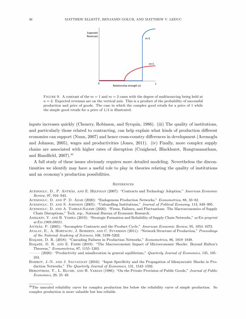
36 MATTHEW ELLIOTT, BENJAMIN GOLUB, AND MATTHEW V. LEDUC
m=2
Relationship strength (s)
Expected Revenues
10
m=1
Figure 9. A contrast of the m = 1 and m = 2 cases with the degree of multisourcing being held atn = 2. Expected revenues are on the vertical axis. This is a product of the probability of successfulproduction and price of goods. The case in which the complex good retails for a price of 1 whilethe simple good retails for a price of 1/4 is illustrated.
inputs increases quickly (Chenery, Robinson, and Syrquin, 1986). (iii) The quality of institutions,
and particularly those related to contracting, can help explain what kinds of production different
economies can support (Nunn, 2007) and hence cross-country differences in development (Acemoglu
and Johnson, 2005), wages and productivities (Jones, 2011). (iv) Finally, more complex supply
chains are associated with higher rates of disruption (Craighead, Blackhurst, Rungtusanatham,
and Handfield, 2007).46
A full study of these issues obviously requires more detailed modeling. Nevertheless the discon-
tinuities we identify may have a useful role to play in theories relating the quality of institutions
and an economy’s production possibilities.
References
Acemoglu, D., P. Antras, and E. Helpman (2007): “Contracts and Technology Adoption,” American EconomicReview, 97, 916–943.
Acemoglu, D. and P. D. Azar (2020): “Endogenous Production Networks,” Econometrica, 88, 33–82.Acemoglu, D. and S. Johnson (2005): “Unbundling Institutions,” Journal of Political Economy, 113, 949–995.Acemoglu, D. and A. Tahbaz-Salehi (2020): “Firms, Failures, and Fluctuations: The Macroeconomics of Supply
Chain Disruptions,” Tech. rep., National Bureau of Economic Research.Amelkin, V. and R. Vohra (2019): “Strategic Formation and Reliability of Supply Chain Networks,” arXiv preprint
arXiv:1909.08021.Antras, P. (2005): “Incomplete Contracts and the Product Cycle,” American Economic Review, 95, 1054–1073.Atalay, E., A. Hortacsu, J. Roberts, and C. Syverson (2011): “Network Structure of Production,” Proceedings
of the National Academy of Sciences, 108, 5199–5202.Baqaee, D. R. (2018): “Cascading Failures in Production Networks,” Econometrica, 86, 1819–1838.Baqaee, D. R. and E. Farhi (2019): “The Macroeconomic Impact of Microeconomic Shocks: Beyond Hulten’s
Theorem,” Econometrica, 87, 1155–1203.——— (2020): “Productivity and misallocation in general equilibrium,” Quarterly Journal of Economics, 135, 105–
163.Barrot, J.-N. and J. Sauvagnat (2016): “Input Specificity and the Propagation of Idiosyncratic Shocks in Pro-
duction Networks,” The Quarterly Journal of Economics, 131, 1543–1592.Bergstrom, T., L. Blume, and H. Varian (1986): “On the Private Provision of Public Goods,” Journal of Public
Economics, 29, 25–49.
46The unscaled reliability curve for complex production lies below the reliability curve of simple production. Socomplex production is more valuable but less reliable.

37
Bernstein, L. (1992): “Opting Out of the Legal System: Extralegal Contractual Relations in the Diamond Industry,”The Journal of Legal Studies, 21, 115–157.
Bimpikis, K., O. Candogan, and S. Ehsani (2019a): “Supply Disruptions and Optimal Network Structures,”Management Science, 65, 5504–5517.
Bimpikis, K., S. Ehsani, and R. Ilkılıc (2019b): “Cournot Competition in Networked Markets,” ManagementScience, 65, 2467–2481.
Blanchard, O. and M. Kremer (1997): “Disorganization,” The Quarterly Journal of Economics, 112, 1091–1126.
Blume, L., D. Easley, J. Kleinberg, R. Kleinberg, and E. Tardos (2011): “Network Formation in the Presenceof Contagious Risk,” in Proceedings of the 12th ACM Conference on Electronic Commerce, ACM, 1–10.
Boehm, C. E., A. Flaaen, and N. Pandalai-Nayar (2019): “Input Linkages and the Transmission of Shocks:Firm-Level Evidence from the 2011 Tohoku Earthquake,” Review of Economics and Statistics, 101, 60–75.
Boehm, J. and E. Oberfield (2020): “Misallocation in the Market for Inputs: Enforcement and the Organizationof Production,” Quarterly Journal of Economics, forthcoming.
Brummitt, C. D., K. Huremovic, P. Pin, M. H. Bonds, and F. Vega-Redondo (2017): “Contagious Disruptionsand Complexity Traps in Economic Development,” Nature Human Behaviour, 1, 665.
Buldyrev, S. V., R. Parshani, G. Paul, H. E. Stanley, and S. Havlin (2010): “Catastrophic Cascade ofFailures in Interdependent Networks,” Nature, 464, 1025.
Cabrales, A., P. Gottardi, and F. Vega-Redondo (2017): “Risk Sharing and Contagion in Networks,” TheReview of Financial Studies, 30, 3086–3127.
Carvalho, V. M., M. Nirei, Y. U. Saito, and A. Tahbaz-Salehi (2020): “Supply Chain Disruptions: Evidencefrom the Great East Japan Earthquake,” University of Cambridge.
Carvalho, V. M. and A. Tahbaz-Salehi (2019): “Production networks: A primer,” Annual Review of Economics,11, 635–663.
Carvalho, V. M. and N. Voigtlander (2014): “Input Diffusion and the Evolution of Production Networks,”Tech. rep., National Bureau of Economic Research.
Chenery, H. B., S. Robinson, and M. Syrquin (1986): Industrialization and Growth, world Bank Washington.Ciccone, A. (2002): “Input Chains and Industrialization,” The Review of Economic Studies, 69, 565–587.Craighead, C. W., J. Blackhurst, M. J. Rungtusanatham, and R. B. Handfield (2007): “The Severity of
Supply Chain Disruptions: Design Characteristics and Mitigation Capabilities,” Decision Sciences, 38, 131–156.Dasaratha, K. (2021): “Innovation and Strategic Network Formation,” Review of Economic Studies, forthcoming.Datta, P. (2017): “Supply Network Resilience: a Systematic Literature Review and Future Research,” The Inter-
national Journal of Logistics Management.Elliott, M. and B. Golub (2021): “Networks and economic fragility,” .Elliott, M., B. Golub, and M. O. Jackson (2014): “Financial Networks and Contagion,” American Economic
Review, 104, 3115–53.Elliott, M., J. Hazell, and C.-P. Georg (2018): “Systemic Risk-Shifting in Financial Networks,” Available at
SSRN 2658249.Erol, S. (2018): “Network Hazard and Bailouts,” Available at SSRN 3034406.Erol, S., F. Parise, and A. Teytelboym (2020): “Contagion in Graphons,” Available at SSRN.Erol, S. and R. Vohra (2018): “Network Formation and Systemic Risk,” Available at SSRN 2546310.Fafchamps, M. (2002): “Spontaneous Market Emergence,” Topics in Theoretical Economics, 2.Fafchamps, M. and B. Minten (1999): “Relationships and Traders in Madagascar,” The Journal of Development
Studies, 35, 1–35.Gabaix, X. (2011): “The Granular Origins of Aggregate Fluctuations,” Econometrica, 79, 733–772.Gale, D. and S. Kariv (2009): “Trading in Networks: A Normal Form Game Experiment,” Americal Economic
Journal: Microeconomics, 1, 114–132.Goyal, S. (2017): “Networks and markets,” in Advances in Economics and Econometrics: Volume 1: Eleventh
World Congress, Cambridge University Press, vol. 58, 215.Graddy, K. (2006): “Markets: the Fulton Fish Market,” Journal of Economic Perspectives, 20, 207–220.Granovetter, M. (1973): “The Strength of Weak Ties,” American Journal of Sociology, 78, 1360–1380.——— (1985): “Economic Action and Social Structure: the Problem of Embeddedness,” American Journal of
Sociology, 91, 481–510.Hall, R. E. (1979): “A Theory of the Natural Unemployment Rate and the Duration of Employment,” Journal of
Monetary Economics, 5, 153–169.Hendricks, K. B. and V. R. Singhal (2003): “The Effect of Supply Chain Glitches on Shareholder Wealth,”
Journal of operations Management, 21, 501–522.——— (2005a): “Association between Supply Chain Glitches and Operating Performance,” Management Science,
51, 695–711.——— (2005b): “An Empirical Analysis of the Effect of Supply Chain Disruptions on Long-Run Stock Price Perfor-
mance and Equity Risk of the Firm,” Production and Operations Management, 14, 35–52.
38 MATTHEW ELLIOTT, BENJAMIN GOLUB, AND MATTHEW V. LEDUC
Jackson, M. O. (2008): Social and Economic Networks, Princeton University Press.Jackson, M. O. and A. Pernoud (2019): “What Makes Financial Networks Special? Distorted Investment Incen-
tives, Regulation, and Systemic Risk Measurement,” Distorted Investment Incentives, Regulation, and SystemicRisk Measurement (March 1, 2019).
Jackson, M. O., T. Rodriguez-Barraquer, and X. Tan (2012): “Social Capital and Social Quilts: NetworkPatterns of Favor Exchange,” American Economic Review, 102, 1857–97.
Jones, C. I. (2011): “Intermediate Goods and Weak Links in the Theory of Economic Development,” AmericanEconomic Journal: Macroeconomics, 3, 1–28.
Jovanovic, B. (1987): “Micro Shocks and Aggregate Risk,” The Quarterly Journal of Economics, 102, 395–409.Kirman, A. P. and N. J. Vriend (2000): “Learning to be Loyal. A Study of the Marseille Fish Market,” in
Interaction and Market structure, Springer, 33–56.Konig, M. D., A. Levchenko, T. Rogers, and F. Zilibotti (2019): “Aggregate Fluctuations in Adaptive
Production Networks,” Tech. rep., Mimeo.Kranton, R. E. and D. F. Minehart (2001): “A theory of Buyer-Seller Networks,” American Economic Review,
91, 485–508.Kremer, M. (1993): “The O-ring Theory of Economic Development,” The Quarterly Journal of Economics, 108,
551–575.Leontief, W. W. (1936): “Quantitative Input and Output Relations in the Economic Systems of the United States,”
The Review of Economic Statistics, 105–125.Levchenko, A. A. (2007): “Institutional Quality and International Trade,” The Review of Economic Studies, 74,
791–819.Levine, D. (2012): “Production Chains,” Review of Economic Dynamics, 15, 271–282.Liu, E. (2019): “Industrial Policies in Production Networks*,” The Quarterly Journal of Economics, 134, 1883–1948.McLain, S. (2021): “Auto Makers Retreat From 50 Years of ‘Just in Time’ Manufacturing,” Wall Street Journal.McLain, S., Matthews, C. M., and C. Paris (2021): “Everywhere You Look, the Global Supply Chain Is a Mess,”
Wall Street Journal.Murdoch, J., T. Marsden, and J. Banks (2000): “Quality, Nature, and Embeddedness: Some Theoretical
Considerations in the Context of the Food Sector,” Economic Geography, 76, 107–125.Murphy, K. M., A. Shleifer, and R. W. Vishny (1989): “Industrialization and the big push,” Journal of political
economy, 97, 1003–1026.Nishiguchi, T. (1994): Strategic Industrial Sourcing: The Japanese advantage, Oxford University Press on Demand.Norrman, A. and U. Jansson (2004): “Ericsson’s Proactive Supply Chain Risk Management Approach After
a Serious sub-Supplier Accident,” International Journal of Physical Distribution & Logistics Management, 34,434–456.
Nunn, N. (2007): “Relationship-Specificity, Incomplete Contracts, and the Pattern of Trade,” The Quarterly Journalof Economics, 122, 569–600.
Oberfield, E. (2018): “A Theory of Input-Output Architecture,” Econometrica, 86.Okuno-Fujiwara, M. (1988): “Interdependence of industries, coordination failure and strategic promotion of an
industry,” Journal of International Economics, 25, 25–43.Petersen, M. A. and R. G. Rajan (1994): “The Benefits of Lending Relationships: Evidence from Small Business
Data,” The Journal of Finance, 49, 3–37.——— (1995): “The Effect of Credit Market Competition on Lending Relationships,” The Quarterly Journal of
Economics, 110, 407–443.Rodrik, D. (1996): “Coordination failures and government policy: A model with applications to East Asia and
Eastern Europe,” Journal of International Economics, 40, 1–22.Rosenstein-Rodan, P. N. (1943): “Problems of industrialisation of eastern and south-eastern Europe,” The eco-
nomic journal, 53, 202–211.Rostek, M. and M. Weretka (2015): “Dynamic Thin Markets,” The Review of Financial Studies, 28, 2946–2992.Sadler, E. (2020): “Diffusion Games,” American Economic Review, 110, 225–270.Scheinkman, J. A. and M. Woodford (1994): “Self-Organized Criticality and Economic Fluctuations,” The
American Economic Review Paper and Proceedings, 84, 417–421.Slutsken, H. (2018): “Four million parts, 30 countries: How an Airbus A380 comes together,” CNN.Snyder, L. V., Z. Atan, P. Peng, Y. Rong, A. J. Schmitt, and B. Sinsoysal (2016): “OR/MS Models for
Supply Chain Disruptions: A Review,” IIE Transactions, 48, 89–109.Supply Chain Quarterly (2018): “Supply Chain Disruptions Hit Record High,” Supply Chain Quarterly, https:
//www.supplychainquarterly.com/news/20181210-supply-chain-disruptions-hit-record-high/.Talamas, E. and R. Vohra (2020): “Go Big or Go Home: A Free and Perfectly Safe but Only Partially Effective
Vaccine Can Make Everyone Worse Off,” Games and Economic Behavior, 122, 277–289.Tang, L., K. Jing, J. He, and H. E. Stanley (2016): “Complex Interdependent Supply Chain Networks: Cascading
Failure and Robustness,” Physica A: Statistical Mechanics and its Applications, 443, 58–69.

39
The Economist (2006): “When the Chain Breaks,” .Tintelnot, F., A. K. Kikkawa, M. Mogstad, and E. Dhyne (2018): “Trade and Domestic Production Networks,”
Tech. rep., National Bureau of Economic Research.Uzzi, B. (1997): “Social Structure and Competition in Interfirm Networks: The Paradox of Embeddedness,” Admin-
istrative Science Quarterly, 35–67.Yang, Q., C. Scoglio, and D. Gruenbacher (2019): “Discovery of a Phase Transition Behavior for Supply Chains
against Disruptive Events,” arXiv preprint arXiv:1908.02616.
Appendix A. Formal construction of the supply network
We now formally construct the random supply network which was introduced in Sections 2.1 and 2.2; thisconstruction provides the foundation for calculating the set of functional firms, etc.
Endow each Vi with the Borel σ-algebra and a scaling of Lebesge measure, denoted λ, and let V be thedisjoint union of these spaces, with total measure 1. Fix positive integers m and n, as well as a distribution µover the nonnegative integers. A (symmetric) potential supply network with parameters m, n, µ is a randomgraph G = (V, E) satisfying the following properties.
• Its nodes are the set V.• Edges are ordered pairs (v, v′) where v′ = (j, f ′) for j ∈ I(i)—the meaning is that v can potentially
source from v′. We depict such an edge as an arrow from v to v′.• The measure of nodes v with d(v) = d′ is µ(d′).• Consider any v ∈ Vi with d(v) > 0.
– For each j ∈ I(i) there are n edges (v, v′) to n distinct varieties v′ ∈ Vj . For any variety, defineits neighborhood Nv = {v′ : (v, v′) ∈ E}.
– The elements of Nv ∩ Vj are independently drawn from an atomless distribution over Vj con-ditioned on d(v′) = d(v)− 1.
– For any countable set of varieties V, its neighborhoods (Nv)v∈V are independent.
Now fix relationship strengths (xv)v∈V .47 Define G′ to be a random subgraph of G in which each edgefrom a node v of positive depth is kept independently, with probability xv. More formally, define for everyedge vv′ a random variable Ovv′ ∈ {0, 1} (whether the edge is operational) such that
• P[Ovv′ = 1 | G] = xv for every vv′ ∈ G and,• for any countable subset E of edges in G, the random variables (Oe)e∈E are independent conditional
on G.
The out-neighborhood of the depth-0 varieties in G′ is⋃j∈I(i) Vj , since these can source from anyone.
A subset V ⊆ V is defined to be consistent if, for each v ∈ V the following holds: for each product j that
v = (i, f) requires as inputs (∀ j ∈ I(i)), there is an operational edge (v, v′) ∈ G′) with v′ ∈ V. There maybe many consistent sets, but by Tarki’s theorem, there will be a maximal one, V ′, which is a superset of anyother consistent set. For any given variety, this can be found by the simple iterative procedure in Section2.3.
Since any countable set of edges is independent, we can make computations about the relevant marginalprobabilities in our model (e.g., reliability of any variety) as we would if there only one tree.
Appendix B. Proofs of main results
B.1. The reliability curve: Basic precipice results. The first building block of our analysis is char-acterizing the shape of the reliability curve x 7→ ρ(x, µτ ) when τ is large (so that depths are large). InFigure 10, we reproduce Figure 3 (adding one additional panel), which will help us describe what we aredoing. First, we define a correspondence that will be central to our analysis. It is a limit of the functionsx 7→ ρ(x, µτ ), in the sense that their graphs converge to the graph of the correspondence ρ(x) as τ → ∞(see panels (A) and (B)). More formally:
Definition 5. Let ρ : [0, 1] ⇒ [0, 1] be a correspondence such that48
(i) for any r ∈ ρ(x), there is a sequence {xτ}∞τ=1 → x such that limτ→∞ ρ(xτ , µτ ) = r;
47Here v 7→ xv is a given measurable function.48Equivalently, we can define ρ by saying that it is a correspondence such that the graphs of the functions ρ(·, µτ ) :[0, 1]→ [0, 1] converge to the graph of ρ (in the Hausdorff set-distance metric).
40 MATTHEW ELLIOTT, BENJAMIN GOLUB, AND MATTHEW V. LEDUC
𝑥
1
1(a)
𝜌(𝑥)
𝑥
1
1𝑥𝑐𝑟𝑖𝑡
(b)
𝜌(𝑥)
𝑥
1
1𝑥𝑐𝑟𝑖𝑡
(c)
Figure 10. Panel (A) shows how reliability varies with the investment level x when supply chainshave a finite depth. Panel (B) shows the limit correspondence of the relationships between reliabilityr and the investment level x as the depth gets large. Panel (C) shows how reliability varies withthe investment level x for infinite depth.
(ii) for any sequence {xτ}∞τ=1 → x we have limτ→∞ ρ(xτ , µτ ) ∈ ρ(x).
We will show that this limit correspondence ρ exists and is uniquely defined, and that it has the shapesketched in panel (B): zero until some point, with a vertical rise up to a certain critical level of reliability,followed by a concave ascent to reliability 1 at x = 1. With these results in hand, this subsection willculminate in the proofs of Proposition 1 and Proposition 2.
Our main result on the reliability correspondence is:
Proposition 6 (Shape of the limit reliability correspondence ρ). Let the complexity of production be m ≥ 2and the number of potential suppliers for each input be n ≥ 2. Then there is a unique ρ satisfying Definition5, and it has the following properties. There exists an xcrit ∈ (0, 1) such that
(i) ρ(x) is single-valued for all x 6= xcrit;(ii) ρ(x) = 0 for all x < xcrit;
(iii) there is a value 0 < rcrit < 1 such that ρ(xcrit) = [0, rcrit];(iv) ρ(x) is strictly increasing in x for all x > xcrit;(v) limx↓xcrit ρ
′(x) =∞.
Sections B.1.1 and B.1.2 are devoted to proving this result. A closely related (discontinuous) function,sketched in panel (c), will play a role in this analysis, as we describe next. Once this is done, we will deducePropositions 1 and 2.
B.1.1. The reliability function with infinite depth: A tool to study ρ. In order to prove Proposition 6 it ishelpful to define and characterize some properties of a certain function ρ : [0, 1]→ [0, 1], sketched in Figure10(C). It will turn out that for all x 6= xcrit, ρ(x) = ρ(x). We define ρ(x) as the largest r solving the followingequation
r = (1− (1− xr)n)m. (6)
(For intuition, note that this is equation (2), which relates reliability at depths d and d − 1, but here withthe same reliability r on both sides. This is an intuitive condition “at depth infinity” as reliability is notdecreased by adding one layer of depth.)
Lemma 2, which is proved in Section SA1.1 of the Supplementary Appendix, identifies several key prop-erties of ρ(x).
Lemma 2. Suppose the complexity of the supply network is m ≥ 2 and there are n ≥ 1 potential inputsuppliers of each firm. For r ∈ (0, 1] define
χ(r) :=1−
(1− r 1
m
) 1n
r. (7)
Then there are values xcrit, rcrit ∈ (0, 1] such that:
41
(i) ρ(x) = 0 for all x < xcrit;(ii) ρ has a (unique) point of discontinuity at xcrit;
(iii) ρ is strictly increasing for x ≥ xcrit;(iv) the inverse of ρ on the domain x ∈ [xcrit, 1], is given by χ on the domain [rcrit, 1], where rcrit =
ρ(xcrit);(v) χ is positive and quasiconvex on the domain (0, 1];(vi) χ′(rcrit) = 0.
The proof of Lemma 2 is in Section SA1.1 of the Supplementary Appendix. While the manipulations toestablish these properties are a bit involved, they amount to studying the function ρ and the pseudo-inverseof it that we have defined, χ, using calculus. Figure 11(a) depicts χ as a function of r.49
(a) (b)
Figure 11. Panel (A) plots the function χ as r varies, and then in Panel (B) we show how switchingthe axes and taking the largest r value on the graph (corresponding to the largest solution ofequation (6)) generates ρ(x).
Recall the functions ρ(x, d): consider a depth-d tree where each firm in each tier requires m kinds of inputsand has n potential suppliers of each input. We denote by ρ(x, d) the probability of successful productionat the most-downstream node of a depth-d tree with these properties. This is defined as
ρ(x, d) = (1− (1− xρ(x, d− 1))n)m
with ρ(x, 0) = 1, since the most-upstream tier nodes obtain their inputs without the possibility of disruption.It will be useful throughout that ρ(x, d) and its derivative converge uniformly to the function ρ(x) every-
where except near xcrit. Indeed, this will direclty imply that reliability curve and the marginal returns toinvestment in our model also converge (at all points but xcrit) to their corresponding values in the “infinite-depth” model that defines ρ. The following lemma formalizes these statements.
Lemma 3.
(i) For all d ≥ 1, the function x 7→ ρ(x, d) defined for x ∈ (0, 1) is strictly increasing and infinitelydifferentiable.
(ii) On any compact set excluding xcrit, the sequence (ρ(x, d))∞d=1 converges uniformly to ρ(x).(iii) On any compact set excluding xcrit, the sequence (ρ(x, µτ ))∞τ=1 converges uniformly to ρ(x).
Proof. The sequence (ρ(·, d))∞d=1 is a monotone sequence of increasing, infinitely differentiable functions,50
converging pointwise to ρ. We know that ρ is continuous on any compact set excluding xcrit. Therefore, byDini’s theorem, the functions ρ(·, d) converge uniformly to ρ.
49Since by definition the largest r satisfying (6) is the one that determines ρ(x), it follows that the increasing part ofthe function, where r ∈ [rcrit, 1] is the part relevant for determining equilibrium reliability—see Figure 11(b), wherethe light gray branch is not part of ρ.50From eq. (2), it is clear that increasing d decreases ρ(x, d), while increasing x increases it. Differentiability isstraightforward from the iterative definition.

42 MATTHEW ELLIOTT, BENJAMIN GOLUB, AND MATTHEW V. LEDUC
Note the functions ρ(·, µτ ) are strictly increasing and infinitely differentiable, since they are the averagesof such functions. Moreover, they clearly converge pointwise to ρ(x): since all the ρ(·, d) are uniformlybounded, the vanishing probability mass on low-d realizations makes only a negligible contribution to thevalue of ρ(x, µτ ) for large τ . From this the conclusions of Lemma 3 apply equally well to the sequence offunctions (ρ(·, µτ ))∞τ=1. �
B.1.2. Proof of Proposition 6. We will now establish a close relationship between ρ and our correspondenceof interest, ρ, which will allow us to use Lemmas 2 and 3 to prove Proposition 6.
Define ρ(x) = {ρ(x)} for x 6= xcrit. By Lemma 3(iii) ρ(x, µτ ) → ρ(x) as τ → ∞ for any x 6= xcrit. ThusPart (ii) of Definition 5 is satisfied. Since ρ(x) is single-valued for x 6= xcrit, Part (i) of Definition 5 alsoholds. Lemma 2 then implies points (i), (ii), (iv) and (v) of Proposition 6.
Next, define ρ(xcrit) = [0, rcrit]. We will show that the remaining conditions of Definition 5 (thosepertaining to xcrit) also hold. First, we will check Part (i) of Definition 5 for r ∈ ρ(xcrit). For any r ∈ [0, rcrit],we can construct a sequence {xτ}∞τ=1 → xcrit such that limτ→∞ ρ(xτ , µτ ) = r. To see this, simply note thatfor any r ∈ (0, rcrit] and any τ , there is an xτ such that ρ(xτ , µτ ) = r since ρ(x, µτ ) is a continuous andincreasing function of x whose image is [0, 1]. Moreover, since for any x < xcrit, limτ→∞ ρ(x, µτ ) = 0 and forany x > xcrit there exists ε > 0 such that limτ→∞ ρ(x, µτ ) = rcrit + ε, it follows that these xτ must indeedconverge to xcrit. In the case of r = 0, there exists a sequence {xτ}∞τ=1 → xcrit such that ρ(xτ , µτ ) ↓ 0 sincefor any x < xcrit, ρ(x, µτ ) ↓ 0.
Finally, we show that every sequence {xτ}∞τ=1 → xcrit satisfies limτ→∞ ρ(xτ , µτ ) ∈ [0, rcrit] (Part (ii) ofDefinition 5). This amounts to showing that the limit is at most rcrit. Suppose otherwise, that such a limitis r′ > rcrit. Let x′ be such that ρ(x′) = r′, which exists by Lemma 2. Note for all xτ < x′, we haveρ(xτ ) < r′ − ε for some positive ε, and so ρ(xτ , µτ ) < r′ for sufficiently large τ ; this is a contradiction to thehypothesis about the limit being r′.
These claims together establish the remaining content of the claim that the ρ we have defined is the limitsatisfying Definition 5. That implies part (iii) of Proposition 6. �
B.1.3. Proof of Proposition 1 (Discontinuity in reliability) using the limit reliability correspondence. We cannow use the results established to prove the proposition about the precipice.
Part (i): The fact that ρ(x, µτ )→ 0 for x < xcrit follows from Definition 5 and Proposition 6(ii).Part (ii): From Proposition 6(iii) and (iv), it follows that ρ(x) > rcrit for any x > xcrit and thus, for τ
large enough, ρ(x, µτ ) > rcrit > 0. �
B.2. Proof of Proposition 2 (Social planner’s solution). Now we can use the properties of the relia-bility curve to prove our result on the social planner’s solution. Recall that xSP (κ, µτ ) is the set of all valuesof x maximizing the planner’s objective.
First consider the following “limit” planner’s problem, defined for x ∈ [0, 1]:
max
[h(r)− 1
κcP (x)
]subject to r ∈ ρ(x). (8)
We claim that, if δ > 0 is chosen small enough, then any solution has x /∈ [xcrit − δ, xcrit + δ]. To rule outsolutions with x ∈ [xcrit − δ, xcrit), note that by Property B and continuity of cP that the cost cP (x) ispositive in that interval (if δ is fixed at a small enough value) while ρ(x) is zero by Proposition 1, so thatx = r = 0 does better. To rule out solutions with x ∈ [xcrit, xcrit + δ], first observe that for x = xcrit, theonly r that can be a solution is r = rcrit, so we may assume the solution lies on the graph of ρ. Next, notethat if δ is chosen small enough, then for any κ, we have ρ′(x) > 1
κcP (x) in the interval [xcrit, xcrit + δ] sinceρ′(x) tends to +∞ as x ↓ xcrit by Lemma 3.
Let κcrit > 0 be the minimum value of κ such that that (8) has a solution with r > 0. This κcrit existsbecause for large enough κ we have that the maximand is positive at x = xcrit, and so there must be a solutionwith positive r; similarly, κcrit is positive since for small κ, the maximand is negative for all x ≥ xcrit.51 Bythe previous paragraph, any solution at κ = κcrit satisfies x > xcrit. Since in the domain x > xcrit, we havethat ρ(x) is concave while cP is convex, for κ ≥ κcrit there is a unique, strictly positive solution (x(κ), r(κ))
51Since cP (xcrit) > 0 and cP is convex, cP (x) > 0 for all x ≥ xcrit. Thus by making κ small enough, the costsexceed the bounded benefits. We can say “minimum” rather than “infimum” in the definition of κcrit because thecorrespondence ρ is continuous, as is cP .
43
of (8) and both x and r are increasing in κ. For κ < κcrit, we have that ρ(x) = 0 at the optimum and hencecost is zero (otherwise r = x = 0 would do better). Thus, by what we have said above,
(i) for all κ < κcrit, all solutions of (8) have x ≤ xcrit − δ, have cost equal to 0, and yield reliability 0;(ii) for all κ > κcrit, all solutions of (8) have x ≥ xcrit + δ and yield reliability r ≥ rcrit;
(iii) for κ = κcrit, all solutions of (8) are outside the interval [xcrit − δ, xcrit + δ] and reliability is either0 or strictly above rcrit.
Returning to the main model rather than the limit case above: for any κ and τ , consider the followingrewriting of the planner’s problem:
max
[h(r)− 1
κcP (x)
]subject to r = ρ(x;µτ ). (9)
For any κ, it is straightforward to deduce from the definition of the correspondence ρ that a sequence ofsolutions (x(τ), ρ(x;µτ )) of (9) must converge to a solution of (8) as τ →∞.52 Thus, choosing ε small enoughand using the convergence of ρ(x;µτ ) to ρ(x) per Definition 5 (along with the properties of ρ established inProposition 1), the conclusions of the present proposition follow. �
B.3. Best responses and equilibrium behavior: Oveview and preliminaries. Our goal now is towork toward Theorem 1 on the ordered regimes and the properties of equilibrium.
For notational convenience, when analyzing equilibria, we will multiply through all firms’ profit functionsby κ, so that a firm’s cost is c(xif−x) and its gross profit is κg(r)P (xif ; r). Note this does not change any bestresponses. We maintain this convention throughout the remainder of the proofs, and in the SupplementaryAppendix.
In Figure 12, we reproduce part of Figure 5, which will guide our analysis. Before beginning, we outlinethe plan. At a high level, it amounts to bringing the best-response curve into the picture along with theprecipice graph, and ultimately formalizing the graphical intuitions in Figure 12 concerning what happensto the best-response curve as κ moves around. Throughout, a recurring strategy is to prove a result for thegame “at the τ = ∞” limit (in a sense we make precise), and then extend the conclusion to large values ofτ , where most of the mass is on deep supply trees.
To study this τ =∞ limit, we establish some notation. First, define
P (xif ; r) = (1− (1− xifr)n)m. (10)
This is the probability with which if is able to produce, as a function of its investment choice xif given thatall its suppliers have reliability r. This is simpler than our finite-τ problem because all firms are exactlysymmetric (which is only approximately true when τ is large but finite).
Define
MB(xif ; r, κ) = κg(r)∂P (xif ; r)
∂xif(11)
MC(xif ) = c′(xif − x). (12)
These are the marginal benefit and marginal cost, respectively, to a firm of investing in relationship strengthfor the supply network “at the limit.”
A first step in the analysis is making best responses at τ = ∞ tractable by expressing them as thesolution to a first-order condition equating marginal benefits and marginal costs, which is unique undersuitable assumptions. This is done in Section B.3.1. Second, we show in Section B.3.2 that if we areinterested in equilibria that are undominated in terms of social surplus, we may focus on the higher pointsof intersection in Figure 12. Third, we show in Section B.3.3 that in the limit model, there is a uniqueintersection between the two curves above reliability rcrit, as in Figure 12(d), with the best-response curvesloping down in r, which makes the comparative statics work as in the sketches.
Together, these ingredients set up the proof of Theorem 1 in Section B.4, allowing us to formalize thegraphical intuition. The remaining subsections carry out this plan.
B.3.1. Proof of Lemma 1 (Sufficient condition for unique interior local maximum of the firm’s objective).We first study the firm’s problem “at τ = ∞.” Afterward, we establish that the same uniqueness propertyholds for large, finite τ .
52This is a version of the Theorem of the Maximum on upper hemicontinuity of optimization.
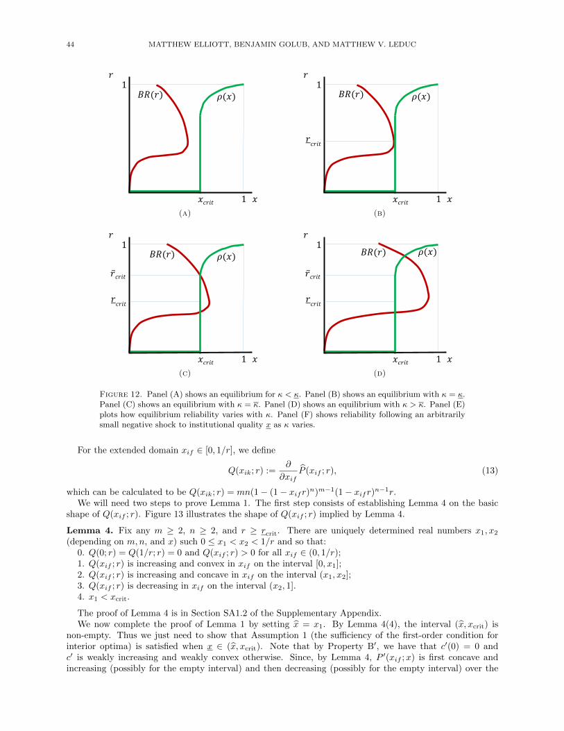
44 MATTHEW ELLIOTT, BENJAMIN GOLUB, AND MATTHEW V. LEDUC
𝑟
𝑥
1
1𝑥𝑐𝑟𝑖𝑡
𝐵𝑅(𝑟) 𝜌(𝑥)
(a)
𝑟
𝑥
1
1𝑥𝑐𝑟𝑖𝑡
𝑟𝑐𝑟𝑖𝑡
𝐵𝑅(𝑟) 𝜌(𝑥)
(b)
𝑟
𝑥
1
1
ҧ𝑟𝑐𝑟𝑖𝑡
𝑥𝑐𝑟𝑖𝑡
𝑟𝑐𝑟𝑖𝑡
𝐵𝑅(𝑟) 𝜌(𝑥)
(c)
𝑟
𝑥
1
1𝑥𝑐𝑟𝑖𝑡
𝑟𝑐𝑟𝑖𝑡
ҧ𝑟𝑐𝑟𝑖𝑡
𝐵𝑅(𝑟) 𝜌(𝑥)
(d)
Figure 12. Panel (A) shows an equilibrium for κ < κ. Panel (B) shows an equilibrium with κ = κ.Panel (C) shows an equilibrium with κ = κ. Panel (D) shows an equilibrium with κ > κ. Panel (E)plots how equilibrium reliability varies with κ. Panel (F) shows reliability following an arbitrarilysmall negative shock to institutional quality x as κ varies.
For the extended domain xif ∈ [0, 1/r], we define
Q(xik; r) :=∂
∂xifP (xif ; r), (13)
which can be calculated to be Q(xik; r) = mn(1− (1− xifr)n)m−1(1− xifr)n−1r.We will need two steps to prove Lemma 1. The first step consists of establishing Lemma 4 on the basic
shape of Q(xif ; r). Figure 13 illustrates the shape of Q(xif ; r) implied by Lemma 4.
Lemma 4. Fix any m ≥ 2, n ≥ 2, and r ≥ rcrit. There are uniquely determined real numbers x1, x2(depending on m,n, and x) such 0 ≤ x1 < x2 < 1/r and so that:
0. Q(0; r) = Q(1/r; r) = 0 and Q(xif ; r) > 0 for all xif ∈ (0, 1/r);1. Q(xif ; r) is increasing and convex in xif on the interval [0, x1];2. Q(xif ; r) is increasing and concave in xif on the interval (x1, x2];3. Q(xif ; r) is decreasing in xif on the interval (x2, 1].4. x1 < xcrit.
The proof of Lemma 4 is in Section SA1.2 of the Supplementary Appendix.We now complete the proof of Lemma 1 by setting x = x1. By Lemma 4(4), the interval (x, xcrit) is
non-empty. Thus we just need to show that Assumption 1 (the sufficiency of the first-order condition forinterior optima) is satisfied when x ∈ (x, xcrit). Note that by Property B′, we have that c′(0) = 0 andc′ is weakly increasing and weakly convex otherwise. Since, by Lemma 4, P ′(xif ;x) is first concave andincreasing (possibly for the empty interval) and then decreasing (possibly for the empty interval) over the
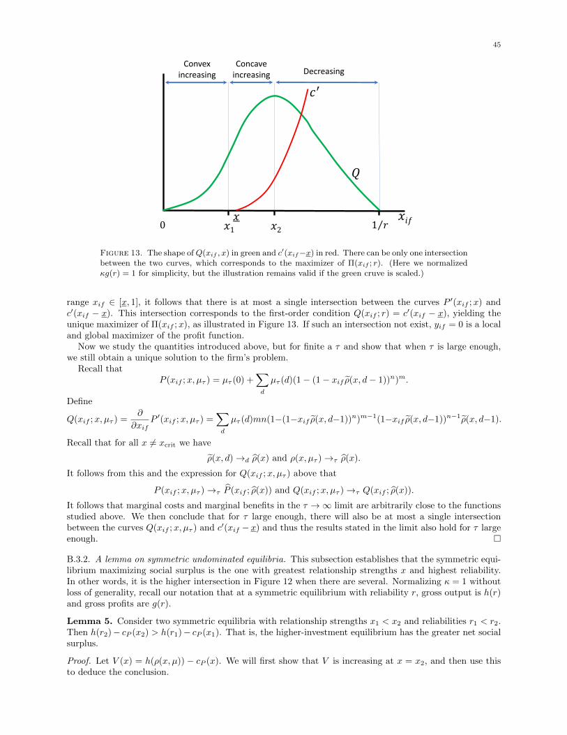
45
𝑄
Convexincreasing
Concaveincreasing Decreasing
𝑥𝑖𝑓𝑥1 𝑥20 Τ1 𝑟
𝑐′
𝑥
Figure 13. The shape ofQ(xif , x) in green and c′(xif−x) in red. There can be only one intersectionbetween the two curves, which corresponds to the maximizer of Π(xif ; r). (Here we normalizedκg(r) = 1 for simplicity, but the illustration remains valid if the green cruve is scaled.)
range xif ∈ [x, 1], it follows that there is at most a single intersection between the curves P ′(xif ;x) andc′(xif − x). This intersection corresponds to the first-order condition Q(xif ; r) = c′(xif − x), yielding theunique maximizer of Π(xif ;x), as illustrated in Figure 13. If such an intersection not exist, yif = 0 is a localand global maximizer of the profit function.
Now we study the quantities introduced above, but for finite a τ and show that when τ is large enough,we still obtain a unique solution to the firm’s problem.
Recall thatP (xif ;x, µτ ) = µτ (0) +
∑d
µτ (d)(1− (1− xif ρ(x, d− 1))n)m.
Define
Q(xif ;x, µτ ) =∂
∂xifP ′(xif ;x, µτ ) =
∑d
µτ (d)mn(1−(1−xif ρ(x, d−1))n)m−1(1−xif ρ(x, d−1))n−1ρ(x, d−1).
Recall that for all x 6= xcrit we have
ρ(x, d)→d ρ(x) and ρ(x, µτ )→τ ρ(x).
It follows from this and the expression for Q(xif ;x, µτ ) above that
P (xif ;x, µτ )→τ P (xif ; ρ(x)) and Q(xif ;x, µτ )→τ Q(xif ; ρ(x)).
It follows that marginal costs and marginal benefits in the τ →∞ limit are arbitrarily close to the functionsstudied above. We then conclude that for τ large enough, there will also be at most a single intersectionbetween the curves Q(xif ;x, µτ ) and c′(xif − x) and thus the results stated in the limit also hold for τ largeenough. �
B.3.2. A lemma on symmetric undominated equilibria. This subsection establishes that the symmetric equi-librium maximizing social surplus is the one with greatest relationship strengths x and highest reliability.In other words, it is the higher intersection in Figure 12 when there are several. Normalizing κ = 1 withoutloss of generality, recall our notation that at a symmetric equilibrium with reliability r, gross output is h(r)and gross profits are g(r).
Lemma 5. Consider two symmetric equilibria with relationship strengths x1 < x2 and reliabilities r1 < r2.Then h(r2)− cP (x2) > h(r1)− cP (x1). That is, the higher-investment equilibrium has the greater net socialsurplus.
Proof. Let V (x) = h(ρ(x, µ)) − cP (x). We will first show that V is increasing at x = x2, and then use thisto deduce the conclusion.

46 MATTHEW ELLIOTT, BENJAMIN GOLUB, AND MATTHEW V. LEDUC
Consider an outcome with firm investments xV and a reliability of r. Note that the gross profit perfunctional firm is g(r) so that the gross profit integrated across all firms (functional or nonfunctional) is
GP = rg(r).
We will write net social surplus as follows, and then split it up in to consumer and producer surplus:
V = h(r)−∫Vc(xv)dv
= [h(r)−GP] +
[GP−
∫Vc(xv)dv
]= [h(r)− rg(r)]︸ ︷︷ ︸
CS
+ PrS .
Here we define total producer surplus, PrS as gross profits net of investment costs.Now, it will be useful to have two different expressions for producer surplus, which are identically equal:
PrS1 = rg(r)−∫Vc(xv)dv (14)
PrS2 =
∫V
[Πv(xv; r)− c(xv)]dv. (15)
Now make all the variables—xv’s and r’s—functions of a parameter t, according to xv = x+ t for small t,and r is a function of the xv (and thus of t. We want to totally differentiate V in t. We claim the derivativeis positive. First consider
d
dtCS =
d
dt[h(r)− rg(r)] .
Now we turn to producer surplus. Here, we need to totally differentiate in t. The endogenous variablesare the continuum of xv’s and r:
d
dtPrS =
dr
dt· ∂∂r
PrS +dxvdt
∫V
∂
∂xvPrS .
Now, the key idea of the argument is that we use the PrS1 expression for PrS in the first summand, andthe PrS2 expression for PrS in the second summand, which is legimiate since the expressions are identicallyequal. The second expression evaluates to 0 because for a fixed v, we have
∂
∂xvPrS2 =
∂
∂xv[Πv(xv; r)− c(xv)],
which is 0 by the firm’s first-order condition.Using V = CS + PrS and our calculations above,
dV
dt=dr
dth′(r) =
d
dxρ(x, µ)h′(ρ(x, µ)).
Both factors are clearly positive, so V is increasing in t.Note that for x ≥ xcrit, we have that h is concave by Property A and increasing in x while cP (x) is convex,
soh(ρ(x, µ))− cP (x)
is single-peaked. The above argument implies both equilibria are socially inefficient, and thus social surplusis increasing in x at both of them. This combined with single-peakedness shows that the one with higherrelationship strength is more efficient. �
B.3.3. A limit uniqueness result for equilibria above rcrit. In this section we prove an important lemma thatwill be used to ensure that the relationship strengths and reliability achieved at symmetric undominatedequilibria are uniquely determined. As before, we study the “τ = ∞” model as a stepping stone to ourlarge-τ results. Visually, the lemma establishes that there is at most one intersection in Figure 12 that liesabove rcrit.
To motivate the statement, consider the question: when can there be an equilibrium outcome with r ≥ rcritfor the limit payoffs at τ = ∞? Recall the definitions of marginal benefits and marginal costs from (11)and (12) above. Under Assumption 1, an interior firm optimum is characterized by the first order condition
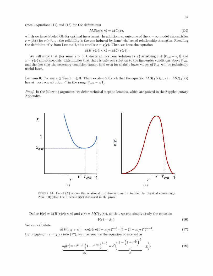
47
(recall equations (11) and (12) for the definitions)
MB(x; r, κ) = MC(x), (OI)
which we have labeled OI, for optimal investment. In addition, an outcome of the τ =∞ model also satisfiesr = ρ(x) for r ≥ rcrit: the reliability is the one induced by firms’ choices of relationship strengths. Recallingthe definition of χ from Lemma 2, this entails x = χ(r). Then we have the equation
MB(χ(r); r, κ) = MC(χ(r)).
We will show that (for some ε > 0) there is at most one solution (x, r) satisfying r ∈ [rcrit − ε, 1] andx = χ(r) simultaneously. This implies that there is only one solution to the first-order conditions above rcrit,and the fact that the necessary condition cannot hold even for slightly lower values of rcrit will be technicallyuseful later.
Lemma 6. Fix any n ≥ 2 and m ≥ 3. There exists ε > 0 such that the equation MB(χ(r); r, κ) = MC(χ(r))has at most one solution r∗ in the range [rcrit − ε, 1].
Proof. In the following argument, we defer technical steps to lemmas, which are proved in the SupplementaryAppendix.
(a) (b)
Figure 14. Panel (A) shows the relationship between r and x implied by physical consistency.Panel (B) plots the function b(r) discussed in the proof.
Define b(r) = MB(χ(r); r, κ) and c(r) = MC(χ(r)), so that we can simply study the equation
b(r) = c(r). (16)
We can calculateMB(xif ; r, κ) = κg(r)rn(1− xifr)n−1m(1− (1− xifr)n)m−1. (17)
By plugging in x = χ(r) into (17), we may rewrite the equation of interest as
κg(r)mnr2−1m
(1− r1/m
)1− 1n︸ ︷︷ ︸
b(r)
= c′( 1−
(1− r 1
m
) 1n
r︸ ︷︷ ︸x
−x). (18)

48 MATTHEW ELLIOTT, BENJAMIN GOLUB, AND MATTHEW V. LEDUC
We wish to show that there is a range [rcrit − ε, 1] for which there is at most one solution to equation(16).53 The right-hand side of the equation is increasing in r for r ∈ [rcrit, 1].54 If we could establish thatthe left-hand side, which we call b(r), is decreasing in r, it would follow that there is at most a unique rsolving (18) for r ∈ [rcrit, 1]. Moreover, by the continuity of b(r) and c(r), it would follow immediately thatfor some small ε > 0, there is also at most a single solution over the range [rcrit − ε, 1]. Unfortunately, b(r)is not decreasing in r. However, we can show that it is decreasing in r for r ≥ rcrit, which is sufficient.55
Panel (B) of Figure 14 gives a representative depiction of b(r), reflecting that it is decreasing to the right ofr (which is itself to the left of rcrit).
The following lemma will, once established, complete the proof.
Lemma 7. b is strictly decreasing on the domain [rcrit, 1).
To prove Lemma 7 we write b(r) as a product of two pieces, α(r) := κg(r) and
β(r) := mnr2−1m
(1− r 1
m
)1− 1n
.
Note that the function β(r) is positive for r ∈ (0, 1). We will show that it is also strictly decreasing on[rcrit, 1). By assumption, g(r) is positive and strictly decreasing in its argument, so α(r) is also positive anddecreasing in r. Thus, because b is the product of two positive, strictly decreasing functions on [rcrit, 1),it is also strictly decreasing on [rcrit, 1). It remains only to establish that β(r) is strictly decreasing on therelevant domain. Two additional lemmas are helpful.
Lemma 8. The function β(r) is quasiconcave and has a maximum at r :=(
(2m−1)n2mn−1
)m.
Lemma 9. For all n ≥ 2 and m ≥ 3, we have that r < rcrit.
Lemmas 8 and 9 are proved in Sections SA1.3 and SA1.4 of the Supplementary Appendix. Together theseshow that β(r) is strictly increasing and then strictly decreasing in r for r ∈ (0, 1), with a turning pointin the interval (0, rcrit). Thus β(r) is strictly decreasing on the domain [rcrit, 1), the final piece required toprove Lemma 7.
Thus, by the continuity of b(r) and c(r), it follows immediately that there exists ε > 0 such that there isat most a single solution for r ∈ [rcrit − ε, 1]. This completes the proof of the lemma. �
B.4. Proof of Theorem 1 (Classification of regimes as κ varies). Having developed the key machinerythat we will use to analyze the comparative statics of equilibria, we can proceed to the main proof. We willsometimes take x = 0 when this is immaterial to the arguments to keep notation uncluttered.
The proof relies mainly on analyzing the shape of the best-response correspondence: how it depends onκ and the reliability level r.
Denote by BR(r, κ) the set of values xif maximizing
κg(r)P (xif ; r)− c(xif − x). (19)
Recalling the definition (10), this has the interpretation of best-response relationship strengths in the infinite-depth model. Let BR(r, κ) = max{x : x ∈ BR(r, κ)} be the maximal element of the set BR(r, κ). Anal-ogously, let BR(r, κ, µτ ) = max{x : x ∈ BR(r, κ, µτ )}. This is the finite-τ analogue of the limit object wehave just defined.
Recall the optimal investment first-order condition (OI) in the limit model:
MB(x; r, κ) = MC(x), (OI)
where the definitions are in (11) and (12). We will be using it to study interior optima.A first lemma in the proof of Theorem 1 is monotonicity of the best response curve in κ.
Lemma 10. BR(r, κ) is increasing in κ, and strictly so whenever BR(r, κ) > 0.
53We note that the functions on both sides of the equation are merely constructs for the proof. In particular, whenwe sign their derivatives, these derivatives do not have an obvious economic meaning.54This follows directly: χ is increasing on that domain and c′ is increasing by assumption. (see Panel (A) of Figure14).55We do this by showing that the global maximum of b(r) is achieved at a number r that we can prove is smallerthan rcrit.

49
Proof. Let xif = BR(r, κ) and suppose OI holds at the optimum. Suppose κ increases slightly. Then,evaluated at xif , the left-hand side of OI increases and the right-hand side does not change as it does notdepend on κ. So marginal benefits exceed marginal costs at xif . Now consider increasing xif . By theassumption that c′(x′)→∞ as x′ → 1 and the boundedness of marginal benefits, there is an x′ > x so thatmarginal benefits are once again equal to marginal costs. Since the original best-response gave a nonnegativepayoff, so must x′ (since marginal benefits exceed marginal costs in moving from x to x′). By Assumption1, the first-order condition is sufficient for a best-response.
On the other hand, if BR(r, κ) = 0 is a strict best response, then by continuity of the value function, itremains so for a slightly higher κ. �
We continue with two lemmas on the best response correspondence. Thereafter, we will prove the threeclaims of the theorem.
The first lemma concerns the local comparative statics of the intersection between the graph of r 7→BR(r, κ) and the graph of ρ.
Lemma 11. Take any κ0. Consider any (x0, r0) satisfying
x = BR(r, κ) and r ∈ ρ(x) (20)
with x0 > xcrit at κ = κ0. Then there is a neighborhood around κ0 where (X(κ), R(κ)) is the unique pairsatisfying (20), and both X and R are strictly decreasing, continuous functions of κ.
Proof. Restrict attention to a neighborhood of (x0, r0) where x > xcrit and r > rcrit. Here ρ is the same asρ. Note that in the notation of Lemma 6, the the conditions (20) are equivalent to
b(r) = c(r) and x = χ(r).
The existence of continuous functions (X(κ), R(κ)) extending the solution locally follows by the implicitfunction theorem applied to this equation. The solution R(κ) can be visualized as the horizontal coordinatewhere the decreasing function b(r) in Figure 14(b) intersects the increasing function c′(χ(r) − x). As weperturb κ upward, the curve b(r) moves up pointwise. Then R(κ), the coordinate of the intersection, isincreasing in κ. The statement about X(κ) follows because X is an increasing function of R(κ) in ourneighborhood of interest. �
The following lemma concerns the convergence of the maximal best-response function BR(r, κ, µτ ) in thefinite-τ model to the limit model.
Lemma 12. BR(r, κ, µτ ) converges pointwise to BR(r, κ) for any r.
Proof of Lemma 12. When it is nonzero, BR(r, κ, µτ ) = max{x : MB(x; r, κ, µτ ) = MC(x)} where
MB(x; r, κ, µτ ) = κg(r)mn(1− xr)n−1(1− (1− xr)n)m−1r
∞∑d=1
µτ (d).
Suppose first (passing to a subsequence if necessary) we have a sequence where this these conditions hold.Note that, since µτ puts mass at least 1− 1
τ on [τ,∞), it follows that∑∞d=1 µτ (d)→ 1 as τ →∞.
It follows that, as τ →∞, we have the following convergence uniformly:
MB(x; r, κ, µτ )→ κg(r)mn(1− xr)n−1(1− (1− xr)n)m−1r = MB(x; r, κ)
and thus thatBR(r, κ, µτ )→ BR(r, κ)
for any r.When BR(r, κ, µτ ) is identically zero for each τ (again by passing to a subsequence if necessary), it
follows from uniform convergence of the firms’ value functions to their limit (19) that investing zero strictlydominates any positive level in the limit problem as well. �
We now define some key quantities that will play a role in our proof of the theorem. It is straightforwardto see by inspection of the limit maximand (19) and condition (OI) that for any r ∈ (0, 1] and any x0 < 1 ifκ is large enough, all elements of BR(r, κ) satisfy x > x0. In particular, we can guarantee that they all lieabove xcrit. What we have said implies that there is an κ1 such that for κ > κ1 the graphs of BR(r, κ) andthe graph of ρ (both viewed as sets of points (x, r)) intersect above xcrit. On the other hand, at sufficientlysmall κ, all elements of BR(r, κ) are bounded by a small number. Let κ > 0 be the smallest κ such the
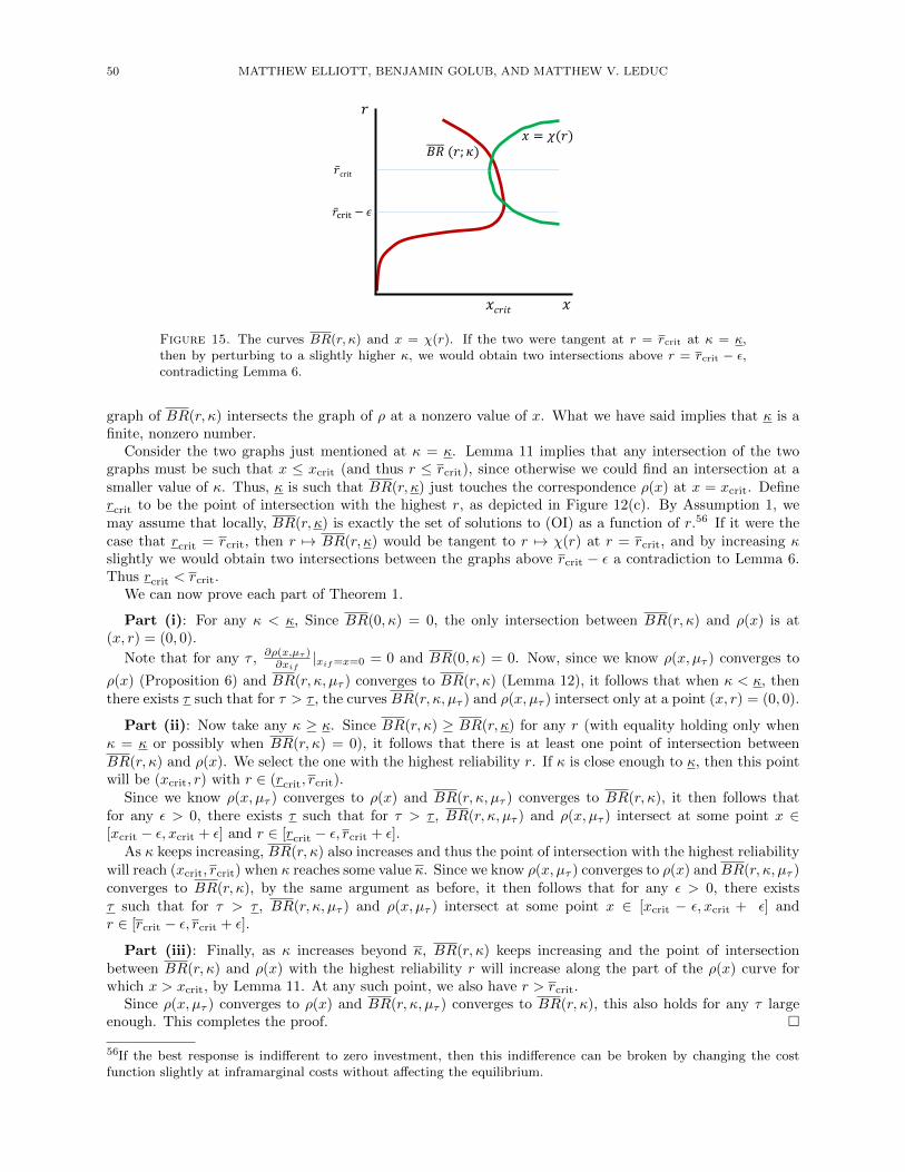
50 MATTHEW ELLIOTT, BENJAMIN GOLUB, AND MATTHEW V. LEDUC
𝑟𝑟
𝑥𝑥𝑥𝑥𝑐𝑐𝑟𝑟𝑐𝑐𝑐𝑐
��𝑟crit
𝐵𝐵𝐵𝐵 (𝑟𝑟; 𝜅𝜅)𝑥𝑥 = 𝜒𝜒(𝑟𝑟)
��𝑟crit − 𝜖𝜖
Figure 15. The curves BR(r, κ) and x = χ(r). If the two were tangent at r = rcrit at κ = κ,then by perturbing to a slightly higher κ, we would obtain two intersections above r = rcrit − ε,contradicting Lemma 6.
graph of BR(r, κ) intersects the graph of ρ at a nonzero value of x. What we have said implies that κ is afinite, nonzero number.
Consider the two graphs just mentioned at κ = κ. Lemma 11 implies that any intersection of the twographs must be such that x ≤ xcrit (and thus r ≤ rcrit), since otherwise we could find an intersection at asmaller value of κ. Thus, κ is such that BR(r, κ) just touches the correspondence ρ(x) at x = xcrit. Definercrit to be the point of intersection with the highest r, as depicted in Figure 12(c). By Assumption 1, wemay assume that locally, BR(r, κ) is exactly the set of solutions to (OI) as a function of r.56 If it were thecase that rcrit = rcrit, then r 7→ BR(r, κ) would be tangent to r 7→ χ(r) at r = rcrit, and by increasing κslightly we would obtain two intersections between the graphs above rcrit − ε a contradiction to Lemma 6.Thus rcrit < rcrit.
We can now prove each part of Theorem 1.
Part (i): For any κ < κ, Since BR(0, κ) = 0, the only intersection between BR(r, κ) and ρ(x) is at(x, r) = (0, 0).
Note that for any τ , ∂ρ(x,µτ )∂xif
|xif=x=0 = 0 and BR(0, κ) = 0. Now, since we know ρ(x, µτ ) converges to
ρ(x) (Proposition 6) and BR(r, κ, µτ ) converges to BR(r, κ) (Lemma 12), it follows that when κ < κ, thenthere exists τ such that for τ > τ , the curves BR(r, κ, µτ ) and ρ(x, µτ ) intersect only at a point (x, r) = (0, 0).
Part (ii): Now take any κ ≥ κ. Since BR(r, κ) ≥ BR(r, κ) for any r (with equality holding only whenκ = κ or possibly when BR(r, κ) = 0), it follows that there is at least one point of intersection betweenBR(r, κ) and ρ(x). We select the one with the highest reliability r. If κ is close enough to κ, then this pointwill be (xcrit, r) with r ∈ (rcrit, rcrit).
Since we know ρ(x, µτ ) converges to ρ(x) and BR(r, κ, µτ ) converges to BR(r, κ), it then follows thatfor any ε > 0, there exists τ such that for τ > τ , BR(r, κ, µτ ) and ρ(x, µτ ) intersect at some point x ∈[xcrit − ε, xcrit + ε] and r ∈ [rcrit − ε, rcrit + ε].
As κ keeps increasing, BR(r, κ) also increases and thus the point of intersection with the highest reliabilitywill reach (xcrit, rcrit) when κ reaches some value κ. Since we know ρ(x, µτ ) converges to ρ(x) and BR(r, κ, µτ )converges to BR(r, κ), by the same argument as before, it then follows that for any ε > 0, there existsτ such that for τ > τ , BR(r, κ, µτ ) and ρ(x, µτ ) intersect at some point x ∈ [xcrit − ε, xcrit + ε] andr ∈ [rcrit − ε, rcrit + ε].
Part (iii): Finally, as κ increases beyond κ, BR(r, κ) keeps increasing and the point of intersectionbetween BR(r, κ) and ρ(x) with the highest reliability r will increase along the part of the ρ(x) curve forwhich x > xcrit, by Lemma 11. At any such point, we also have r > rcrit.
Since ρ(x, µτ ) converges to ρ(x) and BR(r, κ, µτ ) converges to BR(r, κ), this also holds for any τ largeenough. This completes the proof. �
56If the best response is indifferent to zero investment, then this indifference can be broken by changing the costfunction slightly at inframarginal costs without affecting the equilibrium.
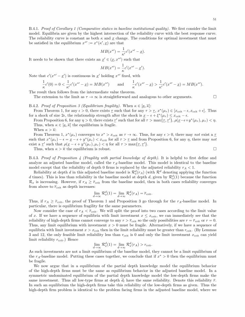
51
B.4.1. Proof of Corollary 1 (Comparative statics in baseline institutional quality). We first consider the limitmodel. Equilibria are given by the highest intersection of the reliability curve with the best response curve.The reliability curve is constant as both κ and x change. The conditions for optimal investment that mustbe satisfied in the equilibrium x∗′ := x∗(κ′, x) are that
MB(x∗′) =1
κ′c′(x∗′ − x).
It needs to be shown that there exists an x′ ∈ (x, x∗′) such that
MB(x∗′) =1
κc′(x∗′ − x′).
Note that c′(x∗′ − x′) is continuous in x′ holding x∗′ fixed, with
1
κc′(0) = 0 <
1
κ′c′(x∗′ − x) = MB(x∗′) and
1
κc′(x∗′ − x) >
1
κ′c′(x∗′ − x) = MB(x∗′).
The result then follows from the intermediate value theorem.The extension to the limit as τ →∞ is straightforward and analogous to other arguments. �
B.4.2. Proof of Proposition 3 (Equilibrium fragility). When κ ∈ [κ, κ]:From Theorem 1, for any ε > 0, there exists τ such that for any τ > τ , x∗(µτ ) ∈ [xcrit− ε, xcrit + ε]. Thus
for a shock of size 2ε, the relationship strength after the shock is x− ε+ ξ∗(µτ ) ≤ xcrit − ε.From Proposition 6, for any η > 0, there exists τ ′ such that for all τ > max{τ , τ ′}, ρ(x−ε+y∗(µτ ), µτ ) < η.Thus, when κ ∈ [κ, κ] the equilibrium is fragile.When κ > κ:From Theorem 1, x∗(µτ ) converges to x∗ > xcrit as τ →∞. Thus, for any ε > 0, there may not exist a τ
such that x∗(µτ )− ε = x− ε+ y∗(µτ ) < xcrit for all τ > τ and from Proposition 6, for any η, there may notexist a τ ′ such that ρ(x− ε+ y∗(µτ ), µτ ) < η for all τ > max{τ , τ ′}.
Thus, when κ > κ the equilibrium is robust. �
B.4.3. Proof of Proposition 4 (Fragility with partial knowledge of depth). It is helpful to first define andanalyze an adjusted baseline model, called the rA-baseline model. This model is identical to the baselinemodel except that the reliability of depth 0 firms is replaced by the adjusted reliability rA < 1.
Reliability at depth d in this adjusted baseline model is Rdx(rA) (with Rd denoting applying the functiond times). This is less than reliability in the baseline model at depth d, given by Rdx(1) because the functionRx is increasing. However, if rA ≥ rcrit from the baseline model, then in both cases reliability convergesfrom above to rcrit as depth increases:
limd→∞
Rdx(1) = limd→∞
Rdx(rA) = rcrit.
Thus, if rA ≥ rcrit, the proof of Theorem 1 and Proposition 3 go through for the rA-baseline model. Inparticular, there is equilibrium fragility for the same parameters.
Now consider the case of rA < rcrit. We will split the proof into two cases according to the limit valueof x. If we have a sequence of equilibria with limit investment x ≤ xcrit, we can immediately see that thereliability of high-depth firms cannot converge to any r > rcrit so the only possibilities are r = rcrit or r = 0.Thus, any limit equilibrium with investment x > 0 must be fragile. Alternatively, if we have a sequence ofequilibria with limit investment x > xcrit then in the limit reliability must be greater than rcrit. (By Lemmas3 and 12, the only feasible limit reliability less than rcrit is 0 and only the limit investment xcrit can yieldlimit reliability rcrit.) Hence
limd→∞
Rdx(1) = limd→∞
Rdx(rA) > rcrit.
As such investments are not a limit equilibrium of the baseline model, they cannot be a limit equilibrium ofthe rA-baseline model. Putting these cases together, we conclude that if x∗ > 0 then the equilibrium mustbe fragile.
We now argue that in a equilibrium of the partial depth knowledge model the equilibrium behaviorof the high-depth firms must be the same as equilibrium behavior in the adjusted baseline model. In asymmetric undominated equilibrium of the partial depth knowledge model the low-depth firms make thesame investment. Thus all low-type firms at depth dl have the same reliability. Denote this reliability r.In such an equilibrium the high-depth firms take this reliability of the low-depth firms as given. Thus thehigh-depth firm problem is identical to the problem facing firms in the adjusted baseline model, where we
52 MATTHEW ELLIOTT, BENJAMIN GOLUB, AND MATTHEW V. LEDUC
set rA = r and let depth d in the adjusted baseline model correspond to depth dl + d for the high-depthfirms in the partial depth knowledge model.
We thus conclude, by our analysis of the rA-adjusted baseline model, that in any symmetric undominatedequilibrium of the partial depth knowledge model if there is positive limit investment in equilibrium thenthere is also equilibrium fragility, as claimed. �
Appendix C. Microfoundations
In this appendix we use a canonical production network model with monopolistic competition to micro-found the functionality of firms, firms’ profit functions and the planner’s objective function—i.e., PropertiesA, B, B′, and C. Our goal is to keep this part of the model standard, in order to put the focus on thestructure of the underlying supply network. The proofs in Appendix B above depend on the structure ofproduction only through the properties just mentioned.
We first study production after investment has occurred and a given realized supply network is in effect;we then discuss the modeling of investment in a prior stage.
C.1. Production. In this subsection we provide a model of production that microfounds the functionalityof firms.
C.1.1. Intermediate and final versions of each variety. We let production of any variety v ∈ Vi be used inone of two ways. First it can be transformed into an intermediate good version, which is usable only bythose varieties v′ such that v ∈ PSi(v′)—i.e., the varieties v′ for which v is a potential supplier. This canbe interpreted as a costless transformation made possible by the supply relationship with v′ that makes vsuitable for use by v′. Alternatively, v can be converted costlessly into a different, consumption good version,denoted v. (As we will discuss later, this transformation technology is owned by a particular firm, whichearns rents from selling this differentiated consumption good.)
C.1.2. Quantities and production functions. Suppose v procures for its production zv,v′ units of the varietyv′ ∈ Sj(v). For a given required input j ∈ I(i), let zv,j be the total amount of j sourced by v, summingacross all of v’s suppliers for this input, and write zv for the vector of all these quantities associated withvariety v. Let `v be the amount of labor used by variety v. Labor is the only factor (i.e., unproduced good)and it is inelastically supplied, with ` = 1 unit of it. The output of v is
φv = f(`v, zv) := (`v)ε`∏j∈I(i)
(zv,j)εz , (21)
where ε` + |I(i)|εz = 1 so that there are constant returns to scale. Thus, all varieties in any set Sj(v) areperfect substitutes. Concerning substitutability across varieties, note that production is not possible if oneof the inputs cannot be sourced, but on the intensive margin different inputs are substitutable.57
Let qv be the quantity of v consumed. The household consumes aggregate gross production less in-vestments in reliability which are paid for in the aggregated final goods. Aggregate gross production of aconsumption good is given by
Y =
(∫V
(qv)ηCdv
)1/ηC
, (22)
a demand aggregator with 12 < ηC < 1.58 YC of the consumption good is allocated to consumption, while YI
is allocated to investment. Household utility is YC . Given investments, efficiency corresponds to maximizingY .
57We view the assumption that all inputs must be sourced for successful production as mild. Indeed, Boehm, Flaaen,and Pandalai-Nayar (2019) estimate, in the context of a supply network disruption event, a production function withlow elasticity of substitution, closer to Leontief than Cobb–Douglas.58The same results would hold if we defined a suitable nested-CES aggregator, with categories of products of equalmeasures being the nests. The upper bound on ηC ensures that the elasticity of substitution between varieties isfinite (so that variety is valuable), while the lower bound ensures that the equilibrium returns to increasing varietyare concave, which is technically convenient; see the discussion after Definition 1.
53
C.1.3. Functionality. Equation (21) implies that variety v ∈ Vi is able to produce if and only if it can procurequantities (zv,v′)v,v′∈V from its suppliers such that zv,j > 0 for all j ∈ I(i). This will be possible if and onlyif it has at least one link in the realized supply network to a functional supplier for each input it requires—inother words, if and only if it is functional (as defined in Section 2.3). Note that depth-zero nodes havethe same production functions as any other nodes; the only difference is that they are not reliant on theoperation of specific supply relationships, and always have a functional firm to source their inputs from.
C.2. Equilibrium on a realized supply network. We now define a competitive equilibrium and studyits structure on a realized supply network. Given a realized supply network, functional firms choose howmuch of each variety of each input to source (taking prices as given) and what price to set for its consumergood, while the representative consumer supplies a unit of labor inelastically and chooses how much of eachconsumer good variety to buy (taking prices as given). We start by considering the consumer’s problem, andthen consider firms’ problems before using these to define an equilibrium.
C.2.1. Equilibrium: Definitions. Let w denote the wage; pv the price of variety v when used as an interme-diate; and pv the price paid by the consumer for the final good corresponding to variety v. The numeraireis the price paid by the consumer for the final output.
As YI , the amount of final good devoted to investment, is sunk at the production stage, the household’sproblem is equivalent to choosing final good consumptions (qv)v to maximize equation (22) subject to thebudget constraint ∫
Vpvqvdv ≤ w +
∫V
Πvdv, (23)
where the right hand side is labor income from the consumer’s inelastically supplied unit of labor at wage wand income from the profits Πv of all firms (including those firms that are not functional). Let q∗(p) denotethe unique input bundle maximizing final good production, where p is a vector of the final good prices set bydifferent varieties, and let q∗v(p) denote the corresponding amount of variety v demanded in the productionof the final good.
Each firm takes the prices of all intermediate goods as given, as well as the final good prices of othervarieties. Prices for intermediate goods are competitive, i.e., equal to marginal costs of production.59
Our model is one of monopolistic competition in final goods: a functional firm’s problem is to choose inputquantities (zv,v′)v,v′∈V from its functional suppliers in the realized supply network, labor demand `v and aprice for its consumer good v to maximize its profits.60 We use efficient pricing for interfirm transactions tofocus on inefficiencies coming from network investment, rather than multiple-marginalization issues studiedelsewhere, but a model of this form could accommodate wedges in the interfirm prices if desired.
It is convenient to break this problem into two steps. First, for any quantity a firm produces it mustchoose its inputs to minimize its cost of production. As there are constant returns to scale, this requireschoosing inputs to minimize the cost of producing one unit and then scaling these choices up or down tomeet the production target. Thus the relative amounts of different inputs and labor used must solve
minzv,`v
∑j
∑v′∈Sj(v)
pv′zv,v′ + w`v subject to f(`v, zv) = 1 (24)
Let z∗v,v′ denote the quantity of variety v′ that v chooses to source per unit of its output, and `∗v the amountof labor that v sources per unit of its output.
Given the unit cost of production generated by solving (24), each variety v sets a price for its consumergood that maximizes its profits (taking reliability investment costs as sunk) and hence solves
maxpv
q∗v(p)[pv −∑v′
pv′z∗v,v′ − w`∗v] (25)
59Thus, the intermediate of variety v has a single price irrespective of who buys it. This pricing assumption amountsto requiring efficient production, with no distortions even when a supplier has (in a given realization) market powerover a buyer. As documented by (Uzzi, 1997; Kirman and Vriend, 2000), avoiding hold-up is an important functionof relational contracts in practice.60As in standard monopolistic competition models, a firm commits to a price pv for its consumption good v beforeproducing. These goods are sold at a markup above marginal cost; the quantity is determined by consumer demandat that price. As there are constant returns to scale, the amount of intermediate goods produced has no bearing onproduction costs for the final goods, and vice versa.
54 MATTHEW ELLIOTT, BENJAMIN GOLUB, AND MATTHEW V. LEDUC
Given a realized supply network G′ = (V, E ′), with functional firms V ′, a competitive equilibrium is givenby a specification of intermediate good production zv,v′ for all (v, v′) ∈ E ′, final good production qv for allv ∈ V ′, wage w, intermediate good price pv for all v ∈ V ′ and final good price pv for all v ∈ V ′ such that thefollowing conditions hold:
• the household is choosing how much to consume of each consumer good variety given the prices ofthese varieties to maximize its utility (22) subject to its budget constraint (23);• all functional varieties v ∈ V ′ are choosing inputs in ratios that minimize their unit cost given input
prices (solve (24));• all functional varieties v ∈ V ′ are choosing consumer good prices pv that maximize their profits given
other consumer good prices (solve (25));• markets clear (φv =
∑v′∈V′ zv,v′ + q∗v for all v ∈ V ′).
C.2.2. Equilibrium: Analysis. Equilibrium is characterized by all firms producing the same quantities of theirrespective final goods and selling these at the same price. While they affect the propagation of productionfailures, conditional on being functional local network features do not alter equilibrium prices and quantities.This can be seen by analyzing the prices of different intermediate goods. First, because of constant returnsto scale, firms sell their intermediate goods at a price equal to marginal cost. It turns out that withinan industry each functional variety is subject to the same intermediate costs, and hence sells at the sameintermediate price regardless of their depth. Second, because of the regularity of the supply network, asymmetry exists across industries which results in them selling at the same intermediate prices. Theseresults are shown formally in Lemmas 13 and 14 respectively. In Lemma 15, we show these results implythat all firms sell the same amounts to consumers at the same final prices.
Lemma 13. The selling prices pv of the intermediate goods of all varieties v ∈ Vi within any industry i areequal to some common price pi.
Proof. As there are constant returns to scale, in equilibrium each intermediate good must be sold at a priceequal to their respective marginal costs of production. Thus, by constant returns to scale, the price ofeach variety’s intermediate good, pv, does not depend on the quantity firm v produces. We establish theconclusion of the lemma by induction on the depth of the variety v. If d(v) = 0, firm v = (i, f) can sourcefrom any firm in each industry j ∈ I(i) and can thus minimize its marginal costs. It is easy to deducefrom this that pv = minf∈[0,1] p(i,f). Now take a variety v of depth d(v) = d; by definition v sources itsintermediate goods from firms with depth d − 1 in each industry j. If these produce at minimal cost so itfollows that pv = minf∈[0,1] p(i,f). This gives us that all firms in the same industry have the same marginalcosts and thus the same intermediate prices, regardless of their depth. �
Lemma 14. For any two industries i and j their intermediate prices are equal: pi = pj .
Proof. From Lemma 13, there is a price pi such that all firms in industry i sell intermediate goods at pricepi. By constant returns to scale, pi is not a function of the quantity produced and is only a function of theprices of the intermediates pj where j ∈ I(i). Moreover, each industry requires the same number of inputsand combines these with labor (at common wage w). Thus marginal cost of production for a firm and henceits price can be expressed as a function of just its intermediate good input prices pj for j ∈ I(i) and the wagew and by symmetry this is the same function for all industries. We denote this function by P; it takes as itsinput m intermediate good prices and the wage. The function is invariant to permutations of intermediategood prices. We can construct a vector of input prices for industry i as Mip, where Mi is a m×N matrixsuch that for each row r, the entry Mr,k = 0 for all k but one which we label ji(r). This index satisfiesji(r) ∈ I(i); Mr,ji(r) = 1; and Mr′,ji(r) = 0 for r′ 6= r. (The matrix simply selects, in each row, one of theinputs of industry i, and the corresponding entry of Mip corresponds to its price.) Then, for all industriesi,
pi = P(Mip;w),
The function P is weakly increasing in each input price and strictly increasing in each intermediate inputprice pj for j ∈ I(i).
Now assume, for the sake of contradiction, that not all intermediate input prices are the same. Withoutloss of generality, let pa = max{p1, ..., pN} and pb = min{p1, ..., pN} with pa
pb= r > 1. By definition, the price
of each intermediate for industry a must be at most pa, and similarly the price of each input for industry b
55
must be at least pb. Thus each element of Map must be less than or equal to each element of rMbp. Now,we claim
pa = P(Map;w) ≤ P(rMbp;w) < rP(Mbp;w) = rpb = pa.
To show the strict inequality, note that strictly increasing all intermediate prices relative to the wage leads toa substitution toward labor, making the increase in unit costs less than proportional. This is a contradiction.Thus, all industries must sell intermediate goods at the same price. �
Lemma 15. For any two functional firms, v, v′ ∈ V ′, the prices of these firms’ final goods are equal and thesame amount of each good is sold: pv = pv′ and q∗v(p) = q∗v′(p).
Proof. Recall that q∗v(p) denotes the demand of the consumer for final good v at prices p. We first calculatethe price elasticity of this demand for final good v.The consumers maximize (22) subject to the constraints of (23). Using the method of Lagrange multipliersto solve for the quantity of each variety demanded in terms of prices gives that for any two varieties v, v′,
q∗v(p)
p1/(ηC−1)v
=q∗v′(p)
p1/(ηC−1)v′
(26)
Because there is a continuum of firms, changing the price level and quantity of firm v will not affect theright-hand side of equation (26). Thus, the left-hand side of equation (26) is a constant function of pv. Upondifferentiating this function with respect to pv, we get
∂q∗v∂pv· pv −
q∗vηC − 1
= 0
Rearranging gives us that the price elasticity of demand for variety v at any price level is 1ηC−1 .
Now consider a firm’s pricing problem. Given an intermediate good price p (which by Lemmas 13 and 14is constant for all intermediate goods), there is a unique solution to the cost minimization problem of eachfirm (Equation (24)).
This marginal cost of production is independent of the quantity produced and is faced by all firms in eachindustry. Denote this marginal cost c. At a solution to this problem the firm charges a price pv that satisfiesthe Lerner condition:
pv − cpv
= − 1
εd(pv), (27)
where εd is the price elasticity of demand as a function of final good prices. Rearranging equation (27) andsubstituting the previously calculated elasticity, we have
ηCpv = c (28)
It is clear that the left-hand side is injective in pv and there is a unique profit-maximizing price that all firmschoose. Additionally, as the price elasticity of demand is constant, equation (27) implies that all firms willcharge the same constant markup regardless of the quantity of goods they are producing. �
We have shown that in equilibrium: (i) each functional variety v has the same consumer good output qv,which we will call q; (ii) these goods are all priced at the same price pv; (iii) all intermediate goods of varietyv ∈ V have the same price pv = p. There are two other features of the equilibrium that are crucial:
Lemma 16.
(1) Gross output is equal to h(ρ(x, µ)), where h : [0, 1] → R+ is an increasing and continuous functionwith bounded derivative and h(0) = 0.
(2) The expected gross profit of producing each variety, conditional on that variety being functional, isequal to g(ρ(x, µ)); where g : [0, 1]→ R+ is a decreasing function.
Proof. Note that because labor is the only unproduced input, all labor can be assigned to the production offinal goods by allocating labor used to produce intermediate goods to the final good that this intermediategood is ultimately used to produce. Let Lv be the total labor assigned in this way to the production ofvariety v’s final good. As by Lemmas 14 and 15 all firms have equivalent production functions, face thesame input prices and choose the same final good prices, they will use the same ratio of different inputs inproduction. This symmetry throughout the supply network implies that Lv = L for all varieties v. (Thisdoes not depend on depth because the zero depth producers have production functions identical to those of
56 MATTHEW ELLIOTT, BENJAMIN GOLUB, AND MATTHEW V. LEDUC
other firms and buy inputs—they can just do so from any variety without needing a specific relationship.)As there is a total supply of labor equal to one and it is supplied inelastically, the amount of labor that canbe assigned to the production of any given final good is 1/λ(V ′), where λ(V ′) is the measure of functionalfirms (and hence equal to ρ(x, µ) as the measure of firms is 1). As L units of labor are required to produceone unit of any final good, this implies that
q∗v = q∗ =1
Lλ(V ′). Y = (λ(V ′)(q∗)ηC )
1/ηC =λ(V ′)1/ηC−1
L=ρ(x, µ)1/ηC−1
L(29)
Setting
h(ρ(x, µ)) =ρ(x, µ)1/ηC−1
L,
completes the proof of part (1).It can be computed that L depends only on the constants in the production functions, and not on x,
which establishes (3).61
To compute the wage w in terms of the numeraire, we express the aggregate expenditure on final goodsin two different ways. On the one hand as the price of the aggregate consumer good has been normalizedto 1, it is simply the quantity of aggregate output as given by equation (29) On the other hand, it is theexpenditure of the consumer on all firms’ final goods, which we simplify using equation (28), and noting thatas all inputs are sold at cost all firms have a marginal cost of production equal to wL:
pv
∫V
(qv)dv = ρ(x, µ)wL
ηC
1
ρ(x, µ)L=
w
ηC
Combining these two expressions for expenditure implies that
w =(ηCL
)ρ(x, µ)
1−ηCηC .
From equation (28) each firm sets a final good price of pv = wL/ηC . Thus each firm earns gross profits(pv − c
)q∗ = w
(1− ηCηC
)1
λ(V ′)=(ηCL
)ρ(x, µ)
1−ηCηC
(1− ηCηC
)1
ρ(x, µ)=
(1− ηCL
)ρ(x, µ)
1ηC−2. (30)
This directly implies the second part of the lemma, using the fact that ηC ∈ ( 12 , 1). �
Lemma 16 provides microfoundations for Properties A and C. Setting Y (V ′) = h(ρ(x, µ)), part (1) showsthat maximized aggregate output Y (V ′) satisfies Property A. Part (2) shows that the expected gross profitfunction takes the form g(r) assumed in the model, with g(r) satisfying Property C—i.e., that g(r) is adecreasing, continuously differentiable function. For these statements it is important that L depends onlyon constants, not on x, which we have shown.
Part (2) of Lemma 16 follows from the household’s love of variety. Because of the love of variety thathouseholds have, the profit maximizing price that firms set for their consumer goods is at a markup overmarginal cost. On the other hand, constant returns to scale in the production function means that interme-diate goods that can be produced (i.e., which are able to source all of their required inputs) must be pricedat marginal cost in equilibrium. So firms’ profits depend just on the markup they charge to consumers,and the quantities they sell to consumers. When more other varieties are functional the consumer’s love ofvariety reduces demand for a given variety and hence the profits obtained by that variety.
C.3. Endogenizing relationship strengths: Efficient and equilibrium outcomes. Now we turn tothe earlier stage, before production, where firms invest in relationship strengths. Here our goal is to showhow the reduced-form modeling of investment costs that we presented in the main text (Section 4.2.2) fitsinto the general equilibrium model.
61Let ` be the amount of labor firm v directly hires to produce a unit of its final good. Let z be the amountof each intermediate firm v uses from one of its suppliers to produce a unit of its final good. By symmetry andconstant returns to scale, this firm minimizes its unit cost in terms of labor, L = `
1−mz subject to the constraint that
1 = zmεz `ε` . Solving the Lagrangian yields that for some constant γ, we have εzz
= γ`(1−mz)2 and ε`
`= γ
1−mz . Solving
this shows that at the optimum z = εz, we have ` = ε−mεz/ε`z and L = ε
−mεz/ε`zε`
.
57
C.3.1. The technology of investment. There is a technology available to each firm to invest the consumptiongood and increase relationship strengths. Before production, each firm if pledges some amount of theconsumption good to invest. We posit that it costs a firm 1
κc(xif−x) units of the numeraire (the consumptiongood) to achieve relationship strength x with its potential suppliers, where c is a given function—an exogenoustechnology of investment.
Thus, a firm’s expected profit when it is making its investment decision is
Πif = P (xif ;x, µ)g(r)− 1
κc(xif − x);
here both expected revenues and costs are in units of the numeraire. This microfounds the form of the firmprofits we have assumed.
C.3.2. Planner’s problem. We study the problem of efficiently choosing the investments in the first stage.The planner may choose any symmetric investments x for the firms. For a fixed choice of relationshipstrengths x, let h(ρ(x, µ)) denote the gross production of the aggregated consumption good. As we havesaid, household consumption is YC = Y −YI , where YI is the value of the investment in relationship strengthin terms of the quantity of the consumption good devoted to it. These are costs that are sunk prior toproduction. Obtaining reliability x for all such relationships costs the planner
YI =∑i∈I
∫v∈Vi
1
κc(x− x)dv =
1
κc(x− x).
(Recall that the measure of the set of all varieties is λ(V) = 1.) Setting cP (x) = c(x− x) the planner’s costfunction inherits the key properties of the individual cost function (it is continuous, increasing, and weaklyconvex with c(0) = 0, c′(0) = 0 and limx→1 c(x) = ∞ by Property B′) and hence satisfies the propertiesassumed in Property B.
Maximizing YC = Y − YI amounts to our planner’s problem from the main text:
maxx∈[0,1]
h(ρ(x, µ))− 1
κcP (x)