Embed Size (px)
Citation preview

FEDERAL UNIVERSITY OF CEARÁ
CENTER OF SCIENCE
DEPARTMENT OF COMPUTER SCIENCE
POST-GRADUATION PROGRAM IN COMPUTER SCIENCE
CRISTIANO SOUSA MELO
SUPPORTING CHANGE-PRONE CLASS PREDICTION
FORTALEZA
2020

CRISTIANO SOUSA MELO
SUPPORTING CHANGE-PRONE CLASS PREDICTION
Dissertation submitted to the Post-GraduationProgram in Computer Science of the Center ofScience of the Federal University of Ceará, asa partial requirement for obtaining the title ofMaster in Computer Science. ConcentrationArea: Information Systems
Advisor: Prof. Dr. José Maria da SilvaMonteiro Filho
FORTALEZA
2020

Dados Internacionais de Catalogação na Publicação Universidade Federal do Ceará
Biblioteca UniversitáriaGerada automaticamente pelo módulo Catalog, mediante os dados fornecidos pelo(a) autor(a)
M485s Melo, Cristiano Sousa. Supporting Change-Prone Class Prediction / Cristiano Sousa Melo. – 2020. 57 f. : il. color.
Dissertação (mestrado) – Universidade Federal do Ceará, Centro de Ciências, Programade Pós-Graduação em Ciência da Computação, Fortaleza, 2020. Orientação: Prof. Dr. José Maria da Silva Monteiro Filho.
1. Guideline. 2. Change-Prone Class Prediction. 3. Recurrent Algorithms. 4. Time-Series.I. Título.
CDD 005

CRISTIANO SOUSA MELO
SUPPORTING CHANGE-PRONE CLASS PREDICTION
Dissertation submitted to the Post-GraduationProgram in Computer Science of the Center ofScience of the Federal University of Ceará, asa partial requirement for obtaining the title ofMaster in Computer Science. ConcentrationArea: Information Systems
Approved on:
EXAMINATION BOARD
Prof. Dr. José Maria da Silva MonteiroFilho (Advisor)
Federal University of Ceará (UFC)
Prof. Dr. João Paulo Pordeus GomesFederal University of Ceará (UFC)
Prof. Dr. César Lincoln Cavalcante MattosFederal University of Ceará (UFC)
Prof. Dr. Gustavo Augusto Lima de CamposCeará State University (UECE)

To my family, all my friends, and my advisor.

ACKNOWLEDGEMENTS
I want to thank my parents firstly for supporting me all this time. They have always
been there for me and encouraged me to pursue my studies.
I will be forever in debt with my advisor José Maria Monteiro. He always was very
kind and supportive while I was going through a rough patch personally. I was truly fortunate to
be mentored by him.
I cannot forget two essential people who helped me to go until the end of this journey:
Roselia Machado and Javam Machado. Without them, I probably would not have finished this
important cycle in my life. Thanks for all the opportunities given to me.
My best friend Rebeca Matos Freire, who always has seen at me the potential to go
so far. She always knew which exactly words to say when I was sad (and thinking in give up).
Thanks for listening to me. Thanks for crying with me. You are the best person that I have met
in my life.
Several people helped me during this journey, and I would like to highlight Everson
Haroldo Monteiro de Oliveira. You have been taking care of me since graduation. Thanks for all
the cup of coffee (free sugar, of course), and Red Bulls.
At UFC, I was lucky to work with Matheus Mayron Lima da Cruz. He is one of the
most brilliant students I have met and an excellent friend who always has been there when I
needed some support.
I also would like to thank Felipe Timbó. He made part of an essential process, and
he was the best manager that I have had.
To my friends Francisco Bruno Gomes da Silva, Thainá Soares, Francildo Félix
Moura, João Ângelo Cândido Júnior, and Camila Mesquita Félix, for taking me off the books
and make me enjoy a lot of perfect moments with you.
This study was financed in part by the Coordenação de Aperfeiçoamento de Pessoal
de Nível Superior - Brasil (CAPES) - Programa de Demanda Social Protocol. 88882.454400/2019-
01.

ABSTRACT
During the development and maintenance of software, changes can occur due to new features,
bug fixes, code refactoring, or technological advancements. In this context, change-prone class
prediction can be very useful in guiding the maintenance team, since it is possible to focus
efforts on improving the quality of these code snippets and make them more flexible for future
changes. In this work, we have proposed a guideline to support the change-prone class prediction
problem, which deals with a set of hardworking strategies to improve the quality of the predictive
models. Besides, we have proposed two data structures that take the temporal dependencies
between these changes into account, called Concatenated and Recurrent approaches. They are
also called dynamic approaches, in contrast with the conventional state-of-art static approach.
Our experimental results have shown that the proposed dynamic approaches have had a better
Area Under the Curve (AUC) over the static approach.
Keywords: Guideline. Change-Prone Class Prediction. Time-Series. Recurrent Algorithms.

RESUMO
Durante o desenvolvimento e a manutenabilidade de um software, alterações podem ocorrer
devido a novos recursos, correções de bugs, refatoração de código ou avanços tecnológicos. Nesse
contexto, a predição de classe propensa a mudanças pode ser muito útil para orientar a equipe
de manutenção, pois é possível concentrar esforços na melhoria da qualidade desses trechos
de código e torná-los mais flexíveis para mudanças futuras. Neste trabalho, propusemos um
guideline para o problema de predição de classe propensa a mudança, que lida com um conjunto
de estratégias para melhorar a qualidade dos modelos preditivos. Além disso, propusemos duas
estruturas de dados que levam em consideração as dependências temporais entre essas mudanças,
chamadas abordagens concatenadas e recorrentes. Eles também são chamados de abordagens
dinâmicas, em contraste com o conceito estático existente do estado da arte. Nossos resultados
mostraram que as abordagens dinâmicas tiveram uma Área Sob a Curva (AUC) melhor do que a
abordagem estática.
Palavras-chave: Guideline. Predição de Classe Propensa a Mudança. Séries Temporais. Algo-
ritmos Recorrentes.

LIST OF FIGURES
Figure 1 – Phase 1: Designing the Dataset . . . . . . . . . . . . . . . . . . . . . . . . 18
Figure 2 – A single instance from the static approach. . . . . . . . . . . . . . . . . . . 21
Figure 3 – The Split Process for Window Size two. . . . . . . . . . . . . . . . . . . . 22
Figure 4 – Concatenated Structure. . . . . . . . . . . . . . . . . . . . . . . . . . . . . 23
Figure 5 – Recurrent Structure. . . . . . . . . . . . . . . . . . . . . . . . . . . . . . . 24
Figure 6 – Phase 2: Applying Change-Proneness Prediction. . . . . . . . . . . . . . . 24
Figure 7 – Splitting Dataset into Train and Test. . . . . . . . . . . . . . . . . . . . . . 25
Figure 8 – Undersampling and Oversampling Techniques. . . . . . . . . . . . . . . . . 29
Figure 9 – Evolution of Classes through Releases. . . . . . . . . . . . . . . . . . . . . 37
Figure 10 – Execution Tree of all Experimental Scenarios. . . . . . . . . . . . . . . . . 41
Figure 11 – Performance Evaluation in Different Baselines Scenarios. . . . . . . . . . . 41
Figure 12 – Comparison of the Best Results between Different Approaches. . . . . . . . 50
Figure 13 – Baselines Comparison between Different Approaches. . . . . . . . . . . . . 51

LIST OF TABLES
Table 1 – Overview of the Related Works . . . . . . . . . . . . . . . . . . . . . . . . 17
Table 2 – Taxonomy of some Feature Selection Algorithms. . . . . . . . . . . . . . . . 27
Table 3 – Descriptive Statistics. . . . . . . . . . . . . . . . . . . . . . . . . . . . . . . 38
Table 4 – Spearman’s Correlation of the Independent Variables . . . . . . . . . . . . . 39
Table 5 – Overview of the Dataset Before and After Outliers Removal. . . . . . . . . . 39
Table 6 – Feature Selection Results. . . . . . . . . . . . . . . . . . . . . . . . . . . . 40
Table 7 – Characteristics of the Apache Software Projects Used to Generate the Datasets. 45
Table 8 – Descriptive Statistics for Apache Ant. . . . . . . . . . . . . . . . . . . . . . 45
Table 9 – Descriptive Statistics for Apache Beam. . . . . . . . . . . . . . . . . . . . . 45
Table 10 – Descriptive Statistics for Apache Cassandra. . . . . . . . . . . . . . . . . . . 46
Table 11 – Best Results for each Dataset Using the Static Approach. . . . . . . . . . . . 46
Table 12 – Best Results for Different Window Size (WS) Using the Concatenated Approach. 49
Table 13 – Best Results for Different Window Size (WS) Using the Recurrent Approach. 49
Table 14 – Overview of the Related Works . . . . . . . . . . . . . . . . . . . . . . . . 51
CONTENTS
1 INTRODUCTION . . . . . . . . . . . . . . . . . . . . . . . . . . . . . . 12
2 RELATED WORKS . . . . . . . . . . . . . . . . . . . . . . . . . . . . . 15
3 A GUIDELINE TO SUPPORT CHANGE-PRONE CLASS PREDIC-
TION PROBLEM . . . . . . . . . . . . . . . . . . . . . . . . . . . . . . 18
3.1 Phase 1: Designing the Dataset . . . . . . . . . . . . . . . . . . . . . . . 18
3.1.1 Choose the Independent Variables . . . . . . . . . . . . . . . . . . . . . . 18
3.1.2 Choose the Dependent Variable . . . . . . . . . . . . . . . . . . . . . . . . 20
3.1.3 Collect Metrics . . . . . . . . . . . . . . . . . . . . . . . . . . . . . . . . . 20
3.1.4 Define the Input Data Structure . . . . . . . . . . . . . . . . . . . . . . . 20
3.1.4.1 Static Approach . . . . . . . . . . . . . . . . . . . . . . . . . . . . . . . . 21
3.1.4.2 Dynamic Approach . . . . . . . . . . . . . . . . . . . . . . . . . . . . . . . 22
3.2 Phase 2: Applying Change-Proneness Prediction . . . . . . . . . . . . . 24
3.2.1 Statistical Analyses . . . . . . . . . . . . . . . . . . . . . . . . . . . . . . 25
3.2.2 Outlier Filtering . . . . . . . . . . . . . . . . . . . . . . . . . . . . . . . . 25
3.2.3 Normalization . . . . . . . . . . . . . . . . . . . . . . . . . . . . . . . . . 26
3.2.4 Feature Selection . . . . . . . . . . . . . . . . . . . . . . . . . . . . . . . 27
3.2.5 Resample Techniques for Imbalanced Data . . . . . . . . . . . . . . . . . 28
3.2.6 Generating Models . . . . . . . . . . . . . . . . . . . . . . . . . . . . . . 30
3.2.7 Cross-Validation . . . . . . . . . . . . . . . . . . . . . . . . . . . . . . . . 30
3.2.8 Tuning the Predictive Model . . . . . . . . . . . . . . . . . . . . . . . . . 30
3.2.9 Selection of Performance Metrics . . . . . . . . . . . . . . . . . . . . . . 31
3.2.10 Ensure the Reproducibility . . . . . . . . . . . . . . . . . . . . . . . . . . 32
4 CASE STUDY I: USING THE STATIC APPROACH . . . . . . . . . . . 35
4.1 Phase 1: Designing the Dataset with Static Approach . . . . . . . . . . . 35
4.1.1 Independent Variables . . . . . . . . . . . . . . . . . . . . . . . . . . . . . 35
4.1.2 Dependent Variable . . . . . . . . . . . . . . . . . . . . . . . . . . . . . . 36
4.1.3 Collect Metrics . . . . . . . . . . . . . . . . . . . . . . . . . . . . . . . . . 36
4.1.4 Defining the Input Data Structure . . . . . . . . . . . . . . . . . . . . . . 38
4.2 Phase 2: Applying Change-Proneness Prediction using Static Approach 38
4.2.1 Statistical Analysis . . . . . . . . . . . . . . . . . . . . . . . . . . . . . . 38
4.2.2 Outlier Filtering . . . . . . . . . . . . . . . . . . . . . . . . . . . . . . . . 38

4.2.3 Normalization . . . . . . . . . . . . . . . . . . . . . . . . . . . . . . . . . 39
4.2.4 Feature Selection . . . . . . . . . . . . . . . . . . . . . . . . . . . . . . . 39
4.2.5 Resample Techniques . . . . . . . . . . . . . . . . . . . . . . . . . . . . . 40
4.2.6 Generate Models and Cross-Validation . . . . . . . . . . . . . . . . . . . . 40
4.2.7 Selecting Performance Metrics . . . . . . . . . . . . . . . . . . . . . . . . 41
4.2.8 Tuning the Prediction Model . . . . . . . . . . . . . . . . . . . . . . . . . 42
4.2.9 Ensure the Reproducibility . . . . . . . . . . . . . . . . . . . . . . . . . . 42
4.3 Discussion of Results . . . . . . . . . . . . . . . . . . . . . . . . . . . . . 42
4.4 Threats to Validity . . . . . . . . . . . . . . . . . . . . . . . . . . . . . . 43
5 CASE STUDY II: USING THE DYNAMIC APPROACHES . . . . . . . 44
5.1 Generating Baseline in Apache Dataset using Static Approach . . . . . . 44
5.1.1 Phase 1: Designing the Dataset with Static Approach . . . . . . . . . . . . 44
5.1.2 Phase 2: Applying Change-Proneness Prediction using Static Approach . 45
5.1.2.1 Overview of Baseline . . . . . . . . . . . . . . . . . . . . . . . . . . . . . 45
5.1.2.2 Baseline Results . . . . . . . . . . . . . . . . . . . . . . . . . . . . . . . . 46
5.2 Generating Baseline in Apache Dataset using Dynamic Approaches . . . 47
5.2.1 Phase 1: Designing the Dataset with Dynamic Approaches . . . . . . . . . 47
5.2.1.1 Defining the Input Data Structure . . . . . . . . . . . . . . . . . . . . . . . 47
5.2.2 Phase 2: Applying Change-Proneness Prediction using Dynamic Approaches 48
5.2.2.1 Ensure the Reproducibility . . . . . . . . . . . . . . . . . . . . . . . . . . . 49
5.2.3 Discussion of Results . . . . . . . . . . . . . . . . . . . . . . . . . . . . . 50
5.2.4 Threats to Validity . . . . . . . . . . . . . . . . . . . . . . . . . . . . . . . 52
6 CONCLUSION AND FUTURE WORKS . . . . . . . . . . . . . . . . . 53
REFERENCES . . . . . . . . . . . . . . . . . . . . . . . . . . . . . . . . 55

12
1 INTRODUCTION
Software maintenance has been regarded as one of the most expensive and arduous
tasks in the software lifecycle, according to Koru and Liu (2007). Software systems evolve in
response to the world’s changing needs and requirements. So, a change could occur due to the
existence of bugs, new features, code refactoring, or technological advancements. As the systems
evolve from a release to the next, Koru and Liu (2007) have observed they become larger and
more complex. Besides, Elish and Al-Khiaty (2013) highlight that managing and controlling
change in software maintenance is one of the most critical concerns of the software industry. As
software systems evolve, focusing on all of their parts of the same way is hard and a waste of
resources.
In this context, Elish et al. (2015) observe that a change-prone class is likely to
change with a high probability after a new software release. Then, it can represent the weak part
of a system. Therefore, change-prone class prediction can be beneficial and helpful in guiding the
maintenance team, distributing resources more efficiently, and thus, enabling project managers
to focus their effort and attention on these classes during the software evolution process. For
instance, refactoring can emphasize change-prone classes to improve their quality and make
them more flexible in order to better accommodate future changes and to localize the impact of
changing them. Inspection and testing activities can stress such classes, and thus enable efficient
allocation of precious resources.
In order to predict change-prone classes, different categories of software metrics
have been proposed by different authors, such as Oriented Object metrics by Chidamber and
Kemerer (1994), Code Smells by Khomh et al. (2009), Design Patterns by Posnett et al. (2011),
and Evolution Metrics by Elish and Al-Khiaty (2013). Based on these metrics, some works
which use machine learning techniques have been proposed for building change-prone class
prediction models, such as Bayesian Networks by Koten and Gray (2006), Neural Networks by
Amoui et al. (2009), and Ensemble methods by Elish et al. (2015). A typical prediction model
based on machine learning is designed by learning from historical labeled data within a project
in a supervised way.
However, despite the flexibility of emerging Machine Learning techniques, owing to
its intrinsic mathematical and algorithmic complexity, they have often considered a “black magic”
that requires a delicate balance of a large number of conflicting factors. This fact, together with
the short description of data sources and modeling process, makes research results reported in

13
many works hard to interpret. It is not rare to see potentially mistaken conclusions drawn from
methodologically unsuitable studies. Most pitfalls of applying machine learning techniques to
predict change-prone classes originate from a small number of common issues, including data
leakage and overfitting.
Nevertheless, these traps can be avoided by adopting a suitable set of guidelines.
The term guideline is defined as a recommendation that leads or directs a course of action to
achieve a specific goal. Therefore, guidelines summarize expert knowledge as a collection
of design judgments, rationales, and principles. Despite the several works that use Machine
Learning techniques to predict change-prone classes, no significant work was done so far to
assist a software engineer in selecting a suitable process for this particular problem.
Besides, in state-of-art, the change-prone class prediction is a problem in which its
structure is a time-series since their releases are available in different period. However, this
information is not part of the scenario when the predictive models are generated. Thus, to the best
of the authors’ knowledge, although many works are studying the change-prone class prediction
problem, none of them take the temporal dependence between the instances in the datasets into
account.
In this work, besides presenting a guideline in order to generate predictive models,
we also present two approaches in order to build the datasets: (i) static and (ii) dynamic. The
former means that each instance from the dataset is taken into account to generate predictive
models individually, while the latter means there is a temporal dependence between the instances.
To validate the proposed guideline and the novel dynamic approaches, we have performed two
case studies. In the first case study, we have performed the guideline over an imbalanced dataset
called Control of Merchandise (Coca) following the static approach. Coca has extracted from
extensive commercial software, containing 8 static object-oriented metrics proposed by C&K and
McCabe. In the second case study, we wanted to investigate the gain of the AUC using dynamic
approaches over the static. For this, firstly, we have collected three Apache datasets (Ant, Beam,
and Cassandra), and we have generated their baselines in the static approach, following some
steps from the guideline. After that, we have built them in the Concatenated and Recurrent
approaches for three different window sizes.
The main contributions of this work are:
1. A guideline to support change-prone class prediction problem to standardize a minimum
list of activities and roadmaps for better generating of predictive models.

14
2. Four public datasets based on commercial software and open-source Apache projects.
3. Two novel structures involving time-series in the dataset in order to improve the quality of
the generated models.
4. Two case studies, evaluating the proposed guideline and the novel time-series approaches
in change-prone class prediction.
As a result of this work, we have had two main publications: the first one was related
to the proposed guideline in the first case study in Melo et al. (2019), and the second publication
is related to the second case study, which proposes two novel dynamic structures, in Melo et al.
(2020). Besides, we have had the third publication in Martins et al. (2020) in which we applied
the guideline in order to investigate code smells and static metrics as independent variables
empirically.

15
2 RELATED WORKS
Elish and Al-Khiaty (2013) propose and validate a set of evolution-based metrics as
potential indicators of change-proneness of the classes. Then, they have evaluated their proposed
metrics empirically as independent variables of the change-proneness of an OO system when
moving from its current release to next. The datasets used in their experiments are VSSPLUGIN
and PeerSim, from the open-source software SourceForge. To evaluate these proposed metrics,
release-by-release, these models were built in four different ways using multivariate logistic
regression analysis: (1) using both the evolution-based and C&K metrics as independent variables,
(2) using only the evolution-based metrics as independent variables, (3) using only C&K metrics
as independent variables, and (4) using only the internal class probability of changes metrics
as an independent variable. In their experiments, the authors have concluded that the inclusion
of both the proposed evolution-based metrics and the C&K metrics in a prediction model for
change-proneness do offer improved prediction accuracy compared with a model that only
includes C&K metrics, evolution-based metrics, or internal class probability. However, the
authors have not mentioned any cross-validation technique to validate their models. Besides, we
do not know if their datasets are imbalanced.
Malhotra and Khanna (2014) examine the effectiveness of ten machine learning
algorithms using C&K metrics in order to predict change-proneness classes. These algorithms are
Support Vector Machine, Gene Expression Programming, Multilayer Perceptron with conjugate
learning, Group Method Data Handling Network, K-means clustering, TreeBoost, Bagging,
Naïve Bayes, J48 Decision Tree, and Random Forest. The main objective of this study was
to evaluate several ML algorithms for their effectiveness in predicting software change. They
have concluded that CBO, SLOC, and WMC are efficient predictors of change. Besides, in their
experiments, SVM is the best ML algorithm that can be used for developing change prediction
models. The authors have worked in three JAVA projects to generate their datasets, and during
the statistical analysis for each one of them shows that there is one imbalanced dataset (26%
changed classes). However, there was not any treatment as a resampling technique. Studies
involving data normalization, outlier detection, and correlation were not performed. Although
the authors of this research have explained the process to collect the independent and dependent
variables, they did not provide the scripts containing the dataset with metrics generated.
Kaur et al. (2016) study a relationship between different types of object-oriented
metrics, code smells, and change-prone classes. They argued that code smells are better predictors
16
of change-proneness compared to OO metrics. For this, they have generated a dataset from a Java
mobile application, called MOBAC. This dataset is imbalanced, then they have used resampling
techniques such as SMOTE. They have concluded that code smells are more accurate predictors
of change-proneness than static code metrics for all Machine Learning methods. Despite this
conclusion, the authors did not provide the dataset used in their experiments.
Bansal (2017) compares the performance of search-based algorithms with machine
learning algorithms constructing models related to both approaches. These metrics were collected
from two open-source Apache projects, Rave and Commons Math. The generated datasets present
imbalanced classes, 32.8% and 23.54%, respectively. The independent variables used were C&K.
However, the author identifies some strong correlations between the independent variable, and
he decided to apply Principal Component (PC) on them. In the end, the author concludes that
search-based algorithms have proved to be capable of predicting change-prone class by showing
high values of accuracy, although it is necessary a high CPU performance compared to ML
techniques. For this work, the author uses two imbalanced datasets, but he does not use any
resampling techniques. Besides, he uses accuracy to validate their result, and he does not provide
the datasets to reproducibility.
Catolino et al. (2018) analyze 20 datasets exploiting the combination of developer-
related factors (e.g., number of developers working on a class) and evolution-based metrics as
independent variables to generate predictive models. All these datasets are imbalanced; however,
the authors did not perform any resampling techniques in order to improve the performance
metric. The authors achieved the following conclusions: developer-based change prediction
models generally show good performance. The devised combined change prediction model has
an overall F-measure of 79% and outperforms the standalone baselines by up to 22%.
Choudhary et al. (2018) have proposed the use of new metrics in order to avoid
the commonly used independent variable to generate models in change-prone class prediction
problems, like C&K or evolution-based metrics. These newly proposed metrics are execution
time, frequency or method call, run time information of methods, popularity, and class depen-
dency. They have evaluated their proposed metrics in two open-source software from Warehouse
(SourceForge), called OpenClinic and OpenHospital datasets. For evaluating the performance of
the prediction model, the authors used sensitivity, specificity, and ROC Curve. In OpenClinic
dataset, the AUC improved from 0.750 to 0.925, and in the OpenHospital dataset, the AUC
improved from 0.725 to 0.915.

17
Table 1 summarizes all aforementioned related works. It illustrates the (i) main
author, (ii) the name of the dataset, (iii) the number of releases, (iv) the imbalanced rate, (v) if
there was resampling technique, (vi) if there was statistical analysis of the dataset, (vii) if there
was cross-validation, and (viii) if the dataset is available for download. In the paper written
by Catolino, we provide the minimum and maximum releases and imbalanced rate from the
20 datasets. Some information has been omitted, as an example, the imbalanced rate of the
VSSPlugin dataset, so we flagged it as unknown (unk). We highlight that almost all works do
not provide their dataset or scripts for download. Even some papers specify some version of the
software project used, their source codes are not available on the original website.
Table 1 – Overview of the Related Works
Paper Dataset Releases Imb.Rate
Res.Tech. Stats CV Availab.
2013VSSPLUGIN 13 Unk No Yes Unk NoPeerSim 9 Unk No Yes Unk No
2014DrJava 2 49% No Yes k-fold NoDSpace 2 60% No Yes k-fold NoRobocode 2 26% No Yes k-fold No
2016 MOBAC 4 Unk Yes No k-fold No
2017Rave 2 32.8% No Yes k-fold NoCommons Math 2 23.5% No Yes k-fold No
2018 +20 9-44 19%-35% No No k-fold Yes
2018OpenClinic 4 75.8% No Yes k-fold NoOpenHospital 2 5.9% No Yes k-fold No

18
3 A GUIDELINE TO SUPPORT CHANGE-PRONE CLASS PREDICTION PROB-
LEM
This chapter describes the proposed guide to support the change-prone class predic-
tion problem, published in Melo et al. (2019). It is organized into two phases: (i) designing the
dataset from software project and (ii) generating predictive models. Each one of these phases
will be detailed next.
3.1 Phase 1: Designing the Dataset
The first phase in the proposed guide aims to design and build the dataset that will
be used by the machine learning algorithms to generate predictive models for change-prone
classes. This phase, illustrated in Figure 1, encompasses the following activities: choose the
dependent variables, choose the independent variable, collect the selected metrics, and define the
data structure into static or dynamic.
Figure 1 – Phase 1: Designing the Dataset
Source: Author.
3.1.1 Choose the Independent Variables
In order to predict change-prone classes, different categories of software metrics
can be used, such as Object-Oriented (OO), McCabe’s metrics, Code Smells, Design Patterns,
and Evolution metrics. Then, the first step to design a proper dataset consists of answering the
following question “which set of metrics (features) should be chosen as input to the prediction
model?”. In other words, which independent variables to choose? The independent variables,
also known in a statistical context as regressors, represent inputs or causes, i.e., potential reasons
for a variation on the target feature (called dependent variable). So, they are used to predict

19
the target feature. It is essential to highlight that the choice of a suitable set of metrics impacts
directly in the prediction model performance. So, different metrics have been proposed in the
literature.
Chidamber and Kemerer (1994) have proposed a metric set specifically for software
systems that are developed using the object-oriented programming paradigm. These metrics are
WMC (Weighted Methods per Class), DIT (Depth of Inheritance Tree), CBO (Class Between
Object), Response for a Class (RFC), NOC (Number of Children) and LCOM (Lack of Cohesion
in Methods).
McCabe (1976) have proposed Cyclomatic Complexity (CC), and there are extended
versions of these metrics as MAX_CC (maximum values of methods in the same class), and
AVG_CC (mean values of methods in the same class) also are used.
Halstead (1977) states that software modules that are hard to read tend to be more
defect prone. He calculates the software complexity of a module by defining four critical
attributes like the Number of Operators, the Number of Operands, the Number of Unique
Operators, and the Number of Unique Operands, then derives his metrics that provide insight
about the source code complexity.
Bansiya and Davis (2002) have observed that there are metrics to model design
properties like abstraction, messaging, and inheritance, but no object-oriented design metrics
exist for several other design properties like encapsulation and composition. Furthermore, they
state that some existing metrics to measure complexity, coupling, and cohesion require almost
a full implementation, and that is why they are difficult to generate during design. So, they
define five new metrics (known as QMOOD metrics suite), which can be calculated from the
design information only. These metrics are DAM (Data Access Metric), NPM (Number of Public
Methods), MFA (Measure of Functional Abstraction), CAM (Cohesion Among Methods), and
MOA (Measure Of Aggregation).
Besides, they have proposed new additional OO metrics like FanIn (Number of
other classes that reference the class), FanOut (Number of other classes referenced by the
class), NOA (Number of Attributes), NOPA (Number of Public Attributes), NOPRA (Number
of Private Attributes), NOAI (Number of Attributes Inherited), NOM (Number of Methods),
NOPM (Number of public methods), NOPRM (Number of Private Methods), NOMI (Number
of Methods Inherited) and LOC (Lines of Code). Gyimothy et al. (2005) have shown that Lines
of Code (LOC) is one of the best metrics for fault prediction.

20
All these aforementioned metrics measure the source code related attributes of a
software product. On the other hand, process-based metrics that measure the changing nature of
the software and that are collected over a certain period can be related to developers, revisions,
and source code changes.
3.1.2 Choose the Dependent Variable
The next step consists in defining the dependent variable, which is the variable
to be predicted. Change-prone class prediction studies the alterations of a class analyzing the
difference between an old version and a more recent new version. Lu et al. (2012) define a change
of a class when there is an alteration in the number of Lines of Code (LOC). The domain of
change-prone prediction can be either labeled 0-1 to indicate whether there was some alteration
or not. Thus, following its definition, an instance from the dataset, i.e., an object-oriented class,
will be labeled as 1 if in the next release occurs alteration in its LOC independent variable, and 0
otherwise.
Besides, the dependent variable can be a probability computed by
Pi =|(L1)i|
|(L0 +L1)i|(3.1)
where Pi is a change probability of a i-th class, |(L1)i| and |(L0 +L1)i| being the
amount of labels 1 and total labels of a i-th class, respectively.
3.1.3 Collect Metrics
This step in this phase consists of collecting the metrics chosen previously (indepen-
dent and dependent variables) from a given software project. Singh et al. (2013) cite a list of
tools to collect the most common metrics according to a used Object-Oriented programming
language (JAVA, C++, or C#). As example, we can have Scitools Understand for collect indepen-
dent variables from JAVA projects or NDepends plugin in Visual Studio to collect independent
variables from C# projects.
3.1.4 Define the Input Data Structure
After choosing the independent and dependent variable, it is necessary to define the
data structure according to the predictive model that will be generated. In this case, we can have
two approaches: (i) static and (ii) dynamic. The former means that each instance from the dataset

21
is taken into account to generate predictive models individually, while the latter means there is a
temporal dependence between the instances.
The static structure is the traditional way from the used dataset to generate predictive
models in change-prone class prediction problems mentioned in Related Works, Section 2.
However, we are going to define two dynamic structures since they can improve the performance
metrics of the models over the static structure. These results can be seen in the second Case
Study, section 5.
3.1.4.1 Static Approach
In the static approach, each instance from the dataset will be taken into account
individually, i.e., each instance contains the metric values for a particular class in a specific
release as independent variables. Figure 2 illustrates an example of this structure. Note that each
line, i.e., instance, represents a class from the software project in a particular release, and its
columns contain k metrics M, i.e., independent variables, and one last column representing the
dependent variable D. Observe that in this example, the Ca class has three instances, one for
each release in which it appears. In practice, the Machine Learning algorithms use the k columns
M and the dependent variable D to generate their models, ignoring the class identifier C and
the release number R. It means this usual approach is just engaging in learn a pattern to predict
which class will suffer modification in the next release, ignoring their history, i.e., the temporal
dependence between the instances.
Figure 2 – A single instance from the static approach.
Source: Author.

22
3.1.4.2 Dynamic Approach
In the dynamic approach, we have proposed two time-series structures, called Con-
catenated and Recurrent, in order to exploit the temporal dependence between the instances to
improve the quality of the performance metrics of the predictive models. The Concatenated
structure has its temporal dimension incorporated from the presentation of versions of the input
at different times (releases, to be more specific). The Recurrent structure contains an internal
memory that is modified according to the presentation of the available patterns.
In these new time-series structures, depending on window size, each instance will
contain the total - or partial - history of the metrics values of a class, following its release order.
Thus, initially, to design a dataset according to those novel proposed approaches is necessary to
define a window size. The value of the window size parameter will be fixed and will define the
number of releases that will compose each instance. So, the window size value must be chosen
carefully. During the dataset building, if the number of releases that a certain class C appears is
less than the window size, the data about this class C will be dropped. However, the opposite is
not true. If the number of releases that a certain class C appears is greater than the window size,
the data about class C will be split, as shown in Figure 3. Note that, in Figure 3, there is a class
C that appears in three different releases. Now, suppose that the window size was set as two. In
this scenario, the data about class C will be split into two instances, i.e., from release i to release
i+1 and from release i+1 to release i+2.
Figure 3 – The Split Process for Window Size two.
Source: Author.
Concatenated Approach (CA)

23
To generate a dataset according to the Concatenated Approach is necessary, initially, to compute
the values of the k metrics for each release R in which a specific class C appears. So, this process
will produce R instances, each one with k columns. After that, for each class C, it needs to
concatenate its n sequential instances, where n is the window size, according to the split process.
Note that in this step, the produced instances will contain n ∗ k columns, as the independent
variable. For example, if a class C appears in R = 4 releases and the window size n = 3, two
instances, each one with k ∗3 columns will be generated.
Figure 4 illustrates a dataset built according to the Concatenated Approach. Note
that M represents the chosen metrics (they can be Oriented Object, Evolution, or Code Smells).
Thus, an instance in this dataset contains n∗ k columns, i.e., independent variables, respecting
the releases order i, i+1, ...,n to ensure the use of time-series information.
Figure 4 – Concatenated Structure.
Source: Author.
Recurrent Approach (RA)
The Recurrent Approach consists of storage the partial or total history into a single instance of
a class, forming a three-dimensional matrix (m, k, n), where m means the number of classes, k
means the number of metrics, and n means the window size.
Figure 5 depicts an example of the data structure used in the recurrent approach. R
represents the releases of a certain class C, and it will follow the release order i, i+1, ...,n. Each
one of these releases contains k metrics M. In short, this dataset contains m classes C, i.e, there
are m instances of window size n, where each release has k metrics. Note that if the window size
is less than the number of the release of a class C, this last one will be split, generating more
instances into the dataset.

24
Figure 5 – Recurrent Structure.
Source: Author.
3.2 Phase 2: Applying Change-Proneness Prediction
The second phase of this proposed guide aims to build change-prone class predictive
models. A prediction model is designed by learning from historical labeled data within a project
in a supervised way. Besides, this phase encompasses the activities related to the analysis of
the prediction model, performance metrics, the presentation of the results, and the ensure of the
experiments’ reproducibility. Figure 6 illustrates the activities that compose the second phase of
the proposed guide.
Figure 6 – Phase 2: Applying Change-Proneness Prediction.
Source: Author.
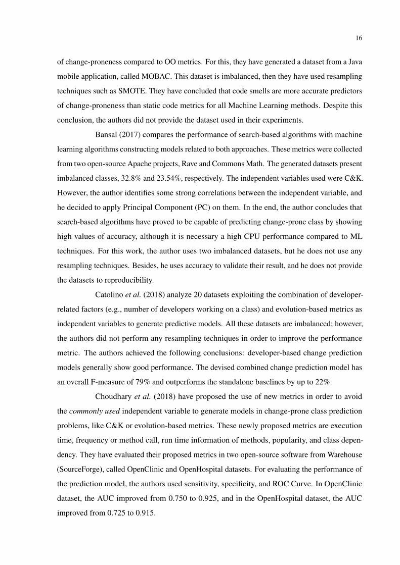
It is important to highlight that before starting to execute the guideline is essential
to split the dataset into train and test sets, according to Figure 7. The former will be performed
whole the guideline, while the latter serves to simulate the real-world data. In the case of an
25
imbalanced dataset, it is necessary to split the labels proportionally in order to avoid the bias
during the model generation. For this scenario, we recommend train_test_split function from
scikit-learn. During the cross-validation step from the guideline, the train set will be split into
train and validation sets, in order to use the test set to check the overfitting.
Figure 7 – Splitting Dataset into Train and Test.
Source: Author.
3.2.1 Statistical Analyses
Initially, a general analysis of the dataset is strongly recommended. Thus, generate
a table containing for each feature a set of valuable information, such as minimum, maximum,
mean, median (med), and standard deviation (SD) values.
After that, it is important to check the correlation between the features. Pearson’s
correlation checks the linearity between the data. It is related to the fact that the generated
prediction model may be highly biased by correlated features, then it is essential to identify those
correlations. Bishara and Hittner (2012) recommend Spearman’s correlation for nonnormally
distributed data.
3.2.2 Outlier Filtering
Outliers are extreme values that deviate from other observations on data, i.e., an
observation that diverges from an overall pattern on a sample. According to Liu et al. (2004),

26
detected outliers are candidates for aberrant data that may otherwise adversely lead to model
mispecification, biased parameter estimation, and incorrect result. It is, therefore, interesting to
identify them before create the prediction model.
We are going to cite a usual strategy to check outlier: Interquartile Range (IQR). It is
a measure of statistical dispersion, often used to detect outliers. The IQR is the length of the box
in the boxplot, i.e., Q3 - Q1. Here, outliers are defined as instances that are below Q1−1.5∗ IQR
or above Q3+1.5∗ IQR. For non-normal distribution of the dataset, Hubert and Vandervieren
(2008) suggest an IQR adaptative, since when the data are skewed, usually many points exceed
the whiskers and are often erroneously declared as outliers.
Outliers are one of the main problems when building a predictive model. Indeed,
they cause data scientists to achieve more unsatisfactory results than they could. To solve that,
we need practical methods to deal with that spurious points and remove them. If it is evident the
outlier is due to incorrectly entered or measured data, it should drop it. If the outlier does not
change the results but does affect assumptions, it also may drop the outlier. More commonly, the
outlier affects both results and assumptions. In this situation, it is not legitimate to drop it. It just
may run the analysis both with and without it. Besides, it should state how the results changed.
3.2.3 Normalization
It is essential to check if the features are on the same scale. For example, two
features A and B may have two different ranges: the first one into a range between zero and one,
meanwhile the second one is into a range in the integers domain. In this case, it is necessary to
normalize all features in the dataset. There are different strategies to normalize data. However,
it is essential to emphasize that the normalization approach must be chosen according to the
nature of the investigated problem and the used prediction algorithm. For example, Basheer and
Hajmeer (2000) have observed that for activation function in a neural network is recommended
that the data be normalized between 0.1 and 0.9 rather than 0 and 1 to avoid saturation of the
sigmoid function. Hereafter, the leading data normalization techniques are presented.
In min-max normalization features are normalized using the following equation:
x′ = λ1 +(λ2−λ1)( x−minA
maxA−minA
)(3.2)
In the equation 3.2, λ1 and λ2 are values to adjust the data domain to a desired range. For
example, to normalize the values from a dataset to [-0.3, 0.8], λ1 and λ2 must be -0.3 and 0.8,

27
respectively. The minA and maxA are the minimum and the maximum values of the feature A.
The original and the normalized value of the attribute are represented by x and x′, respectively.
The standard range is [0,1].
The z-score normalization can be computed using the following equation:
z =x−µA
σA(3.3)
In the equation 3.3, µA and σA are the mean and the standard deviation of the feature A. The
original and the normalized feature are represented by x and z, respectively. After normalization,
the mean and the standard deviation of all the features values become 0 and 1, respectively.
3.2.4 Feature Selection
According to Janecek et al. (2008), high dimensionality data is problematic for
classification algorithms due to high computational cost and memory usage. So, it is essential to
check if all features in the dataset are indeed necessary. In addition, Ladha and Deepa (2011) say
that the main benefits from feature selection techniques reduce the dimensionality space, remove
redundant, irrelevant, or noisy data and performance improvement to gain in predictive accuracy.
Table 2 – Taxonomy of some Feature Selection Algorithms.Model Search Techniques
Filter Univariate Chi-square, One-R,Information Gain
Multivariate
Correlation-basedFeature (CFS),Markov BlanketFilter (MBF)
Wrapper Deterministic
Sequential ForwardSelection (SFS),Sequential BackwardElimination (SBE)
Randomized Simulated Annealing,Genetic Algorithms
EmbeddedFeature Selection usingthe weights vectors ofSVM, Decision Trees
Source: the author.
Table 2 shows the feature selection methods in three categories: filters, wrappers,
and embedded/hybrid method. The following definitions have been presented by Veerabhadrappa
and Rangarajan (2010): Wrapper methods are brute-force feature selection, which exhaustively

28
evaluates all possible combinations of the input features and then find the best subset. Filter
methods have low computational cost but inefficient reliability in classification compared to
wrapper methods. Hybrid/ embedded methods are developed to utilize the advantages of both
filters and wrappers approaches. This strategy uses both an independent test and performance
evaluation function of the feature subset.
3.2.5 Resample Techniques for Imbalanced Data
Machine Learning techniques require an efficient training dataset, which has an
amount instances of the classes; however, as observed by Prati et al. (2009), in real-world
problems, some datasets can be imbalanced, i.e., a majority class containing most samples
meanwhile the other class contains few samples, this one generally of our interest. Using
imbalanced datasets to train models leads to higher misclassifications for the minority class. It
occurs because there is a lack of information about it.
The class imbalance problem has been encountered in multiple areas such as telecom-
munication management, bioinformatics, fraud detection, and medical diagnosis. Yang and Wu
(2006) have considered the imbalance problem as one of the top 10 problems in data mining and
pattern recognition.
In order to compute the balancing ratio (rχ ), we can use:
rχ =|χmin||χma j|
(3.4)
where χ is the dataset, | · | denotes the cardinality of a set with χmin and χma j being the subset of
samples belonging to the minority and majority class, respectively.
The state-of-the-art methods which deal with imbalanced data for classification
problems can be categorized into four groups:
Undersampling (US): it refers to the process of reducing the number of samples in
χma j. Three US known techniques are: Random Under-Sampler (RUS) proposed by Batista et al.
(2004), which consists in randomly choose an instance from the majority class and remove it;
Tomek’s Link, proposed by Tomek (1976), which consists in finding two instance, one from the
majority class and the other from the minority class, that are the nearest neighbour of each other
and then remove one of the instances; Edited Nearest Neighbours, proposed by Wilson (1972),
which consists in remove the nearest instances that do not belong to the class of the instance.
Oversampling (OS): It consists of generating synthetic data in χmin in order to

29
balance the proportion of data. Three OS known techniques are: Random Over-Sampler
(ROS), proposed by Batista et al. (2004), which consists in randomly choose an instance
from the minority class and repeat it; Synthetic Minority Oversampling Technique (SMOTE),
proposed by Chawla et al. (2002), which consists in generates new synthetic instances obtained
by combining the features of an instance and its k-nearest neighbours; Adaptive Synthetic
(ADASYN), proposed by He et al. (2008), which consists in creating synthetic instances of the
minority class considering the difficult to classify this instance with a KNN algorithm, then it
will focus on the harder instances.
The basic idea of the techniques aforementioned can be viewed in Figure 8.
Figure 8 – Undersampling and Oversampling Techniques.
Source: Author.
Combination of over and undersampling: According to Prati et al. (2009), over-
sampling can lead to overfitting, which can be avoided by applying cleaning undersampling
methods.
Ensemble learning methods: Undersampling methods imply that samples of the
majority class are lost during the balancing procedure. Ensemble methods offer an alternative to
use most of the samples. In fact, an ensemble of balanced sets is created and used to train any
classifier later.
For imbalanced multiple class classification problems, the authors Fernández et al.
(2013) have done an experimental analysis to determine the behavior of the different approaches
proposed in the specialized literature. Vluymans et al. (2017) also have proposed an extension to
multi-class data using one-vs-one decomposition.
It is essential to mention that it is necessary to separate the imbalanced dataset into
two subsets: training and test sets. After that, any of the techniques aforementioned should
only be applied in the training set because the predictive model cannot be trained with synthetic
instances.

30
3.2.6 Generating Models
When all the previous steps have been performed, it is time to generate predictive
models. In this case, a range of libraries and API software have been developed to support
this step. Scikit-learn is a free software machine learning library for the Python programming
language, proposed by Pedregosa et al. (2011), commonly used in academic research. In
addition, TensorFlow is a free and open-source software library for dataflow and differentiable
programming across a range of tasks. It is a symbolic math library and is also used for machine
learning applications such as neural networks. For API, we recommend WEKA, Waikato
Environment for Knowledge Analysis, presented by Witten et al. (1999). It is free software
licensed under the GNU General Public License.
3.2.7 Cross-Validation
Training an algorithm and evaluating its statistical performance on the same data
yields an overoptimistic result. Cross-Validation (CV) was raised to fix this issue, starting from
the remark that testing the output of the algorithm on new data would yield a reasonable estimate
of its performance. In most real applications, only a limited amount of data is available, which
leads to the idea of splitting the data: Part of data (the training sample) is used for training the
algorithm, and the remaining data (the validation sample) are used for evaluating the performance
of the algorithm. The validation sample can play the role of “new data”. As observed by Arlot
and Celisse (2010), a single data split yields a validation estimate of the risk and averaging
over several splits yields a cross-validation estimate. The significant interest of CV lies in the
universality of the data splitting heuristics.
A technique widely used to generalize the model in classification problems is k-Fold
Cross Validation. This approach divides the set in k subsets, or folds, of approximately equal
size. One fold is treated as test set meanwhile the others k−1 folds work as training set. This
process occurs k times. According to James et al. (2013), a suitable k value is k = 5 or k = 10.
3.2.8 Tuning the Predictive Model
All the steps presented in this paper so far have served to show good practicals on
how to obtain baseline according to a Machine Learning algorithm selected. Tuning it consists
of finding the best possible configuration of this algorithm at hand, wherewith best configuration.

31
It means the one that is deemed to yield the best results on the instances that the algorithm
will be eventually faced. Tuning machine learning algorithms consist of finding the best set of
hyperparameters, which yields the best results.
Hyperparameters are tuned by hand at trial-and-error procedure guided by some
rules of thumb. However, some papers analyze a set of hyperparameters for specifics algorithms in
machine learning for tuning them. For Support Vector Machine algorithm using RBF kernel, Hsu
et al. (2016) recommend a grid-search setting C = {2−5,2−3, ...,215} and γ = {2−15,2−13, ...,23}.
After defining a grid-search in a specific region, a nested cross validation must be used to
estimate the generalization error of the underlying model and its hyperparameter search. Thus,
Cawley and Talbot (2010) highlight that it makes sense to take advantage of this structure and fit
the model iteratively using a pair of nested loops, with the hyperparameters adjusted to optimize
a model selection criterion in the outer loop (model selection) and the parameters set to optimize
a training criterion in the inner loop (model fitting/training).
3.2.9 Selection of Performance Metrics
To evaluate the Machine Learning model for the classification problem is necessary
to select the appropriate performance metrics according to two possible scenarios: for a balanced
or imbalanced dataset.
A confusion matrix gives an overview of output that was sorted correctly and
incorrectly, classifying them as True Positive (TP), True Negative (TN), False Positive (FP), or
False Negative (FN).
The following metrics are widely used to validate performance results:
accuracy =T P+T N
T P+T N +FP+FN(3.5)
precision =T P
T P+FP(3.6)
recall or sensitivity =T P
T P+FN(3.7)
speci f icity =T N
T N +FP(3.8)

32
In the case of balanced datasets, such metrics (accuracy, precision, recall, and
specificity) can be used without more concerns. However, in the case of imbalanced data, these
metrics are not suitable, since they can lead to dubious results. For example, Akosa (2017) has
observed that the accuracy metric is not suitable because it tends to give a high score due to a
correct prediction of the majority class.
The Receiver Operating Characteristic (ROC) curve is a graphical plot that illus-
trates the diagnostic ability of a binary classifier system as its discrimination threshold is varied.
It is a comparison of two operating characteristics: True Positive Rate (Equation 3.7) and False
Positive Rate (Equation 3.8) as the criterion changes. The Area Under the ROC Curve (AUC)
measures the entire two-dimensional area underneath the entire ROC curve from (0,0) to (1,1).
F-score (Equation 3.9), also known as F-measure, is the harmonic average of the
precision (Equation 3.6) and recall (Equation 3.7) and its domain is [0,1]. F-score is also known
as F1-score when β value is 1.
Fβ = (1+β ) · precision · recallβ 2 · precision+ recall
(3.9)
It is essential to highlight that in the case of imbalanced data, the more suitable
metrics are AUC and F-score. These performance metrics are suitable for imbalanced data
because they take the minority classes correctly classified into account, unlike the accuracy.
3.2.10 Ensure the Reproducibility
The last step consists in to ensure the experiments reproducibility in order to verify
the credibility of the proposed study. Olorisade et al. (2017) have evaluated 30 studies in order
to highlight the difficulty of reproducing most of the works in state-of-art. While the studies
provide useful reports of their results, they lack information on access to the dataset in the form
and order as used in the original study, the software environment used, randomization control,
and the implementation of proposed techniques.
Some authors have proposed basic rules for reproducible computational research, as
Sandve et al. (2013) which list ten rules:
1. For every result, keep track of how it was produced. Whenever a result may be of potential
interest, keep track of how it was produced. When doing this, one will frequently find that
getting from raw data to the final result involves many interrelated steps (single commands,
scripts, programs).

33
2. Avoid manual data manipulation steps. Whenever possible, rely on the execution of
programs instead of manual procedures to modify data. Such manual procedures are not
only inefficient and error-prone, they are also difficult to reproduce.
3. Keep in a note the exact version of all external programs used. In order to exactly reproduce
a given result, it may be necessary to use programs in the exact versions used originally.
Also, as both input and output formats may change between versions, a newer version of a
program may not even run without modifying its inputs. Even having noted which version
was used of a given program, it is not always trivial to get hold of a program in anything
but the current version. Archiving the exact versions of programs actually used may thus
save a lot of hassle at later stages.
4. Version control all custom scripts. Even the slightest change to a computer program can
have large intended or unintended consequences. When a continually developed piece of
code (typically a small script) has been used to generate a certain result, only that exact
state of the script may be able to produce that exact output, even given the same input data
and parameters.
5. Record all intermediate results, when possible in standardized formats. In principle, as
long as the full process used to produce a given result is tracked, all intermediate data
can also be regenerated. In practice, having easily accessible intermediate results may be
of great value. Quickly browsing through intermediate results can reveal discrepancies
toward what is assumed, and can in this way uncover bugs or faulty interpretations that are
not apparent in the final results.
6. For Analysis that includes randomness, note underlying random seed. Many analyses and
predictions include some element of randomness, meaning the same program will typically
give slightly different results every time it is executed (even when receiving identical
inputs and parameters). However, given the same initial seed, all random numbers used in
an analysis will be equal, thus giving identical results every time it is run.
7. Always store raw data behind plots. From the time a figure is first generated to it being part
of a published article, it is often modified several times. In some cases, such modifications
are merely visual adjustments to improve readability, or to ensure visual consistency
between figures. If raw data behind figures are stored in a systematic manner, so as to
allow raw data for a given figure to be easily retrieved, one can simply modify the plotting
procedure, instead of having to redo the whole analysis.

34
8. Generate hierarchical analysis output, allowing layers of increasing detail to be inspected.
The final results that make it to an article, be it plots or tables, often represent highly
summarized data. For instance, each value along a curve may in turn represent averages
from an underlying distribution. In order to validate and fully understand the main result,
it is often useful to inspect the detailed values underlying the summaries. A common but
impractical way of doing this is to incorporate various debug outputs in the source code of
scripts and programs.
9. Connect textual statement to the underlying result. Throughout a typical research project,
a range of different analyses are tried and interpretation of the results made. Although the
results of analyses and their corresponding textual interpretations are clearly interconnected
at the conceptual level, they tend to live quite separate lives in their representations: results
usually live on a data area on a server or personal computer, while interpretations live in
text documents in the form of personal notes or emails to collaborators.
10. Provide public access to scripts, runs, and results. Last, but not least, all input data,
scripts, versions, parameters, and intermediate results should be made publicly and easily
accessible.
These rules are not the definitive guide of reproducibility. In some cases, such
Machine Learning for Health Care requires some particular attention in extra details, since there
are more resources to retrieve information, as an example, ECG signals and its preprocessor to
deal with this kind of data, as observed by McDermott et al. (2019).

35
4 CASE STUDY I: USING THE STATIC APPROACH
In order to evaluate the proposed guideline in Chapter 3, we have performed an
exploratory case study using 10 Machine Learning algorithms in a change-prone class dataset
called Control of Merchandise (Coca). This dataset has been extracted from extensive commer-
cial software, containing the values of 8 static OO metrics. In this chapter, we are going to focus
it on the dataset, which follows the static approach presented in phase 1 of the guideline, defined
in subsection 3.1.4.1.
4.1 Phase 1: Designing the Dataset with Static Approach
This section will describe all the necessary steps to generate the dataset following
the static approach in order to apply it in the proposed guideline.
4.1.1 Independent Variables
In order to build the datasets, we have used OO metrics proposed by Chidamber and
Kemerer (1994), also known as C&K metrics, Cyclomatic Complexity proposed by McCabe
(1976), and Lines of Code. The definition of each chosen metric follows:
• Class Between Object (CBO): It is a count of the number of non-inheritance related
couples with other classes. Excessive coupling between objects outside of the inheritance
hierarchy is detrimental to modular design and prevents reuse. The more independent an
object is, the easier it is to reuse it in another application;
• Cyclomatic Complexity (CC): It has been used to indicate the complexity of a program.
It is a quantitative measure of the number of linearly independent paths through a program’s
source code;
• Depth of Inheritance Tree (DIT): It is the length of the longest path from a given class
to the root class in the inheritance hierarchy. The deeper a class is in the hierarchy, the
higher the number of methods it is likely to inherit making it more complex;
• Lack of Cohesion in Methods (LCOM): It is the methods of the class are cohesive if
they use the same attributes within that class, where 0 is strongly cohesive, and 1 is
lacking cohesive. The cohesiveness of methods within a class is desirable since it promotes
encapsulation of object, meanwhile, lack of cohesion implies classes should probably be
split into two or more sub-classes;

36
• Line of Code (LOC): It is the number of line of code, except blank lines, imports or
comments;
• Number of Child (NOC): It is the number of immediate sub-classes subordinated to a
class in the class hierarchy. It gives an idea of the potential influence a class has on the
design. If a class has a large number of children, it may require more testing of the methods
in that class;
• Response for a Class (RFC): It is the number of methods that an object of a given class
can execute in response to a received message; if a large number of methods can be
invoked in response to a message, the testing and debugging of the object becomes more
complicated;
• Weighted Methods per Class (WMC): The number of methods implemented in a given
class where each one can have different weights. In this dataset, each method has the same
weight (value equal to one), except getters, setters and constructors, which have weight
equal to zero. This variable points that a larger number of methods in an object implies in
the greater the potential impact on children since they will inherit all the methods defined
in the object.
4.1.2 Dependent Variable
In this work, the binary label was adopted as the dependent variable in order to
investigate its relationship with the independent variables presented in the previous subsection,
following the definition proposed by Lu et al. (2012). The authors define that a class will be
labeled as 1 if in the next release occurs alteration in the LOC independent variable, and 0
otherwise.
4.1.3 Collect Metrics
The dataset of this section called Control of Merchandise (Coca) has been generated
from the back-end source code of a WEB application started in 2013, and until 2018 were col-
lected 8 releases to analyze change-prone classes. This application has involved the development
of modules that manages the needs of multinationals related to different processes, such as return
control of merchandise and product quality.
As an example, Figure 9 shows the system evolution; n represents the number of
classes for each release (which increases over the years). Each box represents a class. The

37
Figure 9 – Evolution of Classes through Releases.
Source: Author.
boxes in the same row represent the same class at different releases, while the absence of a
box indicates the opposite. Shaded boxes indicate that the class has changed from the previous
release. A change is characterized by altering one of the attributes. The back-end system has
been implemented in C#; all its features were collected through the Visual Studio NDepends.
Ndepends is a static analysis tool for .NET managed code. Also, the tool has a feature called
CQLinq, which allows the user to get features, accurate metrics, and estimate technical debts.
The following code shows an example of a query that retrieves WMC metric:
//WMC Weighted Methods per Class
warnif count > 0
from t in Application.Types
let methods = t.Methods
.Where(m => !m.IsPropertyGetter &&
!m.IsPropertyGetter &&
!m.IsConstructor)
where methods.Count() >= 0
orderby methods.Count() descending
select new { t, methods }
For further technical details of how the other metrics were obtained, the Ndepends
documentation details how queries were used.

38
4.1.4 Defining the Input Data Structure
In this chapter, we are going to investigate the gain of the proposed guideline in order
to retrieve a better performance for the dataset, which follows the static approach described in
subsection 3.1.4.1, i.e., each independent variable will not contain any temporal dependency
from each other.
4.2 Phase 2: Applying Change-Proneness Prediction using Static Approach
4.2.1 Statistical Analysis
As the first step of this phase, we performed a general statistic analysis of the Coca
dataset. Table 3 shows the descriptive statistics of this dataset, including minimum, maximum,
mean, median (med), and standard deviation (SD) values for each feature (metric).
Table 3 – Descriptive Statistics.
Metric Min Max Mean Med SD
LOC 0 1369 36.814 12 91.211CBO 0 162 7.107 3 12.305DIT 0 7 0.785 0 1.764LCOM 0 1 0.179 0 0.289NOC 0 189 0.612 0 6.545RFC 0 413 9.966 1 25.694WMC 0 56 1.558 0 4.244CC 0 488.0 15.918 8 30.343
Source: The author.
Also, we generate the Spearman’s correlation presented in Table 4. We want to
highlight the correlation between CBO and RFC, scoring 0.89, the highest correlation. This
information will be used in the Feature Selection step.
4.2.2 Outlier Filtering
The next step was to investigate the existence of outliers in the Coca dataset. In
order to do this, we used the IQR method for each feature. However, since the proposed dataset
contains 8 features, we used a multivariate strategy to remove outliers, which is described as
follows. If an instance contains at least 4 features with outliers, it will be dropped. Table 5
shows the number of instances with labels 0 and 1, before and after outliers removal. According

39
Table 4 – Spearman’s Correlation of the Independent VariablesCBO CC DIT LCOM LOC NOC RFC WMC
CBO 1 0.67 0.48 0.19 0.62 -0.02 0.89 0.53CC 0.67 1 0.24 0.25 0.75 0.04 0.73 0.69DIT 0.48 0.24 1 0.15 0.29 0.04 0.35 0.24
LCOM 0.19 0.25 0.15 1 0.21 0 0.22 0.28LOC 0.62 0.75 0.29 0.21 1 0.04 0.69 0.62NOC -0.02 0.04 0.04 0 0.04 1 -0.02 0.12RFC 0.89 0.73 0.35 0.22 0.69 -0.02 1 0.6
WMC 0.53 0.69 0.24 0.28 0.62 0.12 0.6 1
to this table, 259 instances were removed from the original dataset. Another observation is
the imbalanced dataset, containing 3637 instances with label 0 and 287 instances with label 1.
According to Equation 3.4, the imbalanced ratio after outlier removal is 7,89%.
Table 5 – Overview of the Dataset Beforeand After Outliers Removal.
0 1 Total
Before outliers removal 3871 312 4183After outliers removal 3637 287 3924
Source: The author.
4.2.3 Normalization
Since there are features with different scale, the dataset was normalized using min-
max normalization (Equation 3.2) into [0,1] range. For example, LCOM and LOC have different
ranges: [0,1] and [0,1369], respectively. Moreover, the use of min-max normalization with range
into [0,1] in all features does not affect the original values of LCOM.
4.2.4 Feature Selection
The Coca dataset has 8 features. So, not all features may be necessary or even useful
to generate good predictive models. Therefore, it is necessary to investigate some feature selection
methods. Thus, in this step, it has explored four (three univariate and one multivariate) feature
selection methods and compared their results in order to choose the best set of features. More
precisely, we have used Chi-square (CS), One-R (OR) proposed by Holte (1993), Information
Gain (IG), and Symmetrical Uncertainty (SU) proposed by Kannan and Ramaraj (2010).
Table 6 shows the results obtained of each feature selection techniques for each

40
Table 6 – Feature Selection Results.
CS IG OR SU ∑
CBO 8 7 7 6 28RFC 7 6 6 5 24WMC 6 5 6 4 21CC 4 4 5 3 16LCOM 3 4 3 3 14LOC 5 3 4 2 13DIT 2 2 2 2 8NOC 1 1 1 1 4
Source: The author.
metric, i.e., the relevance of the metric in a specific method. Another criteria to determine the
number of features to keep is: getting the value of the highest sum and establish a threshold of
half of its value. 5 features contain their sum into [28,14]. However, according to Pearson’s
correlation CBO and RFC have value 0.89, i.e., they are strongly correlated. Since RFC has a
sum less than CBO, RFC is dropped. Therefore, the features selected were CBO, WMC, CC,
and LCOM.
4.2.5 Resample Techniques
However, since the Coca dataset is imbalanced, we also run all the previous ex-
periments using three undersample and three oversample techniques: Random Under-Sampler,
Tomek’s Link, Edited Nearest Neighbours, Random Over-Sampler, SMOTE and ADASYN,
respectively.
4.2.6 Generate Models and Cross-Validation
In order to generate models, 10 classification algorithms have been used to run the
experiments, with the default values for its hyperparameters, implemented in Python using Scikit-
Learn’s libraries. The 10 classifiers explored in this step were: Logistic Regression, LightGBM,
XGBoost, Decision Tree, Random Forest, KNN, Adaboost, Gradient Boost, SVM with Linear
Kernel, and SVM with RBF kernel. Each classifier was performed in four different scenarios:
with and without outliers and with and without feature selection. Methods like XgBoost and
LightGBM have used random state = 42, and the KNN method has set the number of neighbors
as 5. Then, k-fold cross-validation was used, with k = 10, and the scoring function has been set
to “roc_auc” instead of accuracy (default of Scikit-Learn).

41
Figure 10 shows the summarize of all experimental scenarios that we have tested. We
perform outlier filtering and feature selection in the imbalanced, undersampled, and oversampled
scenarios. In the end, we have 12 results.
Figure 10 – Execution Tree of all Experimental Scenarios.
Source: Author.
4.2.7 Selecting Performance Metrics
Since Coca dataset is imbalanced, we have used the Area Under the Curve (AUC) to
measure our performance and analyze our results. Figure 11 shows the results of these experi-
ments in different scenarios, such as with (W/) or without (W/O) outliers, and with or without
feature selection. The x-axis shows the AUC metric and y-axis the different scenarios. The
best evaluation founded was using the oversampled technique: SMOTE + Logistic Regression,
without outliers, and no feature selection, with AUC 0.703 and SD ±0.056.
Figure 11 – Performance Evaluation in Different Baselines Scenarios.
Source: Author.

42
4.2.8 Tuning the Prediction Model
This step aims to explore a region of hyperparameters in order to improve the results.
The grid search function was used for performing hyperparameters optimization. The nested
cross-validation, i.e., the outer cross-validation used to generalize the model and the inner cross-
validation used to validate the hyperparameters during the training phase, have been set k = 10
for both of them.
In general, the AUC obtained by tuning the models outperforms the AUC obtained
from baseline experiments. Besides, the best result from this tuning outperforms even the best
AUC from any of the scenarios baselines. It occurs using Random Under Sampler + SVM Linear
got an AUC 0,710. For this result, the grid search was set as C: [0.002, 1, 512, 1024, 2048] and
Class Weight: [1:1, 1:10, 1:15, 1:20].
However, it is always important to warn that tuning is not a silver bullet. For instance,
we performed the tuning over the model with the best result from baseline experiments and
achieved a worse model where AUC has decreased from 0.703 to 0.699.
4.2.9 Ensure the Reproducibility
The results of all experiments run in this first exploratory case study are available
in public Github repository1. This repository consists of two main folders: a dataset and a case
study. The former contains all the raw data used to perform the experiments, while the latter
contains all executed scripts in Jupyter Notebook.
4.3 Discussion of Results
One of the goals of this first study case is experimentally to evaluate how a set of
steps proposed in our guideline tends to improve the Area Under the Curve (AUC) of a dataset
which follows the static approach, i.e., a structure that has no dependence between the instances
of the dataset.
Our experimental results have shown that some steps can harshly improve the AUC,
as an example, the resampling technique, since imbalanced dataset presents AUC around 50%
while a resampled dataset presents 70%. Only feature selection did not improve the AUC. It may
have occurred since we have only 8 independent variables in the dataset.1 <https://github.com/cristmelo/PracticalGuide.git>

43
Besides, we highlight the importance of tuning, since in some cases, it can improve
the results. However, it can decrease it too. Tuning is a process that is necessary to try a range of
hyperparameters and valuated them using, as an example, nested cross-validation, and it implies
it will be necessary more time to execute them. In the Coca dataset, we have had a scenario that
we improved from 70% to 71% of AUC.
4.4 Threats to Validity
In this chapter, we have present a guideline to support the change-prone class
prediction problem in the static approach. This approach is the state-of-art of this field of study
since there are no datasets in the literature that deal with time-series. So, following the guideline,
we have made an exploratory case in different scenarios in order to explore higher performance
metrics. In the end, we have seen that imbalanced scenario tends to have the worst result, and
tuning the baselines can improve some results. After that, we share all this information in Jupyter
Notebook scripts to ensure the reproducibility of the experiments. However, we identify some
threats to validity in this experimental analysis:
1. Outlier Filtering. Although removing outlier have presented good results, there are a lot of
algorithms and strategies to identify outliers in the dataset. However, we have used only
one strategy, the IQR. So probably this result can be better even more, or in some cases,
there may be no improvements.
2. Feature Selection. We did not have good results in removing some features. It probably
happened because we have a little amount of the independent variables, so removing them
can not be useful.

44
5 CASE STUDY II: USING THE DYNAMIC APPROACHES
This second case study refers to the datasets which follow the dynamic approaches,
published in Melo et al. (2020), and mentioned in subsection 3.1.4.2. In this evaluation per-
formance, we have used three Apache dataset: Ant, Beam, and Cassandra. Then, we have
generated them into the static approach in order to collect their baselines to compare with
dynamic approaches baselines. We also generate dynamic approaches to the Coca dataset.
For dynamic approaches, we have generated the two proposed structures presented
in subsection 3.1.4.2: Concatenated and Recurrent. In the former, we have not executed feature
selection since in the previous chapter, it did not improve the results. In the latter, we did not
perform feature selection, outlier filtering, nor resample technique. These steps in the Recurrent
approach will be discussed in Future Works. In the end of this chapter, we are going to discuss
these comparative performances in Discussion section to highlight the advantages and limitations
of dynamic approaches.
5.1 Generating Baseline in Apache Dataset using Static Approach
5.1.1 Phase 1: Designing the Dataset with Static Approach
To evaluate the proposed dynamic approaches proposed in this work, we have chosen
four software projects. The first one was mentioned in the previous chapter, the Coca dataset,
and we used their results presented in Chapter 4 to compare their performance against dynamic
structures. The remaining datasets were built from three JAVA open-source projects: Apache
Ant, Apache Beam, and Apache Cassandra, respectively. Each one of these datasets was modeled
following both approaches: static and dynamic (both Concatenated and Recurrent structures)
in order to compare their performances. An overview of these Apache software projects can
be seen in Table 7. It shows (i) the project names, (ii) the period in which these projects were
developed, (iii) the average percentage of change-prone classes, (iv) the number of releases, and
(v) the number of object-oriented classes present in the first and in last releases. The ratio of
the imbalanced dataset is calculated by the cardinality of minority class over the majority class.
In this problem, the minority class tends to be that we want to predict. According to Table 7,
Apache Ant is the only balanced dataset, while the other datasets are imbalanced.

45
Table 7 – Characteristics of the Apache Software Projects Used to Generate the Datasets.Software Project Period Imb. Rate Releases Classes
Apache Ant Jan 2016 - May 2019 70.1% 10 1020-19611Apache Beam Oct 2017 - Jun 2019 22.4% 15 36595-73923
Apache Cassandra Mar 2010 - Feb 2019 30.3% 49 4244-30308
5.1.2 Phase 2: Applying Change-Proneness Prediction using Static Approach
In this section, we will summarize the decisions taken to generate predictive models
in the static approach and collect their baseline results.
5.1.2.1 Overview of Baseline
Tables 8, 9, and 10 show the descriptive statistics of the Apache Ant, Apache Beam,
and Apache Cassandra datasets, respectively. All these tables show the minimum, maximum,
mean, median, and standard deviation for each chosen independent variable.
Table 8 – Descriptive Statistics for Apache Ant.Metric Min Max Mean Med SDLOC 0 1586 79.39 37 127.17CBO 0 40 3.21 2 4.26DIT 0 7 2.16 2 1.14LCOM 0 100 32.55 19 35.27NOC 0 166 0.52 0 4.99RFC 0 210 23.46 12 27.67WMC 0 125 7.79 4 10.07CC 0 99 36.22 33 29.73
Table 9 – Descriptive Statistics for Apache Beam.Metric Min Max Mean Med SDLOC 0 2749 57.74 22 117.08CBO 0 106 5.33 5.33 7.23DIT 0 6 1.62 1 0.75LCOM 0 100 17.53 0 28.56NOC 0 901 0.44 0 11.27RFC 0 100 8.67 6 8.96WMC 0 100 4.28 2 5.61CC 0 179 5.89 3 9.42
In order to generate predictive models using the static approach in selected datasets,
we have set the following steps to phase 2 in the guideline:
1. Outlier Filtering: IQR.

46
Table 10 – Descriptive Statistics for Apache Cassan-dra.
Metric Min Max Mean Med SDLOC 0 45517 103.10 32 754.57CBO 0 145 5.74 3 8.65DIT 0 6 1.65 2 0.74LCOM 0 100 20.57 0 30.62NOC 0 116 0.27 0 2.30RFC 0 294 10.98 4 17.91WMC 0 294 6.51 3 12.08CC 0 843 13.78 5 31.16
2. Normalization: Min-Max Normalization.
3. Resample Techniques: Undersampling: RUS, ENN, and TL. Oversampling: ROS,
SMOTE, and ADASYN.
4. Cross-validation: k-fold, k = 5 or k = 10.
5. Performance Metrics: AUC and F1-Score.
5.1.2.2 Baseline Results
Table 11 shows the best results found for each dataset using the static approach. So,
Table 11 illustrates the (i) resample technique used, (ii) the algorithm performed, (iii) if outlier
removal (OR) was used, (iv) the spent time for the execution, and (v) the values of performance
metrics. Note that, for each dataset was necessary to run some resample technique since an
imbalanced dataset tends to provides the worst results. Besides, another interesting result was
that no dataset presented the best result using outlier removal. In addition, we register into this
table, on the first row, the best result of the static approach in the Coca dataset, according to
Figure 11.
Table 11 – Best Results for each Dataset Using the Static Ap-proach.
Dataset Sample Alg. OR Time Performance MetricsAcc Spec Sens F1 AUC
Coca SMO LR Y - - - - - 0.703Ant ROS MLP N 37.7 s 0.6725 0.6636 0.6886 0.6789 0.6761
Beam ROS RF N 45.4 s 0.7229 0.7599 0.5370 0.7493 0.6484Cassandra SMO MLP N 37min 0.7214 0.7096 0.7767 0.7525 0.7432

47
5.2 Generating Baseline in Apache Dataset using Dynamic Approaches
5.2.1 Phase 1: Designing the Dataset with Dynamic Approaches
This section will discuss all necessary processes to build the dataset using the
dynamic approaches in concatenated and recurrent structures for all software projects previously
mentioned. Then, all baselines for these generated dynamic structures will be necessary to
compare them to the results of the static approach presented in Table 11.
5.2.1.1 Defining the Input Data Structure
In this subsection, we are going to detail the process performed to obtain our best results in the
Concatenated and Recurrent approaches.
For the concatenated approach, we have evaluated three different values for the
window size: 2, 3, and 4. Thus, for each previously selected dataset, we have generated three
distinct versions, according to the window size. In this scenario, we have followed the proposed
guideline. However, we neither perform the outlier filtering nor the feature selection steps. We
have decided to keep the outliers and independent variables since this structure aims to learn
through their history.
For the recurrent approach, we have evaluated three different values for the window
size: 2, 3, and 4. Thus, for each previously selected dataset, we have generated three distinct
versions, according to the window size. However, unlike the concatenated approach, we did not
use our proposed guideline. We have just built the data structure into a Tensor using Keras and
uses it with the Gated Recurrent Unit (GRU) algorithm. So, we have used imbalanced datasets.

48
The GRU structure used in recurrent approach is presented in Algorithm 1.Algoritmo 1: GRU Layers
Result: model
model = Sequential()
model.add(GRU(256, input_shape=input_shape, return_sequences=True))
model.add(Dropout(0.3))
model.add(GRU(128, return_sequences=True))
model.add(Dropout(0.3))
model.add(GRU(64))
model.add(Dropout(0.3))
model.add(Dense(output_dim, activation=’softmax’))
model.summary()
In this approach, we have used three layers of GRU, from 256 entry to 1, and its
activation function is softmax. We also added three Dropout layers (set as 0.3) in order to avoid
overfitting. The number of epochs was set by 20, the number of batches was set by 512, and the
number of k, in stratified k-fold, was set by 5.
5.2.2 Phase 2: Applying Change-Proneness Prediction using Dynamic Approaches
After defining the window sizes and generating models, we execute for concatenated
structure the following algorithms in this step: Logistic Regression, Decision Tree, Random
Forest, and MLP. We discard some algorithms used in the first case study, such as XgBoost
or SVM, because they hardly ever presented a good result. Besides, our tree execution was
extensive, since we have a dataset for each window size to evaluate.
Table 12 shows the best results found for each dataset using the Concatenated
Approach. It is important to note that for the Coca dataset, the window size 4 was not used due
to the small number of C# classes present in 4 or more releases.
Table 13 depicts the best predictive model found for each dataset and each window
size using the Recurrent Approach (RA). We want to remember that outlier filtering, feature
selection or resample techniques were not performed here.

49
Table 12 – Best Results for Different Window Size (WS) Using the Concatenated Approach.
Dataset Sample Alg. WS Time Performance MetricsAcc Spec Sens F1 AUC
CocaADA LR 2 0.27 s 0.7562 0.7593 0.6914 0.8256 0.7254SMO LR 3 0.20 s 0.7807 0.7846 0.7066 0.8404 0.7456
- - 4 - - - - - -
AntROS MLP 2 45.8 s 0.8092 0.8160 0.8007 0.8094 0.8083ROS MLP 3 14.8 s 0.7985 0.8000 0.7967 0.7989 0.7983
- MLP 4 8.84 s 0.7899 0.7537 0.8269 0.7897 0.7903
BeamROS MLP 2 39.0 s 0.7112 0.7584 0.5260 0.7296 0.6422ROS DT 3 4.61 s 0.7522 0.8237 0.4872 0.7579 0.6554ADA MLP 4 9.5min 0.6841 0.7230 0.5505 0.7034 0.6368
CassandraROS RF 2 33.0 s 0.9106 0.9323 0.8157 0.9124 0.8740ROS RF 3 1min 0.9060 0.9347 0.7806 0.9071 0.8576SMO RF 4 2min 0.8858 0.8970 0.8377 0.8909 0.8673
Table 13 – Best Results for Different Window Size (WS) Using the Recurrent Approach.
Dataset WS Performance Metrics TimeAcc Spec Sens F1 AUC
Coca2 0.7737 0.7942 0.7390 0.7656 0.7737 29.54 s3 0.7318 0.6874 0.8503 0.7602 0.7318 38.33 s4 - - - - - -
Ant2 0.7753 0.7580 0.8090 0.7827 0.7753 28.81 s3 0.7586 0.7558 0.7640 0.7599 0.7586 35.42 s4 0.7371 0.7374 0.7363 0.7369 0.7371 39.78 s
Beam2 0.6714 0.6430 0.7706 0.7011 0.6714 3min56s3 0.7003 0.6514 0.8617 0.7419 0.7003 4min48s4 0.6549 0.6670 0.6186 0.6419 0.6549 5min
Cassandra2 0.8687 0.8848 0.8478 0.8659 0.8687 5min15s3 0.9188 0.9287 0.9073 0.9179 0.9188 6min8s4 0.9152 0.9308 0.8972 0.9137 0.9152 8min4s
5.2.2.1 Ensure the Reproducibility
The results of all experiments run in this second exploratory case study are available
in public Github repository1. This repository consists of folders containing their static and
dynamic approaches applied in their datasets, executed in Jupyter Notebook. Besides, there
is a folder called DownloadApacheRepositories, which downloads all raw data used in our
experiments. All information about program versions can be read in the README file.1 <https://github.com/cristmelo/PracticalGuide_DynamicApproaches>

50
5.2.3 Discussion of Results
One of the goals of this second study case is experimentally to evaluate how time-
series approaches tend to improve the performance metrics of predictive models used to solve
the change-prone class prediction problem in imbalanced datasets compared to static approach.
Given the results discussed in the last subsection, we have decided to get the best
AUC metric obtained from each dataset and compare them according to different approaches.
Figure 12 shows the results of this comparison, which x-axis means the AUC and y-axis means
the static and dynamic approaches.
For all evaluated datasets, the proposed dynamic approaches outperformed the static
approach. Note that, in Apache Cassandra, we had the best performance in the static approach
with the AUC 0.7432 using SMOTE resample with MLP while the Recurrent Approach provided
the AUC 0.9188, up to 23.6% more effective than the standard approach in literature. Besides
this improvement, we highlight the reduction of execution time in this dataset. For the static
approach, the execution time was 37 minutes while in the Concatenated we spent nearly 34
minutes, and the Recurrent only took 8 minutes.
Figure 12 – Comparison of the Best Results between Different Approaches.
Source: Author.
We want to highlight the difference of AUC between the baselines in all approaches,
i.e., neither in static nor in Concatenated we perform outlier filtering or resample technique.
According to Figure 13, dynamic approaches have the best result over the static approach in all
scenarios. In this figure, the x-axis means the AUC and y-axis means the best scenario from each

51
dataset in different approaches. The results in the static approach have been the worst since no
treatment was performed. It shows that dynamic approaches, specially Recurrent ones, deal with
imbalanced scenarios.
Figure 13 – Baselines Comparison between Different Approaches.
Source: Author.
To conclude this section, Table 14 shows the overview of datasets presented in
Related Work; however, we have included our generated datasets and their general information,
compared to the other authors.
Table 14 – Overview of the Related Works
Paper Dataset Releases Imb.Rate
Res.Tech. Stats CV Availab.
ElishVSSPLUGIN 13 Unk No Yes Unk NoPeerSim 9 Unk No Yes Unk No
MalhotraDrJava 2 49% No Yes k-fold NoDSpace 2 60% No Yes k-fold NoRobocode 2 26% No Yes k-fold No
Kaur MOBAC 4 Unk Yes No k-fold No
BansalRave 2 32.8% No Yes k-fold NoCommons Math 2 23.5% No Yes k-fold No
Catolino +20 9-44 19%-35% No No k-fold Yes
ChoudharyOpenClinic 4 75.8% No Yes k-fold NoOpenHospital 2 5.9% No Yes k-fold No
MeloCoca 8 8.05% Yes Yes k-fold YesApache Ant 10 70.1% Yes Yes k-fold YesApache Beam 15 22.4% Yes Yes k-fold YesApache Cassandra 49 30.3% Yes Yes k-fold Yes

52
5.2.4 Threats to Validity
In this section, we have presented a novel dynamic approach in order to have the
temporal dependence between the instances from the dataset. However, we identify some threats
to validity in this experimental analysis:
1. Amount of releases. All datasets described in Table 7 contain a reasonable amount of
releases. It allowed us to test different window sizes. When we have decided to use
dynamic approaches, it is interesting to check more than one window size to investigate
different values.
2. Dropped releases. It is necessary to keep in mind that when we have a large window size,
all classes that contain less release that window size is dropped. Even that the result can
be harshly improved, the large window size can drop a considerable amount of releases,
and it can compromise the history of the project.
3. Amount of datasets. In our experiment, we have tested our novel approaches in four
datasets. We cannot generalize the results of using these four datasets to ensure that
time-series is always going to retrieve the best results. Also, we have used only one
different dataset besides our generated by Apache repositories. It has happened mainly
due to the lack of dataset available, or some dataset did not have enough information about
the class to generate the dynamic structures.

53
6 CONCLUSION AND FUTURE WORKS
In this work, we have provided a practical guideline to support the change-prone
class prediction problem in order to standardize a set of steps for generating predictive models.
Besides, we highlighted that state-of-art datasets do not have temporal dependence between
their instances. Thus, we have proposed two data structures in order to take this dependence
into account, called Concatenated and Recurrent. These structures we have called dynamic
approaches, and we have investigated if there is some gain in the performance metrics over the
state-of-art structure, that we have called the static approach. To validate the proposed guideline
and the novel dynamic approaches, we have performed two case studies.
In the first case study, we have performed the guideline over an imbalanced dataset
called Control of Merchandise (Coca) following the static approach. Coca has extracted from
extensive commercial software, containing 8 static object-oriented metrics proposed by C&K
and McCabe. We have run different scenarios in order to compare the gain if performing outlier
filtering, feature selection, resampling techniques, and tuning. In our experiments, only feature
selection did not improve the Area Under the Curve (AUC), and it can have occurred since the
dataset has only 8 independent variables. Despite this, applying the guideline in an imbalanced
reached 71% of the AUC, while not applying it reached nearly 50% in most cases.
In the second case study, we wanted to investigate the gain of the AUC using dynamic
approaches over the static. For this, firstly, we have collected three Apache datasets (Ant, Beam,
and Cassandra), and we have generated their baselines in the static approach, following some
steps from the guideline. After that, we have built them in the Concatenated and Recurrent
approaches for three different window sizes. Since the Coca dataset had its static baseline
computed in the first case study, we needed to build only the dynamic structure in this case. Our
experimental results show that dynamic approaches outperform the static one. Moreover, the
Recurrent approach had the best AUC, and we highlight that, in this case, it was not necessary
to use resampling techniques. As an example, the Cassandra dataset has the AUC 0.74% in the
static approach using SMOTE + MLP, while using the Recurrent approach has 0.9188% in the
original imbalanced dataset.
As future works, we plan to apply all the steps of the proposed guideline in the
dynamic approaches in order to investigate the gain of performance metrics, such as outlier
filtering. Besides, in the Recurrent approach, we want to try another recurrent algorithm, such as
Long Short-Term Memory (LSTM), in order to check if there is a better result. In addition, we

54
want to investigate the use of a convolutional neural network to generate predictive models with
dynamic structures. We also want to investigate other kinds of independent variables different
from static OO metrics.
55
REFERENCES
AKOSA, J. S. Predictive accuracy : A misleading performance measure for highly imbalanceddata. In: SAS Global Forum. [S.l.: s.n.], 2017.
AMOUI, M.; SALEHIE, M.; TAVHVILDARI, L. Temporal software change predictionusing neural networks. International Journal of Software Engineering and KnowledgeEngineering, v. 19, n. 07, p. 995–1014, 2009.
ARLOT, S.; CELISSE, A. A survey of cross-validation procedures for model selection. Statist.Surv., The American Statistical Association, the Bernoulli Society, the Institute of MathematicalStatistics, and the Statistical Society of Canada, v. 4, p. 40–79, 2010.
BANSAL, A. Empirical analysis of search based algorithms to identify change prone classesof open source software. Computer Languages, Systems & Structures, Elsevier, v. 47, p.211–231, 2017.
BANSIYA, J.; DAVIS, C. G. A hierarchical model for object-oriented design quality assessment.IEEE Transactions on Software Engineering, v. 28, n. 1, p. 4–17, Jan 2002. ISSN 0098-5589.
BASHEER, I.; HAJMEER, M. Artificial neural networks: fundamentals, computing, design, andapplication. Journal of Microbiological Methods, v. 43, n. 1, p. 3 – 31, 2000. ISSN 0167-7012.Neural Computting in Micrbiology.
BATISTA, G.; PRATI, R.; MONARD, M.-C. A study of the behavior of several methods forbalancing machine learning training data. SIGKDD Explorations, v. 6, p. 20–29, 06 2004.
BISHARA, A. J.; HITTNER, J. B. Testing the significance of a correlation with nonnormal data:comparison of pearson, spearman, transformation, and resampling approaches. Psychologicalmethods, v. 17 3, p. 399–417, 2012.
CATOLINO, G.; PALOMBA, F.; LUCIA, A. D.; FERRUCCI, F.; ZAIDMAN, A. Enhancingchange prediction models using developer-related factors. Journal of Systems and Software,v. 143, p. 14 – 28, 2018. ISSN 0164-1212.
CAWLEY, G. C.; TALBOT, N. L. C. On over-fitting in model selection and subsequent selectionbias in performance evaluation. Journal of Machine Learning Research, v. 11, p. 2079–2107,2010.
CHAWLA, N. V.; BOWYER, K. W.; HALL, L. O.; KEGELMEYER, W. P. Smote: Syntheticminority over-sampling technique. Journal of Artificial Intelligence Research, v. 16, p.321–357, 2002.
CHIDAMBER, S.; KEMERER, C. A metrics suite for object oriented design. IEEETransaction on Software Engineering, v. 20, n. 6, 1994.
CHOUDHARY, A.; GODARA, D.; SINGH, R. K. Predicting change prone classes in opensource software. Int. J. Inf. Retr. Res., IGI Global, USA, v. 8, n. 4, p. 1–23, Oct. 2018. ISSN2155-6377.
ELISH, M.; ALJAMAAN, H.; AHMAD, I. Three empirical studies on predicting softwaremaintainability using ensemble methods. Soft Computing, v. 19, 01 2015.

56
ELISH, M. O.; AL-KHIATY, M. A.-R. A suite of metrics for quantifying historical changesto predict future change-prone classes in object-oriented software. Journal of Software:Evolution and Process, v. 25, n. 5, p. 407–437, 2013.
FERNáNDEZ, A.; LóPEZ, V.; GALAR, M.; JESUS, M. J. del; HERRERA, F. Analysing theclassification of imbalanced data-sets with multiple classes: Binarization techniques and ad-hocapproaches. Knowledge-Based Systems, v. 42, p. 97 – 110, 2013. ISSN 0950-7051.
GYIMOTHY, T.; FERENC, R.; SIKET, I. Empirical validation of object-oriented metrics onopen source software for fault prediction. IEEE Transactions on Software Engineering, v. 31,n. 10, p. 897–910, Oct 2005. ISSN 0098-5589.
HALSTEAD, M. H. Elements of Software Science (Operating and Programming SystemsSeries). New York, NY, USA: Elsevier Science Inc., 1977. ISBN 0444002057.
HE, H.; BAI, Y.; GARCIA, E. A.; LI, S. Adasyn: Adaptive synthetic sampling approach forimbalanced learning. In: 2008 IEEE International Joint Conference on Neural Networks(IEEE World Congress on Computational Intelligence). [S.l.: s.n.], 2008. p. 1322–1328.ISSN 2161-4393.
HOLTE, R. C. Very simple classification rules perform well on most commonly used datasets.Machine Learning, v. 11, n. 1, p. 63–90, Apr 1993.
HSU, C.-W.; CHANG, C.-C.; LIN, C.-J. A practical guide to support vector classification. 2016.
HUBERT, M.; VANDERVIEREN, E. An adjusted boxplot for skewed distributions.Computational Statistics Data Analysis, v. 52, n. 12, p. 5186 – 5201, 2008. ISSN 0167-9473.
JAMES, G.; WITTEN, D.; HASTIE, T.; TIBSHIRANI, R. An Introduction to StatisticalLearning with Applications in R. [S.l.]: Springer, 2013.
JANECEK, A.; GANSTERER, W.; DEMEL, M.; ECKER, G. On the relationship betweenfeature selection and classification accuracy. In: SAEYS, Y.; LIU, H.; INZA, I.; WEHENKEL,L.; PEE, Y. V. de (Ed.). Proceedings of the Workshop on New Challenges for FeatureSelection in Data Mining and Knowledge Discovery at ECML/PKDD 2008. Antwerp,Belgium: PMLR, 2008. (Proceedings of Machine Learning Research, v. 4), p. 90–105.
KANNAN, S. S.; RAMARAJ, N. A novel hybrid feature selection via symmetrical uncertaintyranking based local memetic search algorithm. Knowledge-Based Systems, v. 23, n. 6, p. 580 –585, 2010. ISSN 0950-7051.
KAUR, A.; KAUR, K.; JAIN, S. Predicting software change-proneness with code smells andclass imbalance learning. In: 2016 International Conference on Advances in Computing,Communications and Informatics (ICACCI). [S.l.: s.n.], 2016. p. 746–754.
KHOMH, F.; PENTA, M. D.; GUEHENEUC, Y. An exploratory study of the impact ofcode smells on software change-proneness. In: 2009 16th Working Conference on ReverseEngineering. [S.l.: s.n.], 2009. p. 75–84. ISSN 1095-1350.
KORU, A. G.; LIU, H. Identifying and characterizing change-prone classes in two large-scaleopen-source products. Journal of Systems and Software, v. 80, n. 1, p. 63 – 73, 2007. ISSN0164-1212.

57
KOTEN, C. van; GRAY, A. R. An application of bayesian network for predicting object-orientedsoftware maintainability. Inf. Softw. Technol., Butterworth-Heinemann, Newton, MA, USA,v. 48, n. 1, p. 59–67, Jan. 2006. ISSN 0950-5849.
LADHA, L.; DEEPA, T. Feature selection methods and algorithms. International Journal onComputer Science and Engineering, 05 2011.
LIU, H.; SHAH, S.; JIANG, W. On-line outlier detection and data cleaning. Computers &Chemical Engineering, v. 28, n. 9, p. 1635 – 1647, 2004. ISSN 0098-1354.
LU, H.; ZHOU, Y.; XU, B.; LEUNG, H.; CHEN, L. The ability of object-oriented metrics topredict change-proneness: a meta-analysis. Empirical Software Engineering, v. 17, n. 3, 2012.
MALHOTRA, R.; KHANNA, M. Examining the effectiveness of machine learning algorithmsfor prediction of change prone classes. In: 2014 International Conference on HighPerformance Computing Simulation (HPCS). [S.l.: s.n.], 2014. p. 635–642.
MARTINS, A. D. F.; MELO, C. S.; FILHO, J. M. da S. M.; MACHADO, J. de C. Empiricalstudy about class change proneness prediction using software metrics and code smells. In:INSTICC. Proceedings of the 22st International Conference on Enterprise InformationSystems: ICEIS,. [S.l.]: SciTePress, 2020.
MCCABE, T. J. A complexity measure. IEEE Transaction on Software Engineering, 1976.
MCDERMOTT, M. B. A.; WANG, S.; MARINSEK, N.; RANGANATH, R.; GHASSEMI, M.;FOSCHINI, L. Reproducibility in machine learning for health. ArXiv, abs/1907.01463, 2019.
MELO, C. S.; CRUZ, M. M. L. da; MARTINS, A. D. F.; MATOS, T.; FILHO, J. M. da S. M.;MACHADO, J. de C. A practical guide to support change-proneness prediction. In: INSTICC.Proceedings of the 21st International Conference on Enterprise Information Systems -Volume 2: ICEIS,. [S.l.]: SciTePress, 2019. p. 269–276. ISBN 978-989-758-372-8.
MELO, C. S.; CRUZ, M. M. L. da; MARTINS, A. D. F.; FILHO, J. M. da S. M.; MACHADO,J. de C. Time-series approaches to change-prone class prediction problem. In: INSTICC.Proceedings of the 22st International Conference on Enterprise Information Systems:ICEIS,. [S.l.]: SciTePress, 2020.
OLORISADE, B. K.; BRERETON, P.; ANDRAS, P. Reproducibility in machine learning-basedstudies: An example of text mining. In: . [S.l.: s.n.], 2017.
PEDREGOSA, F.; VAROQUAUX, G.; GRAMFORT, A.; MICHEL, V.; THIRION, B.; GRISEL,O.; BLONDEL, M.; PRETTENHOFER, P.; WEISS, R.; DUBOURG, V.; VANDERPLAS,J.; PASSOS, A.; COURNAPEAU, D.; BRUCHER, M.; PERROT, M.; DUCHESNAY, E.Scikit-learn: Machine learning in Python. Journal of Machine Learning Research, v. 12, p.2825–2830, 2011.
POSNETT, D.; BIRD, C.; DÉVANBU, P. An empirical study on the influence of pattern roles onchange-proneness. Empirical Software Engineering, v. 16, n. 3, p. 396–423, Jun 2011. ISSN1573-7616.
PRATI, R. C.; BATISTA, G. E. A. P. A.; MONARD, M. C. Data mining with imbalanced classdistributions: concepts and methods. In: IICAI. [S.l.: s.n.], 2009.

58
SANDVE, G. K.; NEKRUTENKO, A.; TAYLOR, J.; HOVIG, E. Ten simple rules forreproducible computational research. PLOS Computational Biology, Public Library ofScience, v. 9, n. 10, p. 1–4, 10 2013.
SINGH, P.; SINGH, S.; KAUR, J. Tool for generating code metrics for c source code usingabstract syntax tree technique. ACM SIGSOFT Software Engineering Notes, v. 38, p. 1–6, 082013.
TOMEK, I. Two modifications of cnn. IEEE Trans. Systems, Man and Cybernetics, v. 6, p.769–772, 1976.
VEERABHADRAPPA; RANGARAJAN, L. Bi-level dimensionality reduction methods usingfeature selection and feature extraction. International Journal of Computer Applications,v. 4, 07 2010.
VLUYMANS, S.; FERNÁNDEZ, A.; SAEYS, Y.; CORNELIS, C.; HERRERA, F. Dynamicaffinity-based classification of multi-class imbalanced data with one-versus-one decomposition:a fuzzy rough set approach. Knowledge and Information Systems, p. 1–30, 2017.
WILSON, D. L. Asymptotic properties of nearest neighbor rules using edited data. IEEETransactions on Systems, Man, and Cybernetics, SMC-2, n. 3, p. 408–421, July 1972. ISSN0018-9472.
WITTEN, I.; H., I.; FRANK; EIBE. Data Mining: Practical Machine Learning Tools andTechniques with Java Implementations. [S.l.: s.n.], 1999.
YANG, Q.; WU, X. 10 challenging problems in data mining research. International Journal ofInformation Technology & Decision Making (IJITDM), v. 05, p. 597–604, 12 2006.


![[논문발표] 20160404 Supporting Serendipitous Social Interaction Using Human Mobility Prediction](https://img.pdfslide.net/doc/110x75/587e19601a28abbc2e8b5ca9/-20160404-supporting-serendipitous-social-interaction-using-human.jpg)