Supporting Information for:

OCTP: A Tool for On-the-fly Calculation of

Transport Properties of Fluids with the Order-n

Algorithm in LAMMPS

Seyed Hossein Jamali,† Ludger Wolff,‡ Tim M. Becker,† Mariette de Groen,†

Mahinder Ramdin,† Remco Hartkamp,† Andre Bardow,‡ Thijs J. H. Vlugt,† and

Othonas A. Moultos∗,†

†Engineering Thermodynamics, Process & Energy Department, Faculty of Mechanical,

Maritime and Materials Engineering, Delft University of Technology, Leeghwaterstraat 39,

2628CB Delft, The Netherlands

‡Institute of Technical Thermodynamics, RWTH Aachen University, 52056 Aachen,

Germany

E-mail: o.moultos@tudelft.nl

S1

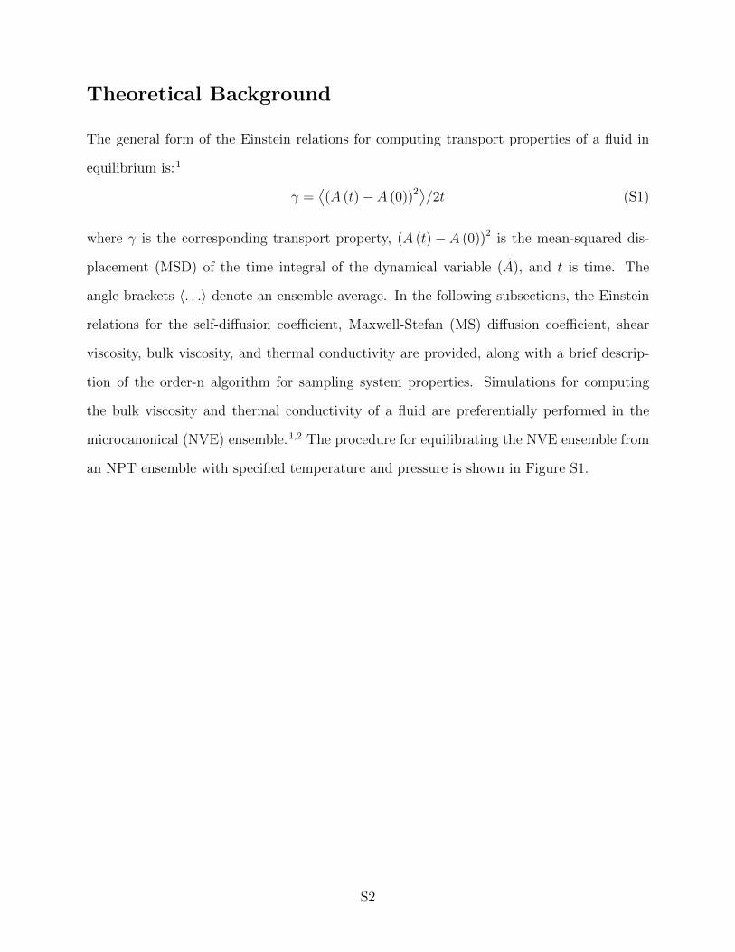
Theoretical Background

The general form of the Einstein relations for computing transport properties of a fluid in

equilibrium is:1

γ =⟨(A (t)− A (0))2⟩/2t (S1)

where γ is the corresponding transport property, (A (t)− A (0))2 is the mean-squared dis-

placement (MSD) of the time integral of the dynamical variable (A), and t is time. The

angle brackets 〈. . .〉 denote an ensemble average. In the following subsections, the Einstein

relations for the self-diffusion coefficient, Maxwell-Stefan (MS) diffusion coefficient, shear

viscosity, bulk viscosity, and thermal conductivity are provided, along with a brief descrip-

tion of the order-n algorithm for sampling system properties. Simulations for computing

the bulk viscosity and thermal conductivity of a fluid are preferentially performed in the

microcanonical (NVE) ensemble.1,2 The procedure for equilibrating the NVE ensemble from

an NPT ensemble with specified temperature and pressure is shown in Figure S1.

S2

Start

Equilibration

Production: sample volumeNPT ensemble

Equilibration

Production: sample total energy

Scale the simulation box to the average volume

Production:time-correlations

Transport properties

Finish

Change the total energy tothe average total energy

NVT ensemble

NVE ensemble

Input: T and P

Figure S1: Flowchart of the MD simulations for computing transport properties of a fluid.Each simulation starts with a simulation in the NPT ensemble, from which the averagevolume of the system is sampled. Then, the simulation box is scaled to this average volumewhich serves as the input for an equilibration run in the NVT ensemble. Consequently aproduction NVT run is performed from which the average energy of the system is sampled.This is used to scale the kinetic energy of the last configuration of the NVT run and is usedas input for a simulation in the NVE ensemble in which all properties are calculated.

S3

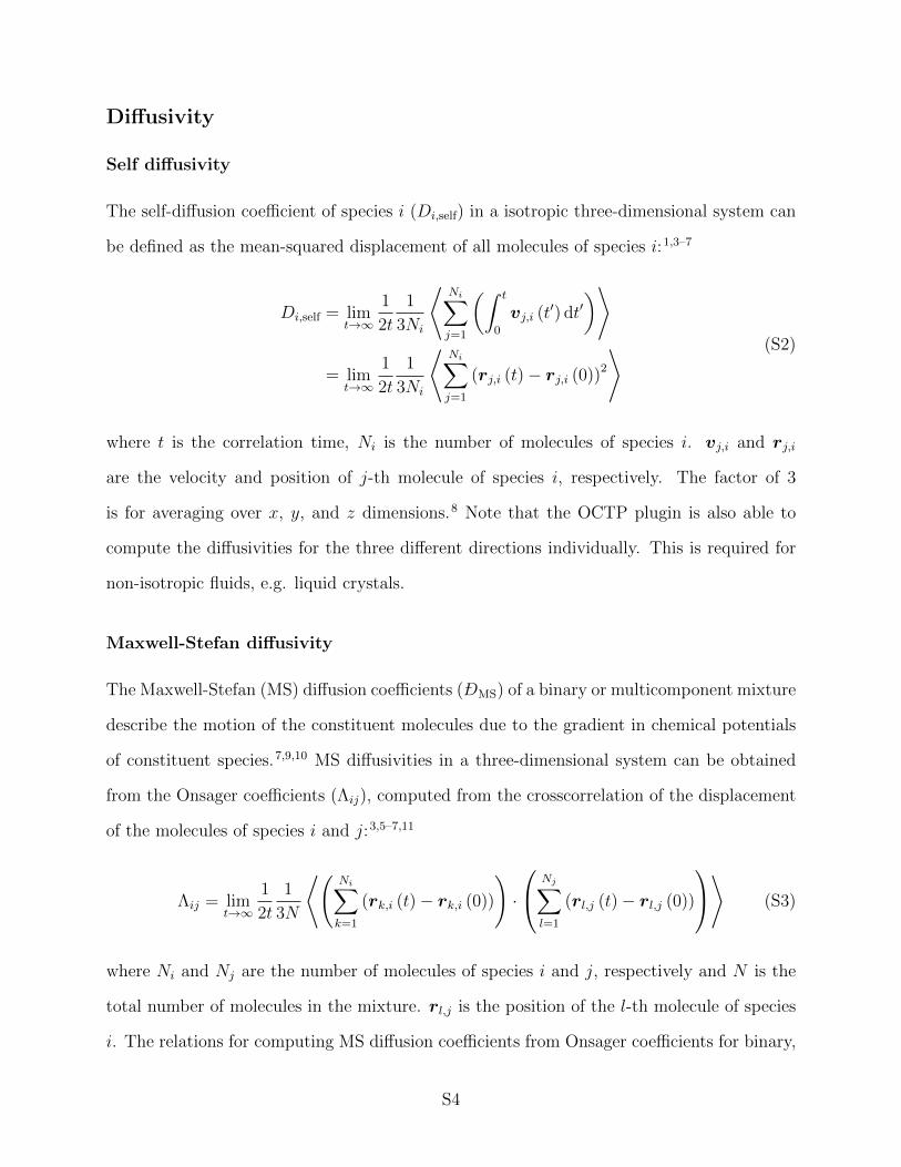
Diffusivity

Self diffusivity

The self-diffusion coefficient of species i (Di,self) in a isotropic three-dimensional system can

be defined as the mean-squared displacement of all molecules of species i:1,3–7

Di,self = limt→∞

1

2t

1

3Ni

⟨Ni∑j=1

(∫ t

0

vj,i (t′) dt′

)⟩

= limt→∞

1

2t

1

3Ni

⟨Ni∑j=1

(rj,i (t)− rj,i (0))2

⟩ (S2)

where t is the correlation time, Ni is the number of molecules of species i. vj,i and rj,i

are the velocity and position of j-th molecule of species i, respectively. The factor of 3

is for averaging over x, y, and z dimensions.8 Note that the OCTP plugin is also able to

compute the diffusivities for the three different directions individually. This is required for

non-isotropic fluids, e.g. liquid crystals.

Maxwell-Stefan diffusivity

The Maxwell-Stefan (MS) diffusion coefficients (DMS) of a binary or multicomponent mixture

describe the motion of the constituent molecules due to the gradient in chemical potentials

of constituent species.7,9,10 MS diffusivities in a three-dimensional system can be obtained

from the Onsager coefficients (Λij), computed from the crosscorrelation of the displacement

of the molecules of species i and j:3,5–7,11

Λij = limt→∞

1

2t

1

3N

⟨(Ni∑k=1

(rk,i (t)− rk,i (0))

)·

Nj∑l=1

(rl,j (t)− rl,j (0))

⟩ (S3)

where Ni and Nj are the number of molecules of species i and j, respectively and N is the

total number of molecules in the mixture. rl,j is the position of the l-th molecule of species

i. The relations for computing MS diffusion coefficients from Onsager coefficients for binary,

S4

ternary, and quaternary mixtures are listed in the articles by Krishna and van Baten,3 and

Liu et al.4,7,12,13 For a binary mixture with mole fractions of x1 and x2, a single MS diffusion

coefficient can be defined (D12,MS = D21,MS = DMS):3

DMS =x2

x1

Λ11 +x1

x2

Λ22 − 2Λ12 (S4)

Fick diffusivity

The Fick diffusion coefficient (DFick) describes the diffusion of molecules in a multicomponent

mixture as a result of the gradient in the concentration of constituent species.7,14 DFick and

DMS are related via the so-called thermodynamic factor (Γ). For a binary mixture, the

following algebraic relation holds:9

DFick = ΓDMS (S5)

where Γ for a multicomponent mixture is defined as:7,9,10,15

Γij = δij +∂ ln γi∂ lnxj

∣∣∣∣T,p,Σ

(S6)

in which γi is the activity coefficient of species i and δij is the Kronecker delta. The symbol Σ

indicates that the partial differentiation of lnγi with respect to mole fraction xj is carried out

at constant mole fraction of all other components except the n-th one, so that∑n

i=1 xi = 1

during the differentiation.15 There are different methods for computing the thermodynamic

factors such as using equations of state,3,16 the permuted Widom test particle insertion

method,17,18 and Kirkwood-Buff integrals.7,19–23 The last method has the advantage that

the required parameters are directly accessible from MD simulations. Analytic expressions

for Γij for various activity coefficient models are derived by Taylor and Kooijman.15

S5

Viscosity

Shear viscosity

The shear viscosity (η) is the resistance of a fluid to flow.24 η can be computed from the

time integral over the autocorrelation function of the off-diagonal components of the pressure

tensor (Pαβ,α 6=β):1,2,25,26

ηαβ = limt→∞

1

2t

V

kBT

⟨(∫ t

0

Pαβ (t′) dt′)2⟩

(S7)

where V is the volume of the system. The components of the pressure tensor are composed of

an ideal and a virial term. The first part is due to the total kinetic energy of particles and the

second is constructed from intra- and intermolecular interactions.1,27,28 In isotropic systems

(rotational invariance), the shear viscosities computed from any of the three off-diagonal

components of the pressure tensor (Pxy,Pxz, and Pyz) are equal. In isotropic systems, the

shear viscosity can also be computed from all components of the traceless pressure tensor

(P osαβ):25,26

η = limt→∞

1

10 · 2tV

kBT

⟨∑αβ

(∫ t

0

P osαβ (t′) dt′

)2⟩

(S8)

where26

P osαβ =

Pαβ + Pβα2

− δαβ

(1

3

∑k

Pkk

)(S9)

where δαβ is the Kronecker delta. The last term, i.e. one-third of the invariant trace of

the pressure tensor,29 equals the instantaneous kinetic pressure of the system (p). The

contribution of the diagonal components of the pressure tensor to the shear viscosity in

Equation (S8) is 4/3. Therefore, the contribution of all 9 components of the traceless pressure

tensor results in the factor 10 in the denominator of Equation (S8).

S6

Bulk viscosity

Bulk viscosity is a mysterious quantity - it is a transport coefficient, a property of the

continuum description of a flow - that points to the molecular world. It is related to the

equilibration of the energy of intramolecular degrees of freedom (rotations, vibrations) with

translational energy. For CO2, the bulk viscosity can be a thousand times larger than the

shear viscosity. The reason for such large bulk viscosity values lies in the fact that many

molecular collisions are needed to equilibrate the vibrational energy. Clearly, the value of

the bulk viscosity depends on how fast flow phenomena and energy transfer occur, and hence

the value of the bulk viscosity is frequency dependent. In Molecular Dynamics simulations,

the frequency dependent bulk viscocity can be computed from the van Hove correlation

function.30 At zero frequency, the bulk viscosity can be computed from the fluctuations in

kinetic pressure (δp):1

δp (t) = p (t)− 〈p〉 (S10)

where (p) is the instantaneous pressure and (〈p〉) the ensemble-averaged pressure. Accord-

ingly, the Einstein relation for the bulk viscosity is:1,31

ηb = limt→∞

1

2t

V

kBT

⟨(∫ t

0

δp (t′) dt′)2⟩

= limt→∞

1

2t

V

kBT

⟨(∫ t

0

(p (t′)− 〈p〉) dt′)2⟩

= limt→∞

1

2t

V

kBT

⟨(∫ t

0

p (t′) dt′ − 〈p〉 t)2⟩

= limt→∞

1

2t

V

kBT

⟨(∫ t

0

p (t′) dt

)2

− 2 〈p〉 t(∫ t

0

p (t′) dt

)+ (〈p〉 t)2

⟩(S11)

Thermal conductivity

The thermal conductivity (λ) describes the rate of heat conduction in a fluid as a result of

the temperature gradient in the system.24 λ can be computed from the components of the

S7

energy current/heat flux (Jα):1

λT = limt→∞

1

2t

V

kBT 2

⟨(∫ t

0

Jα (t′) dt′)2⟩

(S12)

The total heat flux consists of two parts: the kinetic heat flux (Jkinetic) and the potential

heat flux (Jpotential). The total heat flux is computed from:32

J = Jkinetic + Jpotential =1

2

Nt∑k=1

vk

[mv2

k +Nt∑

j=1,j 6=k

(φjk + rjk · f jk

)](S13)

where Nt is the total number of atoms in the system. vk is the velocity vector of atom i.

φjk, rjk, and f jk are the interaction potential, distance, and force between the two atoms

j and k. It is important to note here that Equation (S13) is valid for two-body interaction

potentials. For a detailed discussion on thermal conductivity computations in EMD the

reader is referred to the work of Kinaci et al.33

Order-n algorithm

The order-n algorithm samples time-correlation functions or MSDs at different sampling

frequencies.8,34 Several blocks (buffers) for each sampling frequency are created. For every

simulation timestep, it is examined if a buffer has to be updated based on the different

sampling frequencies. The oldest element within the buffer is used as the origin to compute

the time-correlation function/MSD. The computed quantity is added to an array which will

be used to obtain the ensemble-averaged MSD. The oldest element of the buffer is discarded

and all other elements are shifted one step to create a space for the newest system property

and this procedure continues. Details of the original order-n algorithm and the improved

algorithm which is used in this study can be found in the work of Dubbeldam et al.34

S8

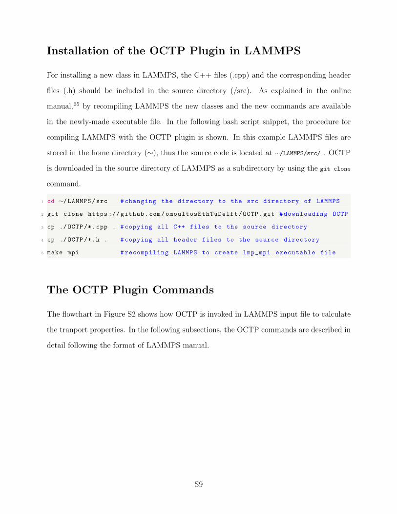
Installation of the OCTP Plugin in LAMMPS

For installing a new class in LAMMPS, the C++ files (.cpp) and the corresponding header

files (.h) should be included in the source directory (/src). As explained in the online

manual,35 by recompiling LAMMPS the new classes and the new commands are available

in the newly-made executable file. In the following bash script snippet, the procedure for

compiling LAMMPS with the OCTP plugin is shown. In this example LAMMPS files are

stored in the home directory (∼), thus the source code is located at ∼/LAMMPS/src/ . OCTP

is downloaded in the source directory of LAMMPS as a subdirectory by using the git clone

command.

1 cd ∼/LAMMPS/src #changing the directory to the src directory of LAMMPS

2 git clone https :// github.com/omoultosEthTuDelft/OCTP.git #downloading OCTP

3 cp ./OCTP /*. cpp . #copying all C++ files to the source directory

4 cp ./OCTP /*.h . #copying all header files to the source directory

5 make mpi #recompiling LAMMPS to create lmp_mpi executable file

The OCTP Plugin Commands

The flowchart in Figure S2 shows how OCTP is invoked in LAMMPS input file to calculate

the tranport properties. In the following subsections, the OCTP commands are described in

detail following the format of LAMMPS manual.

S9

Start

Integrate equations of motion

Update r, v, f at time t (t=t’+Δt)

LAMMPS OCTP

Input: positions (r), velcoities (v), and forces (f)

at time t’

Integrate dynamical variables

Sample MSD using the order-n algorithm

t+Δt < tmax

N

Finish

Update the timestep(t’=t)

Y

Invoke OCTPCompute system

properties (e.g., stress tensor)

Y

N

Output MSD files

Figure S2: Flowchart showing the use of OCTP in MD simulations with LAMMPS. Thesampling frequency specified for the OCTP plugin determines how frequently this plugin isinvoked. The system properties are calculated by using the relevant compute commands inLAMMPS. These properties are then integrated and sampled using the order-n algorithm.

S10

compute position command

Syntax

1 compute ID group -ID position

• ID, group-ID are described in compute command in LAMMPS35

• position = style name of this compute command

• no optional keyword

Example

1 compute c1 all position

Description

This command gathers the upwrapped positions, the atom IDs, and the group masks of all

atoms and passes this data as a global vector with size 5N , where N is the total number of

atoms in the system. This vector can be used in the command fix ordern to compute the

self-diffusion and Onsager coefficients. This command is developed based on the compute msd

command.35 This command should be used with the group-ID all.

S11

fix ordern command

Syntax

1 fix ID group -ID ordern style Nevery Nfreq value keyword values ...

• ID, group-ID are described in fix command in LAMMPS35

• ordern = style name of this fix command

• style = diffusivity, viscosity, or thermalconductivity

• Nevery = sample system properties every this timestep

• Nfreq = write output data files every this timestep

• value = c ID, global vector calculated by a compute with ID

• keyword values = optional arguments for fix ordern (see Table S1)

Table S1: Optional arguments for the new command fix ordern.

Argument Description Default

file name of the output file(s)diffusion (selfdiffusivity.dat and onsagercoefficient.dat)viscosity (viscosity.dat)thermal conductivity (thermalconductivity.dat)

format C-style string format to write data %gtitle text added to the top of output files -start start sampling after this number of steps 0Dxyz print x, y, z components of diffusivities if yes no (applicable only for the style diffusivity)

TCconvectiveprint convective portion of the thermal conductivity if yes

for more information see the manual35 for compute heat/fluxno (applicable only for the style thermalconductivity)

nb number of blocks for the order-n algorithm 10nbe number of block (buffer) elements for the order-n algorithm 10

Examples

1 fix 1 all ordern diffusivity 1000 100000 c_pos nb 10 nbe 20 title "

diffuison"

2 fix 2 all ordern viscosity 5 100000 c_P title viscosity start 10000

3 fix 3 all ordern thermalconductivity 5 100000 c_HF file thermcond.dat

S12

Description

This command computes the MSD of dynamic variables using the order-n algorithm. Three

styles can be defined: diffusivity, viscosity, and thermalconductivity. The corresponding

system properties for each style are sampled every Nevery timesteps. The ensemble-averaged

MSD is output to a file every Nfreq timesteps as a function of time. The system properties

required for these calculations are provided by a compute command.35 value specifies the ID

of this compute command (c ID). This compute should provide a global compute vector. This

fix does not return any values. It only outputs in data files the computed MSD as a function

of time. The corresponding transport properties can be calculated by linear regression at

timescales where MSD is a linear function of time. This fix command can be restarted. All

required data are automatically written to restart files generated by LAMMPS.

In this fix command, dynamical variables of the system are integrated prior to sampling

the MSD. For both viscosity and thermalconductivity styles, Simpson’s rule is used to in-

tegrate the corresponding dynamical variables. This means that the MSD is only available

at every 2×Nevery. Therefore, Nfreq should be a multiple of 2×Nevery. To improve the

accuracy of integration, it is suggested that Nevery should be between 1 and 10 timesteps

for viscosity and thermalconductivity. The sampling frequency when the style diffusivity is

used can be every hundreds to thousands timesteps. This is because the integration over the

positions has been already carried out at each timestep by the MD integration scheme.

The style diffusivity is used to compute MSDs for the calculation of self-diffusion and

Onsager coefficients. fix ordern accepts the global vector provided by the command compute

position. This compute command provides the positions of all atoms in the system along

with their atom IDs and group masks. To distinguish molecules of different species, an

atom type of each species should be specified via the group command.35 The only restriction

for using groups is that no atom should belong to two different groups at the same time.

If n groups are specified, this command outputs MSDs corresponding to n self-diffusion

coefficients and n(n + 1)/2 Onsager coefficients. Sample output files for self-diffusion and

S13

Onsager coefficients are shown in Tables S2 and S3, respectively. The MSDs reported in the

files are defined as:

MSDDi,self=

1

6

⟨Ni∑j=1

(rj,i (t)− rj,i (0))2

⟩(S14)

MSDΛij=

1

6

⟨(Ni∑k=1

(rk,i (t)− rk,i (0))

)·

Nj∑l=1

(rl,j (t)− rl,j (0))

⟩ (S15)

Note that the number of molecules of species i (Ni) and the total number of molecules

(N) (see Equations (S2) and (S3)) are not included in Equations (S14) and (S15). Thus, the

obtained MSDs must be divided by Ni and N , respectively. The reported MSDs in the output

files have already been divided by 6 (or 2 for the case of diffusion coefficients in directions

x, y, and z). The computed diffusion and Onsager coefficients from the provided MSDs

have units of distance2·time−1. For more information on the units available in LAMMPS,

the reader is referred to the manual.35 If the command units real, the units of computed

diffusion coefficients are in A2·fs−1.

S14

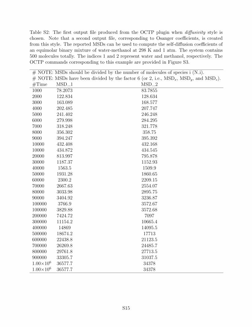
Table S2: The first output file produced from the OCTP plugin when diffusivity style ischosen. Note that a second output file, corresponding to Osanger coefficients, is createdfrom this style. The reported MSDs can be used to compute the self-diffusion coefficients ofan equimolar binary mixture of water-methanol at 298 K and 1 atm. The system contains500 molecules totally. The indices 1 and 2 represent water and methanol, respectively. TheOCTP commands corresponding to this example are provided in Figure S3.

# NOTE: MSDs should be divided by the number of molecules of species i (N i).# NOTE: MSDs have been divided by the factor 6 (or 2, i.e., MSDx, MSDy, and MSDz).#Time MSD 1 MSD 21000 78.2073 83.78552000 122.834 128.6343000 163.089 168.5774000 202.485 207.7475000 241.402 246.2486000 279.998 284.2957000 318.248 321.7788000 356.302 358.759000 394.247 395.39210000 432.408 432.16810000 434.872 434.54520000 813.997 795.87830000 1187.37 1152.9340000 1563.5 1509.950000 1931.28 1860.6560000 2300.2 2209.1570000 2667.63 2554.0780000 3033.98 2895.7590000 3404.92 3236.87100000 3766.9 3572.67100000 3829.88 3572.68200000 7424.72 7097300000 11154.2 10665.4400000 14869 14095.5500000 18674.2 17713600000 22438.8 21123.5700000 26269.8 24485.7800000 29761.8 27713.5900000 33305.7 31037.51.00×106 36577.7 343781.00×106 36577.7 34378

S15

Table S3: The second output file produced from the OCTP plugin when diffusivity style ischosen. The reported MSDs can be used to compute the Onsager coefficients of an equimolarbinary mixture of water-methanol at 298 K and 1 atm. The system contains 500 molecules.The indices 1 and 2 represent water and methanol, respectively. The OCTP commandscorresponding to this example are provided in Figure S3.

# NOTE: MSDs should be divided by the total number of molecules (N).# NOTE: MSDs have been divided by 6 (or 2, i.e., MSDx, MSDy, and MSDz).#Time MSD 1-1 MSD 1-2 MSD 2-21000 78.6612 -36.1723 28.45852000 122.458 -59.356 43.3063000 165.841 -82.108 57.78554000 215.892 -107.9207 73.19075000 260.7 -131.9022 87.64686000 304.815 -155.0308 101.1117000 352.803 -180.0117 114.6968000 398.088 -204.0983 128.6549000 445.89 -229.7967 143.19810000 493.083 -255.4383 157.43310000 491.533 -261.38 162.49520000 954.192 -535.2833 327.230000 1413.77 -794.2267 472.33840000 1883.75 -1051.605 615.54350000 2324.05 -1294.4333 748.72360000 2678.15 -1505.21 872.82770000 3127.52 -1761.4667 1021.4580000 3650.48 -2062.1833 1194.9290000 4167.9 -2346.8167 1349.84100000 4646.98 -2611.1 1498.82100000 4605.6 -2593.9667 1500.61200000 8312.03 -4613.3667 2603.97300000 9677.52 -5367.6333 3015.1400000 9937.93 -5435.9 3013.63500000 14731.1 -8184.1667 4596.8600000 20837 -11591.8 6468.67700000 23588.2 -13261.9333 7484.8800000 20415.5 -11528.3667 6536.53900000 19109.2 -10913.0667 6257.531.00×106 11490.2 -6267.15 3422.11.00×106 11490.2 -6267.15 3422.1

S16

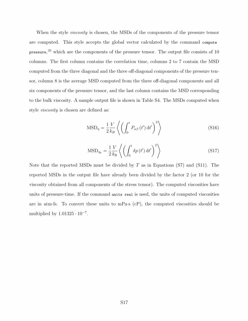
When the style viscosity is chosen, the MSDs of the components of the pressure tensor

are computed. This style accepts the global vector calculated by the command compute

pressure,35 which are the components of the pressure tensor. The output file consists of 10

columns. The first column contains the correlation time, columns 2 to 7 contain the MSD

computed from the three diagonal and the three off-diagonal components of the pressure ten-

sor, column 8 is the average MSD computed from the three off-diagonal components and all

six components of the pressure tensor, and the last column contains the MSD corresponding

to the bulk viscosity. A sample output file is shown in Table S4. The MSDs computed when

style viscosity is chosen are defined as:

MSDη =1

2

V

kB

⟨(∫ t

0

Pαβ (t′) dt′)2⟩

(S16)

MSDηb =1

2

V

kB

⟨(∫ t

0

δp (t′) dt′)2⟩

(S17)

Note that the reported MSDs must be divided by T as in Equations (S7) and (S11). The

reported MSDs in the output file have already been divided by the factor 2 (or 10 for the

viscosity obtained from all components of the stress tensor). The computed viscosities have

units of pressure·time. If the command units real is used, the units of computed viscosities

are in atm·fs. To convert these units to mPa·s (cP), the computed viscosities should be

multiplied by 1.01325 · 10−7.

S17

Table S4: Output file obtained when the viscosity style is chosen. These MSDs can beused to compute the shear and bulk viscosities of an equimolar mixture of water-methanolat 298 K and 1 atm. The system contains 500 molecules. The MSDs of columns 2 to 4and 5 to 7 are computed from the diagonal and off-diagonal components of the pressuretensor, respectively. Columns 8 and 9 are the average MSDs from the off-diagonal and allcomponents of the pressure tensor, respectively. Column 10 contains the MSDs computedfrom the fluctuation of the kinetic pressure to calculate the bulk viscosity. The OCTPcommands corresponding to this example are provided in Figure S3.

#NOTE: MSDs should be divided by the temperature.#NOTE: MSDs have been divided by 2 or 10 (i.e., the viscosity computed from all components).#Time MSD xx MSD yy MSD zz MSD xy MSD xz MSD yz MSD off MSD all MSD bulkvisc10 1.02×109 1.01×109 1.01×109 1.02×109 1.02×109 1.04×109 1.03×109 1.02×109 1.15×109

20 3.26×109 3.22×109 3.21×109 3.28×109 3.26×109 3.31×109 3.29×109 3.26×109 4.28×109

30 6.77×109 6.68×109 6.67×109 6.82×109 6.78×109 6.89×109 6.83×109 6.78×109 9.22×109

40 1.10×1010 1.09×1010 1.09×1010 1.12×1010 1.11×1010 1.13×1010 1.12×1010 1.11×1010 1.56×1010

50 1.57×1010 1.55×1010 1.54×1010 1.59×1010 1.58×1010 1.60×1010 1.59×1010 1.58×1010 2.32×1010

60 2.09×1010 2.06×1010 2.05×1010 2.12×1010 2.10×1010 2.14×1010 2.12×1010 2.10×1010 3.19×1010

70 2.61×1010 2.56×1010 2.55×1010 2.65×1010 2.62×1010 2.67×1010 2.65×1010 2.62×1010 4.12×1010

80 3.16×1010 3.10×1010 3.08×1010 3.21×1010 3.17×1010 3.24×1010 3.21×1010 3.17×1010 5.13×1010

90 3.71×1010 3.64×1010 3.62×1010 3.77×1010 3.73×1010 3.82×1010 3.77×1010 3.73×1010 6.18×1010

100 4.27×1010 4.20×1010 4.16×1010 4.36×1010 4.30×1010 4.41×1010 4.36×1010 4.30×1010 7.26×1010

100 4.28×1010 4.17×1010 4.14×1010 4.36×1010 4.30×1010 4.40×1010 4.35×1010 4.29×1010 7.28×1010

200 1.11×1011 1.09×1011 1.08×1011 1.13×1011 1.12×1011 1.17×1011 1.14×1011 1.12×1011 1.88×1011

300 1.99×1011 1.94×1011 1.92×1011 2.02×1011 2.01×1011 2.10×1011 2.04×1011 2.01×1011 3.14×1011

400 3.02×1011 2.93×1011 2.89×1011 3.07×1011 3.06×1011 3.20×1011 3.11×1011 3.04×1011 4.58×1011

500 4.17×1011 4.02×1011 3.97×1011 4.24×1011 4.23×1011 4.44×1011 4.30×1011 4.21×1011 6.19×1011

600 5.44×1011 5.20×1011 5.16×1011 5.53×1011 5.52×1011 5.82×1011 5.62×1011 5.48×1011 7.94×1011

700 6.82×1011 6.46×1011 6.45×1011 6.93×1011 6.91×1011 7.31×1011 7.05×1011 6.86×1011 9.83×1011

800 8.29×1011 7.81×1011 7.83×1011 8.41×1011 8.39×1011 8.90×1011 8.57×1011 8.33×1011 1.19×1012

900 9.86×1011 9.22×1011 9.30×1011 9.99×1011 9.95×1011 1.06×1012 1.02×1012 9.89×1011 1.40×1012

1000 1.15×1012 1.07×1012 1.08×1012 1.17×1012 1.16×1012 1.24×1012 1.19×1012 1.15×1012 1.63×1012

1000 1.16×1012 1.08×1012 1.09×1012 1.21×1012 1.18×1012 1.19×1012 1.19×1012 1.16×1012 1.65×1012

2000 3.23×1012 2.81×1012 2.94×1012 3.20×1012 3.13×1012 3.34×1012 3.22×1012 3.13×1012 4.35×1012

3000 5.75×1012 4.78×1012 5.18×1012 5.57×1012 5.31×1012 6.04×1012 5.64×1012 5.48×1012 7.55×1012

4000 8.52×1012 6.88×1012 7.65×1012 8.15×1012 7.50×1012 9.07×1012 8.24×1012 8.02×1012 1.10×1013

5000 1.15×1013 9.19×1012 1.02×1013 1.08×1013 9.60×1012 1.22×1013 1.09×1013 1.07×1013 1.47×1013

6000 1.47×1013 1.17×1013 1.29×1013 1.34×1013 1.18×1013 1.55×1013 1.36×1013 1.34×1013 1.88×1013

7000 1.80×1013 1.43×1013 1.55×1013 1.61×1013 1.39×1013 1.88×1013 1.63×1013 1.61×1013 2.31×1013

8000 2.13×1013 1.70×1013 1.80×1013 1.89×1013 1.61×1013 2.22×1013 1.91×1013 1.89×1013 2.76×1013

9000 2.46×1013 1.98×1013 2.06×1013 2.17×1013 1.85×1013 2.55×1013 2.19×1013 2.18×1013 3.24×1013

10000 2.81×1013 2.27×1013 2.31×1013 2.47×1013 2.08×1013 2.88×1013 2.48×1013 2.47×1013 3.71×1013

10000 3.03×1013 2.27×1013 2.49×1013 2.44×1013 2.03×1013 3.00×1013 2.49×1013 2.53×1013 3.75×1013

20000 6.70×1013 5.02×1013 5.21×1013 5.91×1013 4.22×1013 6.31×1013 5.48×1013 5.55×1013 8.77×1013

30000 1.01×1014 7.99×1013 8.30×1013 9.46×1013 6.23×1013 9.84×1013 8.51×1013 8.63×1013 1.42×1014

40000 1.46×1014 1.19×1014 1.27×1014 1.28×1014 8.78×1013 1.17×1014 1.11×1014 1.19×1014 1.93×1014

50000 1.90×1014 1.55×1014 1.71×1014 1.63×1014 1.12×1014 1.24×1014 1.33×1014 1.49×1014 2.41×1014

60000 2.34×1014 1.99×1014 2.22×1014 1.88×1014 1.38×1014 1.35×1014 1.54×1014 1.80×1014 2.91×1014

70000 2.64×1014 2.38×1014 2.72×1014 2.09×1014 1.58×1014 1.52×1014 1.73×1014 2.07×1014 3.37×1014

80000 2.95×1014 2.71×1014 3.25×1014 2.26×1014 1.76×1014 1.75×1014 1.92×1014 2.34×1014 3.72×1014

90000 3.15×1014 3.04×1014 3.81×1014 2.33×1014 1.98×1014 2.01×1014 2.11×1014 2.60×1014 3.91×1014

100000 3.33×1014 3.43×1014 4.37×1014 2.42×1014 2.23×1014 2.30×1014 2.32×1014 2.87×1014 4.00×1014

100000 5.52×1014 4.58×1014 6.27×1014 3.55×1014 1.28×1014 2.15×1014 2.33×1014 3.58×1014 3.12×1014

200000 7.13×1014 5.80×1014 1.37×1015 3.39×1014 3.96×1014 6.15×1014 4.50×1014 6.25×1014 1.83×1014

300000 7.61×1014 7.07×1014 1.79×1015 6.31×1014 8.20×1014 9.05×1014 7.85×1014 9.06×1014 3.97×1014

400000 1.29×1015 1.27×1015 2.51×1015 8.63×1014 1.30×1015 1.34×1015 1.17×1015 1.38×1015 3.72×1014

500000 1.24×1015 1.72×1015 3.41×1015 1.18×1015 1.82×1015 2.06×1015 1.69×1015 1.86×1015 5.20×1014

600000 8.60×1014 2.09×1015 4.14×1015 1.64×1015 2.59×1015 2.93×1015 2.38×1015 2.38×1015 3.87×1014

700000 9.70×1014 3.24×1015 4.46×1015 1.96×1015 3.21×1015 3.79×1015 2.99×1015 2.95×1015 3.24×1014

800000 5.66×1014 4.30×1015 4.56×1015 2.77×1015 4.02×1015 4.48×1015 3.76×1015 3.51×1015 3.34×1014

900000 1.03×1014 4.24×1015 3.55×1015 3.23×1015 4.95×1015 6.52×1015 4.90×1015 3.99×1015 3.30×1014

1.00×106 2.38×1015 8.29×1015 1.79×1015 3.54×1015 6.41×1015 7.82×1015 5.92×1015 5.21×1015 7.59×108

1.00×106 2.38×1015 8.29×1015 1.79×1015 3.54×1015 6.41×1015 7.82×1015 5.92×1015 5.21×1015 7.59×108

S18

The style thermalconductivity is used to compute MSDs of the energy current/heat flux,

from which the thermal conductivity can be calculated. This style accepts the global vector

calculated by compute heat/flux.35 The output file (see an example in Table S5) reports the

MSD computed from the three components of the heat flux (x, y, and z), followed by the

average of all components as a function of time. The MSDs computed when thermalconduc-

tivity style is chosen is defined as:

MSDλT =1

2

V

kB

⟨(∫ t

0

Jα (t′) dt′)2⟩

(S18)

Note that the reported MSDs must be divided by T 2 as in Equation (S12). The MSDs

reported in the output file have already been divided by 2. The computed thermal conduc-

tivities have units of energy·distance−1·temperature−1·time−1. If the command units real is

used, the units of computed thermal conductivities are kcal·mol−1·A−1·K−1·fs−1. To convert

these units to W·m−1·K−1, the computed properties should be multiplied by 6.9477 · 104.

S19

Table S5: Output file obtained when the thermalconductivity style is chosen. These MSDscan be used to compute the thermal conductivity of an equimolar mixture of water-methanolat 298 K and 1 atm. The system contains 500 molecules. The MSDs reported in columns 2to 4 are calculated from the components of the heat flux vector. The average from the threecomponents is listed in column 5. The OCTP commands corresponding to this example areprovided in Figure S3.

# NOTE: MSDs should be divided by (temperatureˆ2).# NOTE: MSDs have been divided by 2.#Time MSD x MSD y MSD z MSD all10 6.14796 6.04591 6.05702 6.0836320 16.9439 16.6303 16.696 16.756730 25.7431 25.2557 25.4648 25.487840 30.798 30.2201 30.5988 30.53950 34.8567 34.1091 34.6857 34.550560 41.6606 40.5192 41.4167 41.198970 50.3229 48.5958 49.9849 49.634680 59.4713 57.1289 59.1014 58.567290 67.689 64.8516 67.2842 66.6083100 74.974 71.7629 74.5068 73.7479100 75.3937 71.9785 73.9582 73.7768200 148.499 140.433 147.295 145.409300 216.157 204.382 211.053 210.531400 279.572 263.181 268.949 270.567500 340.476 321.524 324.151 328.717600 396.735 376.955 379.506 384.399700 452.05 430.876 433.366 438.764800 506.239 488.334 481.969 492.181900 558.893 546.774 530.8 545.4891000 610.095 604.337 579.614 598.0151000 612.992 591.925 555.888 586.9352000 1111.81 1118.97 989.736 1073.513000 1595.06 1629.51 1440.87 1555.154000 2105.55 2138.1 1834.11 2025.925000 2626.31 2591.98 2235.56 2484.626000 3055.28 3022.96 2663.39 2913.887000 3535.53 3432.9 3093.31 3353.918000 4006.1 3822.18 3519.3 3782.529000 4460.53 4237.4 3945.58 4214.510000 4945.63 4674.69 4402.65 4674.3210000 5281.72 4627.21 4494.12 4801.0220000 10046.9 9352.87 10196.5 9865.430000 14362.6 13602 16625.1 14863.240000 17830.9 17715.1 23617.1 1972150000 20345.1 23228.6 31729.8 25101.260000 23638.3 28144 40613.2 30798.570000 25649.1 33091.1 47831.1 35523.880000 27750.3 37172.7 52676.2 39199.790000 31189.6 43184.8 58610.2 44328.2100000 34153.9 47337.5 64462.9 48651.4100000 33917.8 39154.2 76568.8 49880.3200000 71830.1 66682.6 150588 96367300000 89178.9 109313 262698 153730400000 97787.4 130251 425249 217762500000 82688.3 198854 664211 315251600000 102158 206431 835281 381290700000 149280 246085 990271 461879800000 250730 364304 957791 524275900000 486497 440610 975287 6341311.00×106 490899 448789 1.29×106 7447121.00×106 490899 448789 1.29×106 744712

S20

A list of available optional arguments for fix ordern is presented in Table S1. The keyword

file followed by one string (for style viscosity and thermalconductivity) or two strings (for

style diffusivity) defines the name(s) of the output file(s). The keyword format followed by a

string containing a C-style string format defines the precision of the data written in data files.

The keyword title followed by a string provides the possibility to add an optional text to the

header of the output files. The keyword start specifies for how many timesteps the sampling

is postponed (i.e., the time at which the sampling starts). The keyword Dxyz followed

by either yes/no enables/disables the functionality to write the x, y, and z components

of self-diffusivities and Onsager coefficients in the output files, respectively. The keyword

TCconductive followed by either yes/no enables/disables the functionality to write the x, y,

and z components as well as the average of the convective portion of the thermal conductivity

in the output file. For more information, the reader is referred to the LAMMPS manual for

the command compute heat/flux. The keywords nb and nbe specify the number of blocks and

the number of elements for each block. The default value for both nb and nbe is 10. This

means that fix ordern can sample MSD for timescales ranging from 1×Nevery to 1010×Nevery

timesteps.

S21

compute rdf/ext command

Syntax

1 compute ID group -ID rdf/ext keyword values

• ID, group-ID are described in compute command in LAMMPS35

• rdf/ext = style name of this compute command

• keyword = Nbin, Nfreq, file

Example

1 compute c2 all rdf/ext Nbin 2000 Nwrite 100 file rdf.dat

2 fix fc2 all ave/time 1 1 1000 c_c2

Description

This command computes the radial distribution function (RDF; gij) for all pairs of atom

types specified by the command group.35 This command should be used with the group-ID

all. For a system consisting of n groups, n(n+ 1)/2 RDFs can be computed. The computed

RDFs are reported in histogram form. The number of bins can be specified via the keyword

Nbin. The default number of bins is 1000. RDFs computed in MD simulations depend on the

system-size. In compute rdf/ext the finite-size RDFs are corrected according to the work of

van der Vegt and co-workers.36,37 For each pair of groups, both the finite-size and corrected

RDF histograms are output. The command fix ave/time35 is used to invoke compute rdf/ext.

In the example, fix ave/time is invoked with a sampling rate of 1000 timesteps. The keyword

Nwrite, followed by a number, is used to specify the writing frequency in the output file. The

default value for Nwrite is 1000. The name of the output file can be modified by the keyword

file. compute rdf is developed based on the compute msd and compute rdf commands.35 compute

rdf/ext has the following two advantages over compute rdf: (1) it computes RDFs beyond

the cutoff radius; and (2) corrects RDFs for the finite-size effects.

S22

Sample script

A sample script of the LAMMPS input file using the OCTP commands is shown in Fig-

ure S3 for the calculation of diffusion coefficients, viscosities, and thermal conductivities of

an equimolar water-methanol mixture.

At lines 1-5, the computation of MSDs related to the diffusion coefficients is specified by

using the style diffusivity. For the binary water-methanol mixture, two groups are defined at

lines 2 and 3 to tag all oxygen atoms of water (i.e., type 5) and all oxygen atoms of methanol

(i.e., type 4) with the corresponding group IDs of 1 and 2. These IDs are used in the code to

identify that the system is binary and, thus compute two MSDs (one for each component)

and three Onsager coefficients. At line 4, the command compute position is used to obtain

the position of all atoms in the simulation box, which is needed as an input for fix ordern

(line 5). The sampling frequency of positions is specified by the variable ${Ndiff}, while the

1 # computing diffusion coefficients

2 group 1 type 5 # The Oxygen of the water

3 group 2 type 4 # The Oxygen of the methanol

4 compute positions all position

5 fix fix1 all ordern diffusivity ${Ndiff} ${Nwrite} c_positions

6

7 # computing viscosity and average pressure

8 compute T all temp

9 compute P all pressure T

10 fix fix2 all ordern viscosity ${Nvis} ${Nwrite} c_P

11

12 # computing thermal conductivity

13 compute KE all ke/atom

14 compute PE all pe/atom

15 compute ST all stress/atom NULL virial

16 compute heatflux all heat/flux KE PE ST

17 fix fix3 all ordern thermalconductivity ${Ntherm} ${Nwrite} c_heatflux

Figure S3: Sample script for computing transport properties in LAMMPS using the OCTPplugin. The MSDs related to diffusivities, viscosities, and thermal conductivities are com-puted using the fix ordern command. The variables ${Nvis}, ${Ntherm}, and ${Ndiff}specify the sampling frequency of system properties, while output data are written every${Nwrite} timesteps. The required system properties for fix ordern are provided by thecommands compute position , compute pressure,35 and compute heat/flux.35 In this script, nooptional arguments are used.

S23

output frequency in data files is specified by the variable ${Nwrite}.

At lines 7-10 and 12-16, the OCTP commands for computing MSDs related to the vis-

cosities and thermal conductivities are specified, respectively. The corresponding compute

commands are compute pressure (line 9) and compute heat/flux (line 16). These two com-

mands require the instantaneous temperature of the system (line 8), and per-atom kinetic

energy (line 13), potential energy (line 14), and pressure tensor (line 15), respectively.

S24

Finite-size Effects of Transport Properties of a Lennard-

Jones Fluid Close to the Critical Point

OCTP is used to investigate the finite-size effects of transport properties of a Lennard-Jones

(LJ) fluid. The LJ size (σ = 1) and energy (ε = 1) parameters, along with the mass = 1 are

in reduced units.1 To ensure the smooth integration in Equation (S17) the shifted-force 12-6

LJ potential with a cutoff radius (rc) of 2.5σ is used:1

ULJ,shifted-force (rij) =

ULJ (rij)− ULJ (rc)− (rij − rc)

(dULJ

drij

)rij=rc

r ≤ rc

0 r > rc

(S19)

where rij is the distance between two particles i and j.38 The temperature (T ) and density

(ρ) of MD simulations are 1.00 and 0.325, respectively, which is close to the critical point

(Tc = 0.937 and ρc = 0.320).39 MD simulations were performed in the NVE ensemble

according to the procedure shown in Figure S1. Four system sizes were considered: 500,

1000, 2000, and 4000 LJ particles. At least 5 independent simulations were performed for

each system size to compute 95% confidence intervals.

The finite-size transport properties are shown in Figure S4. These properties are: (panel

a) the self-diffusivity, (panel b) the shear viscosity, (panel c) bulk viscosity, and (panel d)

thermal conductivity. Except for shear viscosity, all transport properties show a strong

system-size dependency. In agreement with our recent work,40 the analytic correction pro-

posed by Yeh and Hummer41,42 does not hold for finite-size effects of self-diffusivities close

to the critical point. Bulk viscosity shows the maximum finite-size effect, for which the value

in the thermodynamic limit is almost three times the value computed from a system of 500

LJ particles.

S25

0.4

0.42

0.44

0.46

0.48

0.5

0 0.02 0.04 0.06 0.08 0.1

(a)D

self

/ [ σ

ε1/

2 m

-1/2

]

L-1 / [σ-1]

0.2

0.22

0.24

0.26

0.28

0.3

0 0.02 0.04 0.06 0.08 0.1

(b)

ηsh

ear /

[ σ

2 m

-1/2

ε-1

/2]

L-1 / [σ-1]

0

0.4

0.8

1.2

1.6

2

0 0.02 0.04 0.06 0.08 0.1

(c)

ηbu

lk /

[ σ2

m-1

/2 ε

-1/2

]

L-1 / [σ-1]

1.4

1.5

1.6

1.7

1.8

1.9

0 0.02 0.04 0.06 0.08 0.1

(d)

λ /

[ ε1/

2 σ

-2 m

-1/2

]

L-1 / [σ-1]

Figure S4: (a) Self-diffusion coefficient, (b) shear viscosity, (c) bulk viscosity, and (d) thermalconductivity of a LJ fluid close to the critical point as a function of the simulation box length(L). Blue circles are the computed finite-size transport properties. The dashed lines indicateextrapolation to the thermodynamic limit, and the solid lines show the values of the transportproperties at the thermodynamic limit. Error bars correspond to 95% confidence intervals.Red squares are the corrected self-diffusivities using the analytic relation proposed by Yehand Hummer.41 Properties are reported in reduced units1 with σ, ε, and mass equal to 1.The shifted-force potential at a cutoff radius of 2.5σ is used. The critical temperature anddensity of this LJ fluid is 0.937 and 0.320, respectively.39 The temperature and density ofthe system are 1.00 and 0.325, respectively.

S26

Details of Water-Methanol Mixture Simulations

MD simulations were performed to compute the self-diffusivities, Maxwell-Stefan diffu-

sion coefficients, shear viscosity, and thermal conductivity of a water-methanol mixture

(xmethanol = 0.5) at 298 K and 1 atm. To investigate the computational requirements

and scaling behaviour of the OCTP plugin, 6 system sizes of 250, 500, 1000, 2000, 4000,

and 8000 molecules were considered. The SPC/E water model43 and the TraPPE-UA force

field44 for methanol are used. Non-bonded interactions are truncated at a cutoff radius of

10 A. Analytic tail corrections are included for the calculation of energy and pressure. The

Lorentz-Berthelot mixing rules are used for the interactions of unlike atoms.1 Long-range

electrostatic interactions are considered using the particle-particle particle-mesh (PPPM)

method with a relative precision of 10−6.1,35 All simulations are performed according to

the procedure shown in Figure S1. The length of the production runs is 1 ns. Dynamical

variables are sampled every 1000, 5, and 5 timesteps, for diffusion coefficients, viscosities,

and thermal conductivity, respectively. The computed MSDs for Onsager coefficients, shear

viscosity, and thermal conductivity are shown in Figure S5. The MS diffusion coefficients

are computed from the Onsager coefficients (see Equation (S4)). The transport coefficients

are obtained by linear regression at timescales where the slope of MSD is equal to 1 in the

log-log plots.1,34 As shown in Figure S5, at large timescales (t > 100 ps), the small number

of samples leads to scattered MSDs. The observed jumps at 10 ps and 100 ps are due to the

different number of samples at a correlation time in two different blocks.

All input files for LAMMPS to simulate the water-methanol system are provided as a

separate Supporting Information file.

S27

0.1

1

10

100

1 10 100 1000

(a)M

SD

Ons

ager

coe

ffici

ent /

[Å2 ]

t / [ps]

1

10

100

1000

1 10 100 1000

(b)

MS

Dsh

ear v

isco

sity

/ [c

P.p

s]

t / [ps]

1

10

100

1000

1 10 100 1000

(c)

MS

Dt.

cond

uctiv

ity /

[W.m

-1.K

-1.p

s]

t / [ps]

Figure S5: Computed MSDs for (a) Onsager coefficients (blue line: Λwater-water, red line:Λmethanol-methanol, and green line: -Λwater-methanol), (b) shear viscosity, and (c) thermal con-ductivity for a water-methanol mixture (xmethanol = 0.5). Solid lines are computed from theOCTP plugin, while crosses represent the MSDs obtained by postprocessing trajectory filesusing the order-n algorithm. The dashed lines represent the slope of 1 in these log-log plots.

S28

References

(1) Allen, M. P.; Tildesley, D. J. Computer Simulation of Liquids, 2nd ed.; Oxford Univer-

sity Press: Croydon, 2017.

(2) Zwanzig, R. Time-Correlation Functions and Transport Coefficients in Statistical Me-

chanics. Annu. Rev. Phys. Chem. 1965, 16, 67–102.

(3) Krishna, R.; van Baten, J. M. The Darken Relation for Multicomponent Diffusion in

Liquid Mixtures of Linear Alkanes: An Investigation Using Molecular Dynamics (MD)

Simulations. Ind. Eng. Chem. Res. 2005, 44, 6939–6947.

(4) Liu, X.; Vlugt, T. J. H.; Bardow, A. Maxwell-Stefan Diffusivities in Liquid Mixtures:

Using Molecular Fynamics for Testing Model Predictions. Fluid Phase Equilib. 2011,

301, 110–117.

(5) Liu, X.; Schnell, S. K.; Simon, J.-M.; Bedeaux, D.; Kjelstrup, S.; Bardow, A.; Vlugt, T.

J. H. Fick Diffusion Coefficients of Liquid Mixtures Directly Obtained From Equilibrium

Molecular Dynamics. J. Phys. Chem. B 2011, 115, 12921–12929.

(6) Liu, X.; Vlugt, T. J. H.; Bardow, A. Maxwell-Stefan Diffusivities in Binary Mixtures

of Ionic Liquids with Dimethyl Sulfoxide (DMSO) and H2O. J. Phys. Chem. B 2011,

115, 8506–8517.

(7) Liu, X.; Schnell, S. K.; Simon, J.-M.; Kruger, P.; Bedeaux, D.; Kjelstrup, S.; Bar-

dow, A.; Vlugt, T. J. H. Diffusion Coefficients from Molecular Dynamics Simulations

in Binary and Ternary Mixtures. Int. J. Thermophys. 2013, 34, 1169–1196.

(8) Frenkel, D.; Smit, B. Understanding Molecular Simulation: From Algorithms to Appli-

cations, 2nd ed.; Academic Press: London, 2002.

(9) Taylor, R.; Krishna, R. Multicomponent Mass Transfer ; John Wiley & Sons: New York,

1993.

S29

(10) Krishna, R.; van Baten, J. M. Describing Diffusion in Fluid Mixtures at Elevated

Pressures by Combining the Maxwell-Stefan Formulation with an Equation of State.

Chem. Eng. Sci. 2016, 153, 174–187.

(11) Liu, X.; Bardow, A.; Vlugt, T. J. H. Multicomponent Maxwell-Stefan Diffusivities at

Infinite Dilution. Ind. Eng. Chem. Res. 2011, 50, 4776–4782.

(12) Liu, X.; Vlugt, T. J. H.; Bardow, A. Predictive Darken Equation for Maxwell-Stefan

Diffusivities in Multicomponent Mixtures. Ind. Eng. Chem. Res. 2011, 50, 10350–

10358.

(13) Liu, H.; Maginn, E. A Molecular Dynamics Investigation of the Struc-

tural and Dynamic Properties of the Ionic Liquid 1-n-Butyl-3-methylimidazolium

Bis(Trifluoromethanesulfonyl)imide. J. Chem. Phys. 2011, 135, 124507.

(14) Keffer, D. J.; Gao, C. Y.; Edwards, B. J. On the Relationship between Fickian Diffusiv-

ities at the Continuum and Molecular Levels. J. Phys. Chem. B 2005, 109, 5279–5288.

(15) Taylor, R.; Kooijman, H. A. Composition Derivatives of Activity Coefficient Models

(For the Estimation of Thermodynamic Factors in Diffusion). Chem. Eng. Commun.

1991, 102, 87–106.

(16) Krishna, R.; Wesselingh, J. The Maxwell-Stefan Approach to Mass Transfer. Chem.

Eng. Sci. 1997, 52, 861–911.

(17) Balaji, S. P.; Schnell, S. K.; McGarrity, E. S.; Vlugt, T. J. H. A Direct Method for

Calculating Thermodynamic Factors for Liquid Mixtures Using the Permuted Widom

Test Particle Insertion Method. Mol. Phys. 2013, 111, 287–296.

(18) Balaji, S. P.; Schnell, S. K.; Vlugt, T. J. H. Calculating Thermodynamic Factors of

Ternary and Multicomponent Mixtures Using the Permuted Widom Test Particle in-

sertion Method. Theor. Chem. Acc. 2013, 132, 1333.

S30

(19) Zhou, Y.; Miller, G. H. Green-Kubo Formulas for Mutual Diffusion Coefficients in

Multicomponent Systems. J. Phys. Chem. 1996, 100, 5516–5524.

(20) Ben-Naim, A. Molecular Theory of Solutions ; Oxford University Press: Oxford, 2006.

(21) Kruger, P.; Schnell, S. K.; Bedeaux, D.; Kjelstrup, S.; Vlugt, T. J. H.; Simon, J.-M.

Kirkwood-Buff Integrals for Finite Volumes. J. Phys. Chem. Lett. 2013, 4, 235–238.

(22) Kruger, P.; Vlugt, T. J. H. Size and Shape Dependence of Finite-volume Kirkwood-Buff

Integrals. Phys. Rev. E 2018, 97, 051301.

(23) Dawass, N.; Kruger, P.; Schnell, S. K.; Simon, J.-M.; Vlugt, T. J. H. Kirkwood-Buff

Integrals from Molecular Simulation. Fluid Phase Equilib. 2019, 486, 21–36.

(24) Poling, B. E.; Prausnitz, J. M.; O’Connel, J. P. The Properties of Gases and Liquids,

5th ed.; McGraw-Hill: Singapore, 2001.

(25) Mondello, M.; Grest, G. S. Viscosity Calculations of n-Alkanes by Equilibrium Molec-

ular Dynamics. J. Chem. Phys. 1997, 106, 9327.

(26) Tenney, C. M.; Maginn, E. J. Limitations and Recommendations for the Calculation

of Shear Viscosity using Reverse Nonequilibrium Molecular Dynamics. J. Chem. Phys.

2010, 132, 014103.

(27) Heyes, D. M. Pressure Tensor of Partial-Charge and Point-Dipole Lattices with Bulk

and Surface Geometries. Phys. Rev. B 1994, 49, 755–764.

(28) Thompson, A. P.; Plimpton, S. J.; Mattson, W. General Formulation of Pressure and

Stress Tensor for Arbitrary Many-Body Interaction Potentials Under periodic Boundary

Conditions. J. Chem. Phys. 2009, 131, 154107.

(29) Meador, W. E.; Miner, G. A.; Townsend, L. W. Bulk viscosity as a relaxation parameter:

Fact or fiction? Phys. Fluids 1996, 8, 258–261.

S31

(30) Evans, D. J.; Morriss, G. Statistical Mechanics of Nonequilibrium Liquids, 2nd ed.;

Cambridge University Press: Cambridge, 2008.

(31) Meier, K.; Laesecke, A.; Kabelac, S. Transport coefficients of the Lennard-Jones model

fluid. III. Bulk viscosity. J. Chem. Phys. 2005, 122, 014513.

(32) Vogelsang, R.; Hoheisel, C.; Ciccotti, G. Thermal conductivity of the LennardJones

liquid by molecular dynamics calculations. J. Chem. Phys. 1987, 86, 6371–6375.

(33) Kinaci, A.; Haskins, J. B.; Cagin, T. On calculation of thermal conductivity from

Einstein relation in equilibrium molecular dynamics. J. Chem. Phys. 2012, 137 .

(34) Dubbeldam, D.; Ford, D. C.; Ellis, D. E.; Snurr, R. Q. A New Perspective on the Order-

n Algorithm for Computing Correlation Functions. Mol. Simul. 2009, 35, 1084–1097.

(35) Sandia National Laboratories, LAMMPS Documentation. 2018; https://lammps.

sandia.gov/doc/Manual.html.

(36) Ganguly, P.; van der Vegt, N. F. A. Convergence of Sampling Kirkwood-Buff Integrals

of Aqueous Solutions with Molecular Dynamics Simulations. J. Chem. Theory Comput.

2013, 9, 1347–1355.

(37) Milzetti, J.; Nayar, D.; van der Vegt, N. F. A. Convergence of Kirkwood-Buff Integrals

of Ideal and Nonideal Aqueous Solutions Using Molecular Dynamics Simulations. J.

Phys. Chem. B 2018, 122, 5515–5526.

(38) Allen, M. P.; Tildesley, D. J. Computer Simulation of Liquids ; Oxford university press:

Bristol, 1989.

(39) Errington, J. R.; Debenedetti, P. G.; Torquato, S. Quantification of order in the

Lennard-Jones system. J. Chem. Phys. 2003, 118, 2256–2263.

S32

(40) Jamali, S. H.; Hartkamp, R.; Bardas, C.; Sohl, J.; Vlugt, T. J. H.; Moultos, O. A.

Shear Viscosity Computed from the Finite-Size Effects of Self-Diffusivity in Equilibrium

Molecular Dynamics. J. Chem. Theory Comput. 2018, 14, 5959–5968.

(41) Yeh, I.-C.; Hummer, G. System-Size Dependence of Diffusion Coefficients and Viscosi-

ties from Molecular Dynamics Simulations with Periodic Boundary Conditions. J. Phys.

Chem. B 2004, 108, 15873–15879.

(42) Dunweg, B.; Kremer, K. Molecular Dynamics Simulation of a Polymer Chain in Solu-

tion. J. Chem. Phys. 1993, 99, 6983–6997.

(43) Berendsen, H. J. C.; Grigera, J. R.; Straatsma, T. P. The Missing Term in Effective

Pair Potentials. J. Phys. Chem. 1987, 91, 6269–6271.

(44) Chen, B.; Potoff, J. J.; Siepmann, J. I. Monte Carlo Calculations for Alcohols and Their

Mixtures with Alkanes. Transferable Potentials for Phase Equilibria. 5. United-Atom

Description of Primary, Secondary, and Tertiary Alcohols. J. Phys. Chem. B 2001,

105, 3093–3104.

S33