Surface Air Temperature and its Changes Over the Past …rjsw/papers/Jones-etal-1999.pdf · greater increases in night minimum temperatures than ... but the more serious problem is

SURFACE AIR TEMPERATURE AND ITS CHANGES OVER

THE PAST 150 YEARS

P. D. Jones, • M. New, • D. E. Parker, 2 S. Martin, 3 and I. G. Rigor 4

Abstract. We review the surface air temperature record of the past 150 years, considering the homogeneity of the basic data and the standard errors of estimation of the average hemispheric and global estimates. We present global fields of surface temperature change over the two 20-year periods of greatest warming this century, 1925-1944 and 1978-1997. Over these periods, global temperatures rose by 0.37 ø and 0.32øC, respectively. The twentieth-century warming has been accompanied by a decrease in those areas of the world affected by exceptionally cool temperatures and to a lesser extent by increases in areas affected by exceptionally warm temperatures. In recent decades there have been much greater increases in night minimum temperatures than in day maximum temperatures, so that over 1950-1993 the diurnal temperature range has decreased by 0.08øC per decade. We discuss the recent divergence of surface

and satellite temperature measurements of the lower troposphere and consider the last 150 years in the context of the last millennium. We then provide a globally complete absolute surface air temperature climatology on a 1 ø x 1 ø grid. This is primarily based on data for 1961-1990. Extensive interpolation had to be undertaken over both polar regions and in a few other regions where basic data are scarce, but we believe the climatology is the most consistent and reliable of absolute surface air temperature conditions over the world. The climatology indicates that the annual average surface temperature of the world is 14.0øC (14.6øC in the North- ern Hemisphere (NH) and 13.4øC for the Southern Hemisphere). The annual cycle of global mean temperatures follows that of the land-dominated NH, with a maximum in July of 15.9øC and a minimum in January of 12.2øC.

1. INTRODUCTION

The surface air temperature database has been extensively reviewed on several earlier occasions, most nota- bly by Wigley et al. [1985, 1986] and Ellsaesser et al. [1986] and by the Intergovernmental Panel on Climate Change (IPCC) [Folland et al., 1990, 1992; Nicholls et al., 1996]. This work extends these by using slight improvements to the basic surface database and updates the records to the end of 1998. Most importantly, it also provides a comprehensive analysis of surface air temperatures in absolute rather than anomaly units, by the development of a 1 ø by 1 ø grid box climatology for all land, ocean, and sea ice areas based on the 1961-1990 period.

The structure of this review is as follows. Section 2

discusses the quality of the raw land and marine temperature data, addressing the long-term homogeneity of the basic data and considering those subtle changes that might influence the data, such as urbanization of land

•Climatic Research Unit, University of East Anglia, Nor- wich, England.

2Hadley Centre, Meteorological Office, Bracknell, England. 3School of Oceanography, University of Washington, Seattle. 4Applied Physics Laboratory, University of Washington,

Seattle.

areas and gradual changes in observing practices over the ocean. Section 3 reviews several methods that have

been used to aggregate the basic data to a regular grid, the basic aim of which is to reduce the effects of spatial and temporal variations in the spatial density of available data. Future improvements to the network are discussed.

Before consideration of what the data tell us about

the post-1850 instrumental era, section 4 assesses the accuracy of the estimates of hemispheric and global temperature anomalies, particularly during the nineteenth century, when coverage was poorer. Section 5 then analyzes the surface temperature record. It compares patterns of warming over the 1978-1997 period with those of the earlier 1925-1944 period, which experienced a comparable rate of warming. It also considers trends in the areas affected by extreme temperatures, recent trends in Arctic temperatures and in maximum and minimum temperatures, the recent divergence of surface temperature trends and satellite retrievals of lower tropospheric temperature trends, and the last 150 years in a longer near-millennial context.

The discussion in section 5 is limited to what the

surface record tells us about past temperature changes. Extensive discussion of the reasons for the changes (both variations in atmospheric circulation and past external

Copyright 1999 by the American Geophysical Union.

8755-1209/99/1999 RG900002 $15.00

e173e

Reviews of Geophysics, 37, 2 / May 1999 pages 1 73-199

Paper number 1999RG900002

174 ß Jones et al.: SURFACE AIR TEMPERATURE CHANGES 37, 2 / REVIEWS OF GEOPHYSICS

forcing) may be found in the IPCC assessments [Folland et al., 1990, 1992; Nicholls et al., 1996] and elsewhere [e.g., van Loon and Williams, 1976; Karl et al., 1989, 1993a; Trenberth, 1990; Parker et al., 1994; and Hurtell, 1995]. In section 6 the development of the absolute climatology is described, and section 7 presents our conclusions.

2. HOMOGENEITY OF THE BASIC DATA

However mathematically cunning or appealing an analysis technique may be, any results or conclusions are dependent upon the quality of the basic data. In climatology, quality of the data is essential. A time series of monthly temperature averages is termed homogeneous [Conrad and Pollak, 1962] if the variations exhibited by the series are solely the result of the vagaries of the weather and climate. Many factors can influence homogeneity, which we next discuss by division of the surface data into land and marine components.

2.1. Land Component The most important causes of inhomogeneity are (1)

changes in instrumentation, exposure, and measurement technique; (2) changes in station location (both position and elevation); (3) changes in observation times and the methods used to calculate monthly averages; and (4) changes in the environment of the station, particularly with reference to urbanization that affects the represen- tativeness of the temperature records. All of these have been discussed at length in the literature [see, e.g., Mitchell, 1953; Bradley and Jones, 1985; Parker, 1994]. A number of subjective and relatively objective criteria [e.g., Jones et al., 1985, 1986a, b, c; Easterling and Peter- son, 1995; Alexandersson and Moberg, 1997] exist for testing monthly data. Peterson et al. [1998a] provide a comprehensive review of these and numerous other techniques.

Here we use the land station data set developed by Jones [1994]. All 2000+ station time series used have been assessed for homogeneity by subjective interstation comparisons performed on a local basis. Many stations were adjusted and some omitted because of anomalous warming trends and/or numerous nonclimatic jumps (complete details are given by Jones et al. [1985, 1986c]).

All homogeneity assessment techniques would perform poorly if all station time series were affected sim- ilarly by common factors (e.g. those related to urbanization). Urban development around a meteorological station means that measured temperatures are slightly warmer than they would otherwise have been. The effect is a real (rather than spurious as in the other causes of inhomogeneities) change in climate. It is considered an inhomogeneity, however, as the measured temperatures are no longer representative of a larger area. The urbanization influence we are interested in is the effect on

the monthly time series. This effect is considerably

smaller than individual daily or even hourly occurrences. Effects up to 10øC, for individual days, have been quoted for some cities [see, e.g., Oke, 1974]. To assess urbanization influences on monthly and longer timescales in certain regions (Australia [Torok, 1996]; Sweden [Moberg and Alexandersson, 1997]), specific rural station data sets have been developed to allow estimation of the magnitude of possible residual urban warming influences in the Jones [1994] data set. Results show that if there are residual influences, they are an order of magnitude smaller than the nearly 0.6øC warming evident during the twentieth century, confirming earlier work [Jones et al., 1989, 1990; Karl and Jones, 1989].

2.2. Marine Component Historical temperature data over marine regions are

largely derived from in situ measurements of sea surface temperature (SST) and marine air temperature (MAT) taken by ships and buoys. Inhomogeneity problems with both variables relate principally to changes in instrumentation, exposure, and measurement technique. For SST data the change in the sampling method from uninsulated buckets to engine intakes causes a rise in SST values of 0.3ø-0.7øC [James and Fox, 1972]. Engine in- take measurements dominate after the early 1940s with uninsulated bucket measurements the main method be-

fore. For MAT data, the average height of ships' decks above the ocean surface has increased during the present century, but the more serious problem is the contamination of daytime MAT through solar heating of the ships' infrastructure, rendering only the nighttime MAT (NMAT) data of value [Parker et al., 1994, 1995a].

Folland and Parker [1995] developed a model to estimate the amount of cooling of the seawater that occurs in buckets of various types, depending upon the time between sampling and measurement and the ambient weather conditions. Adjustments to the bucket SST values for all years before 1941 are estimated on the basis of assumptions about the sampling time and the types of bucket in use at different times. The adjustments, which are greater in winter, are tuned using an assumption that SST annual cycle amplitudes have not experienced a longer-term trend [Folland and Parker, 1995]. Canvas buckets, which evaporatively cool more than wooden buckets, were in dominant use after the late nineteenth century, having gradually replaced the wooden buckets that would have been used initially in the mid nineteenth century. Some buckets are still in use today, but since the early 1940s they have been much better insulated, although it is believed that uninsulated buckets were still used on some ships until the 1960s (C. K. Folland, personal communication, 1995.).

In the combination of marine data with land-based

surface temperatures, SST anomalies are used in pref- erence to NMAT because they are considered more reliable [Trenberth et al., 1992]. The basic assumption is that on monthly and longer timescales an anomaly value of SST will be approximately equal to that of the air

37, 2 / REVIEWS OF GEOPHYSICS Jones et al.: SURFACE AIR TEMPERATURE CHANGES ß 175

immediately (typically 10 m) above the ocean surface (NMAT). The rationale is that SST observations are more reliable [Parker et al., 1995a] throughout the world. Fewer individual SST than MAT readings per unit area would be required to give averages of the same reliability, owing to the stronger day-to-day autocorrelation in SST compared with MAT values [see Parker, 1984], even if the MAT observations had been as reliable as those of

SST. In practice, the number of usable MAT observations is only about half that of SST.

The independence of the land and marine components of the surface temperature record means that hemispheric and regional series can be used to test the veracity of the other component. The components have been shown to agree with each other on the hemispheric basis by Parker et al. [1994] and, using island and coastal regions in the southwestern Pacific, by Folland and Salin- get [1995] and Folland et al. [1997].

3. • AGGREGATION OF THE RAW DATA

3.1. Land Component Several different methods have been used to interpo-

late the station data to a regular grid. Peterson et al. [1998b] recognize three current and different techniques: (1) the reference station method (RSM) used by Hansen and Lebedeff [1987], (2) the climate anomaly method (CAM) used by Jones [1994], and (3) the first difference method (FDM) used by Peterson et al. [199861.

The CAM technique differs from the other two in requiring that each station be reduced to anomalies from monthly means calculated for a common period. Jones [1994] uses 1961-1990, requiring each station to have at least 20 years of values from the base period, and estimates mean values, where possible using nearby series, for stations that have long records but that do not have 20 years data during 1961-1990. Station temperature anomaly values are then averaged together for all stations within each 5 ø x 5 ø grid box. Resulting grid box time series differ in the number of stations between grid boxes and through time. Individual grid box time series may therefore have differences in variances with time due to changes in station numbers. The implications of this are discussed in sections 4 and 5.

In the RSM technique, the world is divided into a number of areas (Hansen and Lebedeff [1987] use 80), and a key long station is selected, where possible, in each area. Within each area, successively shorter station records are adjusted so that their averages equal the composite of all stations already incorporated over the overlap with the composite. The method enables all records to be used provided that they have a reasonable length of overlap (e.g., 10 years) with the composite. Differences in variance of the area average series will also be present owing to changes in time of station numbers.

The FDM is the newest approach and works on the first difference (FD) time series, the difference in temperature between successive values in a station time series, e.g., Jan(t) minus Jan(t - 1). FD values are averaged together for all stations within each 5 ø x 5 ø grid box as with the CAM technique. To revert to a similar analysis as CAM, the cumulative sum of each grid box series is calculated. The resulting series therefore have similar potential changes in variance due to changing station numbers between and within boxes as in CAM. This aspect will also be present in RSM series, but to a lesser extent.

In all three techniques, large-scale hemispheric and global series are computed by a weighted average of all the grid boxes with data. For CAM and FDM the weights are the cosine of the central latitude of the grid box, while for RSM the box size was chosen to be of approximately equal area. Peterson et al. [1998b] show that the differences between the methodg for trends over

the 1880-1990 period are only a few hundredths of a degree Celsius per 100 years, the differences being due more to differences in techniques for calculation of a linear trend than to differences between the three meth-

ods. The three methods also differ somewhat in their

interannual variances. CAM and FDM have similar vari-

ances, but the RSM has a significantly smaller variance [Peterson et al., 1998b].

A fourth approach, optimal interpolation, has been proposed by l/innikov et al. [1990]. The approach is based on pioneering Russian work on the averaging of meteorological fields (recently published in English by Kagan [1997]). Regional and hemispheric averages and their errors are computed directly and it is not necessary to calculate grid box values. The most recent example of its use is by Smith et al. [1994] in the calculation of average global sea surface temperature.

3.2. Marine Component For marine regions the raw data must be aggregated

in a different manner. Each SST or NMAT value is

accompanied by location data. Climatological monthly fields for each 1 ø square and for each pentad (5-day period) and day of the year were calculated on the basis of all in situ data from the 1961-1990 period. For SST a background climatology based partly on satellite data, adjusted to be unbiased relative to the in situ data, was used to guide interpolation of data voids in each individual month in 1961-1990 [Parker et al., 1995a, b]. These complete monthly fields were then smoothed slightly in an attempt to reduce errors in regions when there are few observations before averaging over the 30 years. Harmonic interpolation was then used to generate the pentad climatology, which was then linearly interpolated to the daily timescale. Grid box (5 ø x 5 ø) anomalies for each month are now produced by trimmed averaging of all 1 ø anomalies (from their respective daily average) for each of the pentads that make up the month. The trimming removes the effects of outliers. A final check is


then made for unreasonable outliers, on a monthly basis, by assessing whether 5 ø grid box anomalies deviated by more than 2.25øC from the average of the eight neigh- bors in space (of which four had to be nonmissing to make the test) or time (of which both the previous and next months had to exist to perform the test). If the value failed the test, it was replaced by the neighbor average. The 2.25 threshold was chosen empirically: higher thresholds admitted bull's eyes; lower thresholds caused deletion of possibly correct values. Full details of the method are given by Parker et al. [1995a, b]. The grid box anomalies are based only on in situ measurements from ships and buoys; no satellite data are used.

3.3. Combination of Land and Marine Components The two data sets used are Jones [1994] for the land

areas and Parker et al. [1995a] for the oceans. Both have been produced on the same 5 ø x 5 ø grid box basis. In the combined data set, the two data sets are merged in the simplest fashion. Anomaly values are taken, where available, from each component. For grid boxes where both components are available, the combined value is a weighted one, with the weights determined by the frac- tions of land and ocean in the box. Because the land

component for oceanic islands is potentially more reliable than surrounding SST values, the land fraction is assumed to be at least 25% for each of the island and

coastal boxes. A corresponding condition is applied to the ocean fraction in boxes where this is less than 25%.

The method is described in more detail by Parker et al. [1994, 1995a].

3.4. Hemispheric and Global Anomaly Time Series Figure 1 shows the two hemispheric time series by

season and year. The global annual series exhibits a warming (estimated by a linear trend calculation using least squares) of 0.57øC over the 1861-1997 period. On these large spatial scales, the series shown agree with more recent analyses [e.g., Peterson et al., 1998b], attest- ing to some extent that the homogeneity exercise of the previous section has been successful. Different station temperature compilations never use exactly the same basic land station and marine data, but the vast majority (>98%) of the basic data is in common.

Table 1 gives monthly trend values for each hemisphere and the globe computed over the 1861-1997 and 1901-1997 periods. Trends for all months, seasons, and years in both periods are significant at better than the 99% level. Estimation of the changes over the last 137 years using linear trends is just one method that can be used. All monthly, seasonal and annual series are poorly approximated by linear trends, particularly in the North- ern Hemisphere (NH). Alternatives, using the differences between the first and last 10- or 20-year periods, however, give similar results. The estimated trends are also partly dependent upon the starting and ending years and the period used (see also Karl et al. [1994]). Trends

would be slightly larger using, for example, the period since t881.

Warming evident in Table 1 is slightly greater for both periods for the Southern Hemisphere (SH), but there are greater seasonal differences in the NH compared with the SH. The global series is calculated as the average of the two hemispheric series. Nicholls et al. [1996] calculate the global series as the weighted sum of all grid boxes. The latter method can bias the global average to the NH value when there are marked differences in hemispheric coverage, but the effect is relatively small [Wigley et al., 1997].

In the Northern Hemisphere, Figure 1 shows that year-to-year variability is clearly greater in winter than in summer. The greater variability in all seasons in both hemispheres during the years before 1881 is due principally to the sparser data available during these years and represents greater uncertainty in the estimates (see also section 4). This feature is much more marked in the Northern Hemisphere, especially over the land regions [e.g., Jones, 1994]. Both hemispheres clearly exhibit two periods of warming: 1920-1940, especially in the North- ern Hemisphere, and since the mid-1970s in both hemispheres. In the global annual series (Figure 2), 10 of the 12 warmest years occur between 1987 and 1998. The two years not occurring in this period are 1944 and 1983. The warmest year of the entire series on a global basis occurred in 1998, 0.57øC above the 1961-1990 average. The next warmest years were 1997 (0.43øC), 1995 (0.39øC), and 1990 (0.35øC). More discussion of the database will be undertaken in section 5.

3.5. Future Improvements to the Database At present only --•1000 station records are used to

monitor air temperatures over land regions [Jones, 1994]. This represents an apparent reduction by nearly a factor of 2 from the number available during the 1951- 1980 period, but this reduction is principally in areas of good or reasonable station coverage. The reduction stems from the greater availability of past data in some countries (e.g., United States, Canada, former Soviet Union (fUSSR), China and Australia), data that are not available in real time.

The reduction in land data availability does not seri- ously impair hemispheric temperature estimates, but it does reduce the quality of the grid box data set and the quality of subregional series, particularly in the tropics [Jones, 1995a]. Efforts are currently under way to improve the land component of the data set. Nearly 1000 sites have been designated as the Global Climate Ob- serving System (GCOS) Surface Network (GSN). Most World Meteorological Organization (WMO) members have agreed to attempt to maintain these stations and, where possible, the sites around them well into the next century. The selection aimed to utilize the best stations while achieving and improving the spatial coverage in recent years, but acceding to members who have budget constraints [Peterson et al., 1997]. Once the network is

37, 2 / REVIEWS OF GEOPHYSICS Jones et al.' SURFACE AIR TEMPERATURE CHANGES ß 177

LU 'r

Z

o z

i i i • i i i , i , i i

' ' ' i i i , i , , ,

I I I I i I ! I i I , I i I i i , I ,

178 ß Jones et al.' SURFACE AIR TEMPERATURE CHANGES 37, 2 / REVIEWS OF GEOPHYSICS

TABLE 1. Temperature Change Explained by the Linear Trend Over Two Periods

1861-1997 1901-1997

NH SH Globe NH SH Globe

Jan. 0.64 0.57 0.61 0.60 0.59 0.60

Feb. 0.70 0.55 0.63 0.75 0.60 0.68 March 0.66 0.56 0.61 0.75 0.64 0.69

April 0.52 0.58 0.55 0.65 0.62 0.64 May 0.50 0.66 0.58 0.61 0.72 0.66 June 0.31 0.73 0.52 0.53 0.68 0.60

July 0.29 0.59 0.44 0.48 0.68 0.58 Aug. 0.40 0.58 0.49 0.49 0.67 0.58 Sept. 0.41 0.56 0.48 0.49 0.66 0.57 Oct. 0.63 0.62 0.63 0.51 0.67 0.59 Nov. 0.74 0.60 0.67 0.59 0.68 0.63 Dec. 0.69 0.60 0.65 0.74 0.60 0.67 Year 0.54 0.60 0.57 0.60 0.65 0.62

All temperature change values are in degrees Celsius.

fully operational, it will improve the quality of the data, particularly for recent years, but it will succeed only in partially restoring the data coverage available during the 1951-1980 period.

Improvements are also being undertaken over marine areas. Buoy data are becoming increasingly available, particularly in the Southern Hemisphere and the tropical Pacific. Efforts are underway in the United States (at the National Climatic Data Center (NCDC), through the Comprehensive Ocean-Atmosphere Data Set project) and in the United Kingdom (the Hadley Centre of the Meteorological Office) to digitize much of the ships' log material that is known to be available in some regions, principally for the two World War periods and

the nineteenth century. Once available, the new data should significantly improve analyses over much of the Pacific before World War II and in the Southern Hemi-

sphere.

4. ERRORS

This section discusses the accuracy of the estimation of hemispheric and global average anomalies. The error of estimation is due to two factors: measurement error

and, most importantly, changes in the availability and density of the raw data, i.e., sampling errors.

4.1. Measurement Errors

Both the basic land and marine data are assessed for

errors each month. Extreme land values exceeding 3 standard deviations from the 1961-1990 statistics are all

checked and spatial fields of normalized values are assessed for consistency. Marine values must pass near- neighbor checks, and 1 ø area pentad anomalies are trimmed values using winsorization [Afifi and Azen, 1979] to temper the effect of outliers. Our application of winsorization was to replace all values above the fourth quartile by the fourth quartile and all values below the first quartile by the first quartile, before averaging. Al- ternative thresholds such as the thirtieth and seventieth

percentile would have been possible. Despite these checks, it is likely that erroneous values enter both the land and marine analyses, though any effect is considered to be essentially random [Trenberth et al., 1992]. It is also probable, although less likely, that correct but extreme values may be discarded.

0.5

0.0

-0.5

0.5 -

0.0

-0.15

0.15 -

0.0

-0.15 Global

18•60 ' 18•80 ' 19•00 ' 19•20 19•40 19•60 19•80 2000

Figure 2. Hemispheric and global temperature averages on the annual timescale (1856-1998), relative to 1961-1990.


D•F MAM

OON

120E 180 120W 60W 0 60E 120E 120E

JJA

120E 180 120W 60W 0 60E 120E

180 120W 60W 0 60E 120E

SON

120E 180 120W 60W 0 60E 120E

90N

60N

30N

EQ

30S

60S

Annual

•20E •e0 •20W 60W 0 •0E •20E

Temperature trends (øC per 20 yr) over 192•44

-3 -2 -1 -0.5 0 0.5 I 2 3

Plate la. Trend of temperature on a seasonal and annual basis for the 20-year period 1925-1944. Boxes with significant linear trends at the 95% level (allowing for autocorrelation) are outlined by heavy black lines. At least 2 (8) month's data were required to define a season (year), and at least half the seasons or years were required to calculate a trend.


[10N DJF

120E 180 120W 60W 0 60E 120E 120E 180 120W 60W 0 60E 120E

90N JJA

120E 160 120W 60W 0 60E 120E

SON

.•••••.••,•..•---•,•. _,•• -.

• o o ..:.. • ,

--T ..

120E 180 120W 60W 0 60E 120E

90N

60N

EQ

60S

90S

Annual

120E 18O 120W 60W 0

Temperature trends (øC per 20 yr) over 1978-97

60E 120E

b -3 -2 -1 -0,5 0 0.5 I 2 3

Plate lb. Same as Plate la but for the 20-year period 1978-1997.

37 2 / REVIEWS OF GEOPHYSICS Jones et al.' SURFACE AIR TEMPERATURE CHANGES ß 181

90N

60N

30N

EQ

30S

60S

90S

(a)

0 30E 60E 90E 120E 150E 180 150W 120W 90W 60W 30W 0

0 30E 60E 90E 120E 150E 180 150W 120W 90W 60W 30W 0

Figure 3. Spatial patterns of (a) s/2 and (b) ?, calculated from annual data on the interannual timescale. In Figure 3b, dark shading indicates values of <0.8.

4.2. Sampling Errors The availability and density of data used in the com-

pilation of the surface temperature field are ever changing. For most of the post-1850 period, apart from the two World War periods and years since about 1980, the changes should have led to an improvement in the accuracy of the large-scale average anomalies through the use of more complete data fields. Maps showing data availability by decade for the last 120 years are given by Parker et al. [1994]. Sampling errors were initially assessed by using "frozen grids" [Jones, 1994], i.e., computation of the hemispheric anomalies using only the grid boxes available in earlier decades. Although these analyses proved that sampling errors were relatively small and that there was no long-term bias in the estimation of temperatures using the sparse grids of the nineteenth century, they failed to take into account the effects of regions always missing and changes in the density of the network with time in some areas. The effects of sampling errors in the estimation of hemispheric temperature trends has also been addressed by Karl et al. [1994].

Sampling errors are now assessed in a more thorough way, using either basic principles [Jones et al., 1997a] or optimal averaging [Smith et al., 1994]. Standard errors (SEs) of regional and hemispheric estimates depend upon two factors: the locations and the standard errors of the grid boxes with data. Jones et al. [1997a] calculate the SE of each grid box using

SE 2 - s/27(1 - 7)/[ 1 + (n - 1)7] (])

where s• 2 is the average variance of all stations in the box, 7 is the average interrecord correlation between these sites, and n 'is the number of site records in the box. Over marine boxes the number of stations (n) is taken to be the number of individual SST measurements divided by 5. The parameters s• 2 and 7 may be considered as the temporal variance and a function of the spatial variance within each grid box, respectively. Standard error estimates are also made for grid boxes without data using interpolation of the s• 2 and 7 fields, with n set to zero.

The method takes into account the changing number

182 ß Jones et al.' SURFACE AIR TEMPERATURE CHANGES 37 2 / REVIEWS OF GEOPHYSICS

(a) Global mean decadal temperature anomaly

0.4

0.2

0.0

-0.2

-0.4

-0.6

1860 1880 1900 1920 1940 1960 1980

0.6

0.4

0.2

o.o

-0.2

-0.4

-0.6

0.0

-0.2:

-0.6

1860 1880

Year

(b) Northern hemisphere decadal temperature anomaly I I I I I

_ _

_

I , , • I , I , • • I , • • I • , • I • • • I • ,

1860 1880 1900 1920 1940 1960 1980 Year

(c) Southern hemisphere decadal temperature anomaly ' ' i ' ' ' i ' ' ' I ' ' i I i

1900 1920 1940 1960 1980 Year

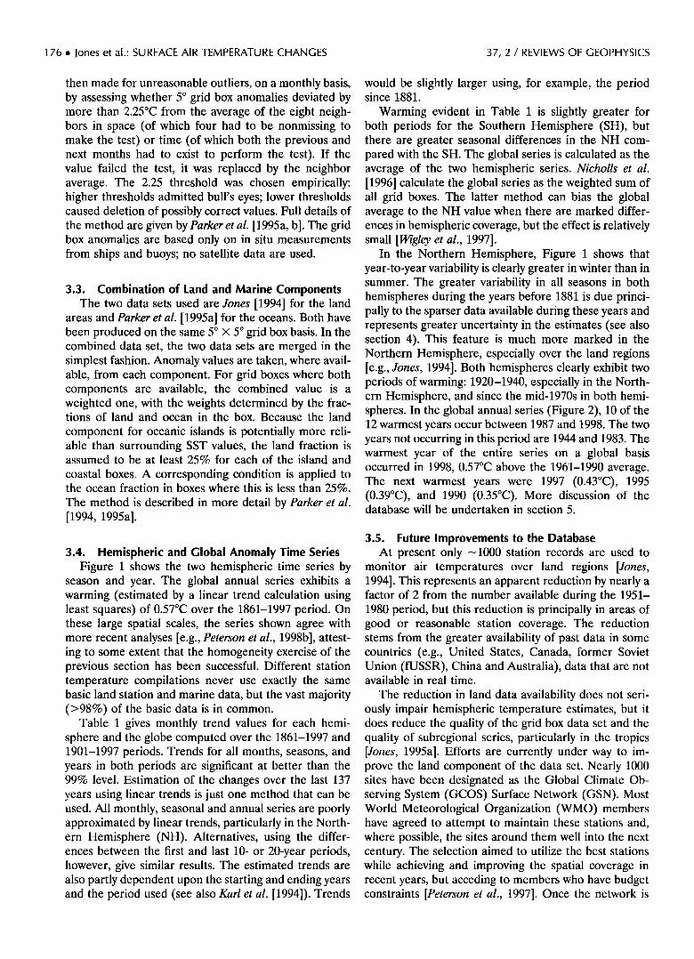
Figure 4. One and two standard errors (SE) on the hemispheric and global temperatures on the decadal timescale. The shaded areas highlight +__ 1 SE.

of stations with time in the individual grid box series but does not correct for it. Time series of individual grid box series will exhibit variance changes that may be unreal- istic and simply a result of changing station density. This factor is discussed more in section 5.

In midlatitude continental regions where there is great variability of temperature with time, s/2 will be higher than over less variable regions such as coastal areas, the oceans and tropics. In these continental regions, ?, which has a maximum value of 1, is lower (---0.8-0.9) than over oceanic and tropical regions (>0.9). Figure 3 illustrates this with the fields for s/2 and ?, calculated for annual data on the interannual timescale.

The value of ? is always greater than 0.7, for the 5 ø x 5 ø

grid box size, and thus never approaches zero when (1) would imply an SE value of zero. Jones et al. [1997a] show that an alternate assumption about the standard error (SE = s/2, for n = 0, instead of s•27) gives slightly larger values (by ---0.01-0.02) than those presented here.

The implications of the formula are that in any global SE assessment it is more important to have temperature estimates from continental regions, as opposed to oceanic regions, of the same size, because of the former regions' greater variability. If, for example, a limited network of sites were to be deployed to measure global temperature, a much greater percentage of them would be located over land than the land/ocean fraction would imply.

Figure 3 shows that the fields of s• 2 and ? are relatively


smooth on the annual timescale. This also applies on the monthly timescale, where ? falls to minimum values of about 0.7 in some regions in the winter season. Jones et al. [1997a] used these smooth features to enable values of these variables to be estimated for all grid boxes without temperature data. SE values for such grid boxes can then be estimated from Eq. (1)•with n = 0. The reliability of these assessments was tested using 1000- year control runs of general circulation models (GCMs), for which complete global fields of surface temperature data were available [Jones et al., 1997a].

With SE estimates for each grid box, which will vary in time due to data availability, we can calculate the average large-scale SE in a similar manner to the calculation of the large-scale average temperature anomalies,

Ng / Ng SE 2 - • SE• 2 cos (lati) • cos (lati) i=1 i=1

(2)

where Ng is the total number of grid boxes in the region under study. If all the grid boxes were independent of each other then the large-scale SE 2 would be SE e divided by the number of grid boxes. However, the effec- tive number of independent points (Neff) is considerably less than the total number of grid boxes and difficult to estimate. Neff has been discussed by earlier authors [e.g., Livezey and Chen, 1983; Briffa and Jones, 1993; Madden et al., 1993 and Jones and Briffa, 1996] and referred to also as the number of spatial degrees of freedom. Nef f values in Jones et al. [1997a] were estimated using the approach suggested by Madden et al. [1993].

The SE of the global, hemispheric or large-scale average is therefore

2

Smgloba I = sm2/Neff (3)

following an analogy from earlier work by Smith et al. [1994]. Typical values of Nef f depend on timescale, making comparisons between different studies difficult. Jones et al. [1997a], for annual data on the interannual timescale, obtain values of ---20 for both surface observations and similar fields from the control runs of

GCMs. Values increase to --•40 for seasonal series on

this timescale, with slightly higher values in the northern summer compared to the winter season. The timescale dependence of all the formulae means that the SE values must be calculated on the timescale of interest. SE values

on the decadal timescale are only marginally smaller than those calculated on the interannual timescale.

Figure 4 shows the global and hemispheric temperature values with appropriate standard errors on the decadal timescale. Given the greater percentage of missing regions in the Southern Hemisphere, the SE values are highest there. SE values decrease with time during the course of the last 150 years, reaching typical values for the globe during the last 50 years of 0.048øC (0.054) on the decadal (interannual) timescale. It must be remembered that these estimates are for sampling errors

only and do not include additional uncertainties that relate to the correction of SST bucket observations or to

any residual urbanization effects over some land areas.

5. ANALYSES OF THE SURFACE TEMPERATURE

RECORD

The record has been extensively analyzed over the last 10-15 years in a series of review papers or chapters in national and international reviews, including those for the IPCC [e.g., Wigley et al., 1985, 1986, 1997; Ellsaesser et al., 1986; Folland et al., 1990, 1992; Jones and Briffa, 1992; Jones, 1995a; Nicholls et al., 1996]. The hemispheric and global series and their trends have already been discussed in section 3.4. In this section we compare the two periods of twentieth century warming, 1925- 1944 and 1978-1997, and discuss trends in the areas affected by extreme warmth, trends in Arctic temperatures, trends in maximum and minimum temperatures, the apparent disagreement between recent warming measured at the surface and by satellites for the lower troposphere, and the last 150 years in the context of the millennium.

5.1. Comparison of the Two Twentieth-Century Warming Periods

Figures 1, 2, and 4 clearly indicate that most of the warming during this century occurred in two distinct periods. The periods differ between the hemispheres and among the seasons, but the periods from about 1920 to 1945 and since 1975 stand out. Plate 1 shows the trend

of temperature change by season for the two 20-year periods, 1925-1944 (Plate la) and 1978-1997 (Plate lb). The annual global temperature increases during the two periods were 0.37 and 0.32øC, respectively, with the second period on average 0.27øC warmer than the first.

In both periods, the regions with the greatest warming and cooling occur over the northern continents and, with the exception of a few isolated grid boxes, during the December-January-February (DJF), March-April-May (MAM), and September-October-November (SON) seasons. The warming is generally greatest in magnitude during the DJF and MAM seasons over the high latitudes of the northern continents, although these regions are not always those where local statistical significance is achieved. Small trends over some oceanic areas are

significant because of low variability in year-to-year temperature values. The 1978-1997 period has a much larger area with statistically significant warming compared with 1925-1944. The pattern of recent warming is strongest over northern Asia, especially eastern Siberia. It is also evident over much of the Pacific basin, western parts of the United States, western Europe, southeastern Brazil, and parts of southern Africa. The 1925-1944 warming was strongest over northern North America and is clearly evident over the northern Atlantic, parts of the western Pacific and central Asia. The improvements


in coverage between the two periods are apparent, and some shipping routes are surrounded by data voids in 1925-1944 (see also Parker et al. [1994]).

5.2. Trends in the Areas Affected by Extreme Warmth

The previous section shows that 20-year warmings were greatest over continental and high latitude regions where temperatures vary most on interannual timescales: extreme colors in Plate 1 are not apparent over the tropics and the oceans. The 95% significance levels on Plate 1, however, show that warming, particularly for the most recent 20 years, was just as significant in the less interannually and decadally varying regions compared with the highly variable regions. Recently, Jones et al. [1999] has transformed the surface temperature database from one in anomalies with respect to 1961-1990 to percentiles from the same time period. This enables the rarity of extreme monthly temperatures to be directly compared between grid boxes. The transformation was performed using gamma distributions, which treat each grid box impartially, accounting for the effects of both differences in interannual variability across the world, and differences in skewness.

Plate 2 compares the anomaly and the percentile method for displaying annual temperatures for the year 1998 (the year 1997 is shown by Jones et al. [1999, Figure 7]). The percentile map indicates unusual temperatures over many tropical and oceanic regions that would not warrant a second glance in the anomaly form. Similar maps could be constructed using the normal distribution, but seasonal and annual temperatures are often negatively skewed over many continental and high latitude regions. The gamma distribution also takes account of this.

Figure 5 shows the percentage of the analyzed area of the globe with annual temperatures greater than the ninetieth and less than the tenth percentile since 1900. An increase in the percentage of the analyzed areas with warm extremes is evident, but by far the greatest change is a reduction in the percentage of the analyzed area with cold extremes. Some caution should, however, be exer- cised when interpreting these results. Large changes in coverage have occurred over the twentieth century, so some of the changes may be due to areas entering the analysis during this time. Coverage changes are minimal, however, since 1951. Second, grid box values based on fewer stations or few individual SST observations, a more common situation at the beginning of the century, are more likely to be extreme in this percentile sense (see earlier discussion in section 4.2 and Jones et al. [1997a]). Again, changes in the density of observations per grid box are minimal since 1951. In future analyses it should be possible to correct for this second problem, producing grid box time series that do not have changes in variance due to changes in station or SST numbers, using some of the formulae developed by Jones et al. [1997a].

5.3. Trends in Arctic Temperatures There has been recent controversy regarding Arctic

temperature trends. We discuss in this section the three principal analyses. Chapman and Walsh [1993] examined the overall seasonal behavior of Arctic land station tem-

peratures between 1961 and 1990. Their results show that in winter and spring, warming dominated with values of about 0.25 and 0.5øC/decade respectively. In summer, the trend was near zero, and in autumn the trend either was neutral or showed a slight cooling. Consider- ing the longer record back to the mid nineteenth century [Jones, 1995c], only the spring season had its warmest years of the entire period recently, i.e., in the 1980s and 1990s.

For the temperature trends over the pack ice, there are two investigations [Kahl et al., 1993; Martin et al., 1997], which yield contradictory results. We refer to these as KCZ and MMD, respectively. For the western Arctic (70ø-80øN, 90ø-180øW) and the time period 1950-1990, KCZ used a combination of surface air temperature data determined from dropsonde data taken by the U.S. Ptarmigan flights for 1950-1961 and radiosonde data from the fUSSR-manned North Pole

(NP) drifting ice stations for 1954-1990 (data are discussed in more detail in section 6.4). From the combination of these two data sets, KCZ find a significant cooling trend of 1.2øC/decade in autumn and 1.1øC/ decade in winter, which contradicts the land-based studies. Walsh [1993, p. 300], however, observes "that only one [NP] track extends as far south as 75øN in the Western Arctic domain..." and that many of the dropsonde profiles were obtained from the climatologically warmer marginal ice zone, "... where all these (dropsonde) measurements were made in the first 12 years... of the study period." This implies that their observed cooling trends may be generated by the geographically warm bias of the dropsonde measurements. Another source of potential bias is the instrument time lag as the dropsonde falls through the Arctic inversion, and the fact that the NP radiosonde surface temperatures are always taken from multiyear ice or ice islands, while some of the dropsonde surface temperatures could be from open leads or thin ice.

Given the impact that the KCZ paper had on the science community, MMD searched for trends in the NP 2-m air temperature data for 1961-1990, where these temperatures were taken at 3-hour intervals inside a Stevenson screen, then resampled to 6-hour intervals. Their area of interest is an irregular region in the central Arctic, excluding the climatological warmer regions of the Beaufort Sea south of 77øN and the vicinity of Fram Strait. In their trend analysis, MMD used both the measured and anomaly fields, where the anomalies were the difference between the daily NP temperatures and the gridded mean daily field defined from optimal interpolation of the buoy, NP, and coastal station temperatures for 1979-1993 [Martin and Munoz, 1997]. The purpose in using the anomaly fields was to remove


90N

60N

30N

0

30S

60S

90S 180

Surface Temperature Anomalies (øC, w.r.t. 1961-90) 1998

ß

120W 60W 0 60E 120E 180

-5 -3 -1 -0.5 -0.2 0 0.2 0.5 1 3 5 Ocean: Parker et al (Climatic Change 199•) Land: Jones (J.Climate 1994)

Surface Temperature Anomaly Percentiles (w.r.t. 1961-90) 1998

• (Anomalies fitted to Gamma Distributions) I I I I I

90N' •_.•• • _•_ ,, .___ __ I 60N --•'-"X• '-'• '-"•'• x._/-- 30N "

0

30S x..

60S

90S •0 120W 60W 0 60E 120E 180

0 2 10 20 30 40 50 60 70 80 90 98 100

Plate 2. Surface temperatures for 1998, relative to the 1961-1990 average, expressed (a) as anomalies and (b) as percentiles. The percentiles were defined by fitting gamma distributions to the 1961-1990 annual deviations relative to the 1961-1990 average, for all 5 ø x 5 ø boxes with at least 21 years of annual data in this period.


1910 1920 1930 1940 1950 1960 1970 1980 1990

40 '

3O

2O

10

1910 1920 1930 1940 1950 1960 1970 1980 1990

Figure 5. Percentage of the monitored area of the globe, for each year from 1900 to 1998, with annual surface temperatures above the ninetieth percentile and below the tenth percentile. The percentiles were defined by fitting gamma distributions, based on the 1961-1990 period, using all 5 ø x 5 ø boxes with at least 21 years of data.

geographical inhomogeneities from the temperatures. For both fields, MMD found statistically significant warming to occur in May (0.8øC/decade) and June (0.4øC/decade), and on a seasonal basis, they found significant warming in the summer anomaly field (0.2øC/ decade). Although the other seasonal trends were not significant at the 95% level, MMD also found warming in winter (0.35øC/decade) and spring (0.2øC/decade), and a cooling in autumn (-0.2øC/decade). Their numbers are consistent with land stations (Chapman and Walsh [1993] and the data used in 5 ø grid box analyses here).

5.4. Trends in Maximum and Minimum

Temperatures Up to now all the surface temperature analyses pre-

sented in this paper have used monthly mean temperatures. This situation arises principally from the widespread availability of this variable. Over the last few decades, greater understanding of the causes of some of the changes has been gained by considering related changes in other variables, such as circulation and precipitation [e.g., Parker et al., 1994; Jones and Hulme, 1996]. Other temperature variables to receive similar widespread interest are the monthly mean maximum and minimum temperatures and their difference, the diurnal temperature range (DTR). These temperature extreme series have meaning only over land regions, and there are only enough data spatially to warrant analyses since about 1951. Longer data sets should exist back to the late nineteenth century but are available digitally for only a few countries (e.g., United States and fUSSR).

Karl et al. [1993b] were the first to extensively analyze trends in these variables, using gridded data covering 37% of the global land area. They found that for the 1951-1990 period, minimum temperatures warmed at 3 times the rate of maximum temperatures. DTR decreased over this period by 0.14øC/decade, while mean temperatures increased by 0.14øC/decade. Their study confirmed earlier studies for the United States [Karl et al., 1984]. Easterling et al. [1997] have extended this study

by including more data (54% of the global land areas) and extending the time series to 1993. (Until very recently, mean monthly maximum and minimum temperatures were not routinely exchanged between countries. This is one data set it is hoped will be dramatically improved through GCOS (see section 3.5).) This study confirmed the earlier study, showing that for nonurban stations over 1950-1993, minimum temperatures rose by 0.18øC/decade, maxima rose by 0.08 per decade, and the DTR decreased by 0.08øC per decade. The new study lowered the trend of minimum temperatures (0.18 compared with 0.21) somewhat by incorporating much more tropical station data. It also decreased the possibility of urbanization effects being the cause by using only nonurban stations in the analysis.

Plate 3 shows the trends for each 5 ø by 5 ø grid box on an annual basis for the 1950-1993 period. Minimum temperatures decrease in only a few areas, while the DTR decreases in most regions except Arctic Canada and some Pacific Islands. The new study made use of many regional assessments reported in a special issue of the journalAtmospheric Research [see Kukla et al., 1995].

5.5. Comparisons of Recent Surface Warming With Satellite Estimates

Figures l, 2, and 3, and Plates lb and 3 all indicate that surface temperatures have risen this century and particularly over the last 20 years or so. The increase is seen in most areas and is evident over land and marine

regions (see especially Plate lb). Recently, some doubt has been cast on the surface record by comparisons with satellite measures of the average temperature of the lower troposphere. The satellite record uses microwave sounding unit (MSU) instruments on the NOAA series of polar orbiters (see Christy et al. [1998] for the most recent review of the lower troposphere satellite record). Comparisons are usually made with the MSU2R record (which measures the weighted vertical temperature profile of the troposphere from the surface up to 250 hPa, centered on -750 hPa) but the original MSU2 record (surface up'to 200 hPa, centered on -500 hPa) is also

37, 2 / REVIEWS OF GEOPHYSICS Jones et al' SURFACE AIR TEMPERATURE CHANGES ß 187

Plate 3. Trends (in degrees Celsius per 100 years) for each 5 ø x 5 ø grid box for (a) maximum, (b) minimum, and (c) diurnal temperature range for nonurban stations. Redrawn with permission from Easterling et al. [1997]. Copyright 1997 American Association for the Advancement of Science.


....

•'.•

, , ..,. - .

0-3.0

_

C

Plate 3. (continued)

relevant [see Huh'ell and Trenberth, 1996, 1997, 1998]. The latter is known to have partial lower stratospheric influences [see Christy et al., 1998].

The doubt comes from the fact that over the 1979-

1996 period the surface warmed relative to MSU2R by 0.19øC per decade [Jones et al., 1997b]. Although neither the surface warming, the slight MSU2.R cooling, nor the difference is statistically significant, doubts have been cast on the veracity of the surface record since 1979 and, by inference, the pre-1979 period as well. The doubts are often expressed in the non-peer-reviewed, "grey literature," in newspaper articles, and on Web pages.

Several intercomparisons have been undertaken to unravel reasons for the differences [see, e.g. Christy et al., 1998; Hurrell and Trenberth, 1996, 1997, 1998; Jones et al., 1997b]. Several issues are undisputed in these studies. First, 20 years is too short a period over which to calculate trends and draw meaningful conclusions. Sec- ond, the two records are not the same, and their trends need not be equivalent. The records measure temperatures at different levels. At the surface, recent warming is greater in minimum temperatures, and the shallow nocturnal boundary layer over land areas is often de- coupled from the lower troposphere. More realistic comparisons with lower tropospheric temperatures might be made with maximum temperatures, but these are less spatially extensive. Also, because the MSU2R record is short, it may be possible for its trend to differ substantially from that for the surface without the two being physically incompatible.

Third, the MSU2R trend agrees almost exactly with radiosonde data [Parker e! al., 1997] aggregated together to mimic the equivalent vertical profile of MSU2R, with

a trend close to -0.04øC/decade. However, over the longer period from 1965 to 1996, the radiosonde record agrees with the surface (0.15øC/decade warming). Ra- diosonde records are known to contain many problems of long-term homogeneity [Parker et al., 1997, and references therein], but it does seem strange to concentrate on the 1979-1996 agreements between radiosondes and MSU2R and forgel the longer 32-year agreement between the radiosondes and the surface. Fourth, and often ignored in the comparisons, is the long-term agreement, both over this century and since 1979, between the !and and marine components of the surface record (see also section 2.2).

Several reasons have been postulated for the differences. The MSU2R record is an amalgamation of many different satellite series, each requiring calibration against each other as well as corrections for orbital decay of the satellite and possible drift in the satellite crossing times. Changes relative to the surface record were most noticeable during 1981-1982 and again during 1991 (both times of satellite changes); these may be at least partly instrumental and have been highlighted by Hurrell and Trenberth [1996, 1997, 1998] and Jones et al. [1997b]. There are no evident reasons for heterogeneity in the land or marine surface record at these dates. The

MSU2R-radiosonde agreement is generally good, although a similar comprehensive comparison similar to the surface-MSU2R assessment of Jones et al. [1997b] has yet to be carried out. Comparisons are usually carried out as zonal and hemispheric means. Hurrell and Trenberth [1998] show that local colocated comparisons show poor agreement over tropical continents. They also highlight the original MSU2 record, which shows a


warming of 0.05øC/decade over the 1979-1993 period. If the MSU2R is in error, the implication is that the radiosonde record must also contain errors. The reason

favored by Christy et al. [1998] is that the differences are real and represent differences in warming rates at different levels in the lower troposphere.

Recently, another potential inhomogeneity in the MSU2R record has been identified by Wentz and Schabel [1998]. It relates to the orbital decay of each satellite, which is driven by variations in solar activity causing variations in orbital drag. They calculate that on a global basis, the effect should result in a correction of the MSU2R data by +0.12øC/decade. The effect does not change other MSU channels, including the raw MSU2 data. J. R. Christy (personal communication, 1998) claims that the effect is already implicitly accounted for during the numerous intersatellite calibrations necessary to produce the continuous series since 1979. Santer et al. [1999], in an extensive study of tropospheric and stratospheric temperature trends from radiosondes, MSU data, and model-based reanalyses since 1958, indicate that all have potential biases and inhomogeneities such that the whole issue is unlikely to be resolved in the near future. Only comprehensive colocated comparisons of radiosondes and the MSU2R and greater understanding and correction of the biases in radiosondes will resolve

the issue. In many regions the necessary metadata, giving information on which sondes have been flown, are not always available.

5.6. The Last 150 Years in the Context of the Last

Millennium

The global surface temperature has clearly risen over the last 150 years (Figure 2 and Table 1), but what significance does this have when compared with changes over longer periods of time? The last millennium is the period for which we know most about the preinstrumental past, although it must be remembered that such knowledge is considerably poorer than for the post-1850 period. Information about the past comes from a variety of proxy climatic sources: early instrumental records back to the late seventeenth century, historical records, tree ring densities and widths, ice core and coral records (see Jones et al. [1998], Mann et al. [1998], and many references therein for more details). Uncertainties are considerably greater because information is available only from limited areas where these written or natural archives survive and, more importantly, because the proxy indicators are only imperfect records of past temperature change (see, e.g., Bradley [1985], Bradley and Jones [1993], and the papers in volumes such as those of Bradley and Jones [1995] and Jones et al. [1996]).

Over the last few years, a number of compilations of proxy evidence have been assembled following the pioneering work of Bradley and Jones [1993]. In Figure 6 we show three recent reconstructions of Northern Hemi-

sphere temperature for part of the last millennium. The reconstructions are all of different seasons (annual

0.0

-0.5

1200 1400 1600 1800 2000

1200 1400 1600 1800 2000

Figure 6. Northern Hemisphere temperature reconstructions from paleoclimatic sources. The three series are Mann et al. [1998, 1999] (thick), Briffa et al. [1998] (medium) and Jones et al. [1998] (thin). All three annually resolved reconstructions have been smoothed with a 50-year Gaussian filter. The fourth (thickest) line is the short annual instrumental record also smoothed in a similar manner. All series are plotted as depar- tures from the 1961-1990 average.

[Mann et al., 1998, 1999] and two definitions of summer [Briffa et al., 1998; Jones et al., 1998]). The short instrumental record on an annual basis is superimposed. Agreement with the annual instrumental record is poor- est during the nineteenth century, partly because of the different seasons (summer in two of the series) used. The instrumental record also rises considerably in the last 2 decades, and this cannot be seen in the multiproxy series because they end before the early 1980s, as some of the proxy records were collected during these years.

The most striking feature of the multiproxy averages is the warming over the twentieth century, for both its magnitude and duration. The twentieth century is the warmest of the millennium and the warming during it is unprecedented (see also discussion by Mann et al. [1998, 1999] and Jones et al. [1998]). The four recent years 1990, 1995, 1997, and 1998, the warmest in the instrumental series, are the warmest since 1400 and probably since 1000. The end of the recent E1 Nifio event (such events tend to warmer temperatures globally) and the greater likelihood of La Nifia (which tends to lead to cooler temperatures) as opposed to E1 Nifio conditions during 1999 and 2000 means that 1998 will likely be the warmest year of the millennium. The coolest year of the last 1000 years, based on these proxy records, was 1601. If standard errors could be assigned to this assessment, they would be considerably greater than errors given during the instrumental period [Jones et al., 1997a]. The standard errors given by Mann et al. [1998, 1999] may seem relatively small, but they only relate to their regressions and include neither the large additional uncertainties in some of the proxy records before the nineteenth century, nor the standard errors of the instrumental record.

Numerous paleoclimatic studies have considered the last millennium and two periods, the Little Ice Age


[Grove, 1988; Bradley and Jones, 1993] and the Medieval Warm Epoch [Hughes and Diaz, 1994], are often discussed. The latter two studies question perceived wisdom that these periods were universally colder and warmer, respectively, than the present. The questioning arises from the considerable advances in paleoclimatology that have been made over the past 15-20 years. The series used in Figure 6 contain from ten to several hundred Northern Hemisphere proxy climatic series, considerably more series than previously analyzed. The coldest century of the period since 1400, the seventeenth, was on average only 0.5ø-0.8øC below the 1961- 1990 base. The differences between these studies and

some earlier work is that they are based on considerable amounts of proxy data rather than individual series or schematic representations of perceived wisdom [Folland et al., 1990, Figure 7.1].

6. ANOMALY VERSUS ABSOLUTE TEMPERATURES

Throughout this review, temperature series have always been quoted in degrees Celsius with respect to the "normal" period 1961-1990. Earlier analyses used 1951- 1970 [Jones et al., 1986a, b] or 1951-1980 [Parker et al., 1994]. The only systematic differences between these analyses are simply changes in reference level, due to the different normal periods. There will, however, be random differences depending on the normal period, due to missing data values affecting the computation of the reference period means (see also Wigley et al. [1997]).

Anomaly values overcome most of the problems with absolute temperatures such as differences between stations in elevation, in observation times, the methods used to calculate monthly mean temperatures, and screen types. Any changes with time in these aspects should be corrected in the initial homogeneity assessment of a station temperature time series. Anomaly values should be all that are required in any analysis of the basic 5 ø x 5 ø grid box data set.

The first absolute temperature climatology was produced by Crutcher and Meserve [1970] for the NH and by Taljaard et al. [1969] for the SH. The 5 ø grid point values from these early works are available digitally. Data avaiI- ability must have been poorer then than now. Also, these earlier analyses must be based on few years of record in data sparse regions such as Antarctica and parts of the tropics, making it difficult for each region to be based on a consistent common period.

Recent work, however, has enabled absolute temperatures for the 1961-1990 period to be much better defined, using considerably enhanced data sets. In this section we produce a globally complete analysis of the absolute value of surface temperature for a common period, 1961-1990. Our absolute climatology is made up of four components: land areas excluding Antarctica, oceanic areas from 60øN to 60øS, Antarctica poleward of 60øS, and northern oceanic areas including the Arctic,

north of 60øN. The four components are discussed sep- arately.

6.1. Land Areas Excluding Antarctica For these regions we make use of the 1961-1990

climatology developed from station data by New et al. [1999]. In this analysis, 12,092 station estimates of mean temperature for 1961-1990 are used to construct a 0.5 ø latitude by 0.5 ø longitude climatology for global land areas excluding Antarctica. The temperature averages were given reliability codes, expressed as a percentage of the number of years available during the 1961-1990 period. In regions of dense coverage, stations with higher percentages were used preferentially. For most stations, mean temperature was calculated as the average of maximum and minimum temperature, thus avoid- ing potential differences due to the method of calculating mean temperature (see discussion in section 2.1).

The station data were interpolated as a function of latitude, longitude, and elevation using thin plate splines [e.g., Hutchinson, 1995]. The use of elevation enabled the splines to define spatially varying temperature lapse rates in different mountainous areas, provided that the basic data were adequate (see New et al. [1999] for further discussion of this point). Station data were insufficient to achieve spatially varying lapse rates in Ant- arctica and Greenland (see later in sections 6.3 and 6.4). The elevation data used originated from a 5-min digital elevation model (DEM), available from the National Geophysical Data Center (NGDC) (see Acknowledg- ments) which had been degraded to 0.5 ø cells by averaging the thirty-six 5-min pixels in each cell. The accuracy of the interpolations has been assessed using cross- validation and by comparison with earlier climatologies (see references of New et al. [1999]). We believe this climatology represents an important advance over previous work in that it is strictly constrained to the period 1961-1990, elevation is explicitly incorporated, and errors are evaluated on a regional basis.

For combination with the other three components, the 0.5 ø x 0.5 ø resolution was degraded to 1 ø x 1 ø. In this degradation, four 0.5 ø x 0.5 ø cells were averaged to give one 1 ø cell. The DEM was also degraded to provide a 1 ø elevation field for all land areas.

6.2. Oceanic Areas From 60øN to 60øS

In the anomaly data set we used SST anomalies over marine regions because of their superior accuracy compared with MAT data. For the climatology, however, it is preferable to use MAT, as MAT should match better with land temperature on islands and from coastlines than an SST climatology.

MAT climatologies, however, will be affected by solar heating on board ship (see section 2.2). To overcome this problem, we combined a new SST climatology for 1961-1990 [Parker et al., 1995b] with an air-sea temperature difference climatology, also for 1961-1990. The SST climatology makes use of all available in situ and


satellite SST data during the period, new marginal sea ice zone SST estimates, and new Laplacian-based adjust- ment schemes [Reynolds, 1988] in areas where there were insufficient data to produce a true climatology. The air-sea temperature difference data used similar infilling techniques but made use of only NMAT and in situ SST values from 1 hour before local sunset to 1 hour after

local sunrise, to minimize the effect of solar heating on ships' MAT. In the development of the air-sea temperature difference climatology, we assume that values based on nighttime-only values are the same as those based on all 24 hours of the day. Both climatologies are available on a 1 ø x 1 ø resolution. Our air temperature version is the sum of the air-sea and the SST climatol-

ogy.

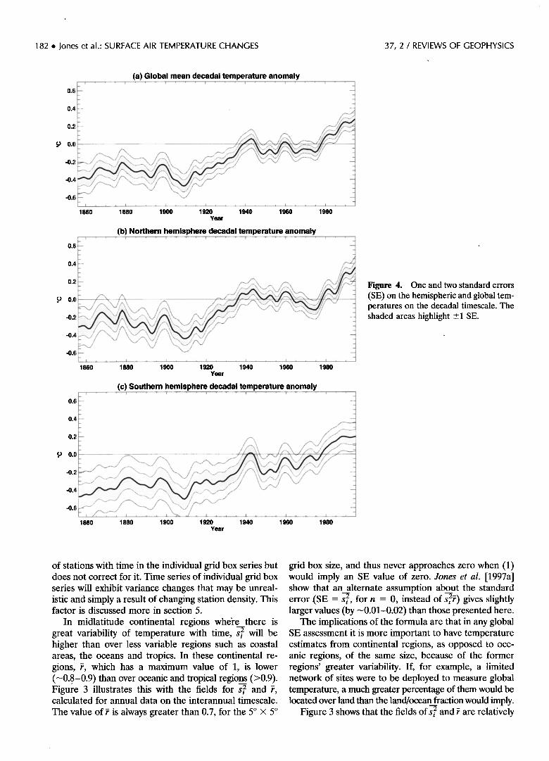
Plate 4 illustrates this climatology combined with the land data for the four midseason months for the region 60øN to 60øS. At this contour resolution, most of the large spatial changes are due to latitude, elevation, and land-ocean contrasts. The latter are markedly stronger in the winter hemisphere but are still evident in the transition seasons in some areas.

6.3. Antarctica Poleward of 60øS

For this region, average temperatures for 35 stations were collected from similar sources to those given by New et al. [1999]. Only 15 were near complete for the 1961-1990 period, the remaining 20 being either from sites with records for part of 1961-1990 or from locations with data only in the 1950s. Additional sources included a number of Antarctic data publications from countries operating the stations (e.g., Schwerdtfeger et al. [1959], Japan Meteorological Agency [1995], and sources listed by Jones [1995b]). In a few years' time it should be possible to increase the number of sites available by using the then extended information from automatic weather stations (AWSs). A number of new AWS sites are located in regions considerable distances from manned stations [Steams et al., 1993]. As yet, though, record lengths are too short.

The monthly station temperature normals were interpolated using the same spline software as the other land areas. Only four of the 35 stations are located at eleva- tions in excess of 1500 m, the remainder being at eleva- tions below 300 m. This was too sparse a network for a full three-dimensional interpolation. Elevation was therefore used as a covariate rather than a truly independent variable, enabling the definition of monthly continent-wide relationships with elevation. These lapse rates varied monthly from 8 (summer) to 11 (winter) øC km -•, larger than would be expected. This is most likely due to the strong covariance of elevation and position, i.e., elevation increases and temperature decreases pole- wards. The interpolation assigned more weight to elevation than position. The interpolation over land was extended over adjacent ocean areas (sea ice areas for part of the year) to 60øS, where the MAT climatology provided the northern boundary. The use of such a control

results in a linear increase in temperature between the ice sheet margin and 60øS. In reality, the field is likely to exhibit a sharp increase in air temperature at the margin of the continental ice sheet, although this step will be smoothed out to some extent by using 30-year averages.

Plate 5 illustrates the Antarctic climatology for the four midseason months. Even at the relatively coarse resolution, the influence of the sea ice can be seen, principally by its absence during January. The strong gradients across the Antarctic Peninsula during summer and autumn are evident as well as the coastal-sea ice

extent effects in the Weddell and Ross Seas and Prydz Bay.

6.4. Arctic Areas North of 60øN

In this region, data for land areas come from the New et al. [1999] climatology. There are considerably more stations in this region than in the Antarctic, although there is only one high-elevation station in the interior of Greenland (and even this is for a relatively short period of record). As with Antarctica, elevation over Greenland could be incorporated only as a covariate. Elsewhere in the Arctic, elevation was as an independent variable and followed New et al. [1999].

The most difficult part of this region is the Arctic Ocean and the extensive sea ice regions in the northern Atlantic and Pacific Oceans. The systematic collection of temperature data within the pack ice of the Arctic basin began with Nansen's drift across the Arctic in the Fram during 1893-1896. During this drift, temperatures were recorded at 6-hour intervals. Sverdrup [1933] describes a similar time series that was taken during the 1919-1926 Maud drift, where the temperature record extends from August 1922 to September 1924. Sverdrup [1933] combined these two sets of drift observations with land

station observations and published the first monthly climatology for the basin.

In 1938, the fUSSR began their series of North Pole station ice camps, which were oceanographic and meteorological stations established by aircraft on either multiyear ice floes or ice islands in the central Arctic [Colony et al., 1992]. The series began with NP-1, which gathered data from May 1938 to March 1939. Following World War II, NP-2 gathered during April 1950 to April 1951; then in 1954 the establishment of NP-3 marked the

beginning of the continuous occupation of the basin, where the fUSSR maintained 1-4 stations until April 1991, when NP-31 was recovered. The NP 2-m air temperatures were taken at 3-hour intervals inside a Steven- son screen. They have recently been resampled to every 6 hours and are available on CD-ROM from the Na-

tional Snow and Ice Data Center (NSIDC). During the NP period the United States and Canada also carried out a series of shorter-term occupations of ice floes and ice islands; these records are available from the NCDC.

The next major set of temperature observations began on January 19, 1979, as the part of the U.S. contri- bution to the First Global Atmospheric Research Pro-

192 ß Jones et al.' SURFACE AiR TEMPERATURE CHANGES 37, 2 / REVIEWS OF GEOPHYSICS

gram (GARP) Global Experiment (FGGE), and consisted of an array of air-dropped, satellite-tracked buoys [Thomdike and Colony, 1980]. The purpose of these buoys was to record both the large-scale ice deformation by determining the buoy position, and the pressure field driving this deformation. A temperature sensor was included only to aid in the pressure sensor calibration. The instruments were mounted inside a ven-

tilated 0.6-m-diameter spherical hull. This program was known as the Arctic Ocean Buoy Program until 1991, when to reflect the growing contributions from other nations, the program name was changed to the Interna- tional Arctic Buoy Program (IABP). Since 1979 a large number and variety of buoys have been deployed by parachute, aircraft landings, ship, and submarine. Begin- ning in 1985 the program began the installation of buoys having ventilated and shielded thermistors at 1-2 m (R. L. Colony, private communication, 1998). As illus- trated on the IABP Web site (see acknowledgments), a large variety of designs were deployed, with both inter- nal and external thermistors. Today buoys with external and radiation shielded thermistors mounted at 2-m

height are deployed as much as possible. As Martin and Munoz [1997] describe, there is a

general problem with the buoy thermistors during summer, which became apparent when the buoy summer means were compared with the NP means. For the air temperature measurements above thick sea ice, a natural calibration period occurs in summer. The reason for this is as follows: at the beginning of summer, because of the natural sea ice desalination cycle, the upper ice surface is virtually salt free. Then as summer progresses, freshwater melt ponds form on the ice surface, so that the air temperature measurements above the ice are provided with a natural calibration point that is very close to 0øC. From the Fram and Maud data, Sverdrup [1933] first described this isothermal period. From analysis of those NP stations north of 82øN, Martin et al. [1997] found for the period June 23 to July 31 a mean temperature of -0.2øC with a standard deviation of 0.9øC.

Martin and Munoz [1997] found that most of the individual buoys for the same region and for the summer period had m•ean temperatures that were 1ø-3øC above freezing, or much warmer than the means of the NP temperatures. We attribute this temperature increase to solar heating of the thermistors. Out of 261 buoys deployed during the period 1979-1993, only 29 had a mean temperature that fell within one standard deviation of the NP summer mean, and only four buoys lay within half a standard deviation. Of the remainder, only four had a cold bias, so that 229 buoys had a warm bias. Informal investigations by two of us (S.M. and I.R.) show that the problem with summer overheating contin- ues through the 1997 summer. In spite of this problem, Martin and Munoz [1997] used a variety of filtering techniques to remove these summer offsets, then used an optimal interpolation scheme for the NP, buoys and coastal land station temperatures, assuming a constant

correlation decay length of 1300 km, to produce a 12- hour, 200-km gridded temperature field for the basin for the 1979-1994 period.

Building upon this work, Rigor et al. [1999] studied the monthly mean dependence of the correlation length scales. Although they find that during autumn, winter, and spring, their correlation length scales approximately equal the Martin and Munoz value, during summer the correlation length scales are smaller than during other seasons, and much smaller between the coastal land and ice temperatures than between the different ice temperatures, i.e., the buoy or NP temperatures. They used these length scale estimates to derive an improved optimal interpolation data set called IABP/POLES, which provides 12-hour temperatures on a 100-km rectangular grid, for 1979-1997. In this analysis the summer buoy data were also adjusted to match the NP statistics. Rigor et al. find that the IABP/POLES data set has higher correlations and lower biases compared with the NP and land station observations than the POLES data, and provides better temperature estimates especially during summer in the marginal ice zones. The IABP/POLES data set is available from the IABP Web site.

We use this new analysis for the Arctic Ocean for the years 1979-1997 and combine it with the land data north of 60øN from New et al. [1999] and the marine air temperatures north of 60øN in the northern Pacific and Atlantic Oceans. The Arctic Ocean analyses are therefore based on a slightly more recent period, but the quality of the 1979-1997 data for the region justifies this. Any temperature change between these two periods over this region is thought to be minimal (see section 5.3). Plate 6 illustrates the derived climatology for the Arctic for the four midseason months of January, April, July, and October. The coolest parts of the Arctic are over the land regions of northern Canada and eastern Siberia. Over the central Arctic in winter, temperatures are coldest across the region joining the coldest land regions. In the summer season, the Arctic Ocean is near 0øC almost everywhere, as may be expected from the previous discussion. The influence of the warm North Atlantic waters is evident in all the seasonal plots except summer.

6.5. Combination of the Four Components Into the 1961-1990 Climatology of Surface Air Temperatures

Combination of the analyses for the various domains was achieved in the most straightforward manner. For the zone 60øN to 60øS, the climatological value for each 1 ø square is selected from either the land or the marine analysis. If both analyses were available, the average of the two was taken. The two separate analyses for the Arctic and Antarctic regions were then combined. The climatology available on a 1 ø x 1 ø basis, together with the surface DEM used, can be found at the Climatic Research Unit Web site (see acknowledgments).

It is now a trivial task to calculate the mean hemi-

spheric and global temperatures for the 1961-1990 pe-

37, 2 / REVIEWS OF GEOPHYSICS Jones et al' SURFACE AIR TEMPERATURE CHANGES ß 193

60N

30N _

0

30S

60S

180W

60N

30N _

o

3os.

ß

60S

180W

60N

30N

0

30S

60S

180W 60N

..•

30N

0

30S

ß t f !

135W 90W 45W

I ! I

135w 90w 45w

135w 90w 45w

z c

f • f

0 45E 90E 135E 180E

I I ! I

0 45E 90E 135E 180E

0 45E 90E 135E 180E

" o o

t 0

60S

180W 135W 90W 45W 0 45E 90E 135E 180E

-40 -30 -20 -10 -5 0 5 10 15 20 25 30

... : ......

Plate 4. Climatological values of average air temperature for the 1961-1990 period for the midseason months of January, April, July, and October for the region 60øN to 60øS.


JANUARY

0

% 08[

APRIL

JULY

0

o O3 I"/1 O3

OCTOBER

m

t

08 I. 08 I.

-80 -50 -30 -20 -15 -10 -5 -2 0 2 5 10 15 20

Plate 5. Climatological values of average air temperature for the 1961-1990 period for midseason months of January, April, July, and October for the Antarctic region south of 60øS.


JANUARY

10

APRIL

1:0

Jb.,... '•

ß

o ill

JULY

10

o•o C

OCTOBER

1!•o •

ITI

[' ,

! !

-80 -50 -30 -20 -15 -10 -5 -2 0 2 5 10 15 20

Plate 6. Climatological values of average air temperature for the 1961-1990 period for midseason months of January, April, July, and October for the Arctic region north of 60øN.

196 ß Jones et al' SURFACE AIR TEMPERATURE CHANGES 37, 2 / REVIEWS OF GEOPHYSICS

25

2O

GLO _

_

_

_ NH _

_

_

_

_

_

JAN FEB MAR APR MAY JUN

i i i i

GLO- _

_

NH _

_

_

_

_

_

_

_

JUL AUG SEP OCT NOV DEC

Figure 7. Seasonal cycle of hemispheric and global mean temperatures in absolute degrees Celsius based on the 1961-1990 period.

riod. The average global annual temperature is 14.0øC, with the NH warmer than the SH (14.6øC compared with 13.4øC). In the Crutcher and Meserve [1970] and Taljaard et al. [1969] atlas climatologies the global average is 14.1øC (NH, 14.9øC; SH, 13.3øC). Given the warmth of the 1961-1990 period compared with earlier periods (--• 1931-1965) used by these workers, the differences are less than 0.5øC. We would expect our climatology to be about 0.2øC warmer than the earlier ones if climatic

changes were the only causes of the differences. New et al. [1999] have estimated cross-validation er-

rors for their climatology over large regional land areas. Typical errors are in the range 0.5ø-1.0øC, the larger values occurring over either data sparse regions or areas with complex terrain. Because there are potentially greater errors in our climatology over the Southern Ocean and Antarctica, due to sparse and incomplete (with respect to 1961-1990) data and the slightly different Arctic Ocean base period, we have not attempted to estimate standard errors for the climatology. Compari- son with the earlier climatologies suggests that the value of 14øC is within 0.5øC of the true value.

Figure 7 shows the annual cycle of temperatures in the two hemispheres and the globe. The magnitude of the hemispheric seasonal cycle is 13.1øC in the NH and 5.7øC in the SH. In the NH the warmest and coldest

months are the expected July and January. In the SH, January is warmest, but August rather than July is the coldest.

7. SUMMARY

We have reviewed a surface air temperature data set and produced a climatology of surface temperatures on a 1 ø x 1 ø basis based, as best as can be achieved, on data

from the 1961-1990 period. Our main conclusions are as follows:

1. Annual global surface temperatures warmed by 0.57øC over the period 1861-1997 and by 0.62øC over 1901-1997. Over both periods the warming was slightly greater in the SH than in the NH.

2. The measured temperature trends on a hemispheric basis are not very dependent upon the method used to combine the basic land and oceanic data, provided that all the basic data have been adequately adjusted for various inhomogeneities.

3. The warmest years of the record all occur in the 1990s. The four warmest years, in descending order, are 1998 (0.57øC above the 1961-1990 average), 1997 (0.43øC above average), 1995 (0.39øC above average) and 1990 (0.35øC above average).

4. The errors of estimation, due to sampling, are dependent upon the timescale of interest. On the interannual timescale, recent individual global mean, annual mean temperature anomalies have standard errors of. _0.05øC.

5. Patterns of warming over the two major warming periods in this century (1925-1944 and 1978-1997) indicate that the warming has been greatest over the northern continents and in the DJF and MAM seasons.

The warming over the earlier period was slightly greater (0.37øC compared with 0.32øC) on a global basis. The recent warming has been accompanied by increases in areas affected by significantly warm temperatures and reductions in the areas affected by significantly cool temperatures.

6. A recent reanalysis of Arctic temperature data from the pack ice areas indicates a slight warming on an annual basis with statistically significant warming over the 1961-1990 period in May and June.

7. The recent increase in mean temperature is the


result of stronger warming in nighttime compared with daytime. Over the 1950-1993 period, nighttime (minimum) temperatures have warmed by 0.18øC per decade and daytime (maximum) temperatures have warmed by 0.08øC per decade.

8. Recent surface temperature increases since 1979 have not been observed by satellite retrievals of lower tropospheric temperatures. Much has been written and said on this issue, highlighting the agreement between satellite and radiosonde measurements of lower tropospheric temperatures over the same period. However, surface and lower tropospheric temperature changes can and do differ, and the available databases are not yet good enough to estimate confidently the magnitude of possible differences over this near-20-year period. The agreement between surface and lower tropospheric temperature trends from radiosondes over the longer 1965- 1997 period is generally conveniently forgotten in many commentaries.

9. Proxy evidence for the preinstrumental period provides our only estimates of temperature capable of putting the period since 1851 into a longer-term context. The most recent proxy compilations indicate that the twentieth century was the warmest of the millennium and that the warming during it was unprecedented since 1400. The coldest century of the millennium was the seventeenth, with a temperature average only 0.5ø-0.8øC below the 1961-1990 average.

10. The 1 ø x 1 ø climatology, developed for surface air temperature, indicates an average global temperature of 14.0øC (14.6øC in the NH and 13.4øC in the SH).

ACKNOWLEDGMENIS. The authors thank Alan Rob-

ock for suggesting this review, and Chris Folland, Mike Hulme, Tim Osborn, the technical reviewers of Reviews of Geophysics for suggestions that improved it. Briony Horton is thanked for producing Figure 6 and assistance with Figure 7. This work has been supported by a number of research programs. P.D.J. acknowledges the support of the U.S. Department of Energy (grant DE-FG02-98ER62601). M.N. has been supported by the U.K. Natural Environment Research Council (grant GR3/09721). Much of the data collection of climatological (1961-1990) data has been supported by the U.K. Department of Environment, Transport, and the Regions (contract EPG 1/1/48). The development of the GISST2.2 sea surface temperature and sea ice climatology has been supported by the U.K. Public Meteorological Service Contract. S.M. and I.R. both gratefully acknowledge the support of NASA grant NAGS- 4375, Polar Exchange at the Sea Surface. I.R. also acknowledges the support of the United States Inter-Agency Buoy Program (USIABP) through grant N00014-96-C-0185. Many of the data sets upon which some of the figures depend, together with the climatology, are available on the Climatic Research Unit, University of East Anglia, Web site (http:// www.cru.uea.ac.uk/). The Arctic buoy data are also available from the IABP Web site (http://iabp.apl.washington.edu). The DEM is available from the NGDC Web site (http://www.ngdc. noaa.gov/seg/topo).

REFERENCES

Afifi, A. A., and S. P. Azen, Statistical Analysis: A Computer Orientated Approach, 2nd ed., 442 pp., Academic, San Diego, Calif., 1979.

Alexandersson, H., and A. Moberg, Homogenization of Swed- ish temperature data, I, A homogeneity test for linear trends, Int. J. Climatol., 17, 25-34, 1997.

Bradley, R. S., Quaternary Paleoclimatology: Methods of Paleo- climatic Reconstruction, 472 pp., Allen and Unwin, Win- chester, Mass., 1985.

Bradley, R. S., and P. D. Jones, Data bases for isolating the effects of the increasing carbon dioxide concentration, in Detecting the Climatic Effects of Increasing Carbon Dioxide, edited by M. C. MacCracken and F. M. Luther, pp. 29-53, U.S. Dep. of Energy, Washington, D.C., 1985.

Bradley, R. S., and P. D. Jones, "Little Ice Age" summer temperature variations: Their nature and relevance to recent global warming trends, Holocene, 3, 367-376, 1993.

Bradley, R. S., and P. D. Jones (Eds.), Climate Since A.D. 1500, 706 pp., Routledge, London, 1995.

Briffa, K. R., and P. D. Jones, Global surface air temperature variations over the twentieth century, 2, Implications for large-scale palaeoclimatic studies of the Holocene, Holo- cene, 3, 165-179, 1993.

Briffa, K. R., P. D. Jones, F. H. Schweingruber, and T. J. Osborn, Influence of volcanic eruptions on Northern Hemi- sphere summer temperatures over 600 years, Nature, 393, 450-455, 1998.

Chapman, W. L., and J. E. Walsh, Recent variations of sea ice and air temperature in high latitudes, Bull. Am. Meteorol. Soc., 74, 33-47, 1993.

Christy, J. R., R. W. Spencer, and E. Lobl, Analysis of the merging procedure for the MSU daily temperature time series, J. Clim., 11, 2016-2041, 1998.

Colony, R., I. Appel, and I. Rigor, Surface air temperature observations in the Arctic Basin, Tech. Memo. TM 1-92, Appl. Phys. Lab., Univ. of Wash., Seattle, 1992.

Conrad, V., and L. D. Pollak, Methods in Climatology, 459 pp., Harvard Univ. Press, Cambridge, Mass., 1962.

Crutcher, H. L., and J. M. Meserve, Selected-level heights, temperatures, and dew point temperatures for the Northern Hemisphere, NAVAIR 50-1C-52 rev., U.S. Navy, Chief Na- val Operations, Washington, D.C., 17 pp. plus charts, 11 pp. + 18 figs., 144 charts, 1970.

Easterling, D. R., and T. C. Peterson, A new method for detecting and adjusting for undocumented discontinuities in climatological time series, Int. J. Climatol., 15, 269-377, 1995.

Easterling, D. R., B. Horton, P. D. Jones, T. C. Peterson, T. R. Karl, D. E. Parker, M. J. Salinger, V. Razuvayev, N. Plum- ruer, P. Jamason, and C. K. Folland, Maximum and minimum temperature trends for the globe, Science, 277, 364-367, 1997.

Ellsaesser, H. W., M. C. MacCracken, J. J. Walton, and S. L. Grotch, Global climatic trends as revealed by the recorded data, Rev. Geophys., 24, 745-792, 1986.

Folland, C. K., and D. E. Parker, Corrections of instrumental biases in historical sea surface temperature data, Q. J. R. Meteorol. Soc., 121,319-367, 1995.

Folland, C. K., and M. J. Salinger, Surface temperature trends in New Zealand and the surrounding ocean, 1871-1993, Int. J. Climatol., 15, 1195-1216, 1995.

Folland, C. K., T. R. Karl, and K. Ya. Vinnikov, Observed climate variations and change, in Climate Change: The IPCC Scientific Assessment, edited by J. T. Houghton, G. J. Jenkins, and J. J. Ephraums, pp. 195-238, Cambridge Univ. Press, New York, 1990.

Folland, C. K., T. R. Karl, N. Nicholls, B. S. Nyenzi, D. E. Parker, and K. Ya. Vinnikov, Observed Climate Variability and Change, Climate Change 1992: The Supplementary Re-


port to the IPCC Scientific Assessment, edited by J. T. Houghton, B. A. Callander, and S. K. Varney, pp. 135-170, Cambridge Univ. Press, New York, 1992.

Folland, C. K., M. J. Salinger, and N. Rayner, A comparison of annual South Pacific island and ocean surface temperatures, Weather Clim., 17, 23-42, 1997.

Grove, J. M., The Little Ice Age, 498 pp., Methuen, New York, 1988.

Hansen, J. E., and S. Lebedeff, Global trends of measured surface air temperature, J. Geophys. Res., 92, 13,345-13,372, 1987.

Hughes, M. K., and H. F. Diaz, Eds., The Medieval Warm Period, Clim. Change, 26, 109-342, 1994.

Hurrell, J. W., Decadal trends in the North Atlantic Oscillation and relationships to regional temperature and precipitation, Science, 269, 676-679, 1995.

Hurrell, J. W., and K. E. Trenberth, Satellite versus surface estimates of air temperature since 1979, J. Clim., 9, 2222- 2232, 1996.

Hurrell, J. W., and K. E. Trenberth, Spurious trends in satellite MSU temperatures from merging different satellite records, Nature, 386, 164-167, 1997.

Hurrell, J. W., and K. E. Trenberth, Difficulties in obtaining reliable temperature trends: Reconciling the surface and satellite Microwave Sounding Unit records, J. Clim., 11, 945-967, 1998.

Hutchinson, M. F., Interpolating mean rainfall using thin plate smoothing splines, Int. J. Geogr. Inf Syst., 9, 385-403, 1995.

James, R. W., and P. T. Fox, Comparative sea-surface temperature measurements, Mar. Sci. Affairs Rep. 5, WMO 336, 27 pp., World Meteorol. Organ., Geneva, 1972.

Japan Meteorological Agency, Antarctic Meteorological Data, Spec. VoL VI, 364 pp., Tokyo, 1995.

Jones, P. D., Hemispheric surface air temperature variations: A reanalysis and an update to 1993, J. Clim., 7, 1794-1802, 1994.

Jones, P. D., Land surface temperatures•Is the network good enough?, Clim. Change, 31,545-558, 1995a.

Jones, P. D., Recent variations in mean temperature and the diurnal temperature range in the Antarctic, Geophys. Res. Lett., 22, 1345-1348, 1995b.

Jones, P. D., Temperature change in the Arctic and the Ant- arctic from instrumental and high-frequency paleoclimatic (since 1400) reconstructions, in Wadati Conference on Global Change and the Polar Climate, pp. 5-8, Inst. of Geosci., Univ. of Tsukuba, Tsukuba, Japan, 1995c.

Jones, P. D., and K. R. Briffa, Global surface air temperature variations during the twentieth century, 1, Spatial, temporal and seasonal details, Holocene, 2, 165-179, 1992.

Jones, P. D., and K. R. Briffa, What can the instrumental record tell us about longer timescale paleoclimatic reconstructions?, in Climatic Variations and Forcing Mechanisms of the Last 2000 Years, edited by P. D. Jones, R. S. Bradley, and J. Jouzel, pp. 625-644, Springer-Verlag, New York, 1996.

Jones, P. D., and M. Hulme, Calculating regional climatic time series for temperature and precipitation: Methods and il- lustrations, Int. J. Climatol., 16, 361-377, 1996.

Jones, P. D., S.C. B. Raper, B. D. Santer, B. S. G. Cherry, C. M. Goodess, P.M. Kelly, T. M. L. Wigley, R. S. Bradley, and H. F. Diaz, A Grid Point Surface Air Temperature Data Set for the Northern Hemisphere, Tech. Rep. TR022, 251 pp., U.S. Dep. of Energy, Washington, D.C., 1985.

Jones, P. D., S.C. B. Raper, R. S. Bradley, H. F. Diaz, P.M. Kelly, and T. M. L. Wigley, Northern Hemisphere surface air temperature variations: 1851-1984, J. Clim. Appl. Me- teorol., 25, 161-179, 1986a.

Jones, P. D., S.C. B. Raper, and T. M. L. Wigley, Southern HemiSphere surface air temperature variations: 1851-1984, J. Clim. Appl. Meteorol., 25, 1213-1230, 1986b.

Jones, P. D., S.C. B. Raper, C. M. Goodess, B. S. G. Cherry, and T. M. L. Wigley, A Grid Point Surface Air Temperature

Data Set for the Southern Hemisphere, Tech. Rep. TR027, 73 pp., U.S. Dep. of Energy, Washington, D.C., 1986c.

Jones, P. D., P.M. Kelly, C. M. Goodess, and T. R. Karl, The effect of urban warming on the Northern Hemisphere temperature average, J. Clim., 2, 285-290, 1989.

Jones, P. D., P. Ya. Groisman, M. Coughlan, N. Plummet, W.-C. Wang, and T. R. Karl, Assessment of urbanization effects in time series of surface air temperatures over land, Nature, 347, 169-172, 1990.

Jones, P. D., R. S. Bradley, and J. Jouzel (Eds.), Climatic Variations and Forcing Mechanisms of the Last 2000 Years, 649 pp., Springer-Verlag, New York, 1996.

Jones, P. D., T. J. Osborn, and K. R. Briffa, Estimating sampling errors in large-scale temperature averages, J. Clim., 10, 2548-2568, 1997a.

Jones, P. D., T. J. Osborn, T. M. L. Wigley, P.M. Kelly, and B. D. Santer, Comparisons between the microwave sounding unit temperature record and the surface temperature record from 1979 to 1996: Real differences or potential discontinuities?, J. Geophys. Res., 102, 30,135-30,145, 1997b.

Jones, P. D., K. R. Briffa, T. P. Barnett, and S. F. B. Tett, High-resolution palaeoclimatic records for the last millennium: Interpretation, integration and comparison with general circulation model control run temperatures, Holocene, 8, 455-471, 1998.

Jones, P. D., E. B. Horton, C. K. Folland, M. Hulme, D. E. Parker, and T. A. Basnett, The use of indices to identify changes in climatic extremes, Clim. Change, in press, 1999.

Kagan, R. L., Averaging of Meteorological Fields, 379 pp., Klu- wet Acad., Norwell, Mass., 1997.

Kahl, J. D., D. J. Charlevoix, N. A. Zaitseva, R. C. Schnell, and M. C. Serreze, Absence of evidence for greenhouse warming over the Arctic Ocean in the past 40 years, Nature, 361, 335-337, 1993.

Karl, T. R., and P. D. Jones, Urban bias in area-averaged surface air temperature trends, Bull. Am. Meteorol. Soc., 70, 265-267, 1989.

Karl, T. R., G. Kukla, and J. Gavin, Decreasing diurnal temperature range in the United States and Canada from 1941-80, J. Clim. Appl. Meteorol., 23, 1489-1504, 1984.

Karl, T. R., J. D. Tarpley, R. G. Quayle, H. F. Diaz, D. A. Robinson, and R. S. Bradley, The recent climate record: What it can and cannot tell us, Rev. Geophys., 27, 405-430, 1989.

Karl, T. R., P. Ya. Groisman, R. W. Knight, and R. R. Heim Jr., Recent variations of snow cover and snowfall in North America and their relation to precipitation and temperature variations, J. Clim., 6, 1327-1344, 1993a.

Karl, T. R., P. D. Jones, R. W. Knight, G. Kukla, N. Plummet, V. Razuvayev, K. P. Gallo, J. Lindesay, R. J. Charlson, and T. C. Peterson, A new perspective on recent global warming--Asymmetric trends of daily maximum and minimum temperatures, Bull. Am. Meteorol. Soc., 74, 1007-1023, 1993b.

Karl, T. R., R. W. Knight, and J. R. Christy, Global and hemispheric temperature trends: Uncertainties related to inadequate spatial sampling, J. Clim., 7, 1144-1163, 1994.

Kukla, G., T. R. Karl, and M. Riches (Eds.), Minimax Work- shop, Atmos. Res., 37, 1-275, 1995.

Livezey, R. E., and W. Y. Chen, Statistical field significance and its determination by Monte Carlo techniques, Mort. Weather Rev., 111, 46-59, 1983.

Madden, R. A., D. J. Shea, G. W. Brantstator, J. J. Tribbia, and R. Webber, The effects of imperfect spatial and temporal sampling on estimates of the global mean temperature: Experiments with model and satellite data, J. Clim., 6, 1057-1086, 1993.

Mann, M. E., R. S. Bradley, and M. K. Hughes, Global-scale temperature patterns and climate forcing over the past six centuries, Nature, 392, 779-787, 1998.

Mann, M. E., R. S. Bradley, and M. K. Hughes, Northern


Hemisphere temperatures during the past millennium: In- ferences, uncertainties and limitations, Geophys. Res. Lett., 26, 759-762, 1999.

Martin, S., and E. A. Munoz, Properties of the Arctic 2-Meter Air temperature field for 1979 to the present derived from a new gridded dataset, J. Clim., 10, 1428-1440, 1997.

Martin, S., E. A. Munoz, and R. Drucker, Recent observations of a spring-summer surface warming over the Arctic Ocean, Geophys. Res. Lett., 24, 1259-1262, 1997.

Mitchell, J. M., Jr., On the causes of instrumentally observed secular temperature trends, J. Meteorol., 10, 244-261, 1953.

Moberg, A., and H. Alexandersson, Homogenization of a Swedish temperature data, II, Homogenized gridded air temperature compared with a subset of global gridded air temperature since 1861, Int. J. Climatol., 17, 35-54, 1997.

New, M., M. Hulme, and P. D. Jones, Representing twentieth century space-time climate variability, 1, Development of a 1961-90 mean monthly terrestrial climatology, J. Clim., 12, 829-856, 1999.

Nicholls, N., G. V. Gruza, J. Jouzel, T. R. Karl, L. A. Ogallo, and D. E. Parker, Observed climate variability and change, in The IPCC Second Scientific Assessment, edited by J. T. Houghton et al., pp. 133-192, Cambridge Univ. Press, New York, 1996.

Oke, T. R., Review of urban climatology, 1969-1973, WMO Tech. Note 169, WMO 539, World Meteorol. Organ., Geneva, 1974.

Parker, D. E., The statistical effects of incomplete sampling of coherent data series, J. Climatol., 4, 445-449, 1984.

Parker, D. E., Effects of changing exposure of thermometers at land stations, Int. J. Climatol., 14, 1-31, 1994.

Parker, D. E., P. D. Jones, A. Bevan, and C. K. Folland, Interdecadal changes of surface temperature since the nineteenth century, J. Geophys. Res., 99, 14,373-14,399, 1994.

Parker, D. E., C. K. Folland, and M. Jackson, Marine surface temperature: Observed variations and data requirements, Clim. Change, 31,559-600, 1995a.

Parker, D. E., M. Jackson, and E. B. Horton, The GISST2.2 sea surface temperature and sea-ice climatology, Clim. Res. Tech. Note 63, Hadley Cent., Meteorol. Off., Bracknell, England, 1995b.

Parker, D. E., M. Gordon, D. P. N. Cullum, D. M. H. Sexton, C. K. Folland, and N. Rayner, A new global gridded radiosonde temperature database and recent temperature trends, Geophys. Res. Lett., 24, 1499-1502, 1997.

Peterson, T. C., H. Daan, and P. D. Jones, Initial selection of a GCOS surface network, Bull. Am. Meteorol. Soc., 78, 2145-2152, 1997.

Peterson, T. C., et al., Homogeneity adjustments of in-situ atmospheric climate data: A review, Int. J. Climatol., 18, 1495-1517, 1998a.

Peterson, T. C., T. R. Karl, P. F. Jamason, R. Knight, and D. R. Easterling, The first difference method: Maximizing station density for the calculation of long-term global temperature change, J. Geophys. Res., 103, 25,967-25,974, 1998b.

Reynolds, R. W., A real-time global sea surface temperature analysis, J. Clim., 1, 75-86, 1988.

Rigor, I. G., R. L. Colony, and S. Martin, Statistics of surface air temperature observations in the Arctic, J. Clim., in press, 1999.

Santer, B. D., J. J. Hnilo, T. M. L. Wigley, J. S. Boyle, C. Doutriaux, M. Fiorino, D. E. Parker, and K. E. Taylor, Uncertainties in observationally based estimates of temperature change in the free atmosphere, J. Geophys. Res., 104, 6305-6333, 1999.

Schwerdtfeger, W., L. M. de la Canal, and J. Scholter, Meteo- rologia Descriptiva del Sector Antarctico Sudamericano, Publ. 7, 425 pp., Inst. Antarct. Argentino, Buenos Aires, 1959.

Smith, T. M., R. W. Reynolds, and C. F. Ropelewski, Optimal averaging of seasonal sea surface temperature and associ- ated confidence intervals (1860-1989), J. Clim., 7, 949-964, 1994.

Stearns, C. R., L. M. Keller, G. A. Weidner, and M. Sievers, Monthly mean climatic data for Antarctic automatic weather stations, in Antarctic Meteorology and Climatology: Studies Based on Automatic Weather Stations, Antarct. Res. Set., 61, edited by D. H. Bromwich and C. R. Stearns, pp. 1-21, AGU, Washington, D.C., 1993.

Sverdrup, H. U., The Norwegian North Polar Expedition With the RS Maud 1918-1925, Scientific Results, vol. II, Meteorology, part 1, Discussion, 331 pp., Geofysik Inst., Bergen, 1933.

Taljaard, J. J., H. van Loon, H. C. Crutcher, and R. L. Jenne, Climate of the Upper Air, Southern Hemisphere, vol. I, Tem- peratures, Dew Points and Heights at Selected Pressure Levels, NAk'AIR 50-1C-55, 135 pp., Chief Nav. Operations, Wash- ington, D.C., 1969.

Thorndike, A. S., and R. L. Colony, Arctic Ocean Buoy Pro- gram data report, 19 January 1979-31 December 1979, Polar Science Center Data Rep., 131 pp., Univ. of Wash., Seattle, 1980.

Torok, S., The development of a high-quality temperature database for Australia, Ph.D. thesis, Univ. of Melbourne, Parkville, Victoria, Australia, 1996.

Trenberth, K. E., Recent observed interdecadal climate changes in the Northern Hemisphere, Bull. Am. Meteorol. Soc., 71, 988-993, 1990.

Trenberth, K. E., J. R. Christy, and J. W. Hurrell, Monitoring global monthly mean surface temperatures, J. Clim., 5, 1405-1423, 1992.

van Loon, H., and J. Williams, The connection between trends of mean temperature and circulation at the surface, I, Winter, Mort. Weather Rev., 104, 365-380, 1976.

Vinnikov, K. Ya., P. Ya. Groisman, and K. M. Lugina, The empirical data on modern global climate changes (temperature and precipitation), J. Clim., 3, 662-677, 1990.

Walsh, J. E., The elusive Arctic warming, Nature, 361, 300- 301, 1993.

Wentz, F. J., and M. Schabel, On the discrepancy between observed in situ surface warming and the cooling trend in MSU tropospheric temper. atures, Nature, 394, 661-664, 1998.

Wigley, T. M. L., J. K. Angell, and P. D. Jones, Analysis of the temperature record, in Detecting the Climatic Effects of Increasing Carbon Dioxide, edited by M. C. MacCracken and F. M. Luther, pp. 55-90, U.S. Dep. of Energy, Wash- ington, D.C., 1985.

Wigley, T. M. L., P. D. Jones, and P.M. Kelly, Empirical climate studies: Warm world scenarios and the detection of

climatic change induced by radiatively active gases, in The Greenhouse Effect, Climatic Change, and Ecosystems, pp. 271-323, SCOPE series, John Wiley, New York, 1986.

Wigley, T. M. L., P. D. Jones, and S.C. B. Raper, The observed global warming record: What does it tell us?, Proc. Natl. Acad. Sci. U.S.A., 94, 8314-8320, 1997.

P. D. Jones and M. New, Climatic Research Unit, University of East Anglia, Norwich NR4 7TJ, England, United Kingdom. ([email protected])

S. Martin, School of Oceanography, University of Wash- ington, Seattle, WA 98195-7940.

D. E. Parker, Hadley Centre, Meteorological Office, Brack- nell, Berkshire RG12 2SY, England.

I. G. Rigor, Applied Physics Laboratory, University of Washington, Seattle, WA 98105-6698.

Documents

Surface Air Temperature and its Changes Over the Past …rjsw/papers/Jones-etal-1999.pdf · greater increases in night minimum temperatures than ... but the more serious problem is