DEGREE PROJECT, IN , SECOND LEVELCOMPUTER SCIENCE

STOCKHOLM, SWEDEN 2015

Surface data on dynamic topologies

A REAL TIME TECHNOLOGY FOR TOPOLOGYINDEPENDENT STORAGE OF SURFACE DATA

ANDREAS TARANDI

KTH ROYAL INSTITUTE OF TECHNOLOGY

COMPUTER SCIENCE AND COMMUNICATION

Surface data on dynamic topologies

ANDREAS TARANDItaran@kth.se

JANUARY 2015

Master of Science in EngineeringComputer Science and Technology

School of Computer Science and CommunicationRoyal Institute of Technology

Supervisor at CSC was Mario RomeroExaminer was Olle Bälter

Problem was provided by EA DICESupervisor at DICE was Jan Schmid

Ytdata på dynamiska topologier

Abstract

We implement, combine, and evaluate the work byH.Schäfer (2012) in ”Multiresolution attributes for tessellatedmeshes” and C.Yuksel (2010) in ”Mesh Colors” for storingsurface data such as colors, normals and displacement directlyon the surface for 3D geometry in a topology-independent way.We provide implementation details missing in the original pa-pers and propose and evaluate possible optimizations to thetechniques, with a focus on usage in real-time applications.

The technique of storing data directly on the surface pro-vides advantages over the commonly used texture mappingsuch as the eliminations of discontinuities and seams. Theproposed technique is also useful on dynamic topologies wheretexture mapping is difficult.

We also evaluate the performance of these techniques in areal time application where they perform resonably well, butnot better than traditional techniques, leading to the conclu-sion that they are only suitable to use in situation where tra-ditional techniques fall short.

ReferatYtdata på dynamiska topologier

Vi implementerar, kombinerar och evaluerar algoritmerna fö-reslagna av H.Schäfer (2012) i ”Multiresolution attributes fortessellated meshes” och av C.Yuksel (2010) i ”Mesh Colors”för att lagra ytdata så som färg, normaler och deformeringdirekt på ytan för 3D geometri oberoende av dess topologin.Vi tillför detaljer kring implementeringen som saknades i deursprungliga texterna och föreslår och evaluerar möjliga opti-meringar av dem, med fokus på realtidsapplikationer.

Att lagra datan obeorende av geometrins topologi har vissaföredelap getemot den traditionella metoden texturmappning,bland annat elimineringen av sömmar och diskontinuiteter.Den föreslagna algoritmen är också användbar på dynamiskatopologier där texurmappning är svårt.

Vi utvärderar också algoritmernas prestanda i en realtidsap-plikation där de presterar acceptabelt, men inte bättre än detraditionella metoderna, vilket leder till slutsatsen att de en-dast är rimliga att använda i de fall då det inte är rimligt attanvända traditionella metoder.

Preface

This is a Master’s Thesis at the School of Computer Science and Communication at KTH. Theproblem was provided by EA DICE and the project was executed there.I would like to thank my supervisor at KTH, Mario Romero for his support throughout mywork with the thesis. I would also like to thank my supervisors at DICE; Jan Schmid, TorbjörnSöderman and Christopher Birger, as well as the other employees at DICE who made me feelwelcome. It has truly been a great experience.

Contents1 Introduction 1

1.1 Background . . . . . . . . . . . . . . . . . . . . . . . . . . . . . . . . . . . . . . . 11.1.1 Texture mapping . . . . . . . . . . . . . . . . . . . . . . . . . . . . . . . . 11.1.2 Tessellation . . . . . . . . . . . . . . . . . . . . . . . . . . . . . . . . . . . 11.1.3 Barycentric coordinates . . . . . . . . . . . . . . . . . . . . . . . . . . . . 11.1.4 Related work . . . . . . . . . . . . . . . . . . . . . . . . . . . . . . . . . . 1

1.2 Problem definition . . . . . . . . . . . . . . . . . . . . . . . . . . . . . . . . . . . 21.2.1 Limitations . . . . . . . . . . . . . . . . . . . . . . . . . . . . . . . . . . . 2

1.3 Purpose . . . . . . . . . . . . . . . . . . . . . . . . . . . . . . . . . . . . . . . . . 21.4 Performance measurement . . . . . . . . . . . . . . . . . . . . . . . . . . . . . . . 3

2 Implementation 42.1 The tessellator pattern . . . . . . . . . . . . . . . . . . . . . . . . . . . . . . . . . 42.2 Displacement surface data . . . . . . . . . . . . . . . . . . . . . . . . . . . . . . . 5

2.2.1 On face index given REV . . . . . . . . . . . . . . . . . . . . . . . . . . . 52.3 Mesh colors . . . . . . . . . . . . . . . . . . . . . . . . . . . . . . . . . . . . . . . 6

2.3.1 Index calculation . . . . . . . . . . . . . . . . . . . . . . . . . . . . . . . . 62.3.2 Differences in our implementation . . . . . . . . . . . . . . . . . . . . . . 6

2.4 LOD-levels and MIP-mapping . . . . . . . . . . . . . . . . . . . . . . . . . . . . . 72.4.1 Displacement . . . . . . . . . . . . . . . . . . . . . . . . . . . . . . . . . . 72.4.2 Mesh colors . . . . . . . . . . . . . . . . . . . . . . . . . . . . . . . . . . . 8

2.5 Implementation considerations . . . . . . . . . . . . . . . . . . . . . . . . . . . . 82.5.1 Reversed edges . . . . . . . . . . . . . . . . . . . . . . . . . . . . . . . . . 8

2.6 Theoretical performance . . . . . . . . . . . . . . . . . . . . . . . . . . . . . . . . 82.6.1 Memory usage . . . . . . . . . . . . . . . . . . . . . . . . . . . . . . . . . 82.6.2 Time . . . . . . . . . . . . . . . . . . . . . . . . . . . . . . . . . . . . . . . 8

2.7 Compute shader tessellation . . . . . . . . . . . . . . . . . . . . . . . . . . . . . . 92.7.1 Buffer size calculation . . . . . . . . . . . . . . . . . . . . . . . . . . . . . 92.7.2 Triangle pattern generation . . . . . . . . . . . . . . . . . . . . . . . . . . 92.7.3 Per-face buffer offset . . . . . . . . . . . . . . . . . . . . . . . . . . . . . . 10

2.8 Optimizations . . . . . . . . . . . . . . . . . . . . . . . . . . . . . . . . . . . . . . 102.8.1 Data compression . . . . . . . . . . . . . . . . . . . . . . . . . . . . . . . 102.8.2 Triangle strips . . . . . . . . . . . . . . . . . . . . . . . . . . . . . . . . . 10

3 Results 123.1 Performance tests . . . . . . . . . . . . . . . . . . . . . . . . . . . . . . . . . . . . 12

3.1.1 Tests . . . . . . . . . . . . . . . . . . . . . . . . . . . . . . . . . . . . . . . 123.1.2 Baseline test . . . . . . . . . . . . . . . . . . . . . . . . . . . . . . . . . . 123.1.3 Mesh color . . . . . . . . . . . . . . . . . . . . . . . . . . . . . . . . . . . 123.1.4 Hardware-fixed tessellation pipeline . . . . . . . . . . . . . . . . . . . . . 123.1.5 Compute shader tessellator . . . . . . . . . . . . . . . . . . . . . . . . . . 133.1.6 LOD and MIP-levels . . . . . . . . . . . . . . . . . . . . . . . . . . . . . . 13

4 Discussion 174.1 Analysis . . . . . . . . . . . . . . . . . . . . . . . . . . . . . . . . . . . . . . . . . 174.2 Conclusion . . . . . . . . . . . . . . . . . . . . . . . . . . . . . . . . . . . . . . . 17

4.3 Future work . . . . . . . . . . . . . . . . . . . . . . . . . . . . . . . . . . . . . . . 18

Bibliography 19

Appendix A Glosary 21

Chapter 1

Introduction

This chapter will give an introduction to theproblem, as well as providing an overview of thefield and previous work done on the problem.

1.1 Background

1.1.1 Texture mapping

Mapping of textures onto surfaces have sincethe early days of computer graphics been thepreferred nonprocedural way of providing de-tail to a geometric surface [Catmull, 1974].This technique has the inherent problem of re-quiring a map for a 3D surface onto the 2D do-main. If one allows disjunct islands and non-uniform distribution in the 2D mapping, theproblem can be solved for all 3D geometrieswith only minimal seams where the islands con-nect [Akenine-Moller et al., 2008].

1.1.2 Tessellation

A relatively recent feature in graphics hard-ware is programmable tessellation. It pro-vides a way of subdividing the geometry onthe GPU (graphics processing unit) with fullcontrol of the location of the newly generatedvertices. Tessellation affords CPU (central pro-cessing unit) algorithms to run on a coarserbase mesh and reduces the load on the memorybus to the GPU, while maintaining or improv-ing the granularity of the rendered mesh.

Tessellation adds two programmable shaderstages to the graphics pipeline: the hull-shaderand the domain-shader. In addition to thisa fixed stage, the actual tessellator, is added.The hull-shader is run per patch (a polygonalface) and controls the input parameters to thetessellator and does per-patch calculation. Thedomain-shader is run once for each point on the

output patch and its purpose is to generate avertex for the point [Microsoft, 2013a].

A common way of encoding the extra detailin the mesh geometry is storing it as a texture(commonly known as a displacement map), andmapping it to the surface in the same way asa color texture [NVIDIA, 2010]. Due to theintrinsic problems with seams in texture map-ping, this may result in holes or ridges in themesh, which in many cases is unacceptable.

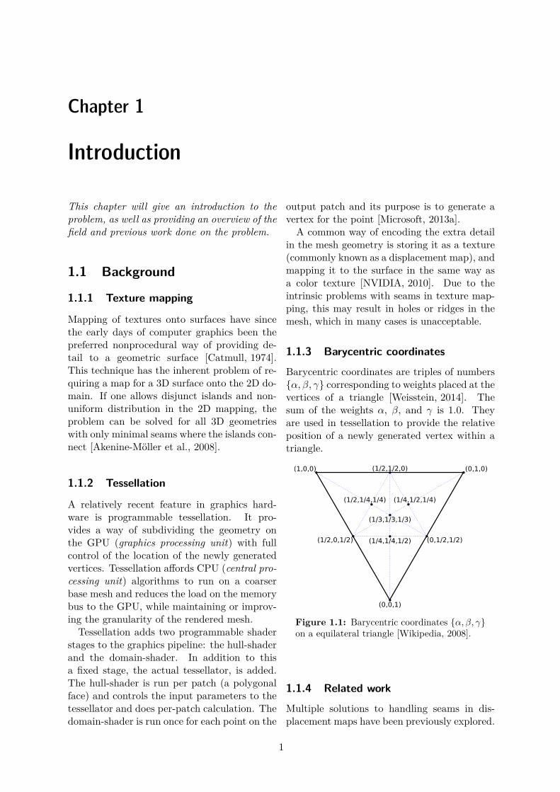
1.1.3 Barycentric coordinates

Barycentric coordinates are triples of numbers{α, β, γ} corresponding to weights placed at thevertices of a triangle [Weisstein, 2014]. Thesum of the weights α, β, and γ is 1.0. Theyare used in tessellation to provide the relativeposition of a newly generated vertex within atriangle.

Figure 1.1: Barycentric coordinates {α, β, γ}on a equilateral triangle [Wikipedia, 2008].

1.1.4 Related work

Multiple solutions to handling seams in dis-placement maps have been previously explored.

1

CHAPTER 1. INTRODUCTION

Piponi and Borshukov proposed a technique forfinding an optimal and intutive mapping called”pelting”, combined with a method for blendingtexture mappings together, to solve the prob-lem [Piponi and Borshukov, 2000]. Nießnerand Loop proposed a technique using a tiledtexture format and a displacement function,but it relies on a static topology and thusdoesn’t solve the issue of texture mapping adynamic topology [Nießner and Loop, 2013].

Sander et al. proposed a solution to tex-ture mapping progressive meshes by using tex-ture atlases, which solves some of the texturestretch issues, but not the problem with dy-namic topologies [Sander et al., 2001].

Yuksel et al. proposed a way of stor-ing surface color details directly associatedwith the 3D geometry surface, avoiding en-tirely the problem of mapping between tex-ture and model space [Yuksel et al., 2010].Schäfer et al. later extended this, proposinga similar technique for handling displacementdata [Schäfer et al., 2012]. Both these methodsprovide a one to one mapping between surfacedata and topology, and are thus feasable to useon dynamic topologies. We will further explorethe techniques presented in these papers in thisthesis.

1.2 Problem definition

In this thesis we will go through the pro-cess of implementing and combining the al-gorithm by Yuksel et al. with the algorithmby Schäfer et al. to provide a technique thatis completely free from texture mapping whilestill providing both color and geometry de-tails [Yuksel et al., 2010] [Schäfer et al., 2012].The original papers lack important details re-quired to implement the algorithms. We willprovide the details of our implementation here.

Schäfer et al. proposed in their ”Lim-itations and Future Work” section that ifthe hardware tessellator could provide aunique index per generated vertex, thecostly index retrieval algorithm could be re-moved [Schäfer et al., 2012]. We have experi-mented with removing the index retrieval al-gorithm by taking advantage of the hardwareavailable today, namely Compute Shaders, that

can perform general purpose computing onGPUs (GPGPU). This also eliminates anotherlimitation mentioned by Schäfer et. al in ”Lim-itations and Future Work”, that current hard-ware only supports tessellation factors up to64. It may also increase performance on AMDhardware where tessellation performance ingeneral is not on par with NVIDIA hardware,while usually outperforming NVIDIA hardwarewhen it comes to GPGPU (General PurposeGPU).

1.2.1 Limitations

We will not consider the problem of compress-ing the data on disk or the actual generation ofthe surface data. For testing purposes, we willconvert texture mapped surfaces to our dataformat, but we will not be concerned with cre-ating a signal optimal approach such as the oneused by H.Schäfer et al., since our primary pur-pose for the algorithm is to directly work withthe new data format, and not conversion fromexisting textures.

1.3 Purpose

The main purpose behind evaluating thesetechniques, beside the obvious advantageof eliminating discontinuities and distortionscaused by texture mapping, is the usage on adynamic topology.

Simulated or hand-crafted dynamic topologymesh morphing can be used to improve aes-thetics and realism. For these techniques tohave applications in games or other real-timesystems, a replacement for texture mapping isrequired. Animation of the texture mapping isinfeasible when it contains discontinuities, as isthe case in complex models.

Since these techniques stores the surface datadirectly related to the topology, moving trian-gles around on the surface does not require ad-ditional work to keep the surface data intact.Furthremore, adding geometry does not raisefurther challenges, given that the only requiredupdate is the insertion of the data for the newfaces.

A secondary advantage of these techniques isthat they could allow artist to directly paint on

2

1.4. PERFORMANCE MEASUREMENT

the mesh. This could be useful even if one endup baking the data to a traditional texture inthe end.

In addition to these advantages, these tech-niques could also be useful in the case ofprocedurally-generated meshes and other casesof programmatically processed meshes.

We have chosen to evaluate these techniquessince they have the potential to be used in real-time applications, and work well for dynamictopologies.

1.4 Performance measurementWe carry out all performance measurements inthis thesis using DirectX Queries with resultsin milliseconds. This metric provides the actualprocess time on the GPU.

3

Chapter 2

Implementation

Here we provide the details of the implementa-tion of the techniques, including problems andsolution for overcoming them.

2.1 The tessellator pattern

One of the main problems we faced implement-ing H.Schäfer’s multiresolution algorithm wasto imitate the hardware tessellator on the CPU.This is required to get the exact barycentriccoordinates for the vertices generated by thehardware tessellator. In turn, this precisionsupports the generation of correct surface dataand provides the base for our Compute Shaderimplementation of tessellation.

Unfortunately, Microsoft and the hardwareproviders are restrictive with the implementa-tion details of their tessellators, and the bestdescription found was the one provided by F.Giesen in ”A trip through the Graphics Pipeline2011, part 12: Tessellation” [Giesen, 2011].From Giesen we deduced the following method,which exactly imitates the hardware tessellatorfor even tessellation factors.

For edges, the tessellation is obvious; fora tessellation factor TE the edge is dividedinto TE equally large parts. For faces, on theother hand, the subdivision is less obvious; theface tessellation first divides the triangle intoa number of rings. For a tessellation factor Tthe number of rings are T

2 . For even tessella-tion factors the innermost ring is a degeneratetriangle.

Then, for each ring, the three corner verticesare calculated using θr, φr (equation (2.1)) (forring r where 1 ≤ r ≤ rings).

Figure 2.1: A triangle with tessellation level 4with two rings; one normal and one degeneratetriangle.

θr = 13

+ (23

∗ 1rings

)(rings − r)

φr = 1 − θr

2(2.1)

The three vertices {α, β, γ} building the in-ner triangle are:

αβγ

=

θr φr φr

φr θr φr

φr φr θr

(2.2)

That is, each corner vertex is built from oneprimary component ( θr ) and two smaller com-ponents ( φr ) of equal size. Since the barycen-tric coordinates must sum up to one, the twosmaller components are easily calculated fromthe primary one.

The primary component is calculated as thedistance in rings from the center of the triangle(1

3 , 13 , 1

3). The distance from an outer triangle

4

2.2. DISPLACEMENT SURFACE DATA

corner to the center is 23 (since the center is at

component value 13), and all rings are equally

spaced from each other, thus the formula forθr.

Each edge on the ring is then subdivided intoT − 2r equal big parts. The hardware tessella-tor takes the tessellation factors for the edgesin the order u == 0, v == 0, w == 0. That isin terms of our vertices β → γ, γ → α, α → β,so to ensure consistency we always process theedges in this order. Thus we generate thebarycentric coordinates for the vertices accord-ingly.

Figure 2.2: A triangle tessellated with tes-sellation level 4 on all edges and its face.

2.2 Displacement surface dataWe have implemented ”Multiresolution at-tributes for tessellated meshes” bySchäfer et. al. but limited to triangle primi-tives [Schäfer et al., 2012]. The technique gen-erates data for the same positions generated bythe hardware tessellator, thus eliminating theneed for filtering the data.

Since the fixed GPU tessellator only outputsthe barycentric coordinates for the generatedvertices, the first step of the domain shaderis to convert these coordinates into somethingmore useful. Schäfer et. al proposes the useof a ring-, edge- and vertex-index (hencefor-ward known as REV), since these are relativelypainless to calculate from the barycentric co-ordinates. This conversion is well covered by

H.Schäfer et al. and is thus not repeated here.The REV coordinates are each relative to theircurrent scope, that is ring to the current face,edge to the current ring, and vertex to the cur-rent edge.

2.2.1 On face index given REV

The next step is to find the location in the pointdata buffer for the current REV. For outeredges and the three original vertices this is astraightforward usage of the V-index (for outeredges) or E-index (for original vertices), butthe vertices on the face requires a bit more at-tention. Moreover, the original paper lacks thedetails of this implementation.

From the V-formula in the original paper(equation (2.3)), we can deduce that the num-ber of indices on any edge on ring R is (T −2R),giving the formula in equation (2.4) for thenumber of indices on a ring R (T is the tes-sellation factor, in this case the inner).

V = b′E

α + β + γ − 3bmin(T − 2R) (2.3)

indices(R) = 3(T − 2R) (2.4)

The unique index relative to the face for anyvertex is then the number of vertices in all theprevious rings (starting at R1, since R0 is theedge ring) plus the number of vertices in allthe previous edges on the current ring, plus thecurrent vertex index (equation (2.5)).

I(R, E, V ) =R−1∑r=1

indices(r) (2.5)

+ E(T − 2R) + V

By using the formula for the sum ofan arithmetic progresssion, followed by re-duction this can be simplified to equa-tion (2.6) [Wikipedia, 2014a].

I(R, E, V ) = 3(R − 1)(T − R) (2.6)+E(T − 2R) + V

5

CHAPTER 2. IMPLEMENTATION

Precalculating the data for the pointbuffer

Next, we need to have the actual displacementdata in the point buffer. For this, we calculatethe barycentric coordinates for all vertices withthe method described in section 2.1. These val-ues are sent to an algorithm generating data forthat position, either through texture lookup orsome procedural algorithm.

We precompute and store the new normalsfor the vertex. Care should be taken when ren-dering to use the original normal when apply-ing the displacement, and not the generatedone. Since generating the data takes time forcomplex meshes, we generate and store it in asimple file structure in a preprocess step.

2.3 Mesh colorsThe original paper explains in detail the meshcoloring algorithm [Yuksel et al., 2010]. Thus,we will not describe it here. The paper doesnot provide implementation details surround-ing the index lookup given the coordinate Bij

(figure 2.3) (from section 4.1 ”2D Filtering”).Those details we will describe here.

2.3.1 Index calculationStarting with Bij , we have three cases; vertex,edge, or face. If Bij exactly matches one vertexcoordinate we are on a vertex. If either of Bi

or Bj are zero, or the sum of the two is equalto the resolution R, we are on an edge. In allother cases we are on the face.

The formulas for calculating the indices andoffset in the data buffer are given in the sectionsbelow.

Vertex

Vindex =

0 if Bj = R

1 if Bi = 0 and Bj = 02 if Bi = R

(2.7)

Edge

Eindex =

0 if Bi = 01 if Bj = 02 if Bi = 0 and Bj = 0

(2.8)

Figure 2.3: The coordinate Bij for the ver-tices of a triangle.

Eoffset =

R − Bj if Eindex = 0Bi if Eindex = 1Bj if Eindex = 2

(2.9)

Face

For faces, the data offset is the sum of all theprevious columns plus the row offset. The rowand column indices both start at one, since in-dex 0 is contained within the edges.

Foffset =i−1∑k=1

(R − (k + 1)) + (j − 1)

=(2R − 2 − i) ∗ (i − 1)2

+ (j − 1)

(2.10)

2.3.2 Differences in ourimplementation

Given the improvements in hardware since theoriginal paper, we have used a structured arraybuffer instead of using the original workaroundswith 2D textures [Yuksel et al., 2010]. We alsocombine the data lookup with the displacementlookup. We must still use per vertex data inthe fragment shader, but we can use integerswithout interpolation between stages, a featurethat was not widely available in 2010 hardware.

6

2.4. LOD-LEVELS AND MIP-MAPPING

2.4 LOD-levels andMIP-mapping

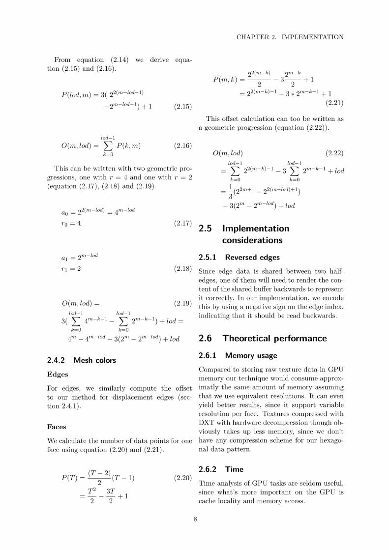
We have support for storing and rendering dif-ferent LOD and MIP-level, but the selectionof which level to use is outside of the scope ofthis thesis, and thus in our implementation theselection is done manually for the whole mesh.

For both displacement and color data, wepregenerate m = log2(T ) LOD-levels (for col-ors this is equivalent to MIP-levels). We storethe LOD-levels contiguously in memory. Thedata for a given LOD-level can be accessed byadding an offset to the list’s header memoryaddress.

Note that LOD-level 0 is the highest resolu-tion, and LOD-level m has lowest resolution.The tessellation factor T for a LOD-level lod(and equivalently resolution for mesh colors) isT = 2m−lod.

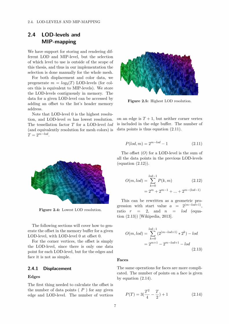
Figure 2.4: Lowest LOD resolution.

The following sections will cover how to gen-erate the offset in the memory buffer for a givenLOD-level, with LOD-level 0 at offset 0.

For the corner vertices, the offset is simplythe LOD-level, since there is only one datapoint for each LOD-level, but for the edges andface it is not as simple.

2.4.1 Displacement

Edges

The first thing needed to calculate the offset isthe number of data points ( P ) for any givenedge and LOD-level. The number of vertices

Figure 2.5: Highest LOD resolution.

on an edge is T + 1, but neither corner vertexis included in the edge buffer. The number ofdata points is thus equation (2.11).

P (lod, m) = 2m−lod − 1 (2.11)

The offset (O) for a LOD-level is the sum ofall the data points in the previous LOD-levels(equation (2.12)).

O(m, lod) =lod−1∑k=0

P (k, m) (2.12)

= 2m + 2m−1 + ... + 2m−(lod−1)

This can be rewritten as a geometric pro-gression with start value a = 2(m−lod+1),ratio r = 2, and n = lod (equa-tion (2.13)) [Wikipedia, 2013].

O(m, lod) =lod−1∑k=0

(2(m−lod+1) ∗ 2k) − lod

= 2m+1 − 2m−lod+1 − lod(2.13)

Faces

The same operations for faces are more compli-cated. The number of points on a face is givenby equation (2.14).

P (T ) = 3(T 2

4− T

2) + 1 (2.14)

7

CHAPTER 2. IMPLEMENTATION

From equation (2.14) we derive equa-tion (2.15) and (2.16).

P (lod, m) = 3( 22(m−lod−1)

−2m−lod−1) + 1 (2.15)

O(m, lod) =lod−1∑k=0

P (k, m) (2.16)

This can be written with two geometric pro-gressions, one with r = 4 and one with r = 2(equation (2.17), (2.18) and (2.19).

a0 = 22(m−lod) = 4m−lod

r0 = 4 (2.17)

a1 = 2m−lod

r1 = 2 (2.18)

O(m, lod) = (2.19)

3(lod−1∑k=0

4m−k−1 −lod−1∑k=0

2m−k−1) + lod =

4m − 4m−lod − 3(2m − 2m−lod) + lod

2.4.2 Mesh colors

Edges

For edges, we similarly compute the offsetto our method for displacement edges (sec-tion 2.4.1).

Faces

We calculate the number of data points for oneface using equation (2.20) and (2.21).

P (T ) = (T − 2)2

(T − 1) (2.20)

= T 2

2− 3T

2+ 1

P (m, k) = 22(m−k)

2− 32m−k

2+ 1

= 22(m−k)−1 − 3 ∗ 2m−k−1 + 1(2.21)

This offset calculation can too be written asa geometric progression (equation (2.22)).

O(m, lod) (2.22)

=lod−1∑k=0

22(m−k)−1 − 3lod−1∑k=0

2m−k−1 + lod

= 13

(22m+1 − 22(m−lod)+1)

− 3(2m − 2m−lod) + lod

2.5 Implementationconsiderations

2.5.1 Reversed edges

Since edge data is shared between two half-edges, one of them will need to render the con-tent of the shared buffer backwards to representit correctly. In our implementation, we encodethis by using a negative sign on the edge index,indicating that it should be read backwards.

2.6 Theoretical performance

2.6.1 Memory usage

Compared to storing raw texture data in GPUmemory our technique would consume approx-imatly the same amount of memory assumingthat we use equivalent resolutions. It can evenyield better results, since it support variableresolution per face. Textures compressed withDXT with hardware decompression though ob-viously takes up less memory, since we don’thave any compression scheme for our hexago-nal data pattern.

2.6.2 Time

Time analysis of GPU tasks are seldom useful,since what’s more important on the GPU iscache locality and memory access.

8

2.7. COMPUTE SHADER TESSELLATION

2.7 Compute shader tessellationWe have implemented a version of the integersubdivision tessellation pattern in a computeshader. The primary reason for this was to seeif performance could be improved by having thetessellator yield a unique index instead of onlya barycentric coordinate. To contain complex-ity, our implementation is limited to work onlywith even integer tessellation factors.

2.7.1 Buffer size calculationSince compute shaders is unable to allocateglobal memory or issue draw calls a bufferto store all the generated vertices and indicesmust be generated before the compute shadercan run. Thus, we need to know the exact num-ber of vertices and indices that would be gen-erated.

For inner tessellation, given the factor T thenumber of vertices is equation (2.25).

nV (R) = 3(R − 1)(T − R) + 1 (2.23)

nR(T ) = 32

T · 13

= T

2(2.24)

nV (T ) = 3(T

2− 1)(T − T

2) + 1

= 3(T 2

4− T

2) + 1 (2.25)

The reason for the single +1 in the formulais that the innermost triangle is a degeneratetriangle (single vertex) for even tessellation fac-tors (which is the only one we support).

The number of edge segments are the numberof vertices without the last degenerate triangle.Thus:

nE(T ) = nV (T ) − 1 = 3(T 2

4− T

2) (2.26)

The number of faces are twice the number ofedges, since for each edge segment one triangleis added outwards, and one inwards:

nF (T ) = 2 ∗ nE(T ) = 6(T 2

4− T

2) (2.27)

For the outer edges, these numbers are sim-ply the edge tessellation factor (both for num-ber of vertices and number of faces).

For triangle list rendering, the number of in-dices are three times the number of faces. Theactual number of indices drawn is controlledby an indirect draw call to support controllingLOD-levels from the GPU.

2.7.2 Triangle pattern generationGeneration of the vertices follow the methoddescribed in section 2.1. We then need to con-nect them by generating indices. In this sec-tion, we will cover the method for generatingthem for triangle lists, but in the optimizationsection we will show how to calculate indicesfor triangle strips.

Each ring on the face is processed separatelyand, since the edges are special, they are han-dled separately from the inner rings. For eachline segment on the ring, a face is generatedconnecting inwards. For the inner segments,another face is added connecting outwards.

Inwards connecting point

The first value needed to calculate the index forthe vertex on the next ring inwards is the ratiobetween the inner and outer ring, the ”trianglefactor” TF (equation (2.28)), where ES is thenumber of line segments on the inner and outeredge.

TF = ESI + 1ESO

(2.28)

IC = (ESI ∗ IE (2.29)+ ⌊TF ∗ (IV + 1)⌋) mod 3ESI

Equation (2.29) show how to calculate theconnect index inwards, where IE and IV is theindex of the edge and vertex relative to theircontext (ring and edge respectively). The for-mula is only valid for ESI > 0 since modulo 0is undefined. The index calculated is relativeto the inner ring.

Outwards connecting point

In the same way as we calculate the inwardsconnecting point, we need to calculate a point

9

CHAPTER 2. IMPLEMENTATION

for connecting the outwards face from the linesegment. These points must be selected so thatthe triangles do not overlap with the inwardsfaces, thus the triangle factor is the inverse ofthe triangle factor for the inwards face, and weround up instead of down.

TF = ESO

ESI + 1(2.30)

IC = ⌈TF ∗ (IV + 1)⌉ (2.31)

The index calculated in equation (2.31) is asopposed to the inwards index not relative tothe ring, but to the edge. This is due to thefact that for the outermost ring, the size of theedges are not consistent throughout the ringand needs to be handled separately. Care muststill be taken to be sure to keep the index insidethe ring, in the same way as the modulo in theinward case.

2.7.3 Per-face buffer offset

For each face we need to find where in thevertex and index buffer to start writing ourdata. We do this by keeping a buffer with thenext write offsets in and reserving the size ofthe current face (found by using the formulasdescribed in section 2.7.1) with atomic opera-tions.

The offset cannot be calculated per-face sincethe tessellation level may vary and, thus, asingle face cannot calculate the offset withoutknowing the previous faces’ tessellation factors.

2.8 Optimizations

Both of these optimizations are only applicableto the compute shader tessellator.

2.8.1 Data compression

The segment consuming the majority of thetime in the compute shader is the sequence ofwrites to global memory for indices and ver-tices. To reduce this, as many of the calcula-tions as possible is moved to the vertex shader.This reduces the amount of data needed to bewritten from the compute shader.

The data compression optimization that wehave accomplished stores the barycentric coor-dinate {α, β, γ} in one 32 bit integer by storingtwo of the components ( α, β ) as 16-bit in-tegers and calculating the last one from these( α + β + γ = 1 ).

2.8.2 Triangle strips

As writing to memory takes up the mayorpart of the tessellation and there are manymore indices than vertices, performance canbe increased by reducing the number of in-dices by using triangle strips instead of trianglelists [Microsoft, 2013b].

Index structure

How the indices are generated needs some carefor triangle strips so as to get winding orderright, connecting the different rings and evenmore so for connecting the different trianglesin the mesh (which may not be next to eachother). The special cases are handed using de-generate triangles which are not rendered.

When processing the original triangles westart and end each with double vertices, this tomake sure that they can always connect withthe next and previous triangle group and thatthere wont be any problems with the first andlast triangle in the mesh. Each ring inside thetriangle also starts and ends with double ver-tices. The double start vertices are the sameas the triangle start vertices for the outer edge.Figure 2.6 illustrates the double lines with tri-angle strips.

For each edge section, two indices are gen-erated (as opposed to the six indices generatedfor triangle lists). Of these indices, one is on thecurrent edge and one, on the next ring inwards.The formula for the inwards facing index is al-most the same as before (equation (2.32)).

IC = (ESI∗IE+⌊TF ∗(IV )⌋) mod 3ESI (2.32)

Number of indices

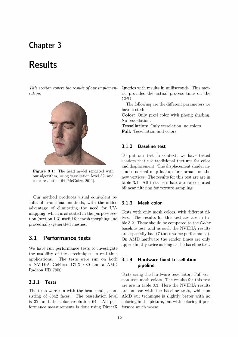
The number of indices have obviously changed.The new formulas for calculating the numberof indices are equation (2.33) and (2.34).

10

2.8. OPTIMIZATIONS

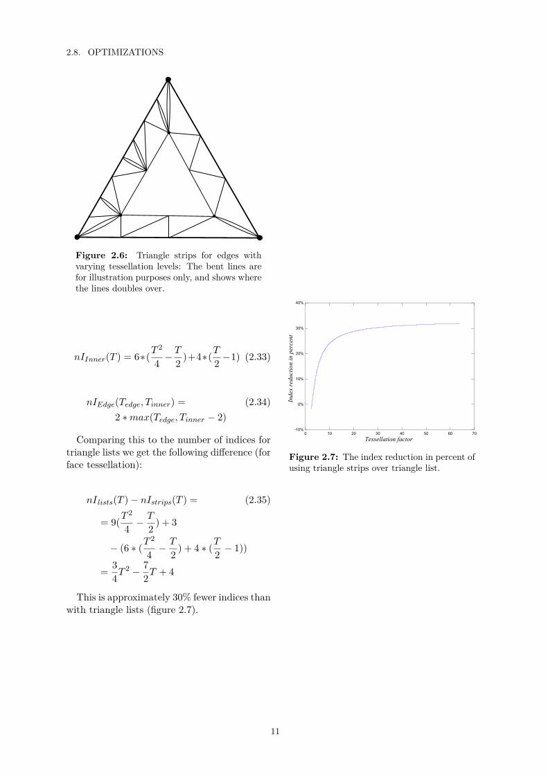
Figure 2.6: Triangle strips for edges withvarying tessellation levels: The bent lines arefor illustration purposes only, and shows wherethe lines doubles over.

nIInner(T ) = 6∗(T 2

4− T

2)+4∗(T

2−1) (2.33)

nIEdge(Tedge, Tinner) = (2.34)2 ∗ max(Tedge, Tinner − 2)

Comparing this to the number of indices fortriangle lists we get the following difference (forface tessellation):

nI lists(T ) − nIstrips(T ) = (2.35)

= 9(T 2

4− T

2) + 3

− (6 ∗ (T 2

4− T

2) + 4 ∗ (T

2− 1))

= 34

T 2 − 72

T + 4

This is approximately 30% fewer indices thanwith triangle lists (figure 2.7).

-10%

0%

10%

20%

30%

40%

0 10 20 30 40 50 60 70

Tessellation factor

Ind

ex r

edu

ctio

n i

n p

erce

nt

Figure 2.7: The index reduction in percent ofusing triangle strips over triangle list.

11

Chapter 3

Results

This section covers the results of our implemen-tation.

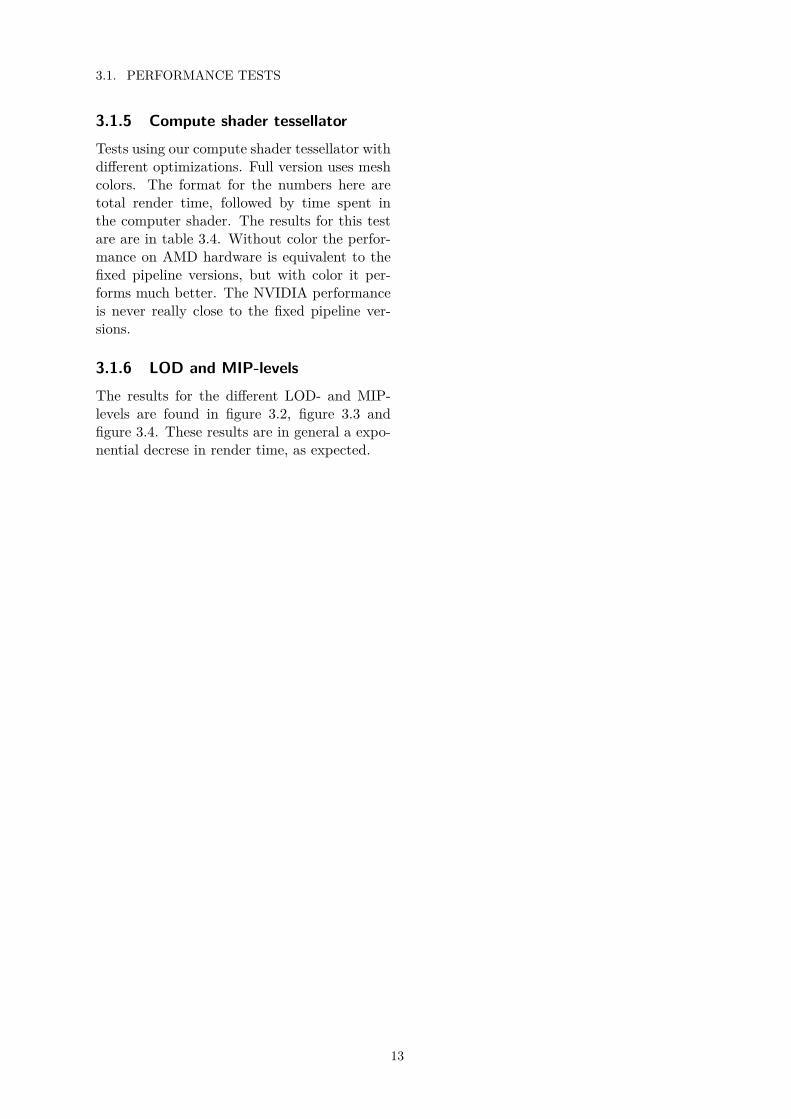
Figure 3.1: The head model rendered withour algorithm, using tessellation level 32, andcolor resolution 64 [McGuire, 2011].

Our method produces visual equivalent re-sults of traditional methods, with the addedadvantage of elimitating the need for UV-mapping, which is as stated in the purpose sec-tion (section 1.3) useful for mesh morphing andprocedually-generated meshes.

3.1 Performance testsWe have run performance tests to investigatethe usability of these techniques in real timeapplications. The tests were run on botha NVIDIA GeForce GTX 680 and a AMDRadeon HD 7950.

3.1.1 Tests

The tests were run with the head model, con-sisting of 8842 faces. The tessellation levelis 32, and the color resolution 64. All per-formance measurements is done using DirectX

Queries with results in milliseconds. This met-ric provides the actual process time on theGPU.

The following are the different parameters wehave tested:Color: Only pixel color with phong shading.No tessellation.Tessellation: Only tesselation, no colors.Full: Tessellation and colors.

3.1.2 Baseline test

To put our test in context, we have testedshaders that use traditional textures for colorand displacement. The displacement shader in-cludes normal map lookup for normals on thenew vertices. The results for this test are are intable 3.1. All tests uses hardware acceleratedbilinear filtering for texture sampling.

3.1.3 Mesh color

Tests with only mesh colors, with different fil-ters. The results for this test are are in ta-ble 3.2. These should be compared to the Colorbaseline test, and as such the NVIDIA resultsare especially bad (7 times worse performance).On AMD hardware the render times are onlyapproximatly twice as long as the baseline test.

3.1.4 Hardware-fixed tessellationpipeline

Tests using the hardware tessellator. Full ver-sion uses mesh colors. The results for this testare are in table 3.3. Here the NVIDIA resultsare on par with the baseline tests, while onAMD our technique is slightly better with nocoloring in the picture, but with coloring it per-formce much worse.

12

3.1. PERFORMANCE TESTS

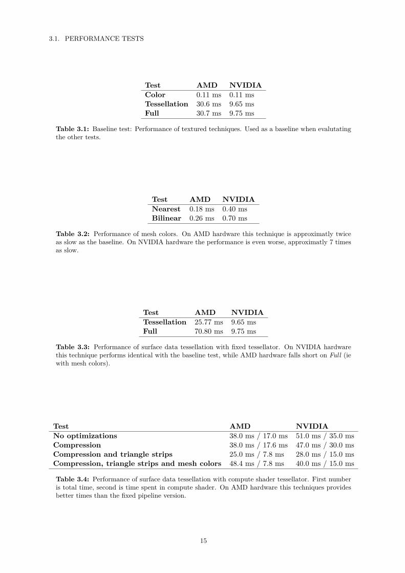
3.1.5 Compute shader tessellatorTests using our compute shader tessellator withdifferent optimizations. Full version uses meshcolors. The format for the numbers here aretotal render time, followed by time spent inthe computer shader. The results for this testare are in table 3.4. Without color the perfor-mance on AMD hardware is equivalent to thefixed pipeline versions, but with color it per-forms much better. The NVIDIA performanceis never really close to the fixed pipeline ver-sions.

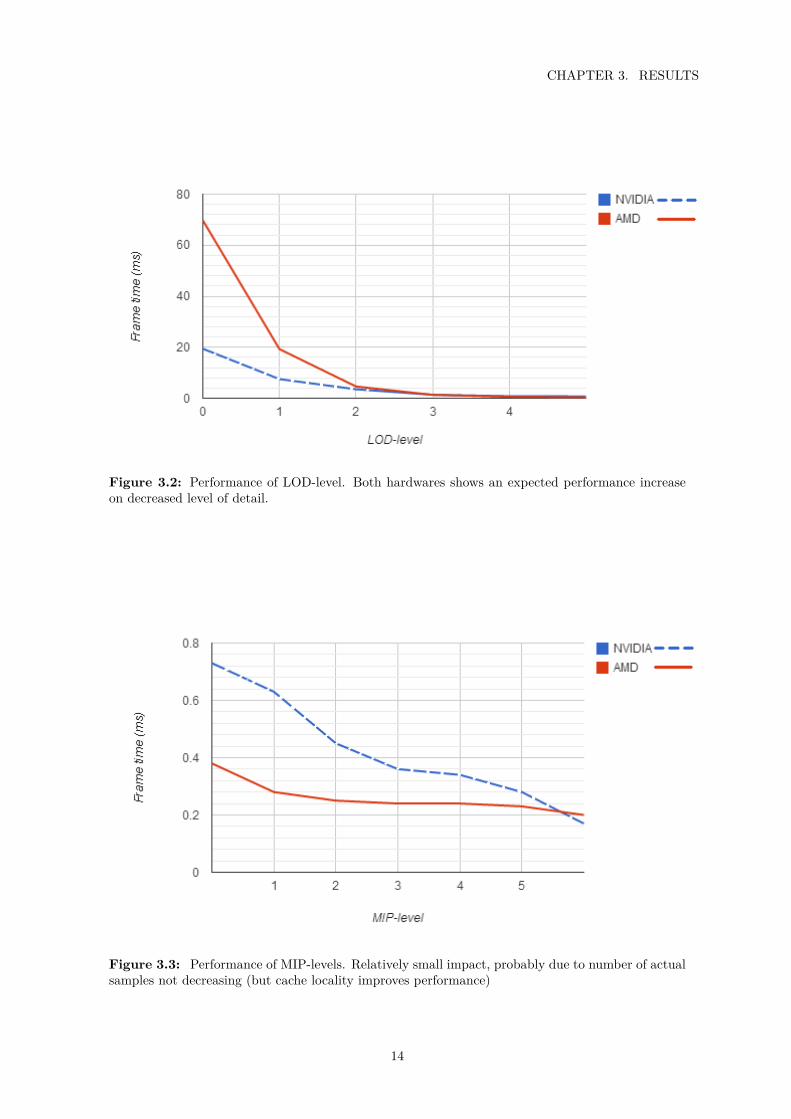
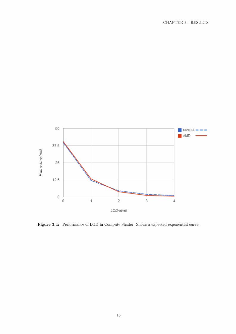
3.1.6 LOD and MIP-levelsThe results for the different LOD- and MIP-levels are found in figure 3.2, figure 3.3 andfigure 3.4. These results are in general a expo-nential decrese in render time, as expected.

13

CHAPTER 3. RESULTS

Figure 3.2: Performance of LOD-level. Both hardwares shows an expected performance increaseon decreased level of detail.

Figure 3.3: Performance of MIP-levels. Relatively small impact, probably due to number of actualsamples not decreasing (but cache locality improves performance)

14

3.1. PERFORMANCE TESTS

Test AMD NVIDIAColor 0.11 ms 0.11 msTessellation 30.6 ms 9.65 msFull 30.7 ms 9.75 ms

Table 3.1: Baseline test: Performance of textured techniques. Used as a baseline when evalutatingthe other tests.

Test AMD NVIDIANearest 0.18 ms 0.40 msBilinear 0.26 ms 0.70 ms

Table 3.2: Performance of mesh colors. On AMD hardware this technique is approximatly twiceas slow as the baseline. On NVIDIA hardware the performance is even worse, approximatly 7 timesas slow.

Test AMD NVIDIATessellation 25.77 ms 9.65 msFull 70.80 ms 9.75 ms

Table 3.3: Performance of surface data tessellation with fixed tessellator. On NVIDIA hardwarethis technique performs identical with the baseline test, while AMD hardware falls short on Full (iewith mesh colors).

Test AMD NVIDIANo optimizations 38.0 ms / 17.0 ms 51.0 ms / 35.0 msCompression 38.0 ms / 17.6 ms 47.0 ms / 30.0 msCompression and triangle strips 25.0 ms / 7.8 ms 28.0 ms / 15.0 msCompression, triangle strips and mesh colors 48.4 ms / 7.8 ms 40.0 ms / 15.0 ms

Table 3.4: Performance of surface data tessellation with compute shader tessellator. First numberis total time, second is time spent in compute shader. On AMD hardware this techniques providesbetter times than the fixed pipeline version.

15

CHAPTER 3. RESULTS

Figure 3.4: Performance of LOD in Compute Shader. Shows a expected exponential curve.

16

Chapter 4

Discussion

This section covers our reasoning surroundingthe results and the future possibilities for it.

4.1 AnalysisAs can be seen from the performance tests thehardware tessellator on AMD have some issues.Whats interesting though is how much worsethe AMD card performed in the full test versushow it performed in the tessellator only test,especially since the times for mesh colors aloneis in the context negligible. We have found thatthe cause for this performance hit is the extradata that needs to be sent from the domainshader to the vertex shader for mesh colors towork. AMD cards have issues with too muchdata being sent between shader stages. This isa good point for future optimizations.

On the other hand the AMD card outper-forms the NVIDIA card when it comes to com-pute shaders (this is especially clear if one lookat the compute shader times only, 7.8 ms onAMD versus 15.0 ms on NVIDIA), and thatmakes it possible for us to perform our tessel-lation there, for better results.

The other notable difference between thecards is in mesh colors where the AMD cardis better. The reason for this might bethe higher memory bandwidth of the HD7950since mesh colors require a lot of mem-ory lookups, especially for the bilinear fil-ter [HWCompare, 2012].

The performance improvement of reducingthe LOD-level is no surprise, the tessellationreduction is in power-of-twos and the resultsreflects this. For the MIP-levels the improve-ment of reducing the MIP-levels is not very big,but this is not the primary reason for MIP-mapping. The number of lookups are not re-duced either, since that is controlled by thenumber of rendered fragments. The reason for

the performance improvement is probably dueto better cache locatity of the samples.

Worth noticing on the overall performance isthat the mesh used in the tests have a high polycount and that an unnecessarily high tessella-tion level was used. The performance times forour algorithms should be considered in compar-ison with the baseline tests.

There are also the consideration of storingthe displacement data in a different patternthan that for colors. Doing so saves filter-ing since the storage pattern always exactlymatches that from the tessellator, but on theother hand this adds complexity to the imple-mentation, and if in the future compression isconcidered, two different schemes, or a schemethat works on both patterns must be deviced.Thus it could be worth using the mesh colorpattern for both data types.

4.2 Conclusion

We have implemented and evaluated tech-niques for storing color and displacement datadirectly in a 3D-topology. From the perfor-mance results one can conclude that thesemethods could be usable in a real application,but since they obviously do not outperformthe traditional methods they should only beused in cases where they are more suitable thanthe traditional methods or when the traditionalmethods is infeasible.

Even if the color data and displacement datais stored in a similar way they should still behandled separately, since the desired resolutionfor colors is often higher than the desired res-olution for displacement. It could though beworth concidering using the same pattern forboth displacement and colors, to save imple-mentation complexity.

17

CHAPTER 4. DISCUSSION

4.3 Future workTo work well with meshes with dynamic topol-ogy animation of the data is probably needed.Animation could probably be solved relativelyeasy, given that support for effectively stream-ing data to the GPU exists, but to properlyrender dynamic topology that would probablyalready be a requirement.

Another issue that needs to be addressed iscompression of the data, primary when storedon disk. One could also explore the possibil-ity to compress the color in the GPU meshcolor buffer to reduce the memory footprint.Another point of optimization is to reduce theamount of sent between shader stages for meshcolors, especially to improve performance onAMD cards.

18

Bibliography

[Akenine-Moller et al., 2008] Akenine-Moller,T., Haines, E., and Hoffman, N. (2008).Real-Time Rendering 3rd Edition, chapter6. Texturing, pages 147–199. A. K. Peters,Ltd., Natick, MA, USA.

[Catmull, 1974] Catmull, E. E. (1974). A Sub-division Algorithm for Computer Display ofCurved Surfaces. PhD thesis. AAI7504786.

[Giesen, 2011] Giesen, F. (2011). A tripthrough the graphics pipeline 2011, part 12.http://fgiesen.wordpress.com/2011/09/06/a-trip-through-the-graphics-pipeline-2011-part-12/. [Online; Ac-cessed 2013-10-10].

[HWCompare, 2012] HWCompare (2012).Geforce gtx 680 vs radeon hd 7950. http://www.hwcompare.com/12350/geforce-gtx-680-vs-radeon-hd-7950/. [Online;Accessed 2014-01-21].

[McGuire, 2011] McGuire, M. (2011). Com-puter graphics archive. http://graphics.cs.williams.edu/data. [Online; Accessed2014-01-21].

[Microsoft, 2013a] Microsoft (2013a). Tessel-lation overview. http://msdn.microsoft.com/en-us/library/windows/desktop/ff476340(v=vs.85).aspx. [Online; Ac-cessed 2014-01-21].

[Microsoft, 2013b] Microsoft (2013b). Tri-angle strips. http://msdn.microsoft.com/en-us/library/windows/desktop/bb206274(v=vs.85).aspx. [Online; Ac-cessed 2014-01-21].

[Nießner and Loop, 2013] Nießner, M. andLoop, C. (2013). Analytic displacementmapping using hardware tessellation. ACMTrans. Graph., 32(3):26:1–26:9.

[NVIDIA, 2010] NVIDIA (2010). Directx11 tessellation. http://www.nvidia.com/

object/tessellation.html. [Online; Ac-cessed 2014-01-21].

[Piponi and Borshukov, 2000] Piponi, D. andBorshukov, G. (2000). Seamless texturemapping of subdivision surfaces by modelpelting and texture blending. In Proceedingsof the 27th Annual Conference on ComputerGraphics and Interactive Techniques, SIG-GRAPH ’00, pages 471–478, New York, NY,USA. ACM Press/Addison-Wesley Publish-ing Co.

[Sander et al., 2001] Sander, P. V., Snyder, J.,Gortler, S. J., and Hoppe, H. (2001). Texturemapping progressive meshes. In Proceedingsof the 28th Annual Conference on ComputerGraphics and Interactive Techniques, SIG-GRAPH ’01, pages 409–416, New York, NY,USA. ACM.

[Schäfer et al., 2012] Schäfer, H., Prus, M.,Meyer, Q., Süßmuth, J., and Stamminger,M. (2012). Multiresolution attributes for tes-sellated meshes. In Proceedings of the ACMSIGGRAPH Symposium on Interactive 3DGraphics and Games, I3D ’12, pages 175–182, New York, NY, USA. ACM.

[Weisstein, 2014] Weisstein, E. W. (2014).Barycentric coordinates. [From MathWorld– A Wolfram Web Resource; Accessed 2014-01-24].

[Wikipedia, 2008] Wikipedia (2008).Triangle barycentric coordinates.http://en.wikipedia.org/wiki/File:TriangleBarycentricCoordinates.svg.[Online; Accessed 2014-02-08].

[Wikipedia, 2013] Wikipedia (2013). Geomet-ric progression. http://en.wikipedia.org/wiki/Geometric_progression. [On-line; Accessed 2014-01-21].

[Wikipedia, 2014a] Wikipedia (2014a). Arith-metic progression. http://en.wikipedia.

19

BIBLIOGRAPHY

org/wiki/Arithmetic_progression. [On-line; Accessed 2014-01-21].

[Wikipedia, 2014b] Wikipedia (2014b). Poly-gon mesh. http://en.wikipedia.org/wiki/Polygon_mesh. [Online; Accessed2014-12-28].

[Yuksel et al., 2010] Yuksel, C., Keyser, J.,and House, D. H. (2010). Mesh colors. ACMTrans. Graph., 29(2):15:1–15:11.

20

Appendix A

Glosary

• Barycentric coordinates A three com-ponent vector describing a position on atriangle (see section 1.1.3).

• Bilinear filtering A filtering techniquethat samples all neighboring pixels andsmoothly blends them.

• CPU Central Processing Unit

• DirectX A Graphics API on Microsoftsystems.

• DXT A texture compression algorithm fitfor real time decompression on the GPU

• GPU Graphics Processing Unit

• GPGPU General Purpose GPU. Refersto the ability to perform general comput-ing tasks on a GPU, often refered to aCompute Shaders.

• LOD Level of Detail. A sequence of ver-sions of the same mesh, with decreasingdetail.

• Mesh A collection of vertices edges andfaces that defines the shape of a three di-mensional solid with flat faces and sharpedges. [Wikipedia, 2014b].

• MIP Or Mipmaps. A pre-calculated opti-mized sequence of lower resolution versionsof a texture.

• Nearest filtering A filtering techniquethat always picks the color of the nearestneighboring pixel.

• REV Ring-, Edge-, Vertex-index.Acronym defined by H.Schäfer et al.refering to a three component vector ofindices describing a discrete position on atriangle.

• Tesselation The subdivision of a meshsurface into smaller triangles.

• Topology In the scope of this thesis thisrefers to the surface of a mesh.

• UV-mapping Or texture mapping. Themapping of a 2d dimensional texture ontothe surface of a 3d dimensional mesh.

21