Surface geometry determination by large-angle ion … · Surface geometry determination by large-angle ... physics and chemistry of solid surfaces has ... Surface geometry determination

Vacuum/volume 38/number Z/pages 129 to 142/l 988 0042-207X/8853.00 -I- .OQ

Printed in Great Britain Pergamon Press plc

Surface geometry determination by large-angle ion scattering Th Fauster. Max-Planck-lnstitut fiir Plasmaphysik, EURATOM Association, D-8046 Garching, FRG

received 18 June 1987

The current state of surface structure determination by ion scattering experiments at large scattering angles is reviewed.

1. Introduction

The rapidly increasing interest in the physics and chemistry of solid surfaces has been stimulated by the widespread use of technologies like catalysis and microelectronics which rely heavily on the properties of surfaces. Basic research on solid surfaces deals with the following three questions: (a) which elements are present on the surface? (b) what is the geometrical arrangement of the atoms on the surface? (c)what are the electronic properties of the surface? The separation of surface physics into these three problems is artificial since the answers to these questions are not independent from each other. For a given arrangement of a given number of elements the electronic structure is determined by quantum mechanics. The electronic forces, on the other hand, determine the geometrical structure and the surface composition by segregation, desorption or adsorption. An answer to one or two of the above questions, therefore, always gives information on the remaining questions. The subdivision of surface physics into three areas is done more for practical.reasons, since there are specific experiments answering the individual questions. The techniques for elemental analysis can be sensitive to the nuclear charge or the nuclear mass. The atomic number or nuclear charge is usually measured via excitation of core electrons and the most widely used techniques are Auger electron spectroscopy (AES) and X-ray photoelectron spectroscopy (XPS or ESCA)‘**. The nuclear mass can be measured by mass spectroscopy of sputtered particles (SIMS)3 or desorbed particles (TDS)4, or by scattering of ions or atoms off the surface (KS5 or RBS6). The determination of the surface geometry is possible by diffraction experiments- using photons (surface X-ray scattering)‘, electrons (LEED)8,9 or

atoms at thermal energies lo The energy of the probing particle is always adjusted to match the de-Broglie wavelength with typical atomic distances. The surface structure in real space can be determined by high resolution electron microscopy”, scanning tunnelling microscopy (STM)“, and ion scattering spectroscopy’3. All these techniques capable of measuring the static structure of a surface can, of course, also yield information on the dynamical behaviour of the surface atoms. The observation of surface phonons is possible by inelastic scattering of He atomsL4 or low energy electrons (HREELS)“. The determination

of the electronic structure always involves electronic transitions. The most powerful techniques in this area are ultraviolet photoelectron spectroscopy (UPS)16 and its complement inverse photoemission (IPE) . “.I8 We are going to concentrate in this review on structure determination by large-angle ion scattering and, therefore, we refer the reader to the textbooks’.” and reviews for more detailed information on the various techniques.

2. Scattering of low-energy ions

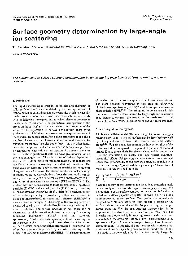
2.1. Binary collision model. The scattering of ions with energies ranging from 0.1 to 10 keV off surfaces can be described very well by binary collisions between the incident ion and surface atoms5.20-22. This is justified because the interaction time of the collisions is short compared to the period of phonons of the solid targets. Due to the small de-Broglie wavelength of the ion, we can treat the interaction classically and can neglect quantum- mechanical effects. Using energy and momentum conservation, it is then straightforwardly shown that the energy E, of an ion with mass ml and energy E, scattered through an angle 9 by an atom of mass m2 is given by (see Figure 1):

El ( cos9+ m,2/mf--sin2 9 2 -_= Gl 1 + m2/ml ).

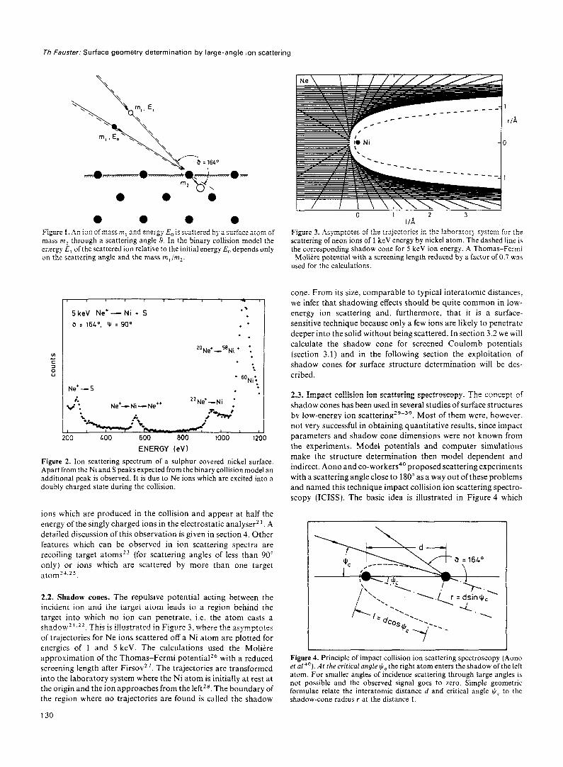
Since the energy of the scattered ion for a fixed scattering angle depends only on the mass ratio m,/m,, an energy spectrum gives a direct picture of the surface composition. An example for the so- called ion scattering spectroscopy (KS) is given in Figure 2 for a sulphur-covered nickel surface. Two peaks are immediately assigned to “Ne ions scattered from Ni and S atoms on the surface, where the shoulder of the Ni peak at higher energies comes from the 60Ni isotope. Another isotope effect is the appearance of a structure due to scattering of “Ne ions. The intensity ratio observed is in good agreement with the natural abundancy of these two Ne isotopes of 1: 9. The fourth peak of the spectrum in Figure 2 cannot be assigned to any plausible surface contamination. Its intensity did not change with surface preparation and no corresponding peak could be found with He ions. This leads to the conclusion that it arises from doubly charged Ne

129

Th Fauster: Surface geometry determination by large-angle ion scattering

\ \

\ \ \ A \ ml ’ 5 \ \ \ \ \

E’ \

m,, 0 -\ \

0 0 0 l Figure 1. An ion of mass m, and energy E,, is scattered by a surface atom of mass mz through a scattering angle 9. In the binary collision model the energy E, of the scattered ion relative to the initial energy E0 depends only on the scattering angle and the mass ml/mz

5keV Ne’-Ni + S

9 = 16L". W :90°

* . 20Ne+_5ENi. :

. . .

Ne*-S

t * 6oNi:

: . . .

Ne*- Ni -- Ne*+ 22Ne*-Ni *

.

c IO coo 600 000 1000 12(

ENERGY (eV)

Figure 2. Ion scattering spectrum of a sulphur covered nickel surface. Apart from the Ni and S peaks expected from the binary collision model an additional peak is observed. It is due to Ne ions which are excited into a doubly charged state during the collision.

ions which are produced in the collision and appear at half the energy of the singly charged ions in the electrostatic analyser’ I. A detailed discussion of this observation is given in section 4. Other

features which can be observed in ion scattering spectra are recoiling target atoms 23 (for scattering angles of less than 90”

only) or ions which are scattered by more than one target atom’4.25.

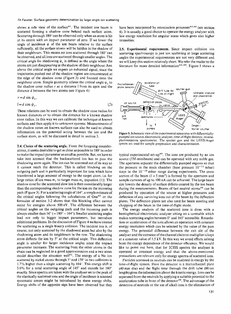
2.2. Shadow cones. The repulsive potential acting between the incident ion and the target atom leads to a region behind the target into which no ion can penetrate, i.e. the atom casts a shadow2’.22. This is illustrated in Figure 3, where the asymptotes of trajectories for Ne ions scattered off a Ni atom are plotted for energies of 1 and 5 keV. The calculations used the Moliere approximation of the Thomas-Fermi potential26 with a reduced screening length after Firsov 27 The trajectories are transformed into the laboratory system where the Ni atom is initially at rest at the origin and the ion approaches from the left”. The boundary of the region where no trajectories are found is called the shadow

130

1 _-- --

r/A

(/A

Figure 3. Asymptotes of the trajectories in the laboratory system for the scattering of neon ions of 1 keV energy by nickel atom. The dashed line is the corresponding shadow cone for 5 keV ion energy. A Thomas-Fermi -Moliere potential with a screening length reduced by a factor of 0.7 was used for the calculations.

cone. From its size, comparable to typical interatomic distances, we infer that shadowing effects should be quite common in low- energy ion scattering and, furthermore, that it is a surface- sensitive technique because only a few ions are likely to penetrate deeper into the solid without being scattered. In section 3.2 we will calculate the shadow cone for screened Coulomb potentials (section 3.1) and in the following section the exploitation of shadow cones for surface structure determination will be des-

cribed.

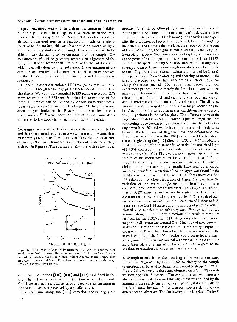
2.3. Impact collision ion scattering spectroscopy. The concept of shadow cones has been used in several studies ofsurface structures by low-energy ion scattering 29-39 Most of them were, however, not very successful in obtaining quantitative results, since impact parameters and shadow cone dimensions were not known from the experiments. Model potentials and computer simulations make the structure determination then model dependent and indirect. Aono and co-workers4’ proposed scattering experiments with a scattering angle close to 180” as a way out of these problems and named this technique impact collision ion scattering spectroscopy (ICISS). The basic idea is illustrated in Figure 4 which

Figure 4. Principle of impact collision ion scattering spectroscopy (Aono et a/““). At the critical angle $, the right atom enters the shadow of the left atom. For smaller angles of incidence scattering through large angles is not possible and the observed signal goes to zero. Simple geometric formulae relate the interatomic distance d and critical angle $, to the shadow-cone radius r at the distance I.


shows a side view of the surface4’. The incident ion beam is scattered forming a shadow cone behind each surface atom. Scattering through 180” can be observed only when an atom is hit at its centre with an impact parameter of zero. If we lower the angle of incidence I(/ of the ion beam relative to the surface sufficiently, all the surface atoms will be hidden in the shadow of their neighbours. This means no ions scattered through 180” can be observed, and ali ions are scattered through smaller angles. The critical angle for shadowing $, is defined as the angle where the atoms are just disappearing in the shadow of their neighbour. Just above the critical angle we expect an enhanced signal, since the trajectories pushed out of the shadow region are concentrated at the edge of the shadow cone (Figure 3) and focused onto the neighbour atom. Simple geometry relates the critical angle II/, to the shadow cone radius r at a distance I from its apex and the distance d between the two atoms (see Figure 4):

r=d sin $,,

l=d cos $,. (2)

These relations can be used to obtain the shadow cone radius for known distances or to obtain the distance for a known shadow cone radius. In this way we can calibrate the technique at known

surfaces and then apply it to unknown systems. Measurements of the shadow cones on known surfaces can also be used to obtain information on the potential acting between the ion and the surface atom, as will be discussed in detail in section 3.

2.4. Choice of the scattering angle. From the foregoing consider- ations, it seems desirable to get as close as possible to 180” in order to make the impact parameter as small as possible. But, we have to take into account that the backscattered ion has to pass the shadowing atom again. The ion can be scattered out of its way so it cannot reach the detector. This is called blocking on the outgoing path and is particularly important for ions which have transferred a large amount of energy to the target atom, i.e. for large ratios of ion mass M, to target mass m, (equation (1)). The shadow cone for the scattered slow ion is then considerably larger than the corresponding shadow cone for the ion on the incoming path (Figure 3). For a scattering angle of 164”, a simple estimate of the critical angles following the calculations of Oen4’ or the formulae of section 3.2 shows that this blocking effect cannot occur for energies above 500 eV. The difference between the critical angles on the outgoing path and the incoming path is always smaller than 16” (= 180” - 164”). Smaller scattering angles lead not only to bigger impact parameters, but introduce additional problems. In the discussion of Figure 4 we have treated the scattering as a single binary collision. The incident ion is, of course, not only scattered by the shadowed atom but also by the shadowing atom and its neighbours in the row. The shadowing atom deflects the ion by 5” at the critical angle. This deflection angle is smaller for larger incidence angles since the impact parameter increases. The scattering from the other atoms in the chain can be neglected to a good approximation and a two atom model describes the situation we114’. The energy of a Ne ion scattered by nickel atoms through 5” and 159” in two collisions is 1.7% higher than a single scattering by 164’. This energy shift is 3.6% for a total scattering angle of 145” and cancels for 180” exactly. Since spectra are taken with the analyser set to the peak of the elastically scattered ions and the angle of incidence is scanned systematic errors might be introduced by these energy shifts. Energy shifts of the opposite sign have been observed but they

have been interpreted by reionization processes43.44 (see section

4). It is usually a good choice to operate the energy analyser with low energy resolution for angular scans which gives also higher intensities.

2.5. Experimental requirements. Since impact collision ion scattering spectroscopy is just ion scattering at large scattering angles the experimental requirements are not very different and we will keep this section relatively short. We refer the reader to the literature for more detailed information45-48. Figure 5 shows a

drift lube for sputhY gun

rotatable onolyzer

ion Source

pumps V Muller counter

Figure 5. Schematic view of the experimental apparatus with differentially- pumped ion source, electrostatic analyser, time-of-flight detector, inverse- photoemission spectrometer. The sputter gun and the LEED/Auger system are used for sample preparation and characterization.

typical experimental set-up49. The ions are produced by an ion source (3M-minibeam) and can be operated with any noble gas. The apertures separate the differentially pumped regions so that the pressure in the main chamber (base pressure lo-” mbar) stays in the lo-” mbar range during experiments. The cross

section of the beam (1 x 5 mm2) is formed by the apertures and sample currents of up to 100 nA can be achieved. The large beam size lowers the density of surface defects created by the ion beam during the measurements. Beams of fast neutral atomss4 can be produced by operation of the source at higher pressures and deflection of any surviving ions out of the beam by the deflection plates. The deflection plates are also used for beam steering and chopping of the beam in the time-of-flight mode.

The energy analysis of the scattered ions is done with a hemispherical electrostatic analyser sitting on a turntable which makes scattering angles between 0” and 165” accessible. Retarda- tion or acceleration of the ions allows an operation with constant energy resolution which can be selected by the value of the pass energy. The potential difference between the exit slit of the analyser and the entrance of the channel electron multiplier is kept at a constant value of 1.5 kV. In this way we avoid effects arising from the energy dependence of the detector efficiency. We would

like to point out here, that for ICISS spectra the analyser is operated at constant energy and that the above-mentioned precautions are relevant only for energy spectra of scattered ions.

Particles scattered as neutrals can be analysed in energy by the time-of-flight system. Here the detector is a microchannel plate (40 mm dia) and the flight time through the drift tube (60 cm length) gives the information about the kinetic energy. Ions can be separated from the neutrals by applying a suitable potential to the acceleration tube in front of the detector”. The advantage of the detection of neutrals or the use of alkali ions is the elimination of

131

Th Fausfer: Surface geometry determination by large-angle ion scattering

the problems associated with the high neutralization probability of noble gas ions. These aspects have been discussed with reference to ICISS by Niehus51. Since ICISS spectra record the elastically scattered ions as a function of incidence angle IJ (relative to the surface) this variable should be controlled by a motorized rotary motion feedthrough. It is also essential to be able to vary the azimuthal orientation 47 of the sample. The measurement of surface geometry requires an alignment of the sample surface to better than 0.5’ relative to the rotation axes which is usually done by laser reflection. The orientation of the crystal planes relative to the geometrical surface can be checked by the ICISS method itself very easily, as will be shown in section 2.7.

For sample characterization a LEED/Auger system’ is shown in Figure 5, though we usually prefer ISS to monitor the surface cleanliness. We also find azimuthal ICISS scans (see section 2.7) more accurate than LEED for the azimuthal orientation of the samples. Samples can be cleaned by Ar ion sputtering from a separate ion gun and by heating. The Geiger-Miiller counter and electron gun indicated in Figure 5 are used for inverse photoemission’7.18 which permits studies of the electronic states in parallel to the geometric structure on the’same sample.

2.6. Angular scans. After the discussion of the concepts of ICISS and the experimental requirements we will present now some data which verify those ideas. The intensity of 5 keV Ne’ ions scattered elastically off a Cu(ll0) surface as a function of incidence angle $ is shown in Figure 6. The spectra are taken in the three low-index

I I 1 I I 1 I I

5 keV Ne’ -Cu (110). 9 :16L”

. [Ii01 . [Ii21 .

_-rj k I0011

00 300 60° 90°

ANGLE OF INCIDENCE ‘4

J

Figure 6. The number of elastically scattered Ne+ ions as a function of incidence angle IJ~ for threedifferent azimuths ofa Cu( 110) surface. The top view of the surface is shown in the inset, where the smaller circle represents an atom in the second layer. Third layer atoms are hidden by the large circles of the first layer atoms.

azimuthal orientations [liO], [OOI] and [IT23 as defined in the inset which shows a top view of the (110) surface of a fee crystal. First-layer atoms are shown as large circles, whereas an atom in the second layer is represented by a smaller circle.

The spectrum along the [liO] direction shows negligible

132

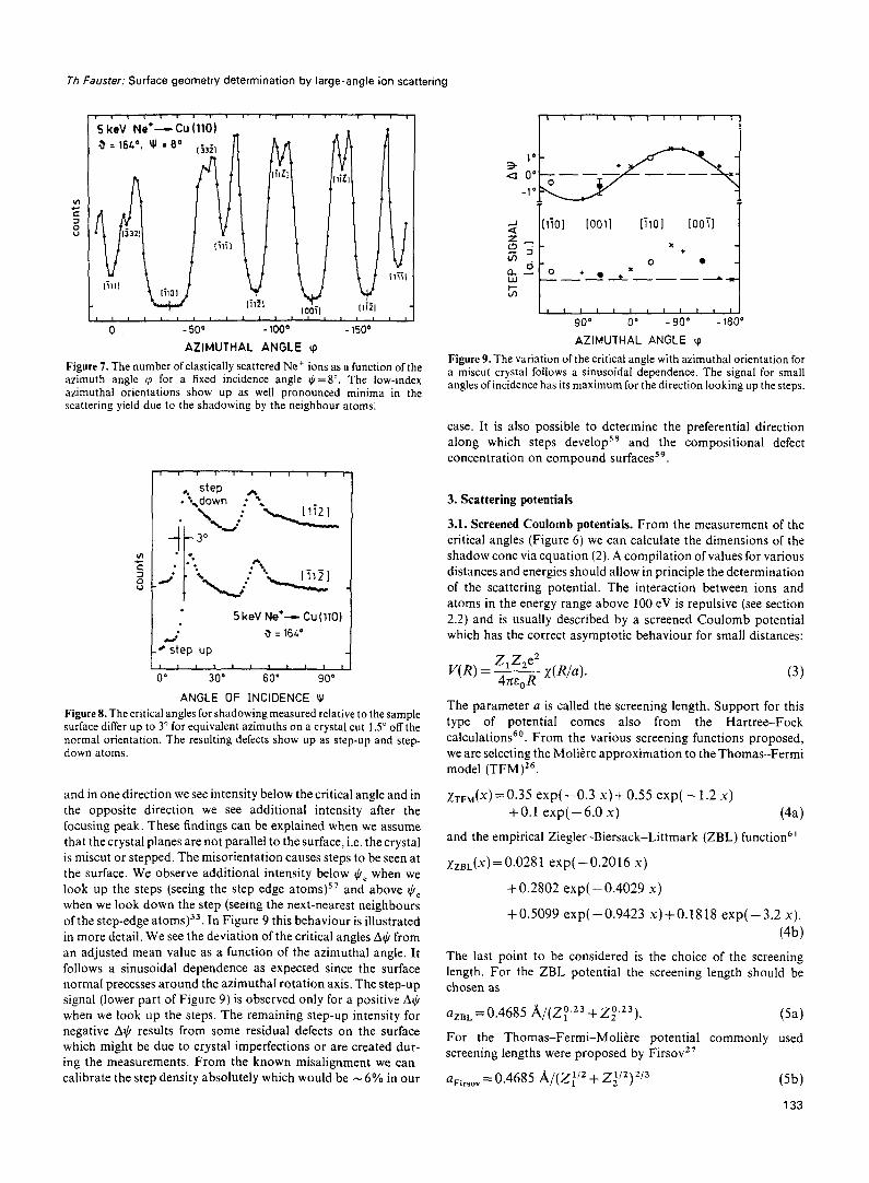
intensity for small 1+9, followed by a steep increase in intensity. After a pronounced maximum, the intensity of backscattered ions stays essentially constant. This is exactly the behaviour we expect after the discussion of Figure 4 in section 2.3. For small angles of incidence, all the atoms in the first layer are shadowed. At the edge of the shadow cone, the signal is enhanced due to focusing and levels off for larger $. We define the critical angle $, for shadowing at the point of half the peak intensity. For the [OOl] and [li2] azimuth, the spectra in Figure 6 show smaller critical angles 3, corresponding to larger nearest-neighbour distances. In contrast to the [ IiO] direction, a second maximum is observed for large $. This peak results from shadowing and focusing of atoms in the third and second layer by first layer atoms which cannot occur along the close packed [liO] rows. This shows that our experiment probes approximately the first three layers with the main contributions coming from the first layer5’. From the critical angles of the third- and second-layer shadowing we can deduce information about the surface relaxation. The distance between the shadowing atom and the second-layer atom along the [ 1 i2] azimuth is the same as the nearest-neighbour distance along the [ liO] azimuth in the surface plane. The difference between the two critical angles is 27.510.7” which is just the angle the lines connecting the two atom pairs enclose. For an ideal fee lattice this angle would be 30” and we deduce a contraction of the distance between the top layers of 10*3%. From the difference of the third-layer critical angle in the [OOl] azimuth and the first-layer critical angle along the [Ii?] direction of 35.OkO.7’ we obtain a small contraction of the distance between the first and third layer of I f 3%, corresponding to an expanded distance between layers two and three (8 k 6%). These values are in agreement with other studies of the oscillatory relaxation of (110) surfaces53,51 and support the validity of the shadow cone model and its transfer- ability to other systems. Similar results have been obtained for nickel surfacess9~55. Relaxation of the top layers was found for the (110) surface, whereas the (001) and (111) surfaces show less than 1% relaxation. A close inspection of Figure 6 shows that the variation of the critical angle for the different azimuths is comparable to the steepness of the onsets. This suggests a different type of ICISS measurement, where the angle of incidence is kept constant and the azimuthal angle cp is varied56. The result of such an experiment is shown in Figure 7. The angle of incidence is 8- relative to the Cu( 110) surface and the number of scattered ions is plotted vs rp relative to an arbitrary zero. We see pronounced minima along the low index directions and weak minima are resolved for the (332) and (114) directions where the nearest- neighbour distances are around 8 A. This type of measurement makes the azimuthal orientation of the sample very simple and accuracies of 1’ can be achieved easily. The asymmetry in the intensities around the [ilO] direction could come from a small misalignment of the surface normal with respect to the cp rotation axis. Alternatively, a miscut of the crystal with respect to the nominal orientation can cause such asymmetries.

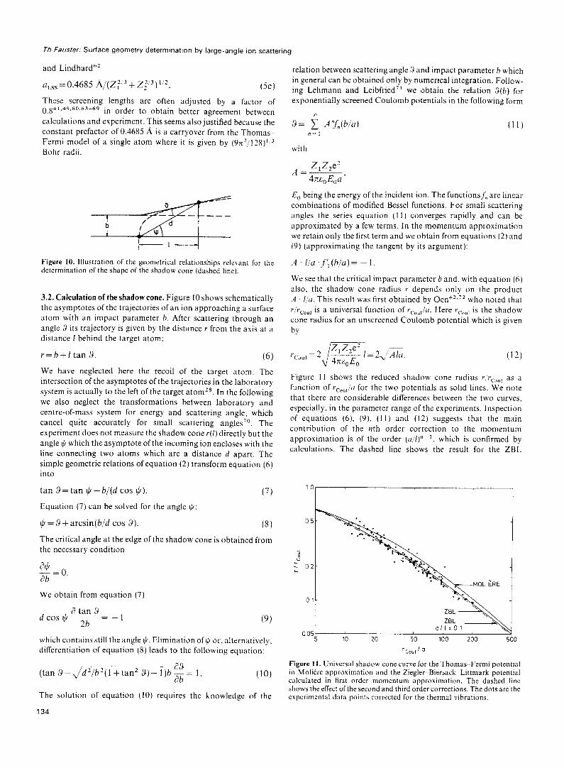
2.7. Sample orientation. In the preceding section we demonstrated the sample alignment by ICISS. This sensitivity to the sample orientation can be used to characterize miscut or stepped crystals. Figure 8 shows two angular scans obtained on a Cu( 1 IO) sample for two opposite directions. The crystal surface was carefully aligned by laser reflection and this alignment was verified by the minima in the sample current for a surface orientation parallel to the ion beam. Instead of two identical spectra the following differences are observed. The shadowing critical angles differ by 3”


5 keV Ne*- Cu (110)

, 11 1 ” “1 1 ““““I I

0 - 500 - 1000 - 1500

AZIMUTHAL ANGLE cp

Figure 7. The number ofelastically scattered Ne+ ions as a function of the azimuth angle cp for a fixed incidence angle $=8”. The low-index azimuthal orientations show up as well pronounced minima in the scattering yield due to the shadowing by the neighbour atoms.

. 5 keV Ne+e Cu (110) .

6.J. 9 : 16L’

l step up

ANGLE OF INCIDENCE W

Figure &The critical angles for shadowing measured relative to the sample surface differ up to 3” for equivalent azimuths on a crystal cut 1.5” off the normal orientation. The resulting defects show up as step-up and step- down atoms.

and in one direction we see intensity below the critical angle and in the opposite direction we see additional intensity after the focusing peak. These findings can be explained when we assume that the crystal planes are not parallel to the surface, i.e. the crystal is miscut or stepped. The misorientation causes steps to be seen at the surface. We observe additional intensity below Ic/, when we look up the steps (seeing the step edge atoms)57 and above $, when we look down the step (seeing the next-nearest neighbours of the step-edge atoms)33. In Figure 9 this behaviour is illustrated in more detail. We see the deviation of the critical angles AI/I from an adjusted mean value as a function of the azimuthal angle. It follows a sinusoidal dependence as expected since the surface normal precesses around the azimuthal rotation axis. The step-up signal (lower part of Figure 9) is observed only for a positive A+ when we look up the steps. The remaining step-up intensity for negative A$ results from some residual defects on the surface which might be due to crystal imperfections or are created during the measurements. From the known misalignment we can calibrate the step density absolutely which would be - 6% in our

T’ ’ ’ ’ ’ ’ ’ ’ ’ ’ ’ ‘I * +

--- -A- x

0 ;r Iii01 IO011 Ii101 looil

x + 0 0

0 l _.2-A-x-__~

Lb I I t I I II 11 (11 90" 0' -90" -moo

AZIMUTHAL ANGLE up

Figure 9.The variation of the critical angle with azimuthal orientation for a miscut crystal follows a sinusoidal dependence. The signal for small angles of incidence has its maximum for the direction looking up the steps.

case. It is also possible to determine the preferential direction along which steps develop5* and the compositional defect concentration on compound surfaces5’.

3. Scattering potentials

3.1. Screened Coulomb potentials. From the measurement of the critical angles (Figure 6) we can calculate the dimensions of the shadow cone via equation (2). A compilation of values for various distances and energies should allow in principle the determination of the scattering potential. The interaction between ions and atoms in the energy range above 100 eV is repulsive (see section 2.2) and is usually described by a screened Coulomb potential which has the correct asymptotic behaviour for small distances:

Z,Z2e2 W) = m X(m).

0

The parameter a is called the screening length. Support for this type of potential comes also from the Hartree-Fock calculations”. From the various screening functions proposed, we are selecting the Molibre approximation to theThomas-Fermi model (TFM)26.

xTFM(x)=0.35 exp(-0.3 x)+0.55 exp(- 1.2 x)

+O.l exp(-6.0 x) (4a)

and the empirical Ziegler-Biersack-Littmark (ZBL) function6’

xzaL(x)=0.0281 exp(-0.2016 x)

+ 0.2802 exp( - 0.4029 x)

+0.5099 exp(-0.9423 x)+0.1818 exp(-3.2 x).

(4b)

The last point to be considered is the choice of the screening length. For the ZBL potential the screening length should be chosen as

a zBL = 0.4685 A/(.Z:.23 + Z;.23). (5a)

For the Thomas-Fermi-Molitre potential commonly used screening lengths were proposed by Firsov”

UFirsov =0.4685 A/(z:‘Z + z;‘2)2’3 (5b)

133


and Lindhardb’ relation between scattering angle 3 and impact parameter h which in general can be obtained only by numerical integration. Follow- ing Lehmann and Leibfried” we obtain the relation 3(b) for exponentially screened Coulomb potentials in the following form

a Lss = 0.4685 a/(Z; 3 + Z;j3) ‘.“.

These screening lengths are often adjusted by a factor of 0.85’.“y.60.63-6y in order to obtain better agreement between calculations and experiment. This seems also justified because the constant prefactor of 0.4685 A is a carryover from the Thomas- Fermi model of a single atom where it is given by (9n’/l28)’ 3 Bohr radii.

Figure 10. Illustration of the geometrical relationships relevant for the determination of the shape of the shadow cone (dashed line).

3.2. Calculation of the shadow cone. Figure 10 shows schematically the asymptotes of the trajectories of an ion approaching a surface atom with an impact parameter h. After scattering through an angle 3 its trajectory is given by the distance r from the axis at a distance I behind the target atom:

r=b+l tan 3. (6)

We have neglected here the recoil of the target atom. The intersection of the asymptotes of the trajectories in the laboratory system is actually to the left of the target atom’*. In the following we also neglect the transformations between laboratory and centre-of-mass system for energy and scattering angle, which cancel quite accurately for small scattering angles’“. The experiment does not measure the shadow cone r(l) directly but the angle $ which the asymptote of the incoming ion encloses with the line connecting two atoms which are a distance ti apart. The simple geometric relations ofequation (2) transform equation (6) into

tan 3 = tan $ - b/(d cos $).

Equation (7) can be solved for the angle I/J:

i+k = 3 + arcsin(b/rf cos 3).

(7)

(8)

The critical angle at the edge of the shadow cone is obtained from the necessary condition

We obtain from equation (7)

(7 tan 3 d cos * ~ = -

2b 1 (9)

which contains still the angle ti. Elimination of $ or, alternatively. differentiation of equation (8) leads to the following equation:

(tan 3-Jd’/h’(l +tan2 9)-- l)h g= 1. (10)

The solution of equation (IO) requires the knowledge of the

134

with

E, being the energy of the incident ion. The functionsf, are linear combinations of modified Bessel functions. For small scattering angles the series equation (I 1) converges rapidly and can be approximated by a few terms. In the momentum approximation we retain only the first term and we obtain from equations (2) and (9) (approximating the tangent by its argument):

A l/a .f;(b/‘~~)= - 1.

We see that the critical impact parameter b and. with equation (6) also. the shadow cone radius r depends only on the product ,A //cr. This result was first obtained by 0en5’.” who noted that r/rcou, is a universal function of rcou,/u. Here rcou, is the shadow cone radius for an unscreened Coulomb potential which is given

by

rco”, = 2 ZlZ2e2 ___ 1=2,,iZ 47~~ E,

(12)

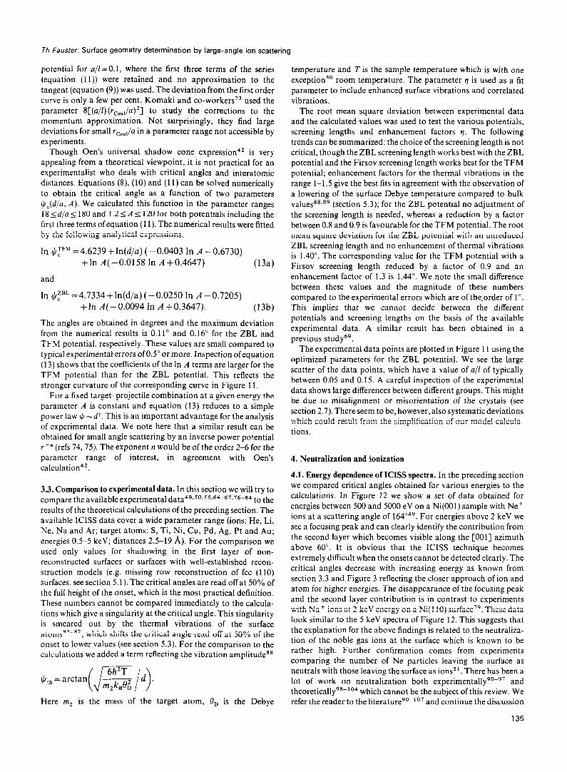
Figure 1 I shows the reduced shadow cone radius rjrcou, as a function of r cou,/o for the two potentials as solid lines. We note that there are considerable differences between the two curves. especially. in the parameter range of the experiments. Inspection of equations (6). (9) (II) and (12) suggests that the main contribution of the rrth order correction to the momentum approximation is of the order (n/l)“-‘, which is confirmed by calculations. The dashed line shows the result for the ZBL

a/l=01 005

5 10 20 50 100 200 500

‘CO”1 ’ a Figure 11. Universal shadow cone curve for the Thomas-Fermi potential in Moliere approximation and the Ziegler-Biersack-Littmark potential calculated in first order momentum approximation. The dashed line shows the effect of the second and third order corrections. The dots are the experimental data points corrected for the thermal vibrations.


potential for a/l =O.l, where the first three terms of the series

(equation (11)) were retained and no approximation to the tangent (equation (9)) was used. The deviation from the first order curve is only a few per cent. Komaki and co-workers73 used the parameter 8[(a/l)(rc,,,/a)2] to study the corrections to the momentum approximation. Not surprisingly, they find large deviations for small rcoU,/ a in a parameter range not accessible by experiments.

Though Oen’s universal shadow cone expression4’ is very appealing from a theoretical viewpoint, it is not practical for an experimentalist who deals with critical angles and interatomic distances. Equations (8), (10) and (11) can be solved numerically to obtain the critical angle as a function of two parameters $,(d/a, A). We calculated this function in the parameter ranges 18<d/a< 180 and 1.21A I 120 for both potentials including the first three terms of equation (11). The numerical results were fitted by the following analytical expressions.

In $‘“” = 4.6239 + ln(d/a) (- 0.0403 In A - 0.6730) c +In A(-0.0158 In A +0.4647) (I3a)

and

In I,/J~“” = 4.7334 + ln(d/a) ( - 0.0250 In A - 0.7205)

+ln A(-0.0094 In A +0.3647). (13b)

The angles are obtained in degrees and the maximum deviation from the numerical results is 0.11” and 0.16” for the ZBL and TFM potential, respectively. These values are small compared to typical experimental errors of0.5” or more. Inspection ofequation (13) shows that the coefficients of the In A terms are larger for the TFM potential than for the ZBL potential. This reflects the stronger curvature of the corresponding curve in Figure 11.

For a fixed target-projectile combination at a given energy the parameter A is constant and equation (13) reduces to a simple power law $ _ dY. This is an important advantage for the analysis of experimental data. We note here that a similar result can be obtained for small angle scattering by an inverse power potential r-” (refs 74,75). The exponent n would be of the order 2-6 for the parameter range of interest, in agreement with Oen’s calculation4*.

3.3. Comparison to experimental data. In this section we will try to compare the available experimental data49*50~55*64-67*76-84 to the results of the theoretical calculations of the preceding section. The available ICISS data cover a wide parameter range (ions: He, Li, Ne, Na and Ar; target atoms: S, Ti, Ni, Cu, Pd, Ag, Pt and Au; energies 0.5-5 keV; distances 2.5-19 A). For the comparison we used only values for shadowing in the first layer of non- reconstructed surfaces or surfaces with well-established reconstruction models (e.g. missing row reconstruction of fee (110) surfaces, see section 5.1). The critical angles are read off at 50% of the full height of the onset, which is the most practical definition. These numbers cannot be compared immediately to the calculations which give a singularity at the critical angle. This singularity is smeared out by the thermal vibrations of the surface atoms85-87, which shifts the critical angle read off at 50% of the onset to lower values (see section 5.3). For the comparison to the calculations we added a term reflecting the vibration amplitudes8

lClth = arctan( Jg id), Here m2 is the mass of the target atom, 0, is the Debye

temperature and T is the sample temperature which is with one exception5’ room temperature. The parameter I is used as a fit parameter to include enhanced surface vibrations and correlated vibrations.

The root mean square deviation between experimental data and the calculated values was used to test the various potentials, screening lengths and enhancement factors q. The following trends can be summarized: the choice of the screening length is not critical, though the ZBL screening length works best with the ZBL potential and the Firsov screening length works best for the TFM potential; enhancement factors for the thermal vibrations in the range l-l.5 give the best fits in agreement with the observation of a lowering of the surface Debye temperature compared to bulk values88~89 (section 5.3); for the ZBL potential no adjustment of the screening length is needed, whereas a reduction by a factor between 0.8 and 0.9 is favourable for the TFM potential. The root mean square deviation for the ZBL potential with an unreduced ZBL screening length and no enhancement of thermal vibrations is 1.40”. The corresponding value for the TFM potential with a Firsov screening length reduced by a factor of 0.9 and an enhancement factor of 1.3 is 1.44”. We note the small difference between these values and the magnitude of these numbers compared to the experimental errors which are of the,order of 1”. This implies that we cannot decide between the different potentials and screening lengths on the basis of the available experimental data. A similar result has been obtained in a previous study69.

The experimental data points are plotted in Figure 11 using the optimized parameters for the ZBL potential. We see the large scatter of the data points, which have a value of a/l of typically between 0.05 and 0.15. A careful inspection of the experimental data shows large differences between different groups. This might be due to misalignment or misorientation of the crystals (see section 2.7). There seem to be, however, also systematic deviations which could result from the simplification of our model calculations.

4. Neutralization and ionization

4.1. Energy dependence of ICISS spectra. In the preceding section we compared critical angles obtained for various energies to the calculations. In Figure 12 we show a set of data obtained for energies between 500 and 5000 eV on a Ni(OO1) sample with Ne+ ions at a scattering angle of 164”49. For energies above 2 keV we see a focusing peak and can clearly identify the contribution from the second layer which becomes visible along the [OOl] azimuth above 60”. It is obvious that the ICISS technique becomes extremely difficult when the onsets cannot be detected clearly. The critical angles decrease with increasing energy as known from section 3.3 and Figure 3 reflecting the closer approach of ion and atom for higher energies. The disappearance of the focusing peak and the second layer contribution is in contrast to experiments with Na’ ions at 2 keV energy on a Ni(ll0) surface”. These data look similar to the 5 keV spectra of Figure 12. This suggests that the explanation for the above findings is related to the neutralization of the noble gas ions at the surface which is known to be rather high. Further confirmation comes from experiments comparing the number of Ne particles leaving the surface as neutrals with those leaving the surface as ions5’. There has been a lot of work on neutralization both experimentally90-97 and theoretically98-104 which cannot be the subject of this review. We refer the reader to the literature90-L07 and continue the discussion

135

T/I Fauster- Surface geometry determination by large-angle ion scattering

00 300 60° 900

ANGLE OF INCIDENCE V

Figure 12. Number of elastically scattered Ne+ ions as a function of incidence angle $ for primary energies between 0.5 and 5 keV. Along the [IOO] azimuth of the Ni(OO1) surface the atoms in the second layer become visible for incidence angles over 60”.

in the following section with experimental evidence that the observation of the focusing peak above 3 keV energy is not only due to a decrease in the neutralization probability but to the onset of an ionization mechanism.

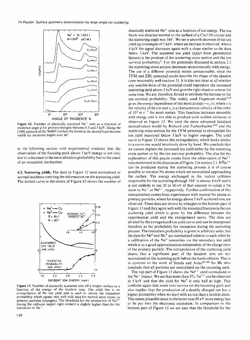
4.2. Scattering yields. The data in Figure 12 were normalized at normal incidence omitting the information on the scattering yield. The dotted curve in the centre of Figure 13 shows the number of

l Ne’ - cu -0 06

b Ne" .

-cu INlENSlTV Ne’. 9 = 16P INTENSITY Ne’

v = 900

-1 30

10 2.0 30 LO 50

INCIDENT ION ENERGY Ike'41

Figure 13. Number of elastically scattered ions off a copper surface as a function of the energy of the incident ions. The solid line is an extrapolation of the ion yield and is used to obtain the ionization probability which agrees very well with data for neutral neon atoms as primary particles (triangles). The threshold for the production of Ne’+ during the collision (upper right corner) is slightly higher than for the ionization to Ne+

136

elastically scattered Ne’ ions as a function of ion energy. The ion beam was directed normal to the surface of a Cu( 110) crystal and the scattering angle was 164”. We see a smooth decrease of the ion yield up to energies of 3 keV, where an increase is observed. Above 4 keV the signal decreases again with a slope similar to the data below 3 keV. The scattered ion yield (apart from geometrical factors) is the product of the scattering cross section and the ion survival probability’. For the potentials discussed in section 2.2 the scattering cross section decreases monotonically with energy. The use of a different potential seems unreasonable, since the TFM and ZBL potential could describe the shape of the shadow cone reasonably well (section 3). It is also not clear at all whether any sensible form of the potential could reproduce the increased scattering yield above 3 keV and give the right shadow cone at the same time. We are, therefore, forced to attribute the increase to the ion survival probability. The widely used Hagstrum model”‘” gives the energy dependence of this term as exp( - u,/u), where t’ is the velocity of the ion and L’, is a characteristic velocity of the order of 10’ m s- ’ for most metals. This function increases smoothly with energy and is not able to produce such sudden increases as observed in Figure 13. We used the more advanced localized neutralization model by Richard and Eschenbacher”’ and the scattering cross section for the TFM potential to extrapolate the ion yield measured below 3 keV to higher energies. The solid curve in Figure 13 shows this extrapolation, which looks similar to a curve one would intuitively draw by hand. We conclude that we cannot explain the increased ion yield either by the scattering cross section or by the ion survival probability. The clue for the explanation of this puzzle comes from the observation of Ne” ions mentioned in the discussion of Figure 2 in section 2.1. If Ne’ + can be produced during the scattering process it is of course possible to reionize Ne atoms which are neutralized approaching the surface. The energy exchanged in the violent collision responsible for the scattering through 164” is almost 4 keV and it is not unlikely to use 20 or 60 eV of that amount to ionize a Ne atom to Ne+ or Ne2 +, respectively. Further confirmation of this interpretation comes from experiments with neutral Ne atoms as primary particles, where for energy above 3 keV scattered ions are observed. These data are shown by triangles in the bottom part of Figure 13 and they agree well with the reionized fraction in the ion scattering yield which is given by the difference between the experimental yield and the extrapolated curve. The data are divided by the extrapolated ion yield curve and can be interpreted therefore as the probability for ionization during the scattering process. The ionization probability is given in arbitrary units. but the data for Ne” and Ne+ are normalized relative to each other by a calibration of the Ne” intensities via the secondary ion yield which is to a good approximation independent of the charge state of the primary particle. The extrapolation of the scattering yield shows that a significant part of the incident ions are not neutralized on the incoming path before the hard collision. This is in contrast to the work of Souda and Aono43.44 for He who conclude that all particles are neutralized on the incoming path.

The top part of Figure 13 shows the Ne2+ yield normalized to the Ne+ impact. We see that more than 5% Ne2 + can be observed at 5 keV and that the yield for Ne” is only half as high. This confirms again that some ions survive on the incoming path and also implies that the production of a doubly charged ion has a higher probability when we start with an ion than a neutral atom. This seems plausible since in the latter case 20 eV more energy has to be put into the electronic excitation. In comparison to the bottom part of Figure 13 we see also that the threshold for the


production of Ne’+ is - 500 eV higher than for the reionization to Ne+ as measured by the increase of the ion yield, which agrees with the higher ionization energy for Ne’+.

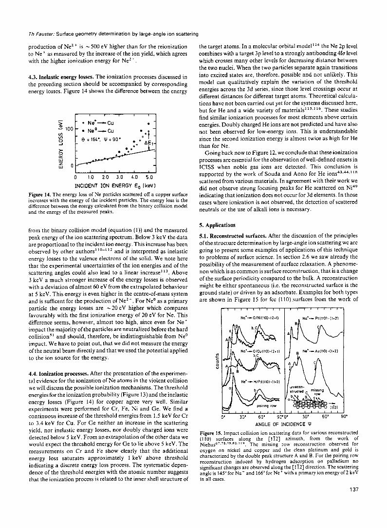
4.3. Inelastic energy losses. The ionization processes discussed in the preceding section should be accompanied by corresponding energy losses. Figure 14 shows the difference between the energy

F 2 100

+ Ne*-Cu

z

l Ne” --cu

0 = 164’. UJ = 90’ l ++i

. l .r J

1 I 1 I I I

0 1.0 2.0 3.0 L.0 5.0

INCIDENT ION ENERGY E, tkeV I

Figure 14. The energy loss of Ne particles scattered off a copper surface increases with the energy of the incident particles. The energy loss is the difference between the energy calculated from the binary collision model and the energy of the measured peaks.

from the binary collision model (equation (1)) and the measured peak energy of the ion scattering spectrum. Below 3 keV the data are proportional to the incident ion energy. This increase has been observed by other authors1’0-“2 and is interpreted as inelastic energy losses to the valence electrons of the solid. We note here that the experimental uncertainties of the ion energies and of the scattering angles could also lead to a linear increase’13. Above 3 keV a much stronger increase of the energy losses is observed with a deviation of almost 60 eV from the extrapolated behaviour at 5 keV. This energy is even higher in the centre-of-mass system and is sufficent for the production of Ne’+. For Ne” as a primary

particle the energy losses are - 20 eV higher which compares favourably with the first ionization energy of 20 eV for Ne. This difference seems, however, almost too high, since even for Ne+ impact the majority of the particles are neutralized before the hard collision5 l and should, therefore, be indistinguishable from Ne” impact. We have to point out, that we did not measure the energy of the neutral beam directly and that we used the potential applied to the ion source for the energy.

4.4. Ionization processes. After the presentation of the experimental evidence for the ionization of Ne atoms in the violent collision we will discuss the possible ionization mechanisms. The threshold energies for the ionization probability (Figure 13) and the inelastic energy losses (Figure 14) for copper agree very well. Similar experiments were performed for Cr, Fe, Ni and Ge. We find a continuous increase of the threshold energies from 1.5 keV for Cr to 3.4 keV for Cu. For Ge neither an increase in the scattering yield, nor inelastic energy losses, nor doubly charged ions were detected below 5 keV. From an extrapolation of the other data we would expect the threshold energy for Ge to lie above 5 keV. The measurements on Cr and Fe show clearly that the additional energy loss saturates approximately 1 keV above threshold indicating a discrete energy loss process. The systematic dependence of the threshold energies with the atomic number suggests that the ionization process is related to the inner shell structure of

the target atoms. In a molecular orbital model’ l4 the Ne 2p level combines with a target 3p level to a strongly antibonding 4fa level which crosses many other levels for decreasing distance between the two nuclei. When the two particles separate again transitions into excited states are, therefore, possible and not unlikely. This model can qualitatively explain the variation of the threshold energies across the 3d series, since those level crossings occur at different distances for different target atoms. Theoretical calculations have not been carried out yet for the systems discussed here, but for He and a wide variety of materials’i5*’ 16. These studies find similar ionization processes for most elements above certain energies. Doubly charged He ions are not predicted and have also not been observed for low-energy ions. This is understandable since the second ionization energy is almost twice as high for He than for Ne.

Going back now to Figure 12, we conclude that these ionization processes are essential for the observation ofwell-defined onsets in ICISS when noble gas ions are detected. This conclusion is supported by the work of Souda and Aono for He ions43,44.1’s scattered from various materials. In agreement with their work we did not observe strong focusing peaks for He scattered on Ni49 indicating that ionization does not occur for 3d elements. In those cases where ionization is not observed, the detection of scattered neutrals or the use of alkali ions is necessary.

5. Applications

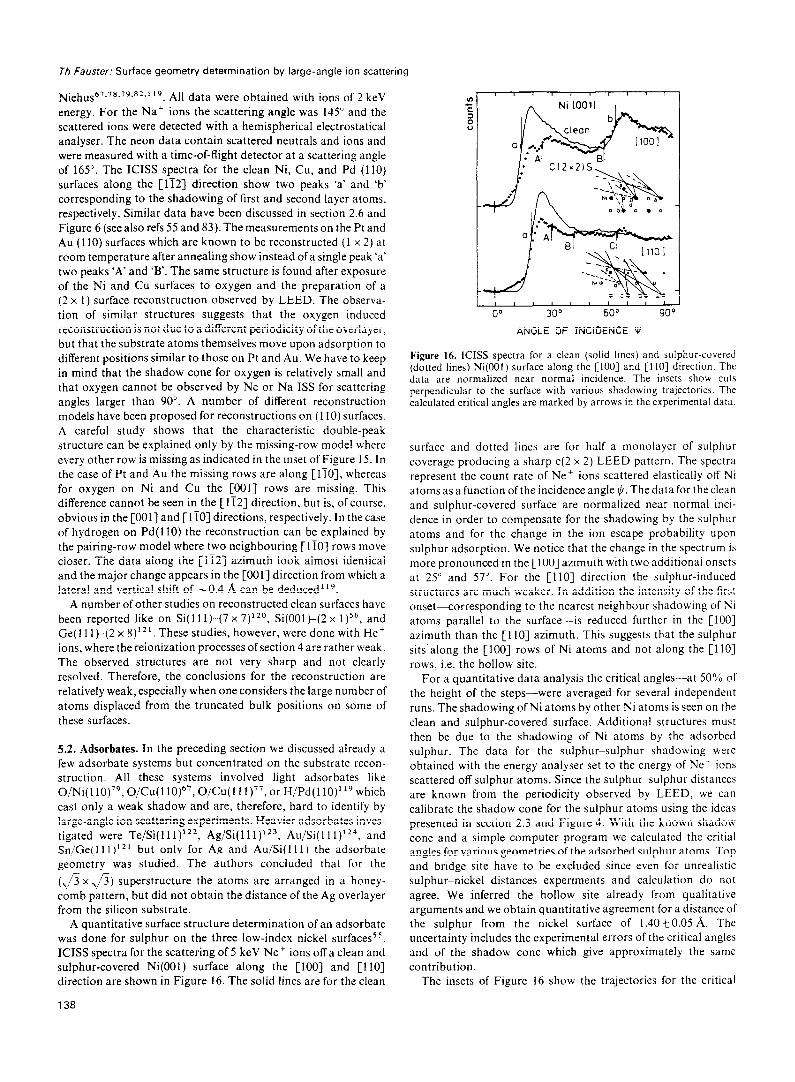
5.1. Reconstructed surfaces. After the discussion of the principles of the structure determination by large-angle ion scattering we are going to present some examples of applications of this technique to problems of surface science. In section 2.6 we saw already the possibility of the measurement of surface relaxation. A phenome- non which is as common is surface reconstruction, that is a change of the surface periodicity compared to the bulk. A reconstruction might be either spontaneous (i.e. the reconstructed surface is the ground state) or driven by an adsorbate. Examples for both types are shown in Figure 15 for fee (1lO)surfaces from the work of

No’--O/NilllOl-12.1)

Nc’-H/PdIlIOI-Il.21

I e Ni-Aui110141.21

30’ 60’ 90’0’ 30’ 60’ !

ANGLE OF INCIOENCE ‘4’

Figure 15. Impact collision ion scattering data for various reconstructed (110) surfaces along the [Ii21 azimuth, from the work of Niehus67.78~79~82~“9. The missing row reconstruction observed for oxygen on nickel and copper and the clean platinum and gold is characterized by the double peak structure A and B. For the pairing row reconstruction induced by hydrogen adsorption on palladium no significant changes are observed along the [lT2] direction. The scattering angle is 145” for Na+ and 166” for Ne+ with a primary ion energy of 2 keV in all cases.

137


Niehus67*78*7g~82~“g. All data were obtained with ions of 2 keV energy. For the Na+ ions the scattering angle was 145” and the scattered ions were detected with a hemispherical electrostatical analyser. The neon data contain scattered neutrals and ions and were measured with a time-of-flight detector at a scattering angle of 165”. The ICISS spectra for the clean Ni, Cu, and Pd (110) surfaces along the [li2] direction show two peaks ‘a’ and ‘b corresponding to the shadowing of first and second layer atoms, respectively. Similar data have been discussed in section 2.6 and Figure 6 (see also refs 5.5 and 83). The measurements on the Pt and Au (110) surfaces which are known to be reconstructed (1 x 2) at room temperature after annealing show instead of a single peak ‘a’ two peaks ‘A’ and ‘B’. The same structure is found after exposure of the Ni and Cu surfaces to oxygen and the preparation of a (2 x 1) surface reconstruction observed by LEED. The observation of similar structures suggests that the oxygen induced reconstruction is not due to a different periodicity of the overlayer, but that the substrate atoms themselves move upon adsorption to different positions similar to those on Pt and Au. We have to keep in mind that the shadow cone for oxygen is relatively small and that oxygen cannot be observed by Ne or Na ISS for scattering angles larger than 90”. A number of different reconstruction models have been proposed for reconstructions on (110) surfaces. A careful study shows that the characteristic double-peak structure can be explained only by the missing-row model where every other row is missing as indicated in the inset of Figure 15. In the case of Pt and Au the missing rows are along [ liO], whereas for oxygen on Ni and Cu the [OOl] rows are missing. This difference cannot be seen in the [li2] direction, but is, of course. obvious in the [OOl] and [ liO] directions, respectively. In the case of hydrogen on Pd( 110) the reconstruction can be explained by the pairing-row model where two neighbouring [ liO] rows move closer. The data along the [li2] azimuth look almost identical and the major change appears in the [OOl] direction from which a lateral and vertical shift of -0.4 8, can be deduced”‘.

A number of other studies on reconstructed clean surfaces have been reported like on Si( 111 k(7 x 7)12’, Si(OO1 t(2 x 1)56, and Ge( ill)-(2 x 8)‘*‘. These studies, however, were done with He+ ions, where the reionization processes of section 4 are rather weak. The observed structures are not very sharp and not clearly resolved. Therefore, the conclusions for the reconstruction are relatively weak, especially when one considers the large number of atoms displaced from the truncated bulk positions on some of

these surfaces.

5.2. Adsorbates. In the preceding section we discussed already a few adsorbate systems but concentrated on the substrate reconstruction. All these systems involved light adsorbates like 0/‘Ni(110)7g, O/C~(110)~‘, O/Cu(l ll)“, or H/Pd(l10)‘19 which cast only a weak shadow and are, therefore, hard to identify by large-angle ion scattering experiments. Heavier adsorbates inves- tigated were Te/Si( 11 l)‘**, Ag/Si( 11 I)‘*‘, Au,/Si( 11 1)‘24, and Sn/Ge( 111) I*] but only for Ag and Au/Si(lll) the adsorbate geometry was studied. The authors concluded that for the

(+5x J?) superstructure the atoms are arranged in a honey- comb pattern, but did not obtain the distance of the Ag overlayer from the silicon substrate.

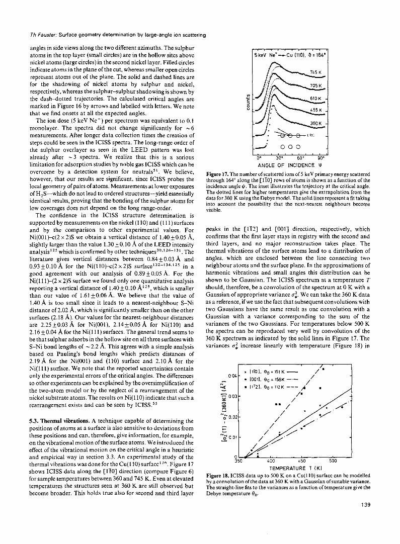
A quantitative surface structure determination of an adsorbate was done for sulphur on the three low-index nickel surfaces”. ICISS spectra for the scattering of 5 keV Ne+ ions off a clean and sulphur-covered Ni(OO1) surface along the [IOO] and [l lo] direction are shown in Figure 16. The solid lines are for the clean

138

00 300 60° 900

ANGLE OF INCIDENCE W

Figure 16. ICISS spectra for a clean (solid lines) and sulphur-covered (dotted lines) Ni(OO1) surface along the [loo] and [IlO] direction. The data are normalized near normal incidence. The insets shobv cuts perpendicular to the surface with various shadowing trajectories. The calculated critical angles are marked by arrows in the experimental data.

surface and dotted lines are for half a monolayer of sulphur coverage producing a sharp c(2 x 2) LEED pattern. The spectra represent the count rate of Ne+ ions scattered elastically off Ni atoms as a function of the incidence angle II/. The data for the clean and sulphur-covered surface are normalized near normal incidence in order to compensate for the shadowing by the sulphur atoms and for the change in the ion escape probability upon sulphur adsorption. We notice that the change in the spectrum is more pronounced in the [IOO] azimuth with two additional onsets at 25” and 57”. For the [I lo] direction the sulphur-induced structures are much weaker. In addition the intensity of the first onset--corresponding to the nearest neighbour shadowing of Ni atoms parallel to the surface-is reduced further in the [loo] azimuth than the [l lo] azimuth. This suggests that the sulphur sits along the [loo] rows of Ni atoms and not along the [l 10) rows, i.e. the hollow site.

For a quantitative data analysis the critical angles-at 50% of the height of the steps-were averaged for several independent runs. The shadowing of Ni atoms by other Ni atoms is seen on the clean and sulphur-covered surface. Additional structures must then be due to the shadowing of Ni atoms by the adsorbed sulphur. The data for the sulphur-sulphur shadowing were obtained with the energy analyser set to the energy of Ne+ ions scattered off sulphur atoms. Since the sulphur-sulphur distances are known from the periodicity observed by LEED, we can calibrate the shadow cone for the sulphur atoms using the ideas presented in section 2.3 and Figure 4. With the known shadow cone and a simple computer program we calculated the critial angles for various geometries of the adsorbed sulphur atoms. Top and bridge site have to be excluded since even for unrealistic sulphur-nickel distances experiments and calculation do not agree. We inferred the hollow site already from qualitative arguments and we obtain quantitative agreement for a distance of the sulphur from the nickel surface of 1.40~0.05 A. The uncertainty includes the experimental errors of the critical angles and of the shadow cone which give approximately the same contribution.

The insets of Figure 16 show the trajectories for the critical


angles in side views along the two different azimuths. The sulphur atoms in the top layer (small circles) are in the hollow sites above nickel atoms (large circles) in the second nickel layer. Filled circles indicate atoms in the plane of the cut, whereas smaller open circles represent atoms out of the plane. The solid and dashed lines are for the shadowing of nickel atoms by sulphur and nickel, respectively, whereas the sulphur-sulphur shadowing is shown by the dash-dotted trajectories. The calculated critical angles are marked in Figure 16 by arrows and labelled with letters. We note that we find onsets at all the expected angles.

The ion dose (5 keV Ne+) per spectrum was equivalent to 0.1 monolayer. The spectra did not change significantly for -6 measurements. After longer data collection times the creation of steps could be seen in the ICISS spectra. The long-range order of the sulphur overlayer as seen in the LEED pattern was lost already after -3 spectra. We realize that this is a serious limitation for adsorption studies by noble gas ICISS which can be overcome by a detection system for neutrals’i. We believe, however, that our results are significant, since ICISS probes the local geometry of pairs of atoms. Measurements at lower exposures of H,S-which do not lead to ordered structures-yield essentially identical results, proving that the bonding of the sulphur atoms for low coverages does not depend on the long range-order.

The confidence in the ICISS structure determination is supported by measurements on the nickel (110) and (111) surfaces and by the comparison to other experimental values. For Ni(OOl)-c(2 x 2)s we obtain a vertical distance of 1.40&0.05 A, slightly larger than the value 1.30 +O.lO A of the LEED intensity analysis”’ which is confirmed by other techniques30~126-1 3 l. The literature gives vertical distances between 0.84+0.03 A and 0.93iO.10 A for the Ni(llO)-c(Z x 2)s surface132-134.125 in a good agreement with our analysis of 0.89f0.05 A. For the Ni( 11 lt(2 x 2)s surface we found only one quantitative analysis reporting a vertical distance of 1.40+0.10 A’*‘, which is smaller than our value of 1.61+0.06 A. We believe that the value of 1.40 A is too small since it leads to a nearest-neighbour S-Ni distance of 2.02 A, which is significantly smaller than on the other surfaces (2.18 A). Our values for the nearest-neighbour distances are 2.25+0.03A for Ni(OOl), 2.14+_0.05A for Ni(ll0) and 2.16 kO.04 A for the Ni(ll1) surfaces. The general trend seems to be that sulphur adsorbs in the hollow site on all three surfaces with S-Ni bond lengths of - 2.2 A. This agrees with a simple analysis based on Pauling’s bond lengths which predicts distances of 2.19A for the Ni(OO1) and (110) surface and 2.1OA for the Ni( 111) surface. We note that the reported uncertainties contain only the experimental errors of the critical angles. The differences to other experiments can be explained by the oversimplification of the two-atom model or by the neglect of a rearrangement of the nickel substrate atoms. The results on Ni( 110) indicate that such a rearrangement exists and can be seen by ICISS.55

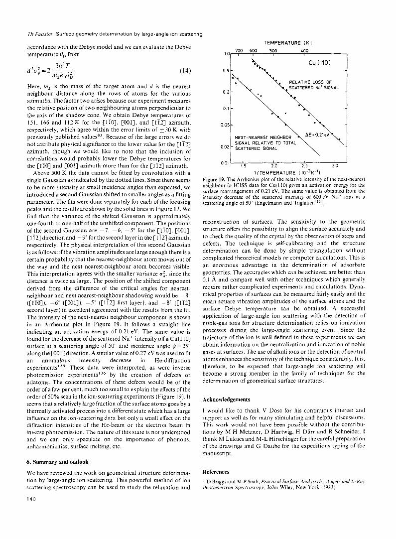
5.3. Thermal vibrations. A technique capable of determining the positions of atoms at a surface is also sensitive to deviations from these positions and can, therefore, give information, for example, on the vibrational motion of the surface atoms. We introduced the effect of the vibrational motion on the critical angle in a heuristic and empirical way in section 3.3. An experimental study of the thermal vibrations was done for the Cu(ll0) surface’36. Figure 17 shows ICISS data along the [liO] direction (compare Figure 6) for sample temperatures between 360 and 745 K. Even at elevated temperatures the structures seen at 360 K are still observed but become broader. This holds true also for second and third layer

5keV Ne* --cu (110). 19 = 164’

.

2 000

L 00 300 60° 90°

ANGLE OF INCIDENCE U’

Figure 17. The number ofscattered ions of 5 keV primary energy scattered through 164” along the [ 1iOJ rows of atoms is shown as a function of the incidence angle IJ. The inset illustrates the trajectory at the critical angle. The dotted lines for higher temperatures give the extrapolation from the data for 360 K using the Debye model. The solid lines represent a fit taking into account the possibility that the next-nearest neighbours become visible.

peaks in the [li2] and [OOl] direction, respectively, which confirms that the first layer stays in registry with the second and third layers, and no major reconstruction takes place. The thermal vibrations of the surface atoms lead to a distribution of angles, which are enclosed between the line connecting two neighbour atoms and the surface plane. In the approximations of harmonic vibrations and small angles this distribution can be shown to be Gaussian. The ICISS spectrum at a temperature T should, therefore, be a convolution of the spectrum at 0 K with a Gaussian of appropriate variance ~3. We can take the 360 K data as a reference, if we use the fact that subsequent convolutions with two Gaussians have the same result as one convolution with a Gaussian with a variance corresponding to the sum of the variances of the two Gaussians. For temperatures below 500 K the spectra can be reproduced very well by convolution of the 360 K spectrum as indicated by the solid lines in Figure 17. The variances CJ$ increase linearly with temperature (Figure 18) in

x IlTO]. BD=151K - / ‘.

OOL- l [OOll. 80 -166K -.-

% . [iizl. ec= 112K --- /i /'

.

FO03-

% 3 NN 0 002- ,

F:

NN sOO'-

O- 350 LOO LSO 500

TEMPERATURE T (K)

Figure 18. ICISS data up to 500 K on a Cu( 110) surface can be modelled by a convolution of the data at 360 K with a Gaussian ofsuitable variance. The straight-line fits to the variances as a function of temperature give the Debye temperature 0,.

139

Th Fauster: Surface geometry determination by large-angle ion scattertng

accordance with the Debye model and we can evaluate the Debye temperature 0, from

3h2T (pa;=2 ___

m,k,Oi, (14)

Here, m2 is the mass of the target atom and rl is the nearest neighbour distance along the rows of atoms for the various azimuths. The factor two arises because our experiment measures the relative position of two neighbouring atoms perpendicular to the axis of the shadow cone. We obtain Debye temperatures of 151, 166 and 112K for the [liO], [OOl], and [li2] azimuth, respectively, which agree within the error limits of i_ 30 K with previously published values *3 Because of the large errors we do not attribute physical signifiance to the lower value for the [li2] azimuth, though we would like to note that the inclusion of correlations would probably lower the Debye temperatures for the [ liO] and [OOl] azimuth more than for the [Ii21 azimuth.

Above 500 K the data cannot be fitted by convolution with a single Gaussian as indicated by the dotted lines. Since there seems to be more intensity at small incidence angles than expected, we introduced a second Gaussian shifted to smaller angles as a fitting parameter. The fits were done separately for each of the focusing peaks and the results are shown by the solid lines in Figure 17. We find that the variance of the shifted Gaussian is approximately one-fourth to one-half of the unshifted component. The positions of the second Gaussian are -7, -6, -5” for the [IiO], [OOI], [li2] direction and -9” for the second layer in the [Ii21 azimuth, respectively. The physical interpretation of this second Gaussian is as follows: if the vibration amplitudes are large enough there is a certain probability that the nearest-neighbour atom moves out of the way and the next nearest-neighbour atom becomes visible. This interpretation agrees with the smaller variance cri, since the distance is twice as large. The position of the shifted component derived from the difference of the critical angles for nearest- neighbour and next nearest-neighbour shadowing would be --8’ ([lie]), -6” ([OOl]), -5’ ([li2] first layer), and -8” ([li2] second layer) in excellent agreement with the results from the fit. The intensity of the next-nearest neighbour component is shown in an Arrhenius plot in Figure 19. It follows a straight line indicating an activation energy of 0.21 eV. The same value is found for the decrease of the scattered Na’ intensity off a Cu( 110) surface at a scattering angle of 50” and incidence angle $=25O along the [OOl] direction. A similar value of0.27 eV was used to fit an anomalous intensity decrease in He-diffraction experiments I36 These data were interpreted, as were inverse photoemission experiments I36 by the creation of defects or adatoms. The concentrations of these defects would be of the order of a few per cent, much too small to explain the effects of the order of 50% seen in the ion-scattering experiments (Figure 19). It seems that a relatively large fraction of the surface atoms goes by a thermally activated process into a different state which has a large influence on the ion-scattering data but only a small effect on the diffraction intensities of the He-beam or the electron beam in inverse photoemission. The nature of this state is not understood and we can only speculate on the importance of phonons. anharmonicities, surface melting. etc.

6. Summary and outlook

We have reviewed the work on geometrical structure determination by large-angle ion scattering. This powerful method of ion scattering spectroscopy can be used to study the relaxation and

140

TEMPERATURE C K I

cu (110)

RELATIVE LOSS OF

0.05 -

SIGNAL RELATIVE TO TOTAL 0.02 - SCATTERED SIGNAL

I I 0°’ 15 1 1 I

2.0 25 30

1 /TEMPERATURE I 10‘3K-‘) Figure 19. The Arrhenius plot of the relative intensity of the next-nearest neighbour in ICISS data for Cu(l10) gives an activation energy for the surface rearrangement of 0.21 eV. The same value is obtained from the intensity decrease of the scattered intensity of 600 eV Na’ ions at a scattering angle of 50” (Engelmann and Taglauer’36).

reconstruction of surfaces. The sensitivity to the geometric structure offers the possibility to align the surface accurately and to check the quality of the crystal by the observation of steps and defects. The technique is self-calibrating and the structure determination can be done by simple triangulation without complicated theoretical models or computer calculations. This is an enormous advantage in the determination of adsorbate geometries. The accuracies which can be achieved are better than 0.1 A and compare well with other techniques which generally require rather complicated experiments and calculations. Dyna- mical properties of surfaces can be measured fairly easily and the mean square vibration amplitudes of the surface atoms and the surface Debye temperature can be obtained. A successful application of large-angle ion scattering with the detection of noble-gas ions for structure determination relies on ionization processes during the large-angle scattering event. Since the trajectory of the ion is well defined in these experiments we can obtain information on the neutralization and ionization of noble gases at surfaces. The use of alkali ions or the detection of neutral atoms enhances the sensitivity of the technique considerably. It is, therefore, to be expected that large-angle ion scattering will become a strong member in the family of techniques for the determination of geometrical surface structures.

Acknowledgements

I would like to thank V Dose for his continuous interest and support as well as for many stimulating and helpful discussions. This work would not have been possible without the contributions by M H Metzner, D Hartwig, H Diirr and R Schneider. I thank M Lukacs and M-L Hirschinger for the careful preparation of the drawings and G Daube for the expeditious typing of the manuscript.

References

’ D Briggs and M P Seah, Pracfical Strr~fnce Andysis by Augrr- and X-k, Pltotorkctron .Specrroscopy, John Wiley, New York (1983).


z G Ertl and J Kiippers, Low Energy Electrons and Surface Chemisrry, VCH. Weinheim (1985). 3 A Benninghoven and others, Secondary Ion Mass Spectrometry SIMS If-V, Springer, Berlin (1979-1986). ’ D A King: Surf Sci, 47, 384 (1975). 5 E Taelauer. ADD! Phvs. A38. 161 (1985). . . _ . 6 W K Chen, J W Mayer and M-A Nicolet, Backscattering Specrrometry, Academic Press, New York (1978). ’ R Feidenhans’l, J. S. Pedersen, M Nielsen, F Grey and R L Johnson, Surf Sci, 178,927 (1986). * J B Pendry, Low Energy Electron Dlflaction, Academic Press, New York (1974). 9 M A Van Hove and S Y Tong, Surface Crystallography hy LEED, Springer, Berlin (1979). I0 G Comsa and B Poelsema, Appl Phys, A38, 153 (1985). I’ D J Smith, Chemistry and Physics of Solid Surfaces VI (Edited by R Vanselow and R Howe), p 413, Springer, Berlin (1986). ” P K Hansma and J Tersoff, Jappl Phys, 61, Rl (1987). I3 J F van der Veen, Surf Sci Rep, 5, 199 (1985). I4 J P Toennies, J Vat Sci Technol, AZ, 1055 (1984). l5 M Rocca. H Ibach, S Lehwald and T S Rahman, Srructure and Dynamics of Surfaces I (Edited by W Schommers and P von Blancken- hagen), p 245, Springer, Berlin (1986). I6 F J Himpsel, Adu Phys, 32, 1 (1983). ” V Dose. SurfSci Rep, 5. 337 (1985). I8 Th Fauster “and V hose, Chektr; and Physics of Solid Surfaces VI (Edited by R Vanselow and R Howej, p 483, Spring&, Berlin (i986). I9 D P Woodruff and T A Delchar, Modern Techniaues ofSurface Science. Cambridge University Press, Cambridge (1986). ’ ’ ’ --’ 2o D P Smith, SurfSci, 25, 171 (1971). 21 H H Brongersma and P M Mul, Surf Sci, 35, 393 (1973). ** E Taglauer and W Heiland, Appl Phys, 9,261 (1976). z3 D J O’Connor, Surf Sci, 173, 593 (1986). l4 W L Baun, Surf Sci, 72, 536 (1978). 25 B Poelsema, L K Verhey and A L Boers, Surf Sci, 64, 537 (1977). ” G Molikre, Z Nalurforsch, Za, 133 (1947). ” 0 B Firsov, Zh Experim Tear Fyz, 33,696 (195 1); Sol: Phys JETP, 6, 534 (1958). ‘* M T Robinson. Phys Reo, B9. 5008 (1974). 29 H H Brongersma and J B Theeten, Surf Sci, 54, 519 (1975). 3o J B Theeten and H H Brongersma, Ret Phys Appl, 11, 57 (1976). 31 W Englert, W Heiland, E Taglauer and D Menzel, Surf Sri, 83, 243 (1979). ‘* L K Verheij, J A van den Berg and D G Armour, Surf Sci, 84, 408 (1979). 33 A J Algra, S B Luitjens, E P Th M Suurmeijer and A L Boers. Surf Sci, 100, 329 (1980). 34 D J Godfrey and D P Woodruff, Surf Sci, 105,459 (1981). 35 S H Overbury, W Heiland, D M Zehner, S Datz and R S Thee. Surf Sci, 109, 239 (1981). 36 R P Bronckers and A G J de Wit, Surf Sci, 112, 133 (1981). 37 H Niehus and E Preuss, Surf Sci, 119, 349 (1982). 38 R S Williams and J A Yarmoff, Nucl Instrum Meth, 218, 235 (1983). 39 L Marchut TM Buck, G H Wheatley and C J McMahon Jr, Surf Sci, 141, 549 (1984). 4o M Aono, C Oshima, S Zaima, S Otani and Y Ishizawa, Japan J Appl Phys, 20, L829 (1981). 41 Y Yamamura and W Takeuchi, Radiar Effects 82, 73 (1984). 42 0 S Oen, Surf&i, 131, L407 (1983). 43 R Souda M Aono, C Oshima, S Otani and Y Ishizawa, Surf Sci, 150, L59 (1985).’ 44 R Souda and M Aono, Nucl Instrum Meth, B15, 114 (1986). 45 E Taglauer, W Melchior, F Schuster and W Heiland, J Phys, E8, 768 (1975). 46 H Niehus and E Bauer, Surf Sci, 47,222 (1975). &’ F Shoji and T Hanawa, Surf Sci, 129, L261 (1983). 48 J A YarmofI and R S Williams, Rev Sci Instrum, 57,433 (1986). 49 Th Fauster and M H Metzner, Surf Sci, 166, 29 (1986). 5o H Niehus and G Comsa, Nucl Instrum Merh, B15, 122 (1986). 5’ ‘rl Niehus. Surf&i. 166. L107 (1.986). 52 T M Buck, GH Wheatley and L K Verheij, SurfSci. 90, 635 (1979). 53 H L Davis and J R Noonan, Surf&i, 126, 245 (1983). 54 D L Adams, H B Nielsen and J G Andcrsen, SuriSci, i28,294 (1983). 55 Th Fauster, H Diirr and D Hartwig, SurfSci, 178, 657 (1986). 56 M Aono, Y Hou, C Oshima and Y Ishizawa, Phys Rev Lett, 49, 567 (1982).

57 Th M Hupkens and J M van Zoest, Nucl lnstrum Met/t, B6,538 (1985). 58 H Niehus and G Comsa. Nucl lnstrum Meth. B13, 213 (1986). 59 M Aono Y Hou, R Souda, C Oshima. S Otani and Y Ishizawa, Phy,~ Ret) Left, 56, 1293 (1983). 6o S A Cruz E V Alonso. R P Walker, D J Martin and D G Armour, Nucl lnstrum Me;h, 194, 659 (1982). ” J F Ziegler. J P Biersack and U Littmark. ORNL Report No, CONF-820131 (unpublished), J P Biersack and J F Ziegler, Springer Series in Nectrophysics, vol 10, p 122, Springer, Berlin (1982). 6L J Lindhard, M Scharff and H E Schiott. Ka/Danske Videnskab Selbskab Mat Fys Medd, 33, (1965). ” D P Jackson, W Heiland and E Taglauer, Phrs Ret) B24,4198 (1981). 6J R P N Bronckers and A G J de Wit, Surf.%;, 104, 384 (1981). ” M Aono Y Hou, R Souda, C Oshima, S dtani, Y Ishizawa, K Matsuda and R Shi&zu, Japan J Appl Phys, 21, L670 (1982). 66 M Aono, Nucl Instrum Merh, B2, 374 (1984). ” H Niehus and G Comsa, Surf Sci, 140, I8 (1984). ‘s S H Overbury, Nucl Jnstrum Merh, B2, 448 (1984). 6y S H Overbury and D R Huntley, Phys Rev, B32, 6278 (1985). ‘O H J Gossmann, Thesis, University of New York at Albany (unpublished) (1985). ” C Lehmann and G Leibfried. Z Phys, 172,465 (1963). ‘* 0 S Oen, Proc. 7th Int Conf on Atomic Collisions in Solids, vol 2. (Edited by Y V Bulgakov and A F Tulinov) p 124. Moscow State University Publishing House, Moscow (1981). ” K Komaki, A Ootuka and F Fujimoto, Japan J Appl Phys, 21, L52l (1982). ” Y V Martynenko, Radiar Eflects, 20, 21 I (1973). I

” E S Mashkova and V A Molchanov, Radial E’ects, 23, 215 (1974). 76 M Aono, R Souda, C Oshima and Y Ishizawa, Surf Sci, 168,7 I3 (1986). ” H Niehus, Surf Sci, 130, 41 (1983). ‘s H Niehus. Surf Sci, 145. 407 (1984). ‘9 H Niehus and G Comsa, Surf Sci, 151, L17l (1985). *’ H Niehus and G Comsa, Surf Sci, 152, 93 (1985). ” J Miiller. H Niehus and W Heiland, Surf Sci, 166, Ll I1 (1986). ” J Miiller, K J Snowdon, W Heiland and H Niehus, Surf Sci, 178,475 (1986). *’ J A Yarmoff. D M Cyr, J H Huang. S Kim and R S Williams, Phys Rer: 833, 3856 (1986). *‘Th Fauster. D Hartwig and H Diirr, unpublished data. 85 W Takeuchi and Y Yamamura, Nucl fnsfrunr Met/l, B2, 336 (1984). *6 W Takeuchi and Y Yamamura, Surf Sci, 169. 365 (1986). *’ R Souda. M Aono. C Oshima. S Otani and Y Ishizawa, Surf Sci, 128, L236 (1983). ** G Engelmann, E Taglauer and D P Jackson, Surf Sci, 162,921 (1985). 89 B Poelsema. L K Verhev and A L Boers. Nucl Instrum Meth, 132, 623 (1976). ” C-C Chang, L A DeLouise, N Winograd and B J Garrison, Surf Sci, 154, 22 (1985). ” J W Rabalais. J-N Chen, R Kumar and M Narayana, J Chem Phys, 83, 6489 (1985). ‘* S H Overbury, B M Dekoven and P C Stair, Nucl Instrum Merh, B2, 384 (1984). 93 E Taelauer. W Enelert. W Heiland and D P Jackson, Phys Rer Left, 45. 740 (19EYO). c 94 G Engelmann, E Taglauer and D P Jackson. Nucl Instrum Merh. 813, 240 (1986). 95 N H Tolk B Willerding, H Steininger, W Heiland and K J Snowdon, Nucl Instrum’ Merh, B2, 488 (1984). 96 J M van Zoest. C E von der Mev. J M Fluit and A Niehaus. SurfSri, 152, 106 (1985). ” R J MacDonald. D J O’Connor and P Hiaeinbottom, Nucl Insrrum Merh, B2, 418 (198h).

vc

98 K L Sebastian, V C J Bhasu and T B Grimley. Surf Sci, 110, L571 (1981). 99 Z Sroubek and G Falcone, Surf Sci, 166, L136 (1986). loo C A Moyer and K Orvek, Surf Sri, 121, I38 (1982). lo1 Y Muda and T Hanawa, Surf&i, 97, 283 (1980). lo1 K Orvek. H F Helbig. A W Czanderna and K H Thygesen, Sur/Sci, 159, 35 (1985). lo3 B J Garrison, Surf Sci, 87, 683 (1979). lo4 H W Lee and T F George, Surf%, 172, 21 I (1986). lo5 D P WoodruK, Nucl Instrum Meth, 194, 639 (1982). lo6 A L Boers, Nucl lnsrrum Merh, B2, 353 (1984). lo7 N H Tolk J C Tully, W Heiland and C W White (Eds), Inelasric Ion Surface Co//k&s, Academic Press, New York (1979).

141


ioLl H D Hagstrum, Phys Rev 96, 336 (1954). lo9 A Richard and H Eschenbacher, Nuci Instrum Merh, 82,444 (1984). ii0 M Hou, W Eckstein and H Verbeek, Radiat Effects, 39, 107 (1978). ‘I1 P Bertrand and M Ghalim, Physica Scripta. T6, 168 (1983). ii2 F Shoji and T Hanawa, Nucl Instrum Mech, 82, 401 (1984). ii3 H F Helbig P J Adelmann, A C Miller and A W Czanderna, Nucl lnstrum Merh, i49, 581 (1978). *I4 M Barat and W Lichten, Phys Rev, A6, 211 (1972). iis M Tsukada, S Tsuneyuki and N Shima, SurjSci, 164, L811 (1985). ii6 S Tsuneyuki and M Tsukada, Phys Rev, 834, 5758 (1986). ii’ T M Thomas, H Neumann, A W Czanderna and J R Pitts, Sur~Sci, 175, L737 (1986). ii8 R Souda, M Aono, C Oshima, S Otani and Y Ishizawa, Surf$i, 179, 199 (1987). ii9 H Niehus, C Hiller and G Comsa, SurfSci, 173, L599 (1986). iZo M Aono, R Souda, C Oshima and Y Ishizawa, Phys Ret Left, 51,801 (1983). I21 K Sato, S Kono, T Teruyama, K Higashiyama and T Sagawa, Surj Sci, 158, 644 (1985). iz2 M Aono R Souda, C Oshima and Y Ishizawa, Nucl Instrum Meth, 218, 241 (1983). *I3 M Aono, R Souda, C Oshima and Y Ishizawa, Surf Sci, 168, 713 (1986).

‘*’ K Oura M Katayama. F Shoji and T Hanawa, Phys Rev Letr, 55, 1486 (1985)’ IL5 J E Demuth, D W Jepsen and P M Marcus. Phys Rev Lett, 32, 1182 (1974). “’ H H Brongersma and T M Buck, NacI lnstrurn Meth, 149, 569 (1978). “’ C H Li and S Y Tong, Phys Rev Left, 40 (1978). iI8 S P Walch and W A Goddard III, Surf&i, 72, 645 (1978). “’ D M Rosenblat!, J G Tobin, M G Mason, R F Davis, S D Kevan, D A Shirley, C H Li and S Y Tong, Phys Rev. B23, 3828 (1981). “’ P J Orders, R E Connelly. N F T Hall and C S Fadley, Pliys Rev, B24, 6163 (1981). i 3L C W Bauschlicher and P S Bagus, Phq‘s Rrc Lert, 54, 349 (1985). 132 J F van der Veen. R M Tromp, R G Smeenk and F W Saris, SurfSci,

82, 468 (1978). “’ R Baudoing, Y Gauthier and Y Joly, J Phys C, 18, 4061 (1985). ‘34 D M Rosenblatt, S D Kevan, J G Tobin, R F Davis, M G Mason, D R Denley, D A Shirley, Y Huang and S Y Tong, Phys Rer, B26, 1812 (1982). ia5 K A R Mitchell. Surf Sci, 100, 225 (1980). ‘X Th Fauster. R Schneider, H Di.irr, G Engelmann and E Taglauer, Surf Sci. in press. 13’ B Poelsema, L K Verhey and A L Boers, Surf.%, 60, 485 (1976). “s D Gorse and J Lapujoulade, Surf Sci, 162, 847 (1985).

142

Documents

Surface geometry determination by large-angle ion … · Surface geometry determination by large-angle ... physics and chemistry of solid surfaces has ... Surface geometry determination