Embed Size (px)
Citation preview
1
Executive Summary This report summarizes results from surface NMR surveys performed by Vista Clara for EKI in November
2020. Data were acquired over the course of five days at eight sites between Elk Grove and Galt, CA. The
surface NMR method allows direct detection of groundwater and characterization of water mobility. By
adapting the survey design to environmental conditions, Vista Clara was successful in acquiring high-quality
NMR data at most sites. Data at two sites were overwhelmed by electromagnetic noise interference. The
data indicate significant hydrogeologic differences between sites as well as significant influence from
magnetic geology. Influences from magnetic geology were assessed and mitigated by analyzing the NMR
frequency and implemented patented CPMG acquisition sequences. Electrical conductivity data from time-
domain EM surveys was used quantitatively to improve the accuracy of the depth inversion the surface NMR
data and can be used qualitatively to aid in data interpretation. Sites where significant groundwater was
detected generally showed a shallow zone of low NMR water detection and high resistivity consistent with
unsaturated sands. Most sites show a transition at depth to increased detected NMR water and decreased
resistivity which would be consistent with an increase in more permeable sands and possibly a high TDS
contributing to the low resistivity. Zones showing particularly long T2* and/or long CPMG T2 values would be
consistent with sands with anomalously high hydraulic conductivity. Quantified water contents across all sites
are lower than expected, which may reflect the influence of magnetic geology or may indicate that mobile
water is associated with spatially discrete features (e.g., paleochannels) that are smaller than the area of the
detection loop. The surface NMR data indicate hydrogeologic structure that could influence managed aquifer
recharge operations and resolve ambiguity that would confound interpretation of electrical resistivity data
alone.
Disclaimer This report provides an explanation of the acquired geophysical data. Data are described with limited
interpretation and without guarantee of reliability. Interpretations of the data in terms of hydrogeological
characteristics have inherent uncertainty. Vista Clara is not responsible for incorrect determinations
associated with the data interpretation. The results in this report should be interpreted in close consultation
with a profession hydrogeologist who is familiar with the local geologic environment.
2
Introduction
Overview of the Surface NMR Method Surface nuclear magnetic resonance (SNMR) employs the physics of nuclear magnetic resonance (NMR) to
directly measure groundwater and obtain information about the pore environment of the subsurface. The
technique measures the response of hydrogen nuclei spins when they are perturbed by a change in magnetic
field. Nuclear magnetic resonance is used in medical resonance imaging (MRI) to detect and characterize
hydrogen in biological tissue using superconducting magnets. In geophysics, surface NMR uses the Earth’s
magnetic field and surface coils to detect hydrogen in groundwater and characterize the properties of the
water-bearing formation.
Prior to an NMR measurement, hydrogen spins in groundwater are preferentially aligned with the
geomagnetic field and are at equilibrium. The aligned spins combine to create a small net nuclear
magnetization, which can be described as a very small magnetic moment. In a surface NMR measurement, a
wire loop is deployed on the ground and is used to excite the hydrogen nuclei from equilibrium and to
measure their NMR response.
To excite the groundwater, an AC current pulse is circulated through the loop; the frequency of this pulse is
tuned to the local NMR frequency of hydrogen. The excitation pulse causes the nuclear magnetization of the
hydrogen to rotate away from the axis of the geomagnetic field. When the pulse is terminated, the
magnetization will rotate (or precess) about the axis of the geomagnetic field as it returns to equilibrium. This
precession of the nuclear magnetization generates a voltage that can be detected in the surface NMR loop.
The precessing NMR signal decays over time as the hydrogen return (or relax) back to equilibrium.
The amplitude of the detected NMR signal is directly proportional to the amount of hydrogen that has been
excited, and the decay time is related to the physical environment seen by the hydrogen. In non-magnetic
geology, the decay time is correlated with pore size: water that is mobile in larger pores has a longer decay
time, and water that is bound in smaller pores exhibits a shorter decay time. Detection of NMR signals is an
unambiguous indication that groundwater is present, and the detection of signals with long decay time is an
unambiguous indication that water is present in large pores.
In order to determine the distribution of water with depth, a surface NMR depth profile acquisition, or
sounding, can performed. In a sounding, multiple measurements are acquired in which the energy of the
excitation pulse, or pulse moment, is varied between measurements. The pulse moment is equal the product
of the pulse current (which can vary from one to hundreds of amps) and the pulse duration (typically
between 10 and 100 milliseconds). A large pulse excites water at greater depth and a small pulse excites
water at shallower depth. By combining the full suite of NMR measurements made at a range of pulse
moments into a geophysical inversion, the NMR signals are localized to specific depths and it is possible to
obtain an estimated depth profile of subsurface NMR response.
Data Products The NMR depth profiles included in this report have three primary elements: Relaxation Time Distribution,
Water Content Profile, and Hydraulic Conductivity Indicator.
The profiles are derived from a 1D depth inversion that assumes a layered earth model under the loop. If
discrete 2D or 3D features are present at a scale smaller than the loop (e.g., a paleochannel), the features will
be observed in the depth-resolved data, weighted approximately by their areal extent relative to the area of
the loop.
3
The relaxation time distribution conveys the amplitude and relaxation times (T2*) of the NMR signal
observed at each depth. The relaxation time distribution can be qualitatively interpreted as a saturated pore
size distribution, with energy at short T2* representing water in small pores and energy at long T2*
representing water in larger pores.
The water content profile reflects the estimated volumetric water content at a given depth. The water
content profile is subdivided into the fraction of water with relatively short T2* (classified as “bound”) and
the fraction with relatively long T2* (classified as “mobile”). The descriptions “bound” and “mobile” should
be considered qualitative in terms of distinguishing more-mobile and less-mobile components, not as
absolute distinctions.
The hydraulic conductivity indicator (Krel) is proportional to water content and relaxation time (relative pore
size) at a given depth. For cases where pump testing data is available, the hydraulic conductivity indicator can
be scaled as a quantitative indicator but should otherwise be considered as a qualitative indication of depths
or locations with higher or lower hydraulic conductivity.
Description of Exported Data Results are presented in one folder for each site or station and contain ASCII text files and three types of
image files (PNG bitmap images, EPS vector images, and FIG Matlab figure files).
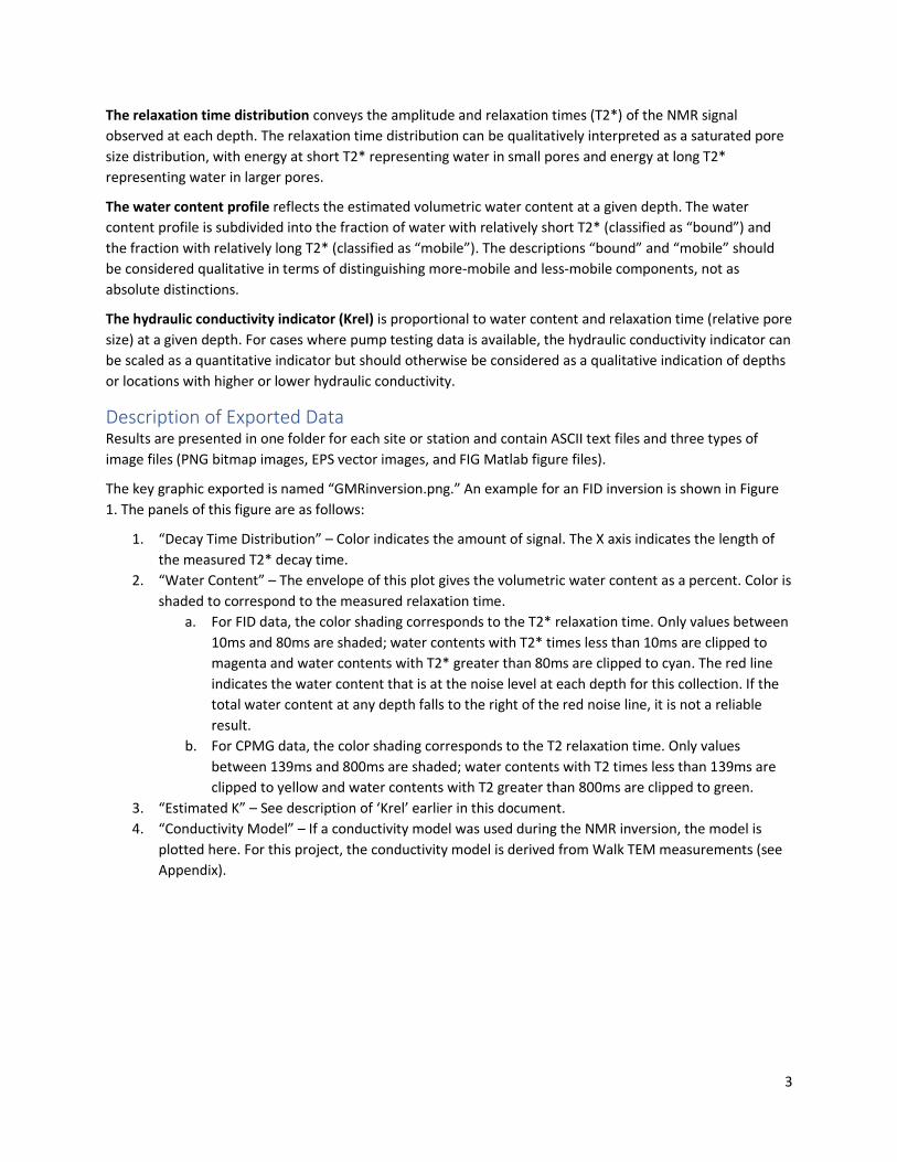
The key graphic exported is named “GMRinversion.png.” An example for an FID inversion is shown in Figure
1. The panels of this figure are as follows:
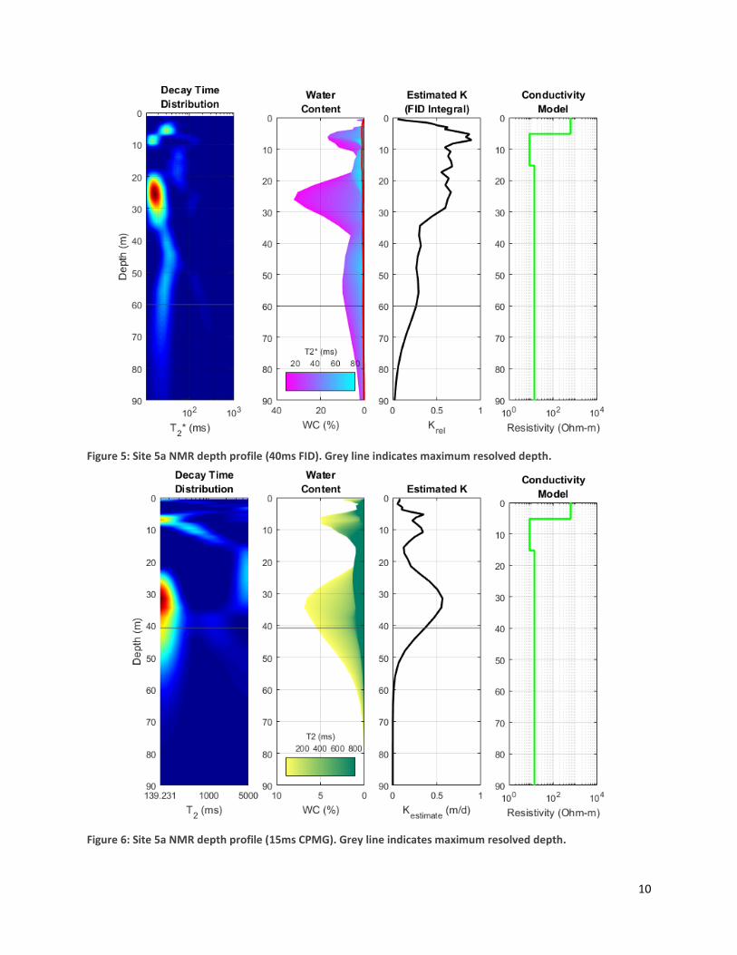
1. “Decay Time Distribution” – Color indicates the amount of signal. The X axis indicates the length of
the measured T2* decay time.
2. “Water Content” – The envelope of this plot gives the volumetric water content as a percent. Color is
shaded to correspond to the measured relaxation time.
a. For FID data, the color shading corresponds to the T2* relaxation time. Only values between
10ms and 80ms are shaded; water contents with T2* times less than 10ms are clipped to
magenta and water contents with T2* greater than 80ms are clipped to cyan. The red line
indicates the water content that is at the noise level at each depth for this collection. If the
total water content at any depth falls to the right of the red noise line, it is not a reliable
result.
b. For CPMG data, the color shading corresponds to the T2 relaxation time. Only values
between 139ms and 800ms are shaded; water contents with T2 times less than 139ms are
clipped to yellow and water contents with T2 greater than 800ms are clipped to green.
3. “Estimated K” – See description of ‘Krel’ earlier in this document.
4. “Conductivity Model” – If a conductivity model was used during the NMR inversion, the model is
plotted here. For this project, the conductivity model is derived from Walk TEM measurements (see
Appendix).
4
Figure 1: Example data product for an FID inversion.
Data Collection Between 9 and 13 November 2020, staff from Vista Clara and EKI made surface NMR soundings at 8 locations
(Table 1). Ramboll and Vista Clara made Walk TEM measurements at 6 sites, and Ramboll made Towed TEM
measurements at one site.
Table 1: Dates of GMR measurements and sites visited.
Date GMR Measurement
9-Nov Site 8
10-Nov Site 9
11-Nov Site 5a
11-Nov Site 7
12-Nov Site 11
12-Nov Site 2
13-Nov Site 3
13-Nov Site 10
Naming of GMR measurement sites followed EKI naming conventions.
5
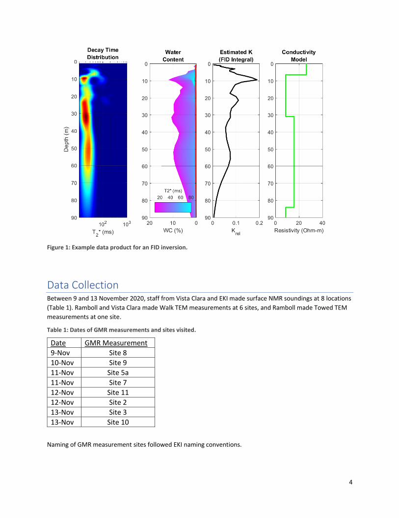
GPS waypoints were collected at each GMR measurement site (Figure 2), and these locations will be provided
as a Google Earth .KMZ file. For circular surface loops, a single GPS location indicates the center of the
measurement loop. For figure-eight surface loops, two GPS locations indicate the center of the two circles
that comprise the figure-eight.
Figure 2: GPS locations of GMR data collections. A Google Earth KMZ file of these locations is provided.
Survey Design NMR surface loops geometries were chosen to maximize depth of investigation while keeping environmental
interference to acceptable levels. (Larger, circular loops permit deeper investigation, but are more
susceptible to interference from noise sources. Smaller loops and figure-eight loops are more resistant to
environmental noise, at the cost of decreased depth of investigation.)
NMR acquisition pulse sequences were chosen to maximize depth of investigation, detection of water signals,
and characterization of site hydrogeologic conditions.
Most pulse sequences used in the project were Free Induction Decay (FID), which measures the apparent
relaxation time of the T2 NMR response (T2*). T2* is controlled by the pore size environment of the
measured fluids, but also by the presence of magnetic geology, which has the effect of decreasing the NMR
relaxation time, potentially causing fluids in large pores to present an NMR decay time similar to fluids in
small pores.
A second pulse sequence (CPMG) was used at sites with sufficiently high SNR (Sites 10 and 5a). The CPMG
sequence uses refocusing pulses to counter the effects of magnetic geology, potentially giving an indication
of the presence of mobile water in large pores that would not be indicated in an FID measurement.
At some sites, multiple FID measurements were made with different excitation pulse lengths: a longer pulse
length (e.g., 40 milliseconds) and a shorter pulse length (e.g., 15 milliseconds). Longer pulse moments allow
for excitation of water at greater depths, increasing the maximum depth of investigation, but surface NMR
measurements are unable to completely capture signals from fluids having a decay time shorter than or on
6
the order of the excitation pulse length, leading to a possible underrepresentation of total water content.
This underestimation is exacerbated by long excitation pulse lengths. Shorter excitation pulse lengths reduce
this effect but come with the tradeoff of decreasing the maximum depth of investigation.
The maximum sensitive depth of a surface NMR measurement is largely controlled by the size of the loop and
excitation pulse length but is also influenced by earth conductivity. If the subsurface has a relatively high
electrical resistivity, the depth of sensitivity can be the same as the loop diameter. If the electrical resistivity
is low, the depth of sensitivity will be reduced.
The areal sensitivity of a surface NMR measurement is roughly the area enclosed by the loop. That is, the
final 1-D depth profile represents an average over roughly the areal extent of the loop. Therefore, the depth
of investigation trades off with lateral resolution: investigation of deeper depths necessarily involves
averaging over larger lateral extents.
Equipment The equipment used was a Vista Clara GMR system manufactured, owned, and operated by Vista Clara. The
GMR is recognized as the most capable and sensitive surface NMR instrument on the market. It has a very
efficient power architecture, ultra-short dead-time to detect short signals, and very low noise floor to detect
small water volumes. The system also uses a multi-channel architecture that allows efficient noise
cancellation required to remove interference from cultural noise, such as powerlines, that can otherwise be
detrimental to NMR data.
The GMR equipment is deployed using two 12V deep cycle batteries and can be transported in off-highway
vehicles. A team of two operated the system, with typical operation consisting of deploying and retrieving
cable and monitoring data acquisition. Preliminary processing, inversion, and visualization of data is possible
in the field.
Data Processing Processing of raw NMR data and generation of depth profiles is done using Vista Clara's proprietary software.
Stacked data files are inverted for depth using an inversion algorithm that accounts for the loop geometry,
ambient magnetic field strength and orientation, and the pulse moments generated by the instrument.
Noise levels Power lines are typically the largest noise source for surface NMR surveys. Due to the spatial variability of
measurement sites in this project, every site presented a unique noise mitigation challenge. Some sites were
close to low voltage power lines, high-tension transmission lines, or radio transmitter towers.
There are several methods for mitigating the effects of environmental noise in surface NMR surveys,
including the use of smaller loops, figure-eight measurement coils, and reference loops. The multi-channel
design of the GMR makes it particularly effective at noise cancellation, which allowed for usable results at
sites that would otherwise not yield interpretable data.
Depth Sensitivity Depth sensitivity is modeled analytically during inversion. Depth sensitivity is a function of loop size,
excitation pulse length, and ground resistivity. For this survey, due to the variations in loop sizes and local
resistivities, depth sensitivity must be considered on a per-site basis. A depth resolution model is presented
for each inversion.
7
Conductivity model Depth sensitivity in surface NMR measurements is influenced by ground conductivity. The depth inversion
can take this effect into account by incorporating a layered conductivity model. This allows NMR energy to be
assigned in depth more accurately.
Inversions presented in this document were calculated incorporating layered conductivity models provided
by Walk TEM measurements. Some sites (9 and 11) did not have colocated TEM profiles and were inverted
using the conductivity profile from the nearest TEM site.
Inversion parameters All inversions shown have a dimensionless regularization parameter of suited to the SNR level of the data. A
correction is applied to all data to estimate and compensate for the NMR relaxation that occurs during the
transmit pulse.
Data Interpretation Interpretation of surface NMR data is dependent on-site conditions and signal characteristics. The following
factors should be considered in the interpretation of all data from the Cosumnes River project.
Magnetic geology Magnetic field inhomogeneity associated with magnetic geology can significantly influence the surface NMR
response. Vista Clara was able to confirm the influence of magnetic geology through data analysis and
specialized acquisition sequences. One indication of magnetic field inhomogeneity was the analyzed variation
in the NMR frequency between sites. The observed NMR frequency is directly proportional to the average
magnetic field at the site. Between Cosumnes River sites, the NMR frequency varied by more than 15Hz or
almost 1%. The influence of magnetic geology was also confirmed through the acquisition of patented CPMG
sequences and observation of an echo decay time T2 which is much longer than the FID decay time T2*.
Magnetic field inhomogeneity will influence the data in two ways. First, magnetic geology may result in some
underestimation of water content because a component of water in anomalous magnetic fields will not be
detected. Secondly, magnetic field inhomogeneity will shorten the FID decay time such that mobile water
with long T2 will exhibit a T2* closer to that of bound water. Zones of highly mobile water will not be as
readily distinguished in the FID or T2* distributions but will be highlighted in the CPMG echo signals and T2
results. Vista Clara conducted CPMG measurements at two sites with strong water signals, Site 5a and Site
10. The CPMG data are extremely valuable in that they confirm the T2 decay time is much longer than the
T2* decay time and highlight zones with particularly mobile water.
Influence of 2D/3D features In reviewing the data products, it is important to consider the lateral extent of the loops and the potential for
subsurface heterogeneity occurring at a smaller scale than the loop size. The data are inverted assuming a 1D
layered subsurface. Spatially constrained features such as a narrow channel or lens may have very high water
content within the feature (e.g. 30%), however, if the feature is small relative to the size of the loop (e.g. a
10m wide paleochannel in a 40m loop), the estimated water content will be scaled by the relative area of the
loop (e.g. <8%).
8
Layer Equivalence The vertical resolution of the surface NMR method is on the order of one meter near the surface and several
meters at the maximum depth of investigation. This resolution limit and the regularization of the inversion
results in a layer equivalence. A thin layer with high water content (e.g., a thickness of 1 m and water content
of 30%) will have an equivalent response to a thicker layer with a lower water content (e.g., a thickness of 3
m and water content of 10%). As such, low average water content values may be observed in a smoothed
inversion due to detected water being present as discrete layers below the resolution limit.
Bound Water Detection For the loop geometries and acquisition parameters (pulse lengths) used in this survey, it is not possible to
detect the fastest-decaying NMR signals associated with very bound water (i.e., water in clays). Detected
signals should therefore be assumed to reflect water associated with pores in silt or fine-fine sand. Zones
dominated by clay are most likely to be reflected as an absence of detected water.
Interpretation of Resistivity Profiles Electrical resistivity does not uniquely identify hydrogeologic characteristics and can be ambiguous to
interpret in the absence of other data. For example, low resistivity may be associated with impermeable clays
or with high permeability sands that are saturated with high TDS groundwater. In combination with surface
NMR data, the electrical resistivity can offer improved interpretation. Zones with low surface NMR water
detection and high resistivity would be consistent with unsaturated sands. Zones with low surface NMR
water detection and low resistivity would be consistent with clays. Zones with high surface NMR water
detection and high resistivity would be consistent with sands and low TDS pore fluid. Zones with high surface
NMR water detection and low resistivity would be consistent with sands and high TDS pore fluid.
Results Results are presented in order from highest signal-to-noise ratio (SNR) to lowest. Higher SNR means less
regularization is required in the inversion, allowing for finer depth resolution and greater confidence in the
results.
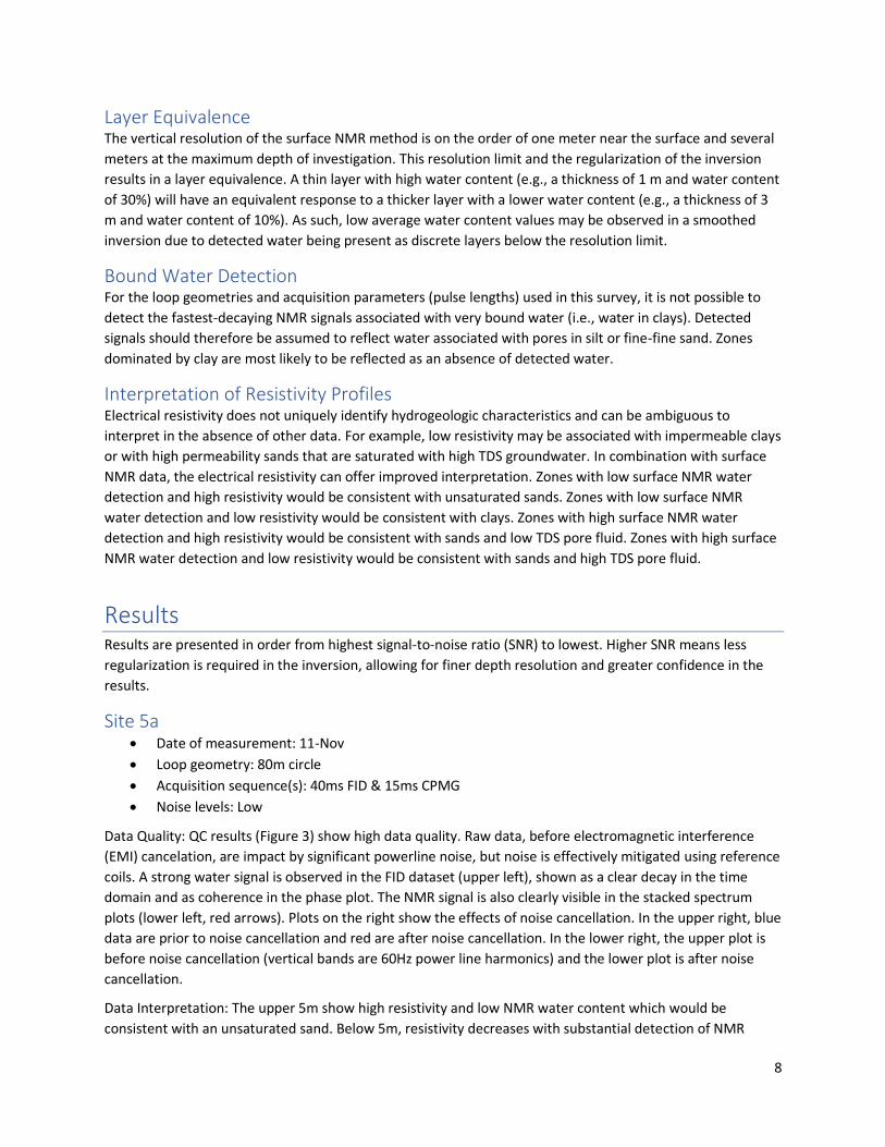
Site 5a • Date of measurement: 11-Nov
• Loop geometry: 80m circle
• Acquisition sequence(s): 40ms FID & 15ms CPMG
• Noise levels: Low
Data Quality: QC results (Figure 3) show high data quality. Raw data, before electromagnetic interference
(EMI) cancelation, are impact by significant powerline noise, but noise is effectively mitigated using reference
coils. A strong water signal is observed in the FID dataset (upper left), shown as a clear decay in the time
domain and as coherence in the phase plot. The NMR signal is also clearly visible in the stacked spectrum
plots (lower left, red arrows). Plots on the right show the effects of noise cancellation. In the upper right, blue
data are prior to noise cancellation and red are after noise cancellation. In the lower right, the upper plot is
before noise cancellation (vertical bands are 60Hz power line harmonics) and the lower plot is after noise
cancellation.
Data Interpretation: The upper 5m show high resistivity and low NMR water content which would be
consistent with an unsaturated sand. Below 5m, resistivity decreases with substantial detection of NMR
9
water, which would be consistent with the presence of permeable sands and possibly high TDS. Zones with
especially mobile water are highlighted by relatively long T2* values and long T2 values from the CPMG data.
Figure 3: Quality Control (QC) results for Site 5a (40ms FID).
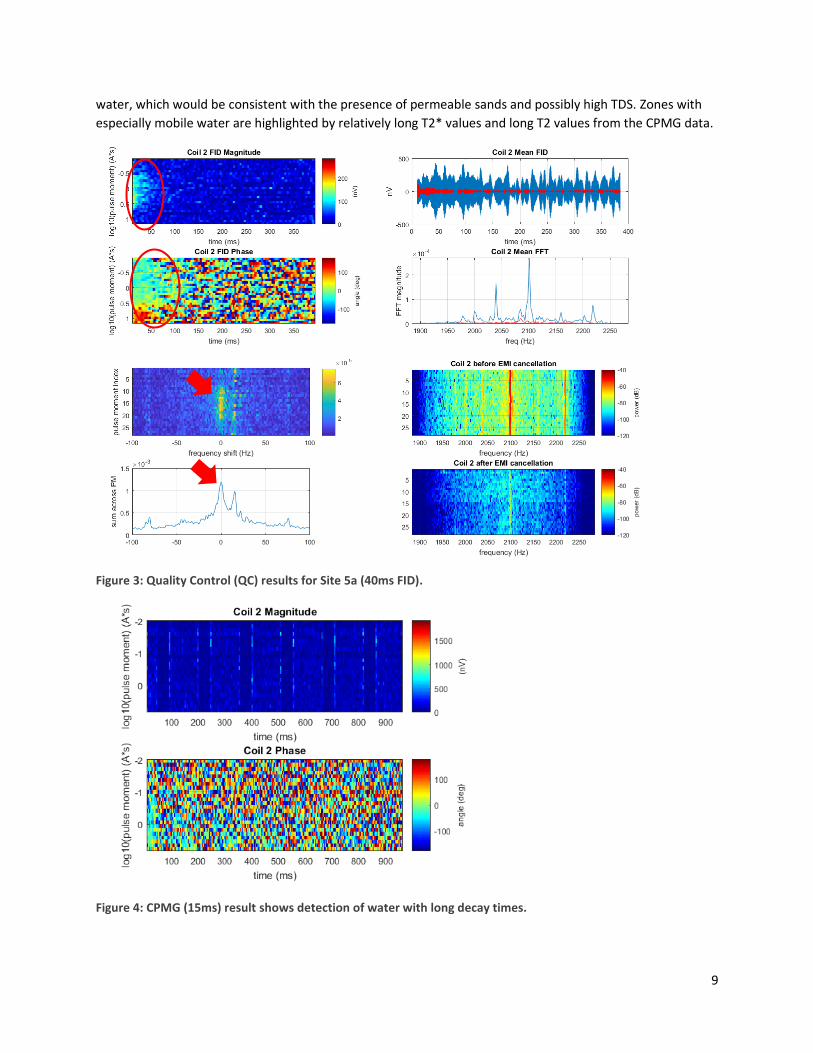
Figure 4: CPMG (15ms) result shows detection of water with long decay times.
10
Figure 5: Site 5a NMR depth profile (40ms FID). Grey line indicates maximum resolved depth.
Figure 6: Site 5a NMR depth profile (15ms CPMG). Grey line indicates maximum resolved depth.
11
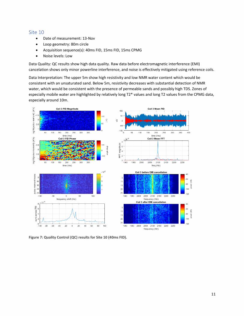
Site 10 • Date of measurement: 13-Nov
• Loop geometry: 80m circle
• Acquisition sequence(s): 40ms FID, 15ms FID, 15ms CPMG
• Noise levels: Low
Data Quality: QC results show high data quality. Raw data before electromagnetic interference (EMI)
cancelation shows only minor powerline interference, and noise is effectively mitigated using reference coils.
Data Interpretation: The upper 5m show high resistivity and low NMR water content which would be
consistent with an unsaturated sand. Below 5m, resistivity decreases with substantial detection of NMR
water, which would be consistent with the presence of permeable sands and possibly high TDS. Zones of
especially mobile water are highlighted by relatively long T2* values and long T2 values from the CPMG data,
especially around 10m.
Figure 7: Quality Control (QC) results for Site 10 (40ms FID).
12
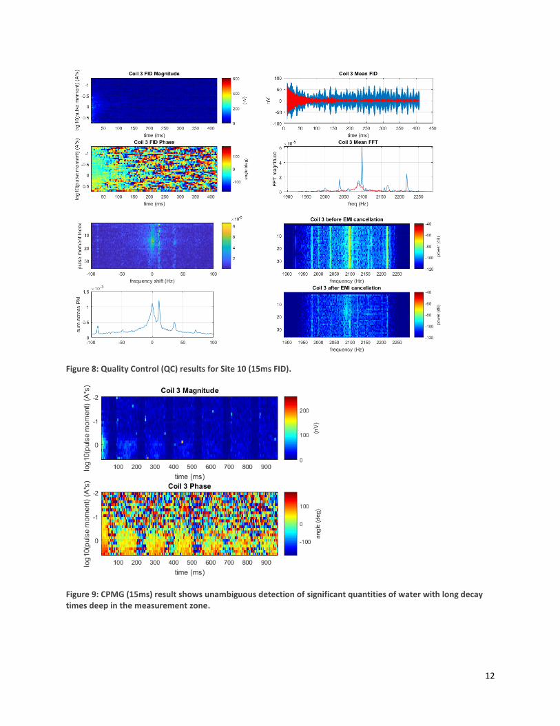
Figure 8: Quality Control (QC) results for Site 10 (15ms FID).
Figure 9: CPMG (15ms) result shows unambiguous detection of significant quantities of water with long decay times deep in the measurement zone.
13
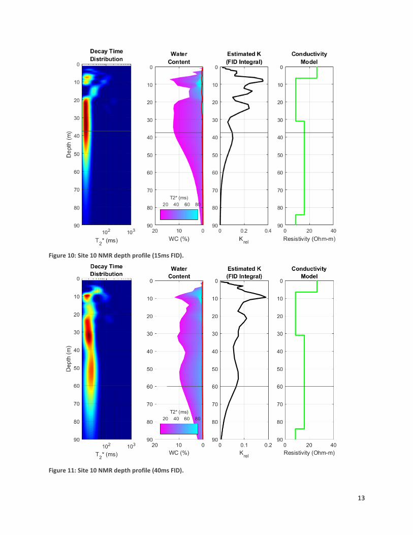
Figure 10: Site 10 NMR depth profile (15ms FID).
Figure 11: Site 10 NMR depth profile (40ms FID).
14
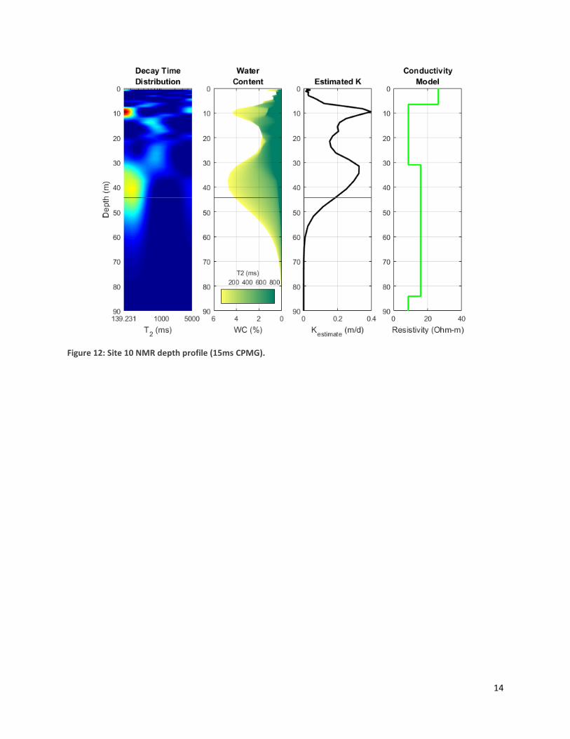
Figure 12: Site 10 NMR depth profile (15ms CPMG).
15
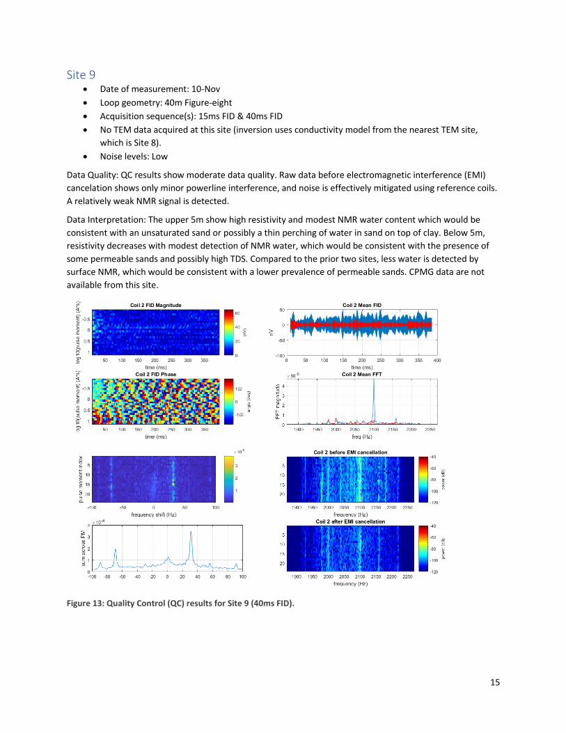
Site 9 • Date of measurement: 10-Nov
• Loop geometry: 40m Figure-eight
• Acquisition sequence(s): 15ms FID & 40ms FID
• No TEM data acquired at this site (inversion uses conductivity model from the nearest TEM site,
which is Site 8).
• Noise levels: Low
Data Quality: QC results show moderate data quality. Raw data before electromagnetic interference (EMI)
cancelation shows only minor powerline interference, and noise is effectively mitigated using reference coils.
A relatively weak NMR signal is detected.
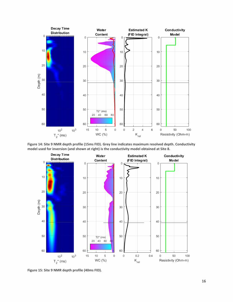
Data Interpretation: The upper 5m show high resistivity and modest NMR water content which would be
consistent with an unsaturated sand or possibly a thin perching of water in sand on top of clay. Below 5m,
resistivity decreases with modest detection of NMR water, which would be consistent with the presence of
some permeable sands and possibly high TDS. Compared to the prior two sites, less water is detected by
surface NMR, which would be consistent with a lower prevalence of permeable sands. CPMG data are not
available from this site.
Figure 13: Quality Control (QC) results for Site 9 (40ms FID).
16
Figure 14: Site 9 NMR depth profile (15ms FID). Grey line indicates maximum resolved depth. Conductivity model used for inversion (and shown at right) is the conductivity model obtained at Site 8.
Figure 15: Site 9 NMR depth profile (40ms FID).
17
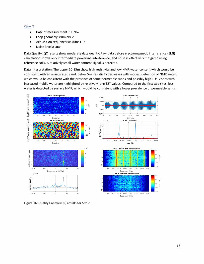
Site 7 • Date of measurement: 11-Nov
• Loop geometry: 80m circle
• Acquisition sequence(s): 40ms FID
• Noise levels: Low
Data Quality: QC results show moderate data quality. Raw data before electromagnetic interference (EMI)
cancelation shows only intermediate powerline interference, and noise is effectively mitigated using
reference coils. A relatively small water content signal is detected.
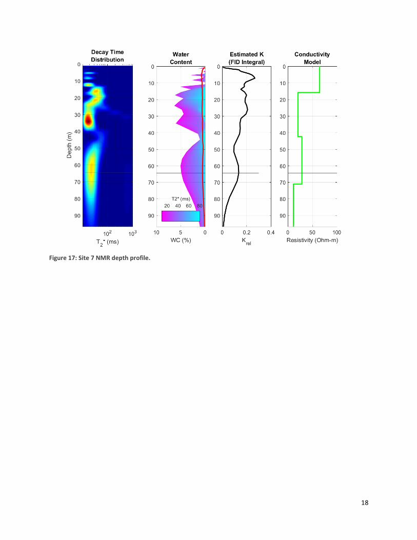
Data Interpretation: The upper 10-15m show high resistivity and low NMR water content which would be
consistent with an unsaturated sand. Below 5m, resistivity decreases with modest detection of NMR water,
which would be consistent with the presence of some permeable sands and possibly high TDS. Zones with
increased mobile water are highlighted by relatively long T2* values. Compared to the first two sites, less
water is detected by surface NMR, which would be consistent with a lower prevalence of permeable sands.
Figure 16: Quality Control (QC) results for Site 7.
18
Figure 17: Site 7 NMR depth profile.
19
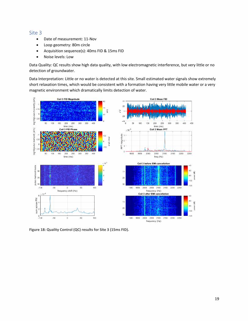
Site 3 • Date of measurement: 11-Nov
• Loop geometry: 80m circle
• Acquisition sequence(s): 40ms FID & 15ms FID
• Noise levels: Low
Data Quality: QC results show high data quality, with low electromagnetic interference, but very little or no
detection of groundwater.
Data Interpretation: Little or no water is detected at this site. Small estimated water signals show extremely
short relaxation times, which would be consistent with a formation having very little mobile water or a very
magnetic environment which dramatically limits detection of water.
Figure 18: Quality Control (QC) results for Site 3 (15ms FID).
20
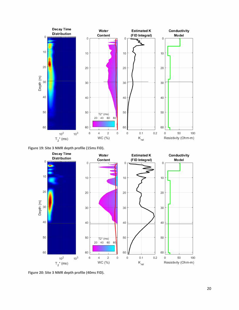
Figure 19: Site 3 NMR depth profile (15ms FID).
Figure 20: Site 3 NMR depth profile (40ms FID).
21
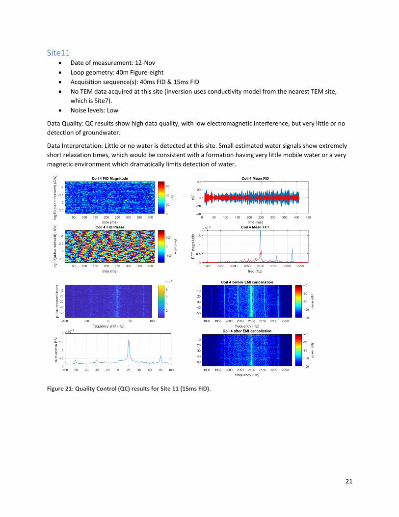
Site11 • Date of measurement: 12-Nov
• Loop geometry: 40m Figure-eight
• Acquisition sequence(s): 40ms FID & 15ms FID
• No TEM data acquired at this site (inversion uses conductivity model from the nearest TEM site,
which is Site7).
• Noise levels: Low
Data Quality: QC results show high data quality, with low electromagnetic interference, but very little or no
detection of groundwater.
Data Interpretation: Little or no water is detected at this site. Small estimated water signals show extremely
short relaxation times, which would be consistent with a formation having very little mobile water or a very
magnetic environment which dramatically limits detection of water.
Figure 21: Quality Control (QC) results for Site 11 (15ms FID).
22
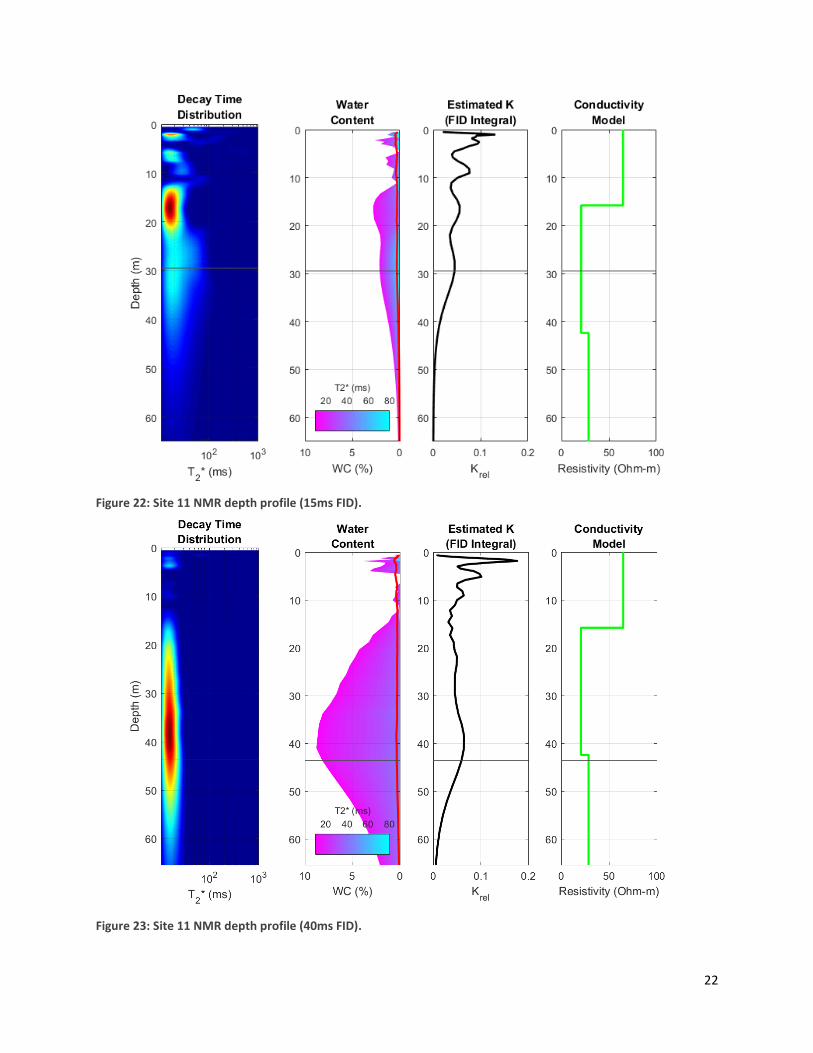
Figure 22: Site 11 NMR depth profile (15ms FID).
Figure 23: Site 11 NMR depth profile (40ms FID).
23
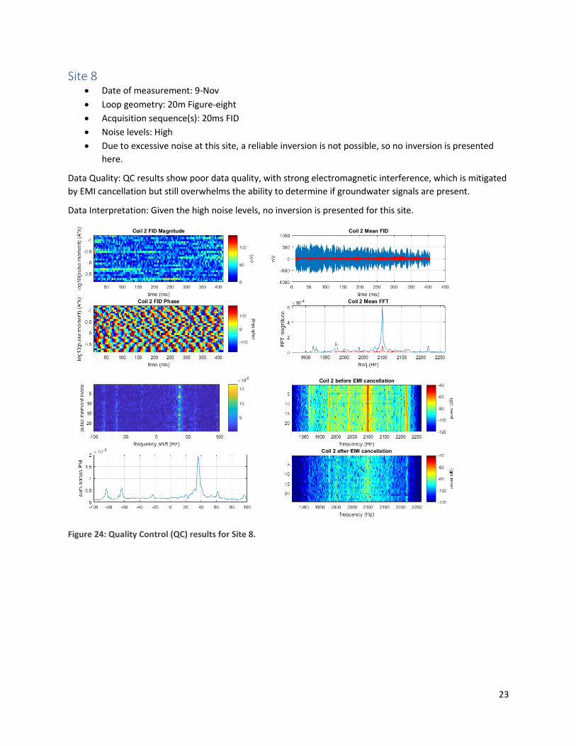
Site 8 • Date of measurement: 9-Nov
• Loop geometry: 20m Figure-eight
• Acquisition sequence(s): 20ms FID
• Noise levels: High
• Due to excessive noise at this site, a reliable inversion is not possible, so no inversion is presented
here.
Data Quality: QC results show poor data quality, with strong electromagnetic interference, which is mitigated
by EMI cancellation but still overwhelms the ability to determine if groundwater signals are present.
Data Interpretation: Given the high noise levels, no inversion is presented for this site.
Figure 24: Quality Control (QC) results for Site 8.
24
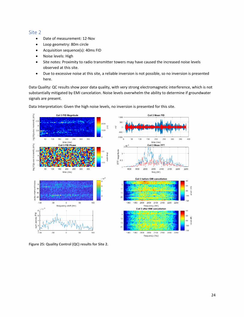
Site 2 • Date of measurement: 12-Nov
• Loop geometry: 80m circle
• Acquisition sequence(s): 40ms FID
• Noise levels: High
• Site notes: Proximity to radio transmitter towers may have caused the increased noise levels
observed at this site.
• Due to excessive noise at this site, a reliable inversion is not possible, so no inversion is presented
here.
Data Quality: QC results show poor data quality, with very strong electromagnetic interference, which is not
substantially mitigated by EMI cancelation. Noise levels overwhelm the ability to determine if groundwater
signals are present.
Data Interpretation: Given the high noise levels, no inversion is presented for this site.
Figure 25: Quality Control (QC) results for Site 2.
25
Appendix
Exported Data Format for Surface NMR Data The ASCII text files associated with the exported inversion have the suffix “_1d_inversion.txt.” The format of
first 11 columns of these files is as follows:
Column 1: Upper boundary of layer (m)
Column 2: Lower boundary of layer (m)
Column 3: Relative permeability (Krel), estimated as squared integral of demodulated FID signal
Column 4: Water content (fraction of 1.0)
Column 5: T2* (s) [for FID data] or T2 (s) [for spin echo or CPMG data]
Column 6: Frequency (Hz)
Column 7: Phase (radians)
Column 8: T1 (s) [for T1 dataset] or NaN [for all other datasets]
Column 9: Bound water content
Column 10: Mobile water content
Column 11: Total water content
The remaining columns contain inverted amplitude values for the multi-exponential distributions for the
same depth levels corresponding to column 1 and column 2. The last row of the file contains the decay time
values (in seconds) for each of the amplitudes values in the correspond column.
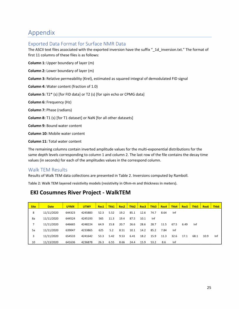
Walk TEM Results Results of Walk TEM data collections are presented in Table 2. Inversions computed by Ramboll.
Table 2: Walk TEM layered resistivity models (resistivity in Ohm-m and thickness in meters).
EKI Cosumnes River Project - WalkTEM
Site Date UYMX UTMY Res1 Thk1 Res2 Thk2 Res3 Thk3 Res4 Thk4 Res5 Thk5 Res6 Thk6
8 11/11/2020 644323 4245883 52.3 5.52 19.2 85.1 12.6 74.7 8.64 Inf
8a 11/11/2020 644524 4245193 565 11.3 19.4 87.5 10.1 Inf
7 11/11/2020 646665 4248224 64.9 15.8 20.7 26.6 28.6 28.7 11.5 67.5 6.49 Inf
5a 11/11/2020 639047 4233865 625 5.2 8.51 10.1 14.2 85.2 7.84 Inf
3 11/11/2020 654533 4241642 53.3 5.42 9.53 6.41 18.2 15.9 11.3 32.6 17.1 68.1 10.9 Inf
10 11/13/2020 641636 4236878 26.3 6.55 8.66 24.4 15.9 53.2 8.6 Inf