Surface Runoff: A Rainfall Simulator For Wash-Off …...Surface Runoff: A Rainfall Simulator For Wash-Off Modelling And Road Safety Auditing Under Different Rainfall Intensities Simone

Surface Runoff: A Rainfall Simulator For Wash-Off Modelling And Road Safety

Auditing Under Different Rainfall Intensities

Simone A. Professor – University of Bologna – DISTART Strade Vignali V. Ph.D Student – University of Bologna – DISTART Strade Bragalli C. Researcher – University of Bologna – DISTART Costruzioni Idrauliche Maglionico M. Researcher – University of Bologna – DISTART Costruzioni Idrauliche

SYNOPSIS The great traffic and vehicle average speed increase in recent years have improved road pavements performance standards. Road surface must be designed, built and maintained to offer the highest active safety to drivers. This is very important during rainfall events, because the water collected on road pavements produces a drastic decrease of skid resistance and visual distance. So water film depth estimation is one of the most important factor on road safety. Moreover during rainfall events the rainfall wash pollutants collected on road pavements and dissolve them in urban drainage with an important environmental impact. In this paper has been studied and modelled the pollutants wash-off on road pavements and the vehicle-road interaction in terms of water film depth. The laboratory equipment consists of an artificial rain system, capable of simulating variable rainfall intensities by different nozzles and by a controlled water discharge system to collect the water flowing from the road surface. To reproduce different rainfall intensities, three nozzles were used and calibrated according to rainfall intensity, drop dimension distribution and medium drop diameter. From rated flow calculation it has been investigated: the effect of different rainfall intensity regimes on pollutants wash-off and safety; the effect of different surface slope on wash-off and safety; the effect of water film depth on skid resistance and safety.

The data collected in this way have been submitted to an in-depth analysis, which has provided particularly interesting and significant results regarding design and maintenance of roads according to security and environmental standards.

Surface Runoff: A Rainfall Simulator For Wash-Off Modelling And Road Safety

Auditing Under Different Rainfall Intensities

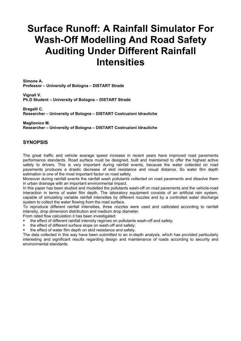
INTRODUCTION The rainfall events on an asphalt surface produce two different effects: the first on the water film, and consequently on road safety, and the other on the road waste runoff, which is directly connected to the environmental impact. In this paper has been studied and modelled the pollutants wash-off on road pavements and the vehicle-road interaction in terms of water film depth. An understanding of pollutant wash-off characteristics is essential to estimate and to minimise the impacts of pollutants on the environment. Stormwater quality models typically view stormwater pollution as a two stage process, pollutant build-up and pollutant wash-off. Build-up is the accumulation of pollutants on the catchment surface during dry periods and wash-off is the removal of the pollutants by rainfall and runoff (Vaze and Chiew, 2002). The few studies on pollutant build-up, since the detailed experimental pollutant accumulation studies of Sartor and Boyd in 1972, agree that surface pollutant load increase during antecedent dry weather period, but there are doubts on the assumption that the buildup starts from zero after a rain event is realistic. Depending on the rainfall and runoff characteristics, part of the available pollutant is removed from the surface as wash-off, the remainder becomes a part of the fixed load as it attaches itself to the surface. During drying, part of the free load of the build-up process can attach itself to the surface contributing to the fixed load amount. The experimental study on an urban road surface in Melbourne (Vaze and Chiew, 2002) has shown that common storms only remove a small proportion of the total surface pollutant load, also it has suggested that the rainfall and runoff disintegrate and dissolve more surface pollutant that they can actually remove. The road surface conditions and temperature are very important for the adherence values. In real conditions the road could be contaminated with dust, mud or sand, or covered with water, ice or snow. On the wet roads, when the water thickness is very low and motor vehicle speed in normal range, it could be observed a somewhat decrease of adherence. This fact could be explain due to the diminish value of adhesion friction on lubricated surfaces. The peak and slide values of the longitudinal force coefficient on wet road compared to the values on dry road are presented in figure 1.

Figure 1: Comparison between dry and wet road adherence conditions [Pauwelussen, 2002]

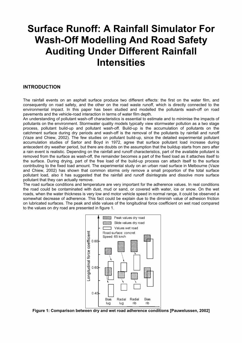
In addition, the influences of load and vehicles speed are depicted in figure 2.

Figure 2: Comparison of load and speed effect on dry and wet roads (radial truck tyre) [Pauwelussen,

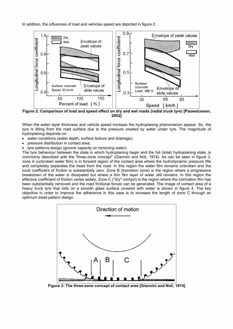
2002] When the water layer thickness and vehicle speed increase the hydroplaning phenomenon appear. So, the tyre is lifting from the road surface due to the pressure created by water under tyre. The magnitude of hydroplaning depends on: • water conditions (water depth, surface texture and drainage); • pressure distribution in contact area; • tyre patterns design (groove capacity on removing water). The tyre behaviour between the state in which hydroplaning begin and the full (total) hydroplaning state, is commonly described with the "three-zone concept" (Giannini and Noli, 1974). As can be seen in figure 3, zone A (unbroken water film) is in forward region of the contact area where the hydrodynamic pressure lifts and completely separates the tread from the road. In this region the water film remains unbroken and the local coefficient of friction is substantially zero. Zone B (transition zone) is the region where a progressive breakdown of the water is dissipated but where a thin film layer of water still remains. In this region the effective coefficient of friction varies widely. Zone C ("dry" contact) is the region where the lubrication film has been substantially removed and the road frictional forces can be generated. The image of contact area of a heavy truck tyre that rolls on a smooth glass surface covered with water is shown in figure 4. The key objective in order to improve the adherence in this case is to increase the length of zone C through an optimum tread pattern design.

Figure 3: The three-zone concept of contact area [Giannini and Noli, 1974]

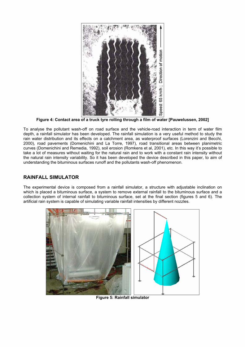
Figure 4: Contact area of a truck tyre rolling through a film of water [Pauwelussen, 2002]

To analyse the pollutant wash-off on road surface and the vehicle-road interaction in term of water film depth, a rainfall simulator has been developed. The rainfall simulation is a very useful method to study the rain water distribution and its effects on a catchment area, as waterproof surfaces (Lorenzini and Becchi, 2000), road pavements (Domenichini and La Torre, 1997), road transitional areas between planimetric curves (Domenichini and Remedia, 1992), soil erosion (Romkens et al, 2001), etc. In this way it’s possible to take a lot of measures without waiting for the natural rain and to work with a constant rain intensity without the natural rain intensity variability. So it has been developed the device described in this paper, to aim of understanding the bituminous surfaces runoff and the pollutants wash-off phenomenon.

RAINFALL SIMULATOR The experimental device is composed from a rainfall simulator, a structure with adjustable inclination on which is placed a bituminous surface, a system to remove external rainfall to the bituminous surface and a collection system of internal rainfall to bituminous surface, set at the final section (figures 5 and 6). The artificial rain system is capable of simulating variable rainfall intensities by different nozzles.

Figure 5: Rainfall simulator

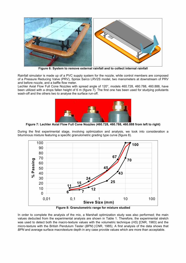
Figure 6: System to remove external rainfall and to collect internal rainfall

Rainfall simulator is made up of a PVC supply system for the nozzle, while control members are composed of a Pressure Reducing Valve (PRV), Spirax Sarco LRV2S model, two manometers at downstream of PRV and before nozzle, and a baffle flow meter. Lechler Axial Flow Full Cone Nozzles with spread angle of 120°, models 460.728, 460.788, 460.888, have been utilized with a drops fallen height of 6 m (figure 7). The first one has been used for studying pollutants wash-off and the others two to analyse the surface run-off.

Figure 7: Lechler Axial Flow Full Cone Nozzles (460.728, 460.788, 460.888 from left to right)

During the first experimental stage, involving optimization and analysis, we took into consideration a bituminous mixture featuring a specific granulometric grading type curve (figure 8).

1276

25

43

70

45

67

24

1115

100

0102030405060708090

100

0,01 0,1 1 10 100Sieve Size (mm)

% P

assi

ng

Figure 8: Granulometric range for mixture studied

In order to complete the analysis of the mix, a Marshall optimization study was also performed; the main values deducted from the experimental analysis are shown in Table 1. Therefore, the experimental stretch was used to detect both the macro-texture values with the volumetric technique (HS) [CNR, 1983] and the micro-texture with the British Pendulum Tester (BPN) [CNR, 1985]. A first analysis of the data shows that BPN and average surface macrotexture depth in any case provide values which are more than acceptable.

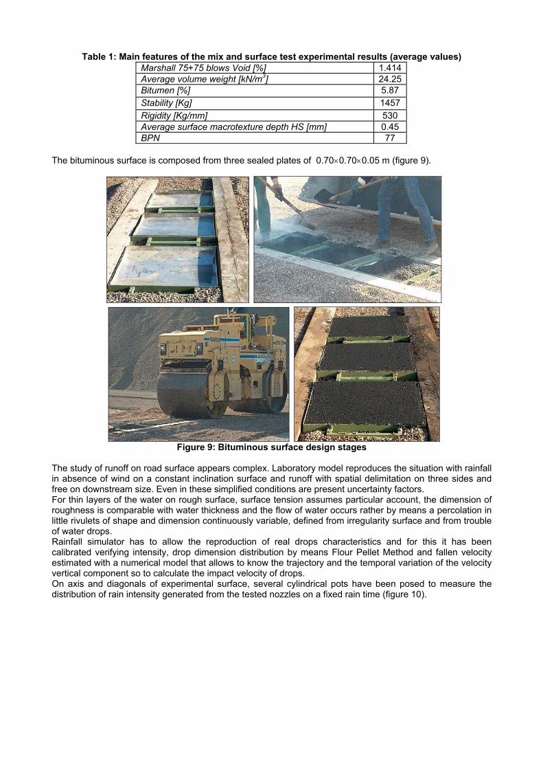
Table 1: Main features of the mix and surface test experimental results (average values) Marshall 75+75 blows Void [%] 1.414 Average volume weight [kN/m3] 24.25 Bitumen [%] 5.87 Stability [Kg] 1457 Rigidity [Kg/mm] 530 Average surface macrotexture depth HS [mm] 0.45 BPN 77

The bituminous surface is composed from three sealed plates of 0.70×0.70×0.05 m (figure 9).

Figure 9: Bituminous surface design stages

The study of runoff on road surface appears complex. Laboratory model reproduces the situation with rainfall in absence of wind on a constant inclination surface and runoff with spatial delimitation on three sides and free on downstream size. Even in these simplified conditions are present uncertainty factors. For thin layers of the water on rough surface, surface tension assumes particular account, the dimension of roughness is comparable with water thickness and the flow of water occurs rather by means a percolation in little rivulets of shape and dimension continuously variable, defined from irregularity surface and from trouble of water drops. Rainfall simulator has to allow the reproduction of real drops characteristics and for this it has been calibrated verifying intensity, drop dimension distribution by means Flour Pellet Method and fallen velocity estimated with a numerical model that allows to know the trajectory and the temporal variation of the velocity vertical component so to calculate the impact velocity of drops. On axis and diagonals of experimental surface, several cylindrical pots have been posed to measure the distribution of rain intensity generated from the tested nozzles on a fixed rain time (figure 10).

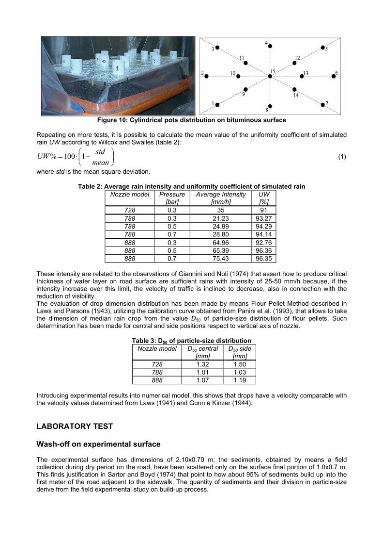
Figure 10: Cylindrical pots distribution on bituminous surface

Repeating on more tests, it is possible to calculate the mean value of the uniformity coefficient of simulated rain UW according to Wilcox and Swailes (table 2):

−⋅=

meanstdUW 1100% (1)

where std is the mean square deviation.

Table 2: Average rain intensity and uniformity coefficient of simulated rain Nozzle model Pressure

[bar] Average Intensity

[mm/h] UW [%]

728 0.3 35 91 788 0.3 21.23 93.27 788 0.5 24.99 94.29 788 0.7 28.80 94.14 888 0.3 64.96 92.76 888 0.5 65.39 96.36 888 0.7 75.43 96.35

These intensity are related to the observations of Giannini and Noli (1974) that assert how to produce critical thickness of water layer on road surface are sufficient rains with intensity of 25-50 mm/h because, if the intensity increase over this limit, the velocity of traffic is inclined to decrease, also in connection with the reduction of visibility. The evaluation of drop dimension distribution has been made by means Flour Pellet Method described in Laws and Parsons (1943), utilizing the calibration curve obtained from Panini et al. (1993), that allows to take the dimension of median rain drop from the value D50 of particle-size distribution of flour pellets. Such determination has been made for central and side positions respect to vertical axis of nozzle.

Table 3: D50 of particle-size distribution Nozzle model D50 central

[mm] D50 side

[mm] 728 1.32 1.50 788 1.01 1.03 888 1.07 1.19

Introducing experimental results into numerical model, this shows that drops have a velocity comparable with the velocity values determined from Laws (1941) and Gunn e Kinzer (1944).

LABORATORY TEST Wash-off on experimental surface The experimental surface has dimensions of 2.10x0.70 m; the sediments, obtained by means a field collection during dry period on the road, have been scattered only on the surface final portion of 1.0x0.7 m. This finds justification in Sartor and Boyd (1974) that point to how about 95% of sediments build up into the first meter of the road adjacent to the sidewalk. The quantity of sediments and their division in particle-size derive from the field experimental study on build-up process.

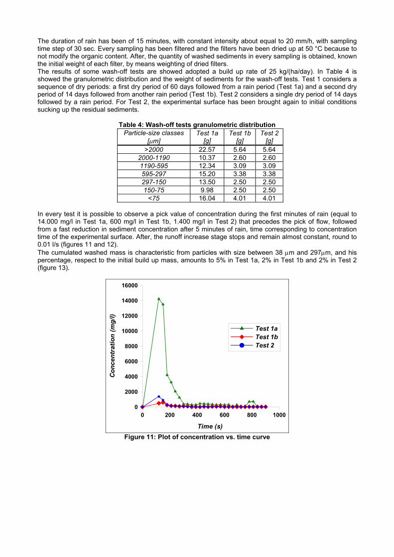
The duration of rain has been of 15 minutes, with constant intensity about equal to 20 mm/h, with sampling time step of 30 sec. Every sampling has been filtered and the filters have been dried up at 50 °C because to not modify the organic content. After, the quantity of washed sediments in every sampling is obtained, known the initial weight of each filter, by means weighting of dried filters. The results of some wash-off tests are showed adopted a build up rate of 25 kg/(ha/day). In Table 4 is showed the granulometric distribution and the weight of sediments for the wash-off tests. Test 1 considers a sequence of dry periods: a first dry period of 60 days followed from a rain period (Test 1a) and a second dry period of 14 days followed from another rain period (Test 1b). Test 2 considers a single dry period of 14 days followed by a rain period. For Test 2, the experimental surface has been brought again to initial conditions sucking up the residual sediments.

Table 4: Wash-off tests granulometric distribution Particle-size classes

[µm] Test 1a

[g] Test 1b

[g] Test 2

[g] >2000 22.57 5.64 5.64

2000-1190 10.37 2.60 2.60 1190-595 12.34 3.09 3.09 595-297 15.20 3.38 3.38 297-150 13.50 2.50 2.50 150-75 9.98 2.50 2.50

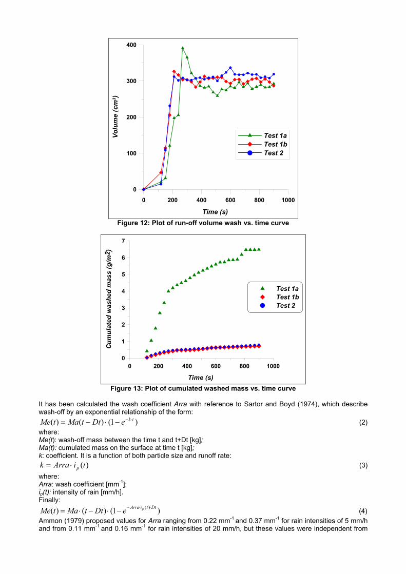
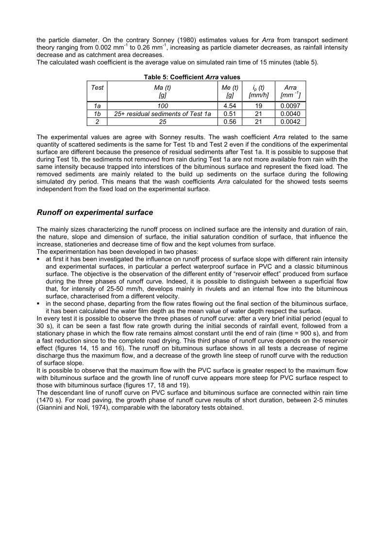
<75 16.04 4.01 4.01 In every test it is possible to observe a pick value of concentration during the first minutes of rain (equal to 14.000 mg/l in Test 1a, 600 mg/l in Test 1b, 1.400 mg/l in Test 2) that precedes the pick of flow, followed from a fast reduction in sediment concentration after 5 minutes of rain, time corresponding to concentration time of the experimental surface. After, the runoff increase stage stops and remain almost constant, round to 0.01 l/s (figures 11 and 12). The cumulated washed mass is characteristic from particles with size between 38 µm and 297µm, and his percentage, respect to the initial build up mass, amounts to 5% in Test 1a, 2% in Test 1b and 2% in Test 2 (figure 13).

0 200 400 600 800 1000

Time (s)

0

4000

8000

12000

16000

2000

6000

10000

14000

Con

cent

ratio

n (m

g/l)

Test 1aTest 1bTest 2

Figure 11: Plot of concentration vs. time curve

0 200 400 600 800 1000

Time (s)

0

100

200

300

400

Volu

me

(cm

3 )


Figure 12: Plot of run-off volume wash vs. time curve

0 200 400 600 800 1000

Time (s)

0

1

2

3

4

5

6

7

Cum

ulat

ed w

ashe

d m

ass

(g/m

2 )


Figure 13: Plot of cumulated washed mass vs. time curve

It has been calculated the wash coefficient Arra with reference to Sartor and Boyd (1974), which describe wash-off by an exponential relationship of the form:

)1()()( tkeDttMatMe ⋅−−⋅−= (2) where: Me(t): wash-off mass between the time t and t+Dt [kg]; Ma(t): cumulated mass on the surface at time t [kg]; k: coefficient. It is a function of both particle size and runoff rate:

)(tiArrak p⋅= (3) where: Arra: wash coefficient [mm-1]; ip(t): intensity of rain [mm/h]. Finally:

)1()()( )( DttiArra peDttMatMe ⋅⋅−−⋅−⋅= (4) Ammon (1979) proposed values for Arra ranging from 0.22 mm-1 and 0.37 mm-1 for rain intensities of 5 mm/h and from 0.11 mm-1 and 0.16 mm-1 for rain intensities of 20 mm/h, but these values were independent from

the particle diameter. On the contrary Sonney (1980) estimates values for Arra from transport sediment theory ranging from 0.002 mm-1 to 0.26 mm-1, increasing as particle diameter decreases, as rainfall intensity decrease and as catchment area decreases. The calculated wash coefficient is the average value on simulated rain time of 15 minutes (table 5).

Table 5: Coefficient Arra values Test

Ma (t)

[g] Me (t)

[g] ip (t)

[mm/h] Arra

[mm -1]

1a 100 4.54 19 0.0097 1b 25+ residual sediments of Test 1a 0.51 21 0.0040 2 25 0.56 21 0.0042

The experimental values are agree with Sonney results. The wash coefficient Arra related to the same quantity of scattered sediments is the same for Test 1b and Test 2 even if the conditions of the experimental surface are different because the presence of residual sediments after Test 1a. It is possible to suppose that during Test 1b, the sediments not removed from rain during Test 1a are not more available from rain with the same intensity because trapped into interstices of the bituminous surface and represent the fixed load. The removed sediments are mainly related to the build up sediments on the surface during the following simulated dry period. This means that the wash coefficients Arra calculated for the showed tests seems independent from the fixed load on the experimental surface.

Runoff on experimental surface The mainly sizes characterizing the runoff process on inclined surface are the intensity and duration of rain, the nature, slope and dimension of surface, the initial saturation condition of surface, that influence the increase, stationeries and decrease time of flow and the kept volumes from surface. The experimentation has been developed in two phases: at first it has been investigated the influence on runoff process of surface slope with different rain intensity

and experimental surfaces, in particular a perfect waterproof surface in PVC and a classic bituminous surface. The objective is the observation of the different entity of “reservoir effect” produced from surface during the three phases of runoff curve. Indeed, it is possible to distinguish between a superficial flow that, for intensity of 25-50 mm/h, develops mainly in rivulets and an internal flow into the bituminous surface, characterised from a different velocity.

in the second phase, departing from the flow rates flowing out the final section of the bituminous surface, it has been calculated the water film depth as the mean value of water depth respect the surface.

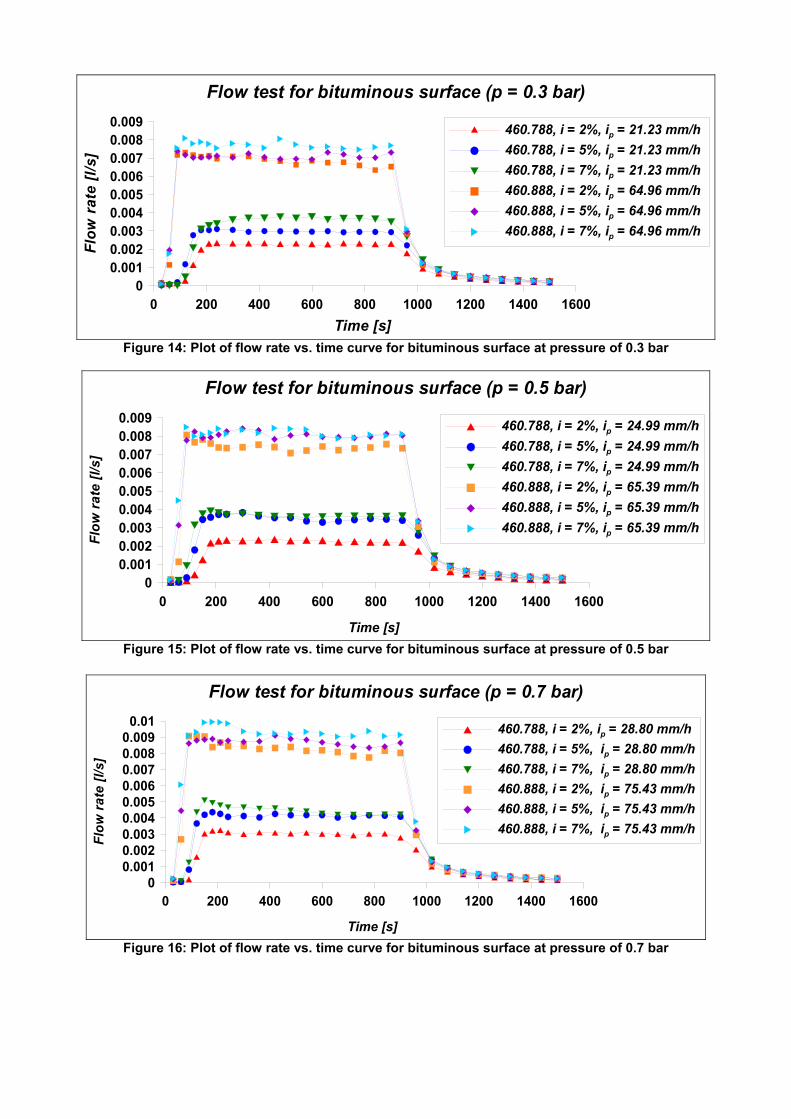
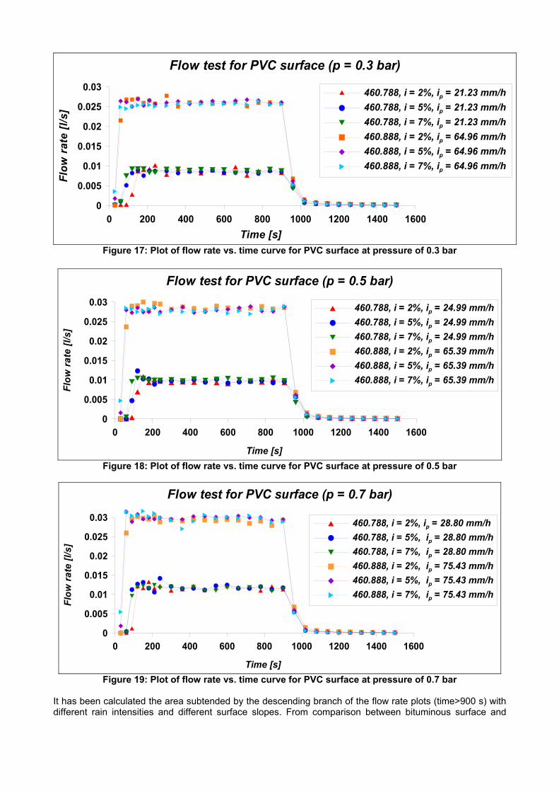
In every test it is possible to observe the three phases of runoff curve: after a very brief initial period (equal to 30 s), it can be seen a fast flow rate growth during the initial seconds of rainfall event, followed from a stationary phase in which the flow rate remains almost constant until the end of rain (time = 900 s), and from a fast reduction since to the complete road drying. This third phase of runoff curve depends on the reservoir effect (figures 14, 15 and 16). The runoff on bituminous surface shows in all tests a decrease of regime discharge thus the maximum flow, and a decrease of the growth line steep of runoff curve with the reduction of surface slope. It is possible to observe that the maximum flow with the PVC surface is greater respect to the maximum flow with bituminous surface and the growth line of runoff curve appears more steep for PVC surface respect to those with bituminous surface (figures 17, 18 and 19). The descendant line of runoff curve on PVC surface and bituminous surface are connected within rain time (1470 s). For road paving, the growth phase of runoff curve results of short duration, between 2-5 minutes (Giannini and Noli, 1974), comparable with the laboratory tests obtained.

0 400 800 1200 1600200 600 1000 1400Time [s]

0

0.002

0.004

0.006

0.008

0.001

0.003

0.005

0.007

0.009

Flow

rat

e [l/

s]

460.788, i = 2%, ip = 21.23 mm/h 460.788, i = 5%, ip = 21.23 mm/h460.788, i = 7%, ip = 21.23 mm/h460.888, i = 2%, ip = 64.96 mm/h460.888, i = 5%, ip = 64.96 mm/h460.888, i = 7%, ip = 64.96 mm/h

Flow test for bituminous surface (p = 0.3 bar)

Figure 14: Plot of flow rate vs. time curve for bituminous surface at pressure of 0.3 bar

0 400 800 1200 1600200 600 1000 1400

Time [s]

0

0.002

0.004

0.006

0.008

0.001

0.003

0.005

0.007

0.009

Flow

rate

[l/s

]

460.788, i = 2%, ip = 24.99 mm/h460.788, i = 5%, ip = 24.99 mm/h460.788, i = 7%, ip = 24.99 mm/h460.888, i = 2%, ip = 65.39 mm/h460.888, i = 5%, ip = 65.39 mm/h460.888, i = 7%, ip = 65.39 mm/h



0 400 800 1200 1600200 600 1000 1400

Time [s]

0

0.002

0.004

0.006

0.008

0.01

0.001

0.003

0.005

0.007

0.009

Flow

rate

[l/s

]




0 400 800 1200 1600200 600 1000 1400Time [s]

0

0.01

0.02

0.03

0.005

0.015

0.025

Flow

rat

e [l/

s]

460.788, i = 2%, ip = 21.23 mm/h 460.788, i = 5%, ip = 21.23 mm/h460.788, i = 7%, ip = 21.23 mm/h460.888, i = 2%, ip = 64.96 mm/h460.888, i = 5%, ip = 64.96 mm/h460.888, i = 7%, ip = 64.96 mm/h

Flow test for PVC surface (p = 0.3 bar)

Figure 17: Plot of flow rate vs. time curve for PVC surface at pressure of 0.3 bar

0 400 800 1200 1600200 600 1000 1400

Time [s]

0

0.01

0.02

0.03

0.005

0.015

0.025

Flow

rate

[l/s

]




0 400 800 1200 1600200 600 1000 1400

Time [s]

0

0.01

0.02

0.03

0.005

0.015

0.025

Flow

rate

[l/s

]




It has been calculated the area subtended by the descending branch of the flow rate plots (time>900 s) with different rain intensities and different surface slopes. From comparison between bituminous surface and

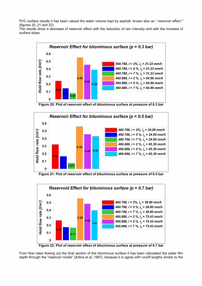
PVC surface results it has been valued the water volume kept by asphalt, known also as " reservoir effect " (figures 20, 21 and 22). The results show a decrease of reservoir effect with the reduction of rain intensity and with the increase of surface slope.

0

0.2

0.4

0.6

0.1

0.3

0.5

Hol

d flo

w ra

te [l

/m2 ]

0.240.14

0.08

0.550.46

0.39

460.788, i = 2%, ip = 21.23 mm/h460.788, i = 5 %, ip = 21.23 mm/h460.788, i = 7 %, ip = 21.23 mm/h460.888, i = 2 %, ip = 64.96 mm/h460.888, i = 5 %, ip = 64.96 mm/h460.888, i = 7 %, ip = 64.96 mm/h

Reservoir Effect for bituminous surface (p = 0.3 bar)

Figure 20: Plot of reservoir effect of bituminous surface at pressure of 0.3 bar

0

0.2

0.4

0.6

0.1

0.3

0.5

Hol

d flo

w r

ate

[l/m

2 ]

0.32

0.160.075

0.560.46 0.43


Reservoir Effect for bituminous surface (p = 0.5 bar)


0

0.2

0.4

0.6

0.1

0.3

0.5

Hol

d flo

w r

ate

[l/m

2 ]

0.260.17 0.17

0.560.48

0.4


Reservoid Effect for bituminous surface (p = 0.7 bar)


From flow rates flowing out the final section of the bituminous surface it has been calculated the water film depth through the “reservoir model” (Artina et al, 1997), because it is agree with runoff lengths similar to the

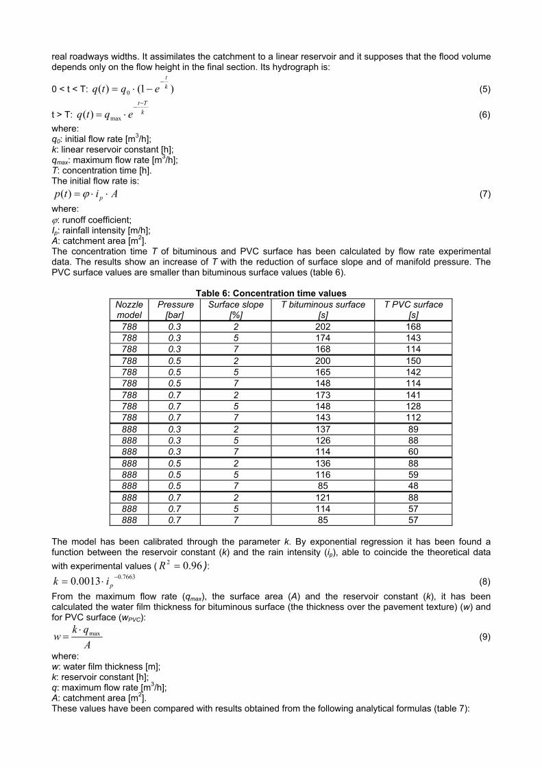
real roadways widths. It assimilates the catchment to a linear reservoir and it supposes that the flood volume depends only on the flow height in the final section. Its hydrograph is:

0 < t < T: )1()( 0kt

eqtq−

−⋅= (5)

t > T: kTt

eqtq−

−⋅= max)( (6)

where: q0: initial flow rate [m3/h]; k: linear reservoir constant [h]; qmax: maximum flow rate [m3/h]; T: concentration time [h]. The initial flow rate is:

Aitp p ⋅⋅= ϕ)( (7) where: ϕ: runoff coefficient; Ip: rainfall intensity [m/h]; A: catchment area [m2]. The concentration time T of bituminous and PVC surface has been calculated by flow rate experimental data. The results show an increase of T with the reduction of surface slope and of manifold pressure. The PVC surface values are smaller than bituminous surface values (table 6).

Table 6: Concentration time values Nozzle model

Pressure [bar]

Surface slope [%]

T bituminous surface [s]

T PVC surface [s]

788 0.3 2 202 168 788 0.3 5 174 143 788 0.3 7 168 114 788 0.5 2 200 150 788 0.5 5 165 142 788 0.5 7 148 114 788 0.7 2 173 141 788 0.7 5 148 128 788 0.7 7 143 112 888 0.3 2 137 89 888 0.3 5 126 88 888 0.3 7 114 60 888 0.5 2 136 88 888 0.5 5 116 59 888 0.5 7 85 48 888 0.7 2 121 88 888 0.7 5 114 57 888 0.7 7 85 57

The model has been calibrated through the parameter k. By exponential regression it has been found a function between the reservoir constant (k) and the rain intensity (ip), able to coincide the theoretical data with experimental values ( 96.02 =R ):

7663.00013.0 −⋅= pik (8) From the maximum flow rate (qmax), the surface area (A) and the reservoir constant (k), it has been calculated the water film thickness for bituminous surface (the thickness over the pavement texture) (w) and for PVC surface (wPVC):

Aqkw max⋅

= (9)

where: w: water film thickness [m]; k: reservoir constant [h]; q: maximum flow rate [m3/h]; A: catchment area [m2]. These values have been compared with results obtained from the following analytical formulas (table 7):

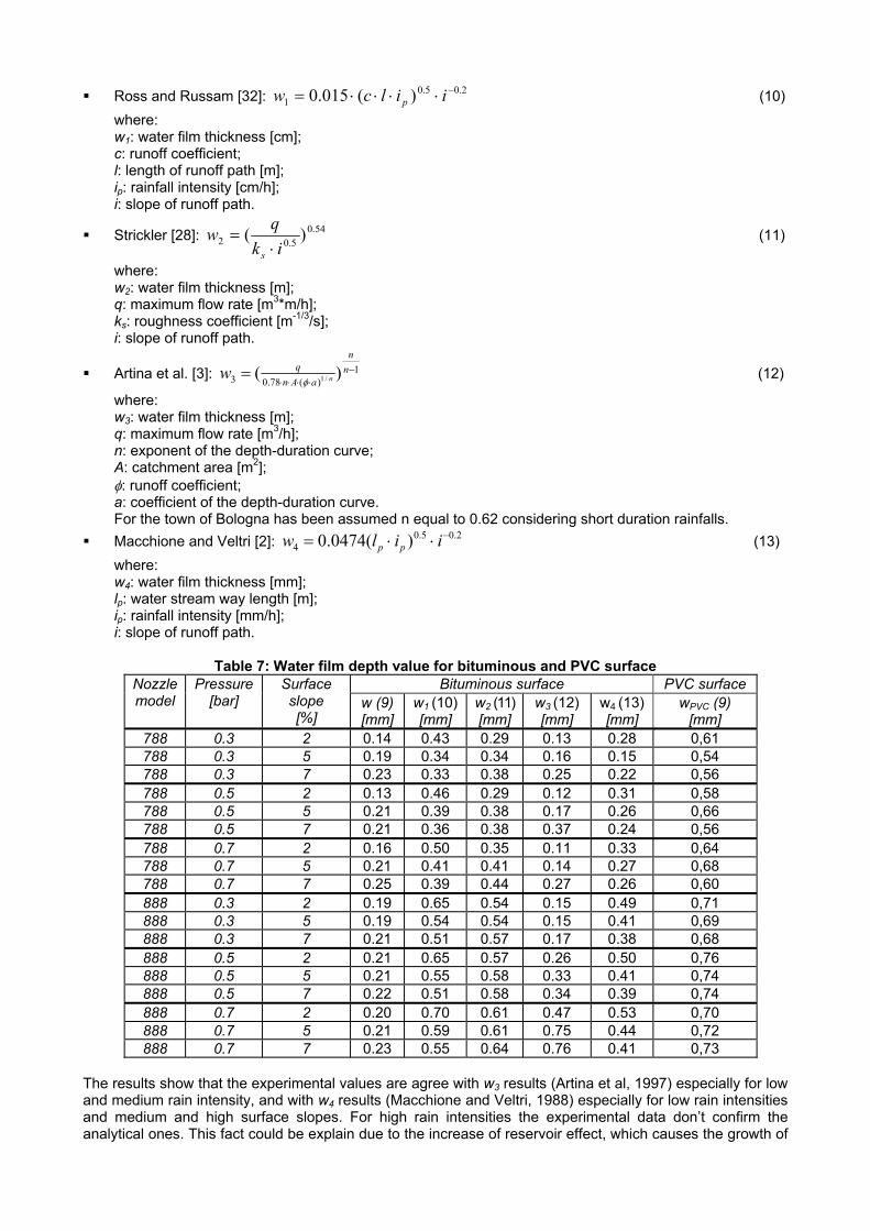
Ross and Russam [32]: 2.05.01 )(015.0 −⋅⋅⋅⋅= iilcw p (10)

where: w1: water film thickness [cm]; c: runoff coefficient; l: length of runoff path [m]; ip: rainfall intensity [cm/h]; i: slope of runoff path.

Strickler [28]: 54.05.02 )(

ikqw

s ⋅= (11)

where: w2: water film thickness [m]; q: maximum flow rate [m3*m/h]; ks: roughness coefficient [m-1/3/s]; i: slope of runoff path.

Artina et al. [3]: 1)(78.03 )( /1

−⋅⋅⋅⋅

= nn

aAnq

nwφ

(12)

where: w3: water film thickness [m]; q: maximum flow rate [m3/h]; n: exponent of the depth-duration curve; A: catchment area [m2]; φ: runoff coefficient; a: coefficient of the depth-duration curve. For the town of Bologna has been assumed n equal to 0.62 considering short duration rainfalls.

Macchione and Veltri [2]: 2.05.04 )(0474.0 −⋅⋅= iilw pp (13)

where: w4: water film thickness [mm]; lp: water stream way length [m]; ip: rainfall intensity [mm/h]; i: slope of runoff path.

Table 7: Water film depth value for bituminous and PVC surface Bituminous surface PVC surface Nozzle

model Pressure

[bar] Surface slope [%]

w (9) [mm]

w1 (10) [mm]

w2 (11)[mm]

w3 (12) [mm]

w4 (13) [mm]

wPVC (9) [mm]

788 0.3 2 0.14 0.43 0.29 0.13 0.28 0,61 788 0.3 5 0.19 0.34 0.34 0.16 0.15 0,54 788 0.3 7 0.23 0.33 0.38 0.25 0.22 0,56 788 0.5 2 0.13 0.46 0.29 0.12 0.31 0,58 788 0.5 5 0.21 0.39 0.38 0.17 0.26 0,66 788 0.5 7 0.21 0.36 0.38 0.37 0.24 0,56 788 0.7 2 0.16 0.50 0.35 0.11 0.33 0,64 788 0.7 5 0.21 0.41 0.41 0.14 0.27 0,68 788 0.7 7 0.25 0.39 0.44 0.27 0.26 0,60 888 0.3 2 0.19 0.65 0.54 0.15 0.49 0,71 888 0.3 5 0.19 0.54 0.54 0.15 0.41 0,69 888 0.3 7 0.21 0.51 0.57 0.17 0.38 0,68 888 0.5 2 0.21 0.65 0.57 0.26 0.50 0,76 888 0.5 5 0.21 0.55 0.58 0.33 0.41 0,74 888 0.5 7 0.22 0.51 0.58 0.34 0.39 0,74 888 0.7 2 0.20 0.70 0.61 0.47 0.53 0,70 888 0.7 5 0.21 0.59 0.61 0.75 0.44 0,72 888 0.7 7 0.23 0.55 0.64 0.76 0.41 0,73

The results show that the experimental values are agree with w3 results (Artina et al, 1997) especially for low and medium rain intensity, and with w4 results (Macchione and Veltri, 1988) especially for low rain intensities and medium and high surface slopes. For high rain intensities the experimental data don’t confirm the analytical ones. This fact could be explain due to the increase of reservoir effect, which causes the growth of

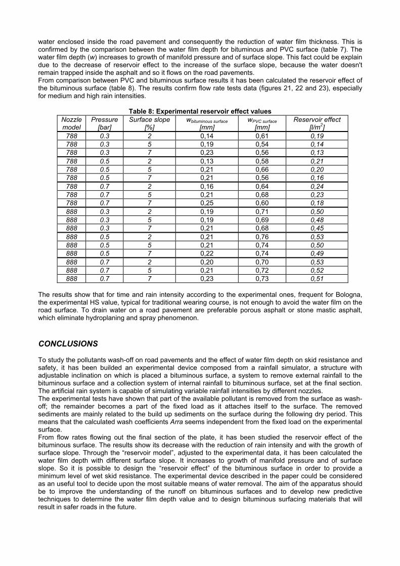
water enclosed inside the road pavement and consequently the reduction of water film thickness. This is confirmed by the comparison between the water film depth for bituminous and PVC surface (table 7). The water film depth (w) increases to growth of manifold pressure and of surface slope. This fact could be explain due to the decrease of reservoir effect to the increase of the surface slope, because the water doesn't remain trapped inside the asphalt and so it flows on the road pavements. From comparison between PVC and bituminous surface results it has been calculated the reservoir effect of the bituminous surface (table 8). The results confirm flow rate tests data (figures 21, 22 and 23), especially for medium and high rain intensities.

Table 8: Experimental reservoir effect values Nozzle model

Pressure [bar]

Surface slope [%]

wbituminous surface [mm]

wPVC surface [mm]

Reservoir effect [l/m2]

788 0.3 2 0,14 0,61 0,19 788 0.3 5 0,19 0,54 0,14 788 0.3 7 0,23 0,56 0,13 788 0.5 2 0,13 0,58 0,21 788 0.5 5 0,21 0,66 0,20 788 0.5 7 0,21 0,56 0,16 788 0.7 2 0,16 0,64 0,24 788 0.7 5 0,21 0,68 0,23 788 0.7 7 0,25 0,60 0,18 888 0.3 2 0,19 0,71 0,50 888 0.3 5 0,19 0,69 0,48 888 0.3 7 0,21 0,68 0,45 888 0.5 2 0,21 0,76 0,53 888 0.5 5 0,21 0,74 0,50 888 0.5 7 0,22 0,74 0,49 888 0.7 2 0,20 0,70 0,53 888 0.7 5 0,21 0,72 0,52 888 0.7 7 0,23 0,73 0,51

The results show that for time and rain intensity according to the experimental ones, frequent for Bologna, the experimental HS value, typical for traditional wearing course, is not enough to avoid the water film on the road surface. To drain water on a road pavement are preferable porous asphalt or stone mastic asphalt, which eliminate hydroplaning and spray phenomenon.

CONCLUSIONS To study the pollutants wash-off on road pavements and the effect of water film depth on skid resistance and safety, it has been builded an experimental device composed from a rainfall simulator, a structure with adjustable inclination on which is placed a bituminous surface, a system to remove external rainfall to the bituminous surface and a collection system of internal rainfall to bituminous surface, set at the final section. The artificial rain system is capable of simulating variable rainfall intensities by different nozzles. The experimental tests have shown that part of the available pollutant is removed from the surface as wash-off; the remainder becomes a part of the fixed load as it attaches itself to the surface. The removed sediments are mainly related to the build up sediments on the surface during the following dry period. This means that the calculated wash coefficients Arra seems independent from the fixed load on the experimental surface. From flow rates flowing out the final section of the plate, it has been studied the reservoir effect of the bituminous surface. The results show its decrease with the reduction of rain intensity and with the growth of surface slope. Through the “reservoir model”, adjusted to the experimental data, it has been calculated the water film depth with different surface slope. It increases to growth of manifold pressure and of surface slope. So it is possible to design the “reservoir effect” of the bituminous surface in order to provide a minimum level of wet skid resistance. The experimental device described in the paper could be considered as an useful tool to decide upon the most suitable means of water removal. The aim of the apparatus should be to improve the understanding of the runoff on bituminous surfaces and to develop new predictive techniques to determine the water film depth value and to design bituminous surfacing materials that will result in safer roads in the future.

REFERENCES 1. Alley, W.M. (1981), Estimation of impervious-area wash-off parameters, Water resources Research, vol.

17, n. 4, pp. 1161-1166. 2. Ammon D.C. (1979), Urban stormwater pollutant buildup and wash-off relationship, Master of

Engineering Thesis, University of Florida, Dept. of Environmental Engineering Sciences, Gainesville, Florida;

3. Artina, S., Modica, C., Paoletti, A., Maglionico, M. & Marinelli A. (1997), Modelli matematici di drenaggio urbano, Sistemi di Fognatura. Manuale di Progettazione, Sottogruppo Deflussi Urbani del Gruppo Nazionale di Idraulica, Ed. Hoepli.

4. Becchi, I., Caporali, E., Castelli, F. & Lorenzini, C. (2001), Field study of water film produced by intense rainfall on a road pavements, Proc. of II International Colloquium on Vehicle-Tyre-Road Interaction, Firenze, Italia, pp. 113-132.

5. Bocci, M. & Cerni, G. (1997), Influenza delle polveri sull’attrito radente nelle pavimentazioni stradali, Workshop “La sicurezza intrinseca delle infrastrutture stradali”, Roma, Italia, pp. 351-362.

6. Caporali, E., Castelli, F. & Lorenzini, C. (2000), La dinamica dei veli idrici sulla pavimentazione stradale: indagini sul campo, Proc. of XXVII National Congress of Hydraulics and Hydraulic Construction, Genova, Italia, pp. 19-26.

7. Cera, L. & Di Mascio, P. (1998), Modello previsionale dell’inquinamento prodotto dalle acque di ruscellamento stradale: analisi nei corpi idrici ricettori, Proc. of. XXIII Convegno Nazionale Stradale, Verona, Italia, pp. 45-52.

8. Cera, L. & Di Mascio, P. (2001), Trattamento e riciclaggio delle acque di ruscellamento stradale, Proc. of XI Convegno Nazionale SIIV, Verona, Italia, pp. 1-15.

9. CNR (1983), Norme per la misura delle caratteristiche superficiali delle pavimentazioni: Metodo di prova per la misura della macro-rugosità superficiale con il sistema della altezza in sabbia, B.U. n° 94.

10. CNR (1985), Norme per la misura delle caratteristiche superficiali delle pavimentazioni: Metodo di prova per la misura della resistenza di attrito radente con l’apparecchio portatile a pendolo, B.U. n° 105.

11. Di Mascio, P. (1994), Incidentalità e caratteristiche superficiali delle pavimentazioni stradali, Proc. of XXII Convegno Nazionale Stradale AIPCR, Perugia, Italia.

12. Domenichini, L. & Cera, L. (1994), Distribuzione areale dei veli idrici su piani stradali, Proc. of XXII Convegno Nazionale Stradale AIPCR, Perugia, Italia, pp. 135-140.

13. Domenichini, L. & La Torre, F. (1995), Relationship between friction, surface, characteristics and rain intensities to evacuate roadway safety, International Forum on Road Safety Research, Bangkok, Thailand.

14. Domenichini, L. & La Torre, F. (1997), Valutazione della sicurezza attraverso l’analisi del rapporto tra aderenza, caratteristiche superficiali ed intensità di pioggia, Workshop “La sicurezza intrinseca delle infrastrutture stradali”, Roma, Italia, pp. 585-597.

15. Domenichini, L. & Remedia, G. (1992), Condizioni di deflusso su piani stradali in zone di transizione, Proc. of XXIII National Congress of Hydraulics and Hydraulic Construction, Firenze, Italia, pp. 127-133.

16. Domenichini, L. & Remedia G. (1994), Il rischio di aquaplaning in zone di transizione stradali, Proc. of XXII Convegno Nazionale Stradale AIPCR, Perugia, Italia, pp. 23-34.

17. French, T., Tyre Technology, Ed. Adam Hilger. 18. Ford, T.L. & Charles F.S. (1988), Heavy Duty Truck Tire Engineering, SAE Paper no. 880001. 19. Giannini, F. & Noli, A. (1974), Il deflusso dell’acqua sulle superfici stradali, Autostrade, n. 4, pp. 9-25. 20. Göhring, E., Von Glasner, E.C. & Pflug, H.C. (1991), Contribution to the Force Transmission Behaviour

of Commercial Vehicle Tires, SAE Paper no. 912692. 21. Gothié, M., Parry, T. & Roe, P. (2001), The relative influence of the parameters affecting road surface

friction, Proc. of II International Colloquium on Vehicle-Tyre-Road Interaction, Firenze, Italia. 22. Gunn, R. & Kinzer, G.D. (1949), Terminal velocity of water droplets in stagnant air, Journal of

meteorology, vol. 6. 23. Jewell, T.K. & Adrian, D.D. (1982), Statistical analysis to drive improved stormwater quality-models,

Journal of Water Pollution Control Federation, vol. 54, n.5. 24. Laws, J.O. (1941), Measurements of fall-velocity of water-droops and rain-drops, Transaction of the

American Geophysics Union, vol. 24. 25. Laws, J.O. & Parsons, D.A. (1943), The relation of drop size to intensity, Transactions of the American

Geophysical Union, vol. 26, pp. 456-460. 26. Lorenzini, C. & Becchi, I. (2000), Un apparato sperimentale per lo studio dei veli idrici di origine

meteorica su superfici impermeabili, Proc. of XXVII National Congress of Hydraulics and Hydraulic Construction, Genova, Italia, pp. 105-109.

27. Panini, T., Salvador Sanchis, M.P. & Torri, D. (1993), A portable rainfall simulator for rough and smooth morphologies, Quaderni di scienza del suolo, vol. 45, pp. 47-58.

28. Pasetto, M. & Zanutto, G. (2001), Studio del deflusso delle acque meteoriche nelle curve di transizione dei tracciati stradali: applicazione a livellette brevi con ciglio ad andamento altimetrico variabile nello spazio, Workshop “La sicurezza intrinseca delle infrastrutture stradali”, Roma, Italia, pp. 303-331.

29. Pauwelussen, J.P. (2002), Adherence under special road conditions, European Tyre School, module n. 10.

30. Raaberg, J. (2000), Examination of pollution in soil and water along roads caused by traffic and road pavement, Danish Road Institute, report 104.

31. Romkens M. J. M., Helming K. & Prasad S. N. (2001), Soil erosion under different rainfall intensities, surface roughness and soil water regimes, Catena, vol. 46, pp. 130-123.

32. Ross, N. F. & Russam, K. (1968), The depth of rain water on road surface, Road Research Laboratory, Ministry of Transport, RRL Report LR 236.

33. Sartor, J.D. & Boyd, G.B. (1972), Water Pollution Aspects of Street Surface Contaminants, United States Environmental Protection Agency, Washington, DC, EPA-R2-72-081.

34. Sartor, J.D., Boyd, G.B. & Agardy, F.J. (1974), Water pollution aspects of street surface contamination, Journal of Water Pollution Control Federation, vol. 46, n.3.

35. Sonne M. B. (1980), Urban runoff quality: information needs, ASCE, vol. 106, pp. 29-40. 36. Tomanovic, A. & Maksimovic, C. (1996), Improved modelling of suspended solids discharge from

asphalt surface during storm event, Water Science and Technology, vol. 33, n. 4, pp. 363-369. 37. Vaze, J. & Chiew, F.H.S. (2002), Experimental study of pollutant accumulation on an urban road

surface, Urban Water, vol. 4, pp. 379-389.

ACKNOWLEDGEMENTS We take this opportunity to thank Eng. Barbara Falò and Eng. Francesco Grandi for the considerable help they gave us in carrying out the tests. The authors gratefully acknowledge also the support of Mr. Lunardi of Sintexcal S.p.a.

Documents

Surface Runoff: A Rainfall Simulator For Wash-Off …...Surface Runoff: A Rainfall Simulator For Wash-Off Modelling And Road Safety Auditing Under Different Rainfall Intensities Simone