Embed Size (px)
Citation preview

l
TechnicaSurfacing
StudioTools 12Copyright and trademarks
StudioTools 13
Software copyright information is located in the application, and can be accessed from the menu by choosing Help > About StudioTools.
All documentation ("Documentation") is copyrighted © 2001-2005 Alias and contains proprietary and confidential information of Alias. The Documentation is protected by national and international intellectual property laws and treaties. All rights reserved. Use of the Documentation is subject to the terms of the license agreement that governs the use of the software product to which the Documentation pertains ("Software"). The authorized licensee of the Software is hereby authorized to print no more than one (1) hardcopy of any Documentation provided in digital format per valid license of the Software held by such licensee. Except for the foregoing, the Documentation may not be translated, copied or duplicated in any form (physically or electronically), in whole or in part, without the prior written consent of Alias.
Alias and the swirl logo, Maya and DesignStudio are registered trademarks and Alias Natural Phenomena, Alias OpenAlias, Alias OpenModel, Alias PowerCaster, Alias PowerTracer, Alias RayCasting, Alias RayTracing, Alias SDL, ImageStudio, Alias Spider, StudioPaint, StudioViewer, StudioTools and SurfaceStudio are trademarks of Alias Systems Corp. ("Alias") in the United States and/or other countries. Silicon Graphics, SGI and IRIX are registered trademarks and Inventor is a trademark of Silicon Graphic, Inc. in the United States and/or other countries worldwide. Microsoft and Windows are either registered trademarks or trademarks of Microsoft Corporation in the United States and/or other countries. Renderman is a registered trademark of Pixar Corporation. Apple, Quicktime and Macintosh are trademarks of Apple Computer, Inc. registered in the United States and other countries. Adobe, Postcript and Illustrator are either registered trademarks or trademarks of Adobe Systems Incorporated in the United States and/or other countries. Unigraphics, NX, and I-deas are registered trademarks or trademarks of UGS Corp. or its subsidiaries in the United States and in other countries. Arius3D is a registered trademark of Arius3D Inc. Cyberware is a registered trademark of Cyberware Laboratory Inc.. Cyrax is a registered trademark of Leica Geosystems HDS Inc. Steinbichler is a registered trademark of Steinbichler Optotechnik GmbH. Autodesk and AutoCAD are either registered trademarks or trademarks of Autodesk, Inc./Autodesk Canada, Inc. in the USA and/or other countries. CATIA is a registered trademark of Dassault Systèmes S.A. PTC, Pro/ENGINEER and Granite are trademarks or registered trademarks of Parametric Technology Corporation or its subsidiaries in the U.S. and in other countries. All other trademarks mentioned herein are the property of their respective owners.
All PTC Technology logos are used under license from Parametric Technology Corporation, Needham, MA, USA.
Not all features described are available in all products.
Alias Systems Corp., 210 King Street East, Toronto, Canada M5A 1J7

CONTENTS
Contents vLearning Technical Surfacing vii
Introduction to Tech-nical Surfacing Tutori-als vii
Interface Basics 1Introduction 1Installing the tutorial courseware files 1Starting StudioTools 2Overview of the Stu-dioTools Interface 4Using Help 5Arranging Windows 5Tool Basics 9Using a Snap Mode 10Picking and Unpicking Objects 13Shortcuts to Tools 16Creating Custom Shelves 16
Using and Customizing Marking Menus 21Using hot keys 23Tracking, Dollying, and Tumbling the Camera’s View 25Changing the Point of Interest 28Using the Viewing Panel 29Types of Nodes 34The SBD window 35Conclusion 36
Introduction to the Tutorial 37Some Common Modeling Basics 39
Quality Defines the Model 39How Different Types of Input Affect the Model 40Loading and Organizing Data 41Interface Arrangement 43Traditional Surface Modeling 45
Creating and Fitting Curves 49Creating blends between the main curves 52An explanation of Continuity types 53Fitting Curves to X-scans 58Fitting Curves to Z-scans 62
Surface Creation 67Introduction to Patch Layouts 67The Importance of Helper Surfaces 68Understanding and Refining the Theoretical Model 69
Constructing the Main Surfaces 77Extending the Theoretical Line 77Constructing the Side Surface 78Constructing the Top Surface 82Applying a Transition Between the Front and Top Surfaces 88Applying a Transition Between the Rear and Top Surfaces 95
Transition Surfaces 101Constructing Simple Transitions 101Constructing a Transition Surface at the Rear of the Model 107Constructing Ball Corners 110
Finishing the Model 119Advanced Surface Modeling 121
Handling Blend Curves 122Crucial Blend Curve Tools 123Information Provided by Blend Curves 124Blend Curves as Transition Curves 128Software versions below SurfaceStudio 10.1 128Blend Curve Constraint to a Surface Edge 130Blend Curve Constraint to an ISO parameter 131
v

Blend Curve Constraint to a Curve-On-Surface 131Blend Curve Constraint to a Curve 132Understanding the Align Tool 133Handling the Align Tool 133Basics of surface fillets 141Selection Process 141Undo All 145Addressing Interior Breaks in Continuity 146When to use Bezier Surfaces instead of NURBS Geometry 146When to use NURBS Geometry instead of Bezier Geometry 148Choosing the Right Curve for the Job 149Surface Continuity 151Model Check 152Dynamic Section 154Clipping Plane 154Minimum Radii 155CV Distribution 156Span Distribution 157Surface Evaluation 158
viContents

LEARNING TECHNICAL SURFACING
Learning objectives
● Background information about SurfaceStudio and the tutorials
● Determining your learning level
● Conventions used in these tutorials
Introduction to Technical Surfacing Tutorials
A general overview of the tutorials.
Alias StudioTools provides a complete set of interactive surfacing, modification, and evaluation tools for creating surface models that meet the demanding levels of quality and precision required in manufacturing.
In this book, we will present examples of typical production workflows using StudioTools. We will introduce powerful tools and interactive features available in SurfaceStudio and AutoStudio, and demonstrate how to use them to accomplish your surfacing tasks.
These tutorials are densely packed with information and techniques that may be new to you. You may want to re-read the lessons after completion, or even repeat the more difficult lessons.
Some techniques, especially those related to fitting curves and direct modeling, are interactive and can be challenging. You may want to practice these skills after completing the tutorials.
For more information
Note that these tutorials are introductions to technical surfacing solutions and workflows. They are not intended as an exhaustive guide to the capabilities and options of the StudioTools tools. These tutorials are designed to work with SurfaceStudio, but will also work with AutoStudio and Studio with Advanced
For additional information and more comprehensive explanations of tools and options, refer to the Modeling in StudioTools section of the online documentation.
1
Where to begin
Establish what learning level you are at before starting.
The first tutorial covers some material that may already be familiar to you. You can make decisions about these tutorials based on whether you are an absolute beginner, already familiar with Silicon Graphics workstations, or already familiar with Alias Systems StudioTools products.
> Absolute Beginners
You should start the tutorials at the very beginning of Lesson : Interface Basics on page 5, work through all of the Modeling tutorials, and then move on to the Foundations of Surface Modeling tutorial.
> Users Familiar With Silicon Graphics Workstations
You should log into your account (or the common StudioTools account) on your workstation and then start the tutorials with the instructions for Starting StudioTools (page 6).
> Users Familiar With Alias Systems Studio Products
Much of the first chapter deals with interface basics common to all Studio products. However, you will still want to familiarize yourself with new or SurfaceStudio-specific features.
Graphic Conventions
Explains graphic conventions used in the tutorials
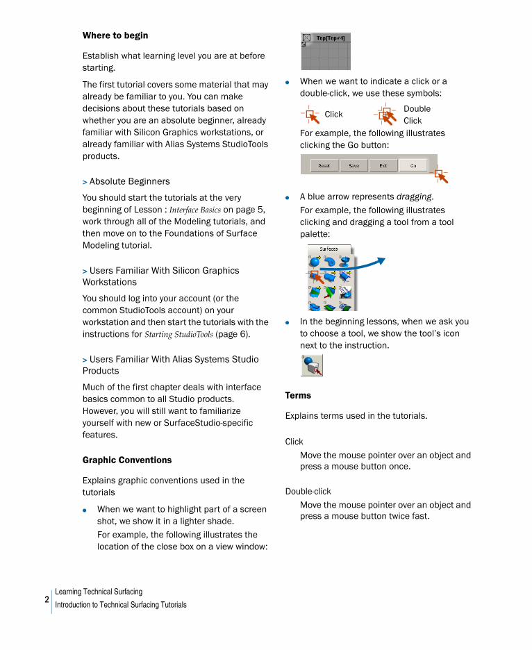
● When we want to highlight part of a screen shot, we show it in a lighter shade.
For example, the following illustrates the location of the close box on a view window:
● When we want to indicate a click or a double-click, we use these symbols:
For example, the following illustrates clicking the Go button:
● A blue arrow represents dragging.
For example, the following illustrates clicking and dragging a tool from a tool palette:
● In the beginning lessons, when we ask you to choose a tool, we show the tool’s icon next to the instruction.
Terms
Explains terms used in the tutorials.
Click
Move the mouse pointer over an object and press a mouse button once.
Double-click
Move the mouse pointer over an object and press a mouse button twice fast.
ClickDouble Click
2Learning Technical Surfacing
Introduction to Technical Surfacing Tutorials

Drag
Move the mouse pointer over an object and hold down a mouse button. Then move the mouse with the button held down.
The Scene
The 3D “world” inside the view windows.
The Model
The curves, surfaces, and points that make up the object you are creating.
3Learning Technical Surfacing
Introduction to Technical Surfacing Tutorials

4Learning Technical Surfacing
Introduction to Technical Surfacing Tutorials
INTERFACE BASICS
Learning objectives
You will learn how to:
● Log into the system and start StudioTools.
● Arrange windows.
● Use tools and tool options.
● Customize shelves and marking menus.
● Tumble, track, and dolly the view.
● Use the Object Lister window to understand the model
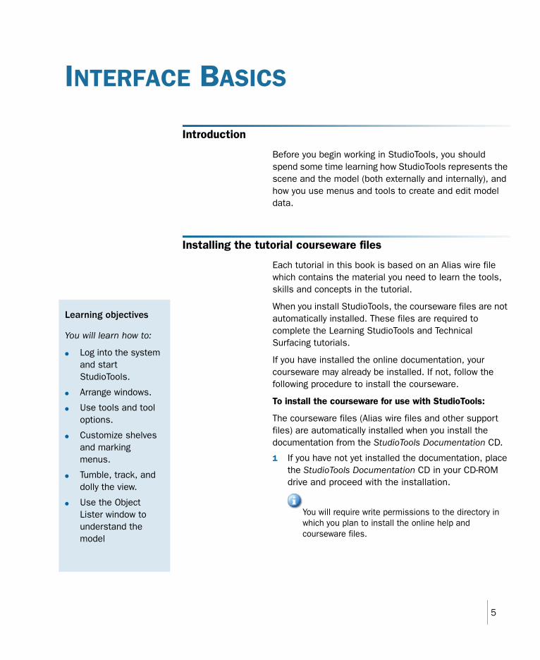
Introduction
Before you begin working in StudioTools, you should spend some time learning how StudioTools represents the scene and the model (both externally and internally), and how you use menus and tools to create and edit model data.
Installing the tutorial courseware files
Each tutorial in this book is based on an Alias wire file which contains the material you need to learn the tools, skills and concepts in the tutorial.
When you install StudioTools, the courseware files are not automatically installed. These files are required to complete the Learning StudioTools and Technical Surfacing tutorials.
If you have installed the online documentation, your courseware may already be installed. If not, follow the following procedure to install the courseware.
To install the courseware for use with StudioTools:
The courseware files (Alias wire files and other support files) are automatically installed when you install the documentation from the StudioTools Documentation CD.
1 If you have not yet installed the documentation, place the StudioTools Documentation CD in your CD-ROM drive and proceed with the installation.
You will require write permissions to the directory in which you plan to install the online help and courseware files.
5

If you want to install only the courseware files, go directly to your disk drive and find the CourseWare folder on the disk.
2 Copy the CourseWare folder from its location on your hard drive or CD-ROM drive into your user_data folder.On Windows systems this is typically:C:\Documents and Settings\[userid]\My Documents\StudioTools\user_data\CourseWare
On UNIX systems this is typically:$HOME/user_data/CourseWare
To install the courseware for use with StudioTools Personal Learning Edition
1 The StudioTools documentation should have already been installed on your system. The courseware files you’ll require
to perform the tutorials can be found in the CourseWare directory, located under the Help directory. If the documentation has not been installed on your computer, insert the Documentation CD and install it. You will require write permissions to the directory in which you plan to install the online help and courseware files.
2 Copy the CourseWare directory from the Help directory to your account’s user data directory.On Windows systems this is typically:C:\Documents and Settings\[userid]\My Documents\StudioTools\user_data\CourseWare
On UNIX systems this is typically:$HOME/user_data/CourseWare
Starting StudioTools
Logging In
If you have not logged in to your account on your workstation, do so now.
To log in to your account
● Type your user name and password at the prompts.If you have an account on this workstation, the operating system user environment will appear.
Depending on which product you are using, the StudioTools icon may have a different name, such as DesignStudio or AutoStudio.
To start StudioTools on Windows
1 Double-click the Studio shortcut icon on the desktop, or choose Studio from the Start menu. When you start StudioTools for the first time the Application Launcher appears on your desktop.
2 Choose a product to launch and options where applicable. If you want StudioTools to launch the selected product and options automatically every time you start StudioTools, click Set Default. When you start StudioTools again, the default product starts and the Application Launcher does not appear. You can change the default settings anytime by choosing Application Launcher from the Start menu.
3 Click Launch. The chosen product should start.
6Starting StudioTools

4 If the main StudioTools window appears, StudioTools is installed.
To start StudioTools on UNIX
1 Go to the Toolchest menu on your desktop. Choose Find > Icon Catalog.The Icon Catalog opens.
2 Go to the Alias Systems software page.
3 Double-click the StudioTools icon. When you start StudioTools for the first time the Application Launcher appears on your desktop.
4 Choose a product to launch and options where applicable. If you want StudioTools to launch the selected product and options automatically every time you start StudioTools, click Set Default. When you start StudioTools again, the default product starts and the Application Launcher does not appear. You can change the default settings anytime by choosing Application Launcher from the Start menu.
5 Click Launch. The chosen product should start.
6 If the main StudioTools window appears, StudioTools is installed.
7Starting StudioTools
The Start-up Process
StudioTools shows the following splash window as it loads:
During start-up, StudioTools may warn you about unusual conditions on your system:
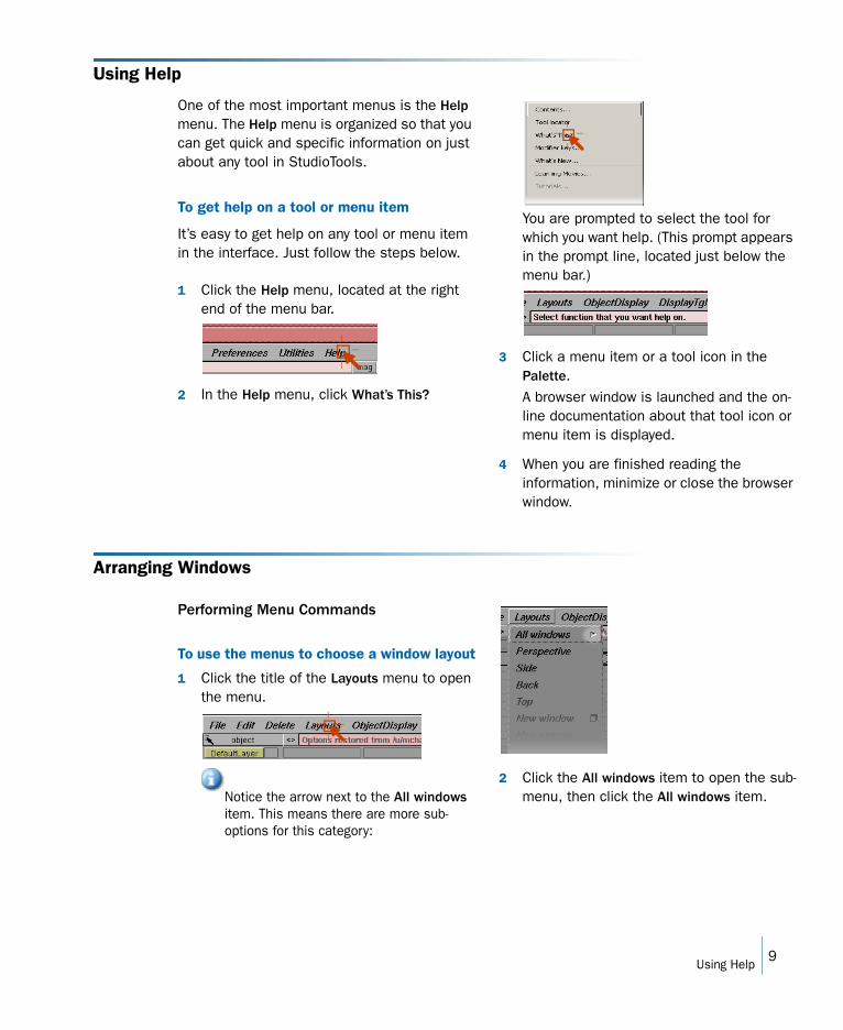
● If you are already running StudioTools (or if StudioTools exited abnormally the last time you ran it), the application will ask you if you really want to start another copy.
If you are sure StudioTools is not running, click Yes to continue loading.
Once StudioTools has finished loading its resources and plug-ins, the workspace window opens.
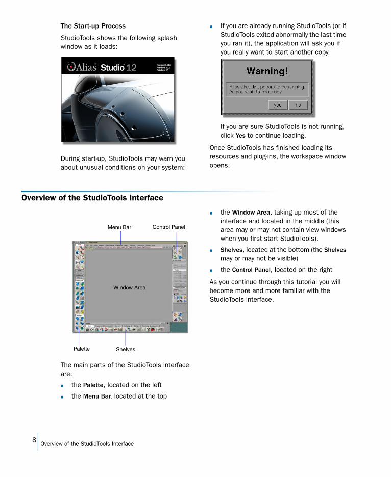
Overview of the StudioTools Interface
The main parts of the StudioTools interface are:
● the Palette, located on the left
● the Menu Bar, located at the top
● the Window Area, taking up most of the interface and located in the middle (this area may or may not contain view windows when you first start StudioTools).
● Shelves, located at the bottom (the Shelves may or may not be visible)
● the Control Panel, located on the right
As you continue through this tutorial you will become more and more familiar with the StudioTools interface.
Menu Bar
Shelves
Control Panel
Window Area
Palette
8Overview of the StudioTools Interface
Using Help
One of the most important menus is the Help menu. The Help menu is organized so that you can get quick and specific information on just about any tool in StudioTools.
To get help on a tool or menu item
It’s easy to get help on any tool or menu item in the interface. Just follow the steps below.
1 Click the Help menu, located at the right end of the menu bar.
2 In the Help menu, click What’s This?
You are prompted to select the tool for which you want help. (This prompt appears in the prompt line, located just below the menu bar.)
3 Click a menu item or a tool icon in the Palette. A browser window is launched and the on-line documentation about that tool icon or menu item is displayed.
4 When you are finished reading the information, minimize or close the browser window.
Arranging Windows
Performing Menu Commands
To use the menus to choose a window layout
1 Click the title of the Layouts menu to open the menu.
Notice the arrow next to the All windows item. This means there are more sub-options for this category:
2 Click the All windows item to open the sub-menu, then click the All windows item.
9Using Help
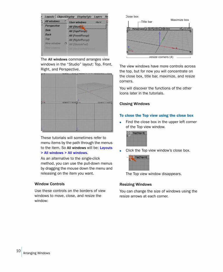
The All windows command arranges view windows in the “Studio” layout: Top, Front, Right, and Perspective.
These tutorials will sometimes refer to menu items by the path through the menus to the item. So All windows will be: Layouts > All windows > All windows.As an alternative to the single-click method, you can use the pull-down menus by dragging the mouse down the menu and releasing on the item you want.
Window Controls
Use these controls on the borders of view windows to move, close, and resize the window:
The view windows have more controls across the top, but for now you will concentrate on the close box, title bar, maximize, and resize corners.
You will discover the functions of the other icons later in the tutorials.
Closing Windows
To close the Top view using the close box
● Find the close box in the upper left corner of the Top view window.
● Click the Top view window’s close box.
The Top view window disappears.
Resizing Windows
You can change the size of windows using the resize arrows at each corner.
Close box
Title barMaximize box
resize corners (4)
10Arranging Windows
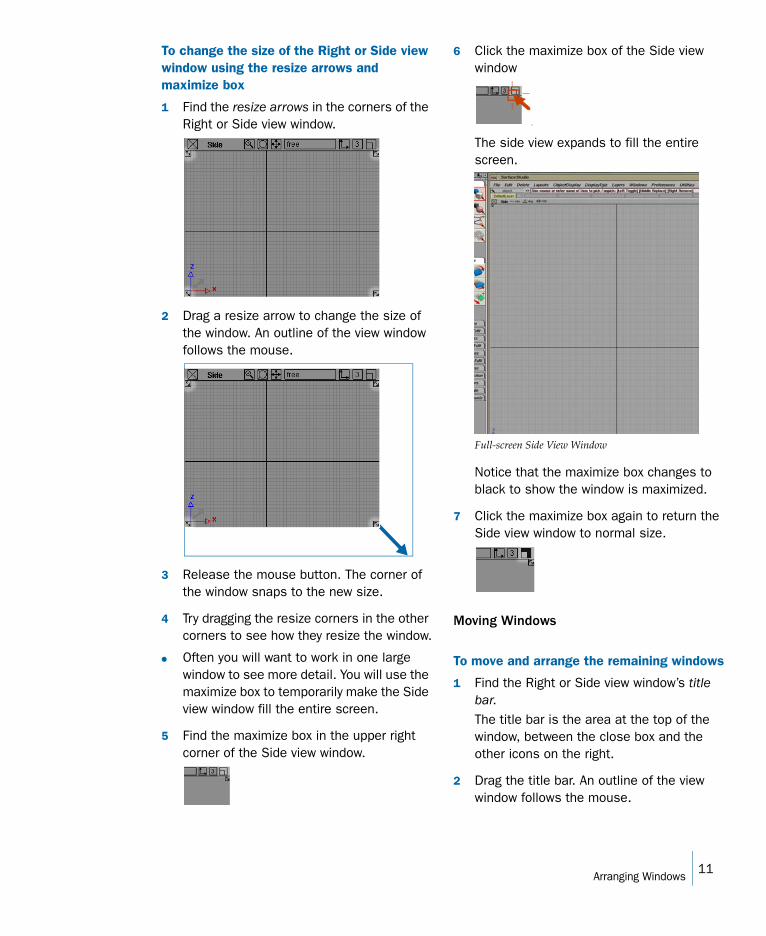
To change the size of the Right or Side view window using the resize arrows and maximize box
1 Find the resize arrows in the corners of the Right or Side view window.
2 Drag a resize arrow to change the size of the window. An outline of the view window follows the mouse.
3 Release the mouse button. The corner of the window snaps to the new size.
4 Try dragging the resize corners in the other corners to see how they resize the window.
● Often you will want to work in one large window to see more detail. You will use the maximize box to temporarily make the Side view window fill the entire screen.
5 Find the maximize box in the upper right corner of the Side view window.
6 Click the maximize box of the Side view window
.
The side view expands to fill the entire screen.
Full-screen Side View Window
Notice that the maximize box changes to black to show the window is maximized.
7 Click the maximize box again to return the Side view window to normal size.
Moving Windows
To move and arrange the remaining windows
1 Find the Right or Side view window’s title bar.The title bar is the area at the top of the window, between the close box and the other icons on the right.
2 Drag the title bar. An outline of the view window follows the mouse.
11Arranging Windows
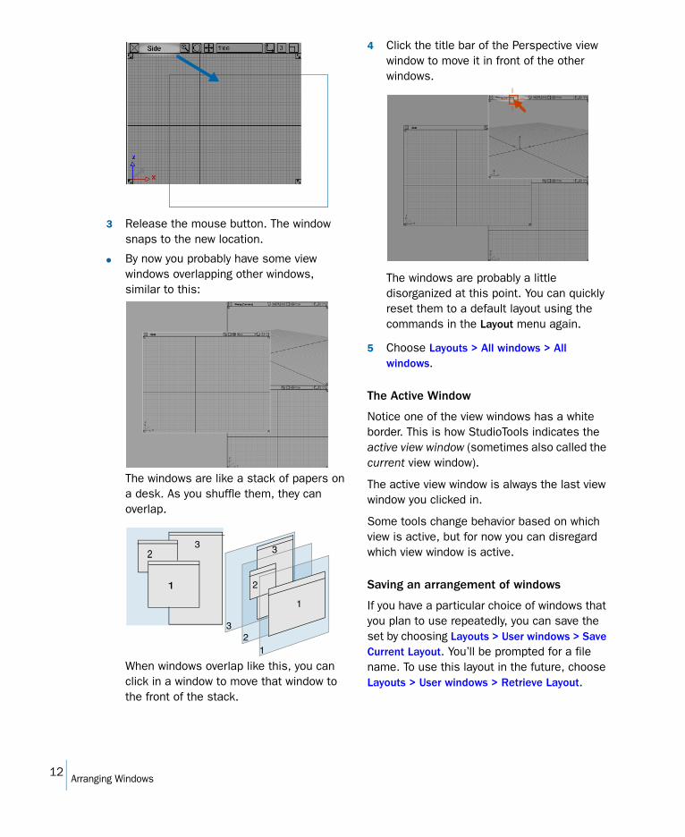
3 Release the mouse button. The window snaps to the new location.
● By now you probably have some view windows overlapping other windows, similar to this:
The windows are like a stack of papers on a desk. As you shuffle them, they can overlap.
When windows overlap like this, you can click in a window to move that window to the front of the stack.
4 Click the title bar of the Perspective view window to move it in front of the other windows.
The windows are probably a little disorganized at this point. You can quickly reset them to a default layout using the commands in the Layout menu again.
5 Choose Layouts > All windows > All windows.
The Active Window
Notice one of the view windows has a white border. This is how StudioTools indicates the active view window (sometimes also called the current view window).
The active view window is always the last view window you clicked in.
Some tools change behavior based on which view is active, but for now you can disregard which view window is active.
Saving an arrangement of windows
If you have a particular choice of windows that you plan to use repeatedly, you can save the set by choosing Layouts > User windows > Save Current Layout. You’ll be prompted for a file name. To use this layout in the future, choose Layouts > User windows > Retrieve Layout.
3
1
2
1
2
3
12
3
12Arranging Windows
Using Tools
Describes how to use the StudioTools interface, such as selecting tools and creating shortcuts.
Tool Basics
To orient yourself in the Palette window
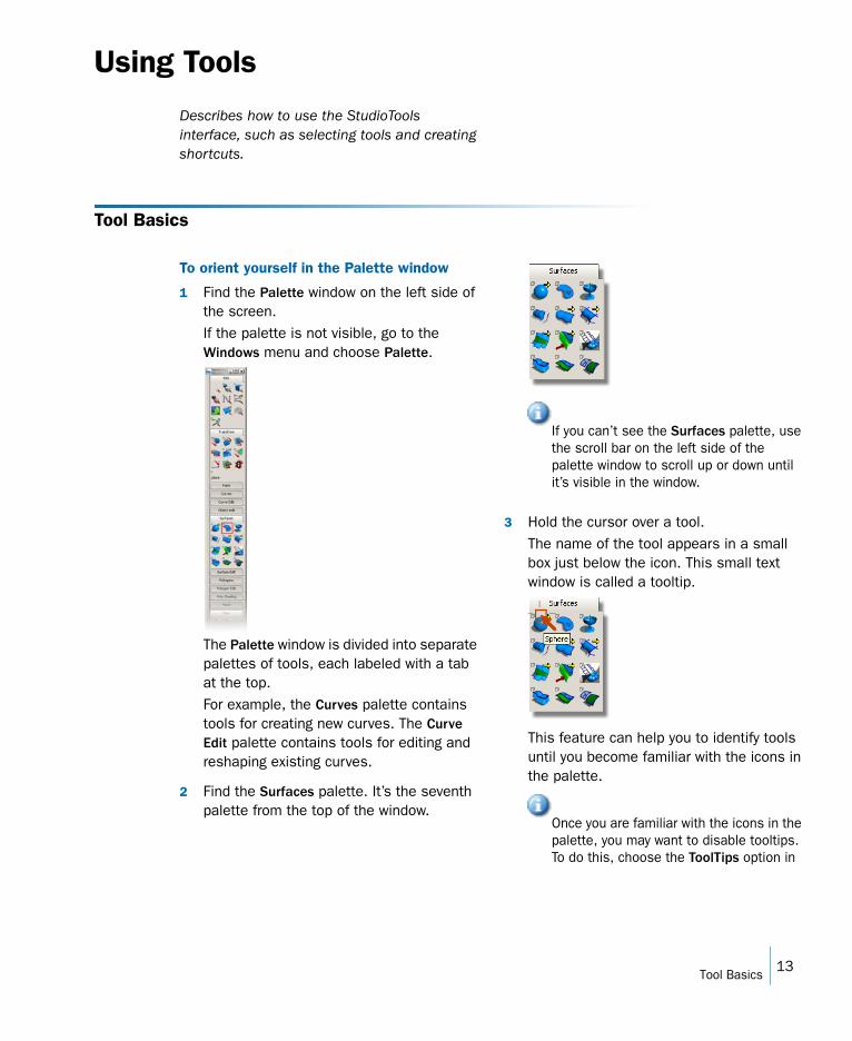
1 Find the Palette window on the left side of the screen.If the palette is not visible, go to the Windows menu and choose Palette.
The Palette window is divided into separate palettes of tools, each labeled with a tab at the top.For example, the Curves palette contains tools for creating new curves. The Curve Edit palette contains tools for editing and reshaping existing curves.
2 Find the Surfaces palette. It’s the seventh palette from the top of the window.
If you can’t see the Surfaces palette, use the scroll bar on the left side of the palette window to scroll up or down until it’s visible in the window.
3 Hold the cursor over a tool. The name of the tool appears in a small box just below the icon. This small text window is called a tooltip.
This feature can help you to identify tools until you become familiar with the icons in the palette.
Once you are familiar with the icons in the palette, you may want to disable tooltips. To do this, choose the ToolTips option in
13Tool Basics
the Interface section of the General Preferences window (Preferences > General Preferences❏).
Now you will use the geometric primitive tools to add some geometry to the scene. The primitive tools create simple 3D geometric shapes such as cubes, spheres, and cones.
As a technical surfacer, you may not regularly need to add these simple shapes to a model. However, they will allow us to practice several StudioTools interface concepts, including choosing tools, using manipulators, sub-palettes, tool option windows, and snapping.
To create a primitive sphere in the scene
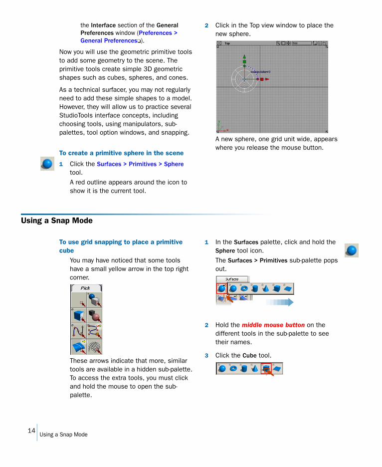
1 Click the Surfaces > Primitives > Sphere tool.A red outline appears around the icon to show it is the current tool.
2 Click in the Top view window to place the new sphere.
A new sphere, one grid unit wide, appears where you release the mouse button.
Using a Snap Mode
To use grid snapping to place a primitive cube
You may have noticed that some tools have a small yellow arrow in the top right corner.
These arrows indicate that more, similar tools are available in a hidden sub-palette. To access the extra tools, you must click and hold the mouse to open the sub-palette.
1 In the Surfaces palette, click and hold the Sphere tool icon.The Surfaces > Primitives sub-palette pops out.
2 Hold the middle mouse button on the different tools in the sub-palette to see their names.
3 Click the Cube tool.
14Using a Snap Mode
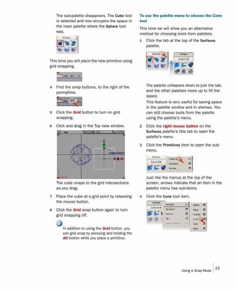
The sub-palette disappears. The Cube tool is selected and now occupies the space in the main palette where the Sphere tool was.
This time you will place the new primitive using grid snapping.
4 Find the snap buttons, to the right of the promptline.
5 Click the Grid button to turn on grid snapping.
6 Click and drag in the Top view window.
The cube snaps to the grid intersections as you drag.
7 Place the cube at a grid point by releasing the mouse button.
8 Click the Grid snap button again to turn grid snapping off.
In addition to using the Grid button, you can grid snap by pressing and holding the Alt button while you place a primitive.
To use the palette menu to choose the Cone tool
This time we will show you an alternative method for choosing tools from palettes.
1 Click the tab at the top of the Surfaces palette.
The palette collapses down to just the tab, and the other palettes move up to fill the space.This feature is very useful for saving space in the palette window and in shelves. You can still choose tools from the palette using the palette’s menu.
2 Click the right mouse button on the Surfaces palette’s title tab to open the palette’s menu.
3 Click the Primitives item to open the sub-menu.
Just like the menus at the top of the screen, arrows indicate that an item in the palette menu has sub-items.
4 Click the Cone tool item.
15Using a Snap Mode
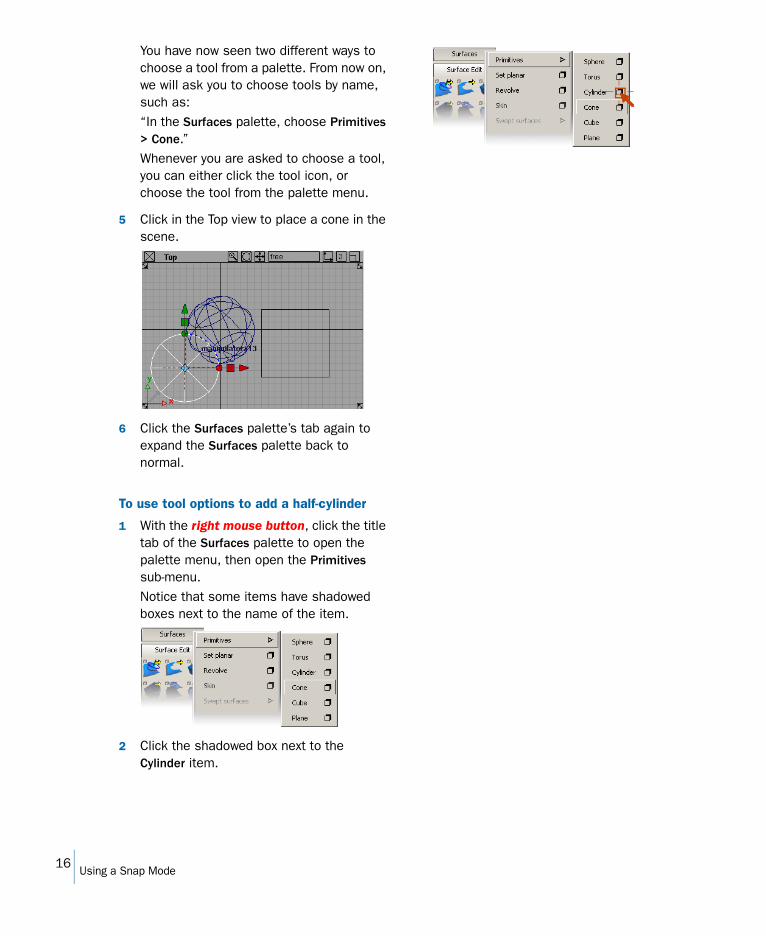
You have now seen two different ways to choose a tool from a palette. From now on, we will ask you to choose tools by name, such as:“In the Surfaces palette, choose Primitives > Cone.”Whenever you are asked to choose a tool, you can either click the tool icon, or choose the tool from the palette menu.
5 Click in the Top view to place a cone in the scene.
6 Click the Surfaces palette’s tab again to expand the Surfaces palette back to normal.
To use tool options to add a half-cylinder
1 With the right mouse button, click the title tab of the Surfaces palette to open the palette menu, then open the Primitives sub-menu.Notice that some items have shadowed boxes next to the name of the item.
2 Click the shadowed box next to the Cylinder item.
16Using a Snap Mode
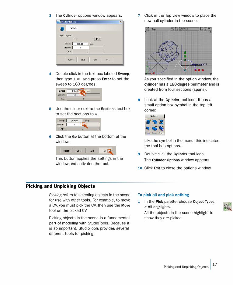
3 The Cylinder options window appears.
4 Double click in the text box labeled Sweep, then type 180 and press Enter to set the sweep to 180 degrees.
5 Use the slider next to the Sections text box to set the sections to 4.
6 Click the Go button at the bottom of the window.
This button applies the settings in the window and activates the tool.
7 Click in the Top view window to place the new half-cylinder in the scene.
As you specified in the option window, the cylinder has a 180-degree perimeter and is created from four sections (spans).
8 Look at the Cylinder tool icon. It has a small option box symbol in the top left corner.
Like the symbol in the menu, this indicates the tool has options.
9 Double-click the Cylinder tool icon.The Cylinder Options window appears.
10 Click Exit to close the options window.
Picking and Unpicking Objects
Picking refers to selecting objects in the scene for use with other tools. For example, to move a CV, you must pick the CV, then use the Move tool on the picked CV.
Picking objects in the scene is a fundamental part of modeling with StudioTools. Because it is so important, StudioTools provides several different tools for picking.
To pick all and pick nothing
1 In the Pick palette, choose Object Types > All obj/lights.All the objects in the scene highlight to show they are picked.
17Picking and Unpicking Objects
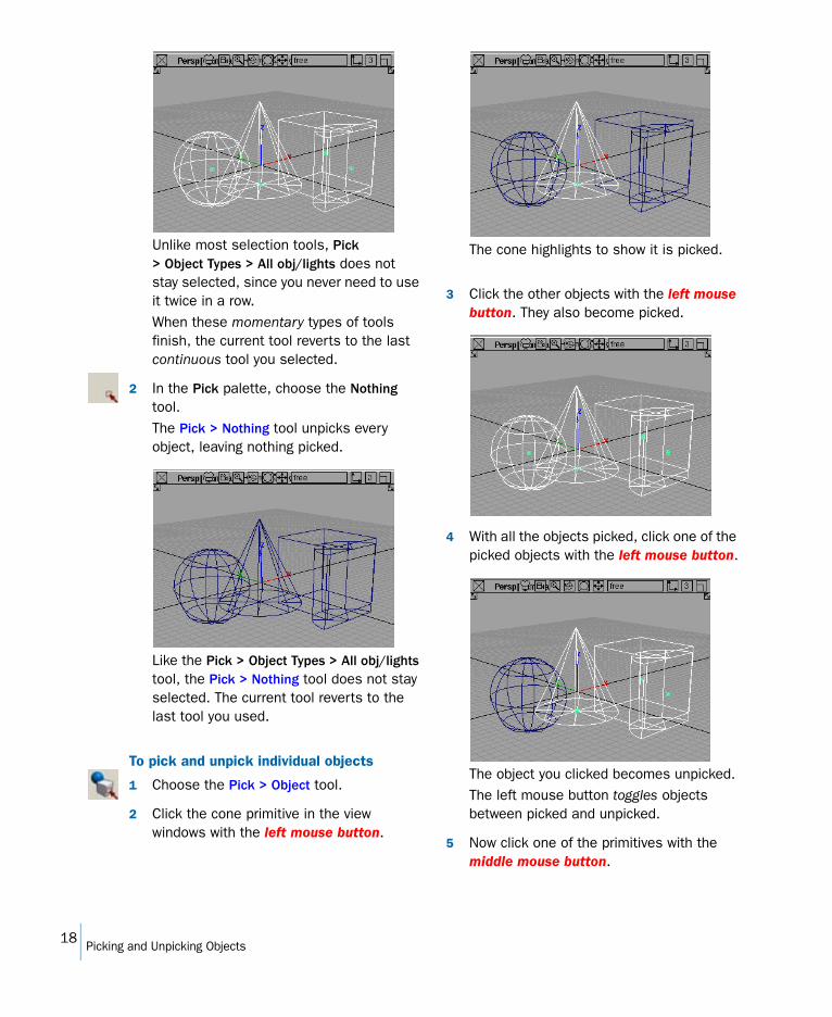
Unlike most selection tools, Pick > Object Types > All obj/lights does not stay selected, since you never need to use it twice in a row.When these momentary types of tools finish, the current tool reverts to the last continuous tool you selected.
2 In the Pick palette, choose the Nothing tool.The Pick > Nothing tool unpicks every object, leaving nothing picked.
Like the Pick > Object Types > All obj/lights tool, the Pick > Nothing tool does not stay selected. The current tool reverts to the last tool you used.
To pick and unpick individual objects
1 Choose the Pick > Object tool.
2 Click the cone primitive in the view windows with the left mouse button.
The cone highlights to show it is picked.
3 Click the other objects with the left mouse button. They also become picked.
4 With all the objects picked, click one of the picked objects with the left mouse button.
The object you clicked becomes unpicked.The left mouse button toggles objects between picked and unpicked.
5 Now click one of the primitives with the middle mouse button.
18Picking and Unpicking Objects
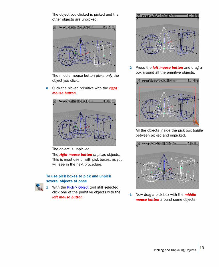
The object you clicked is picked and the other objects are unpicked.
The middle mouse button picks only the object you click.
6 Click the picked primitive with the right mouse button.
The object is unpicked.The right mouse button unpicks objects. This is most useful with pick boxes, as you will see in the next procedure.
To use pick boxes to pick and unpick several objects at once
1 With the Pick > Object tool still selected, click one of the primitive objects with the left mouse button.
2 Press the left mouse button and drag a box around all the primitive objects.
All the objects inside the pick box toggle between picked and unpicked.
3 Now drag a pick box with the middle mouse button around some objects.
19Picking and Unpicking Objects
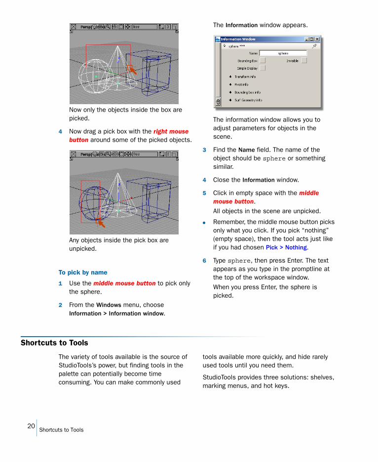
Now only the objects inside the box are picked.
4 Now drag a pick box with the right mouse button around some of the picked objects.
Any objects inside the pick box are unpicked.
To pick by name
1 Use the middle mouse button to pick only the sphere.
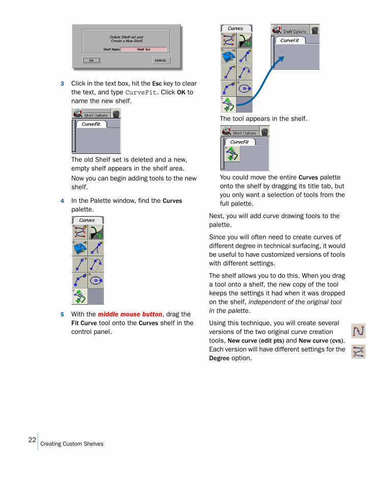
2 From the Windows menu, choose Information > Information window.
The Information window appears.
The information window allows you to adjust parameters for objects in the scene.
3 Find the Name field. The name of the object should be sphere or something similar.
4 Close the Information window.
5 Click in empty space with the middle mouse button.All objects in the scene are unpicked.
● Remember, the middle mouse button picks only what you click. If you pick “nothing” (empty space), then the tool acts just like if you had chosen Pick > Nothing.
6 Type sphere, then press Enter. The text appears as you type in the promptline at the top of the workspace window.When you press Enter, the sphere is picked.
Shortcuts to Tools
The variety of tools available is the source of StudioTools’s power, but finding tools in the palette can potentially become time consuming. You can make commonly used
tools available more quickly, and hide rarely used tools until you need them.
StudioTools provides three solutions: shelves, marking menus, and hot keys.
20Shortcuts to Tools

Shelves are like the palettes, except you control the tools’ options and their position on the shelves. You will use shelves to organize all your commonly used tools.
Marking menus pop-up at the current mouse location. They provide a very fast method to
choose the tools you use most often (such as Pick > Object).
Hot keys are special key combinations that perform common menu or tool commands.
Creating Custom Shelves
To show and hide the shelf window
1 In the Windows menu, choose Shelves.The Shelves window appears.
● The Shelves window provides a floating window in which to keep commonly used tools.StudioTools, however, provides another, even more convenient location for shelves. In these tutorials, you will use the shelf area in the control panel.
● Since you will not be using the Shelves window, you can close it.
2 Choose Windows > Shelves again to hide the Shelves window, or click the Shelves window’s close button.
To help demonstrate how to make new shelves, you will clear the default shelves and make new shelves specific to these tutorials.
Before you clear the default shelves, you will save them so you can retrieve them later.
To save the initial shelf set
1 Choose Windows > Control Panel. The control panel will appear.
2 Hold the left mouse button on the Shelf Options menu button at the top of the control panel’s shelf area to open the pop-up menu.
3 Drag down to the Save item and release the mouse button.A file requester appears.
4 Click in the File text field and type Default, then click Save.
In the next procedure, you will start a new shelf of tools commonly used in curve fitting in preparation for the lesson on fitting curves to scan data.
To clear the existing shelf set and create a new one
1 Hold the left mouse button on the menu button at the top of the shelf area to open the pop-up menu. Notice how the menu button is now called Default, after the name of the current shelf.
2 Choose New from the pop-up menu.A requester appears asking for the name of the new shelf.
21Creating Custom Shelves
3 Click in the text box, hit the Esc key to clear the text, and type CurveFit. Click OK to name the new shelf.
The old Shelf set is deleted and a new, empty shelf appears in the shelf area.Now you can begin adding tools to the new shelf.
4 In the Palette window, find the Curves palette.
5 With the middle mouse button, drag the Fit Curve tool onto the Curves shelf in the control panel.
The tool appears in the shelf.
You could move the entire Curves palette onto the shelf by dragging its title tab, but you only want a selection of tools from the full palette.
Next, you will add curve drawing tools to the palette.
Since you will often need to create curves of different degree in technical surfacing, it would be useful to have customized versions of tools with different settings.
The shelf allows you to do this. When you drag a tool onto a shelf, the new copy of the tool keeps the settings it had when it was dropped on the shelf, independent of the original tool in the palette.
Using this technique, you will create several versions of the two original curve creation tools, New curve (edit pts) and New curve (cvs). Each version will have different settings for the Degree option.
22Creating Custom Shelves
To add versions of the New Curve tools to the shelf with different options
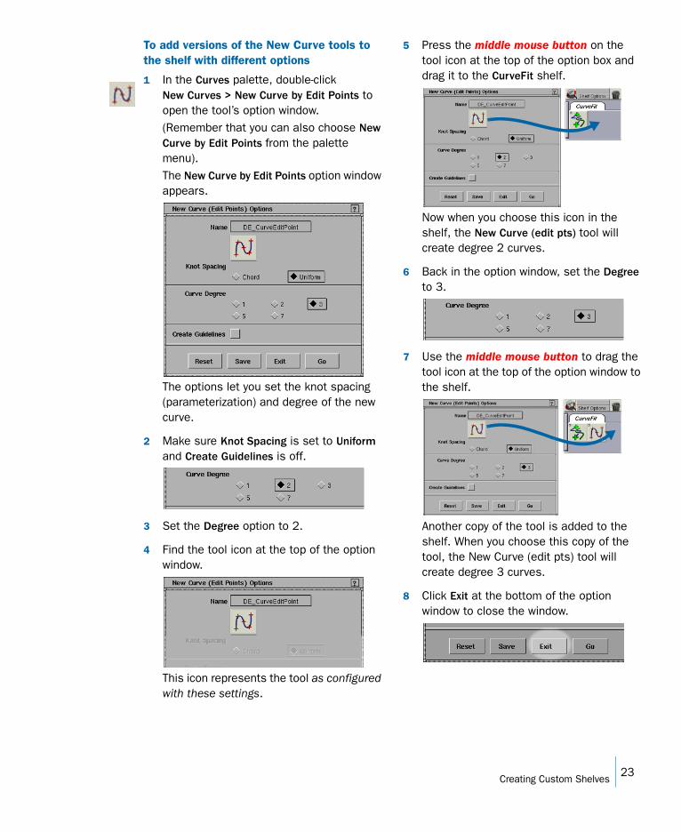
1 In the Curves palette, double-click New Curves > New Curve by Edit Points to open the tool’s option window.(Remember that you can also choose New Curve by Edit Points from the palette menu).The New Curve by Edit Points option window appears.
The options let you set the knot spacing (parameterization) and degree of the new curve.
2 Make sure Knot Spacing is set to Uniform and Create Guidelines is off.
3 Set the Degree option to 2.
4 Find the tool icon at the top of the option window.
This icon represents the tool as configured with these settings.
5 Press the middle mouse button on the tool icon at the top of the option box and drag it to the CurveFit shelf.
Now when you choose this icon in the shelf, the New Curve (edit pts) tool will create degree 2 curves.
6 Back in the option window, set the Degree to 3.
7 Use the middle mouse button to drag the tool icon at the top of the option window to the shelf.
Another copy of the tool is added to the shelf. When you choose this copy of the tool, the New Curve (edit pts) tool will create degree 3 curves.
8 Click Exit at the bottom of the option window to close the window.
23Creating Custom Shelves
To rename the tools
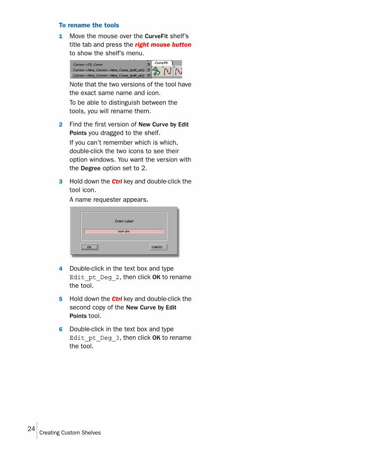
1 Move the mouse over the CurveFit shelf’s title tab and press the right mouse button to show the shelf’s menu.
Note that the two versions of the tool have the exact same name and icon.To be able to distinguish between the tools, you will rename them.
2 Find the first version of New Curve by Edit Points you dragged to the shelf.If you can’t remember which is which, double-click the two icons to see their option windows. You want the version with the Degree option set to 2.
3 Hold down the Ctrl key and double-click the tool icon.A name requester appears.
4 Double-click in the text box and type Edit_pt_Deg_2, then click OK to rename the tool.
5 Hold down the Ctrl key and double-click the second copy of the New Curve by Edit Points tool.
6 Double-click in the text box and type Edit_pt_Deg_3, then click OK to rename the tool.
24Creating Custom Shelves
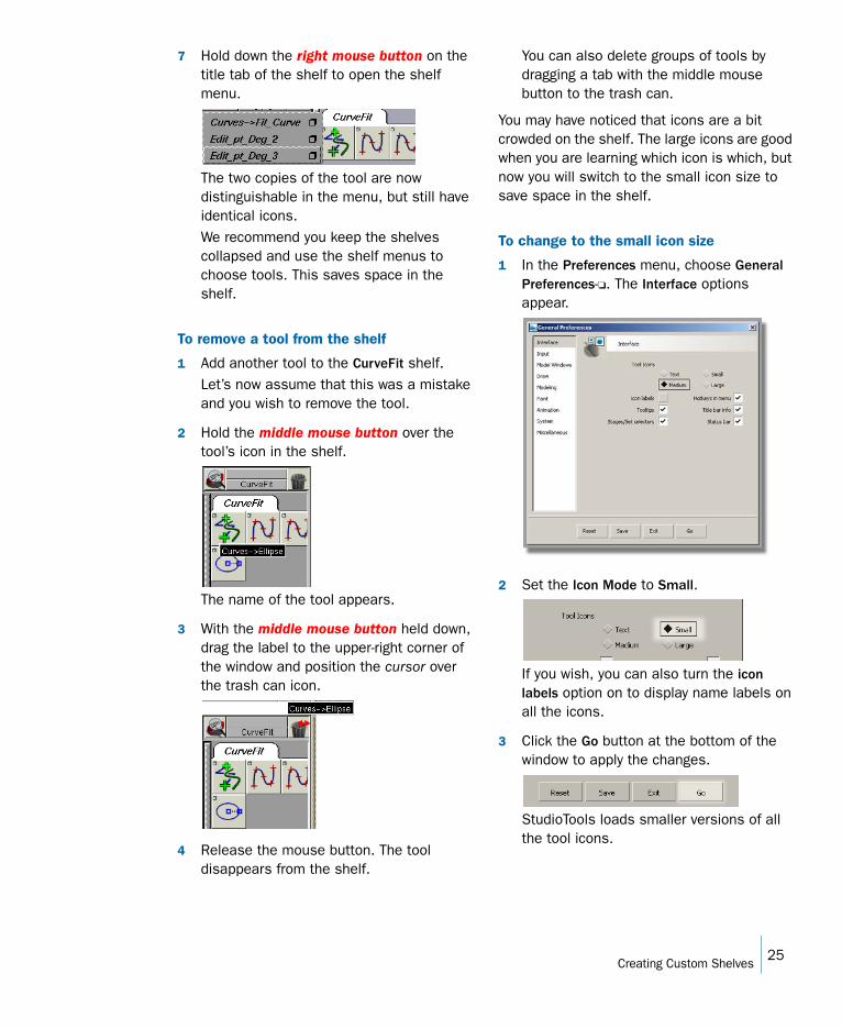
7 Hold down the right mouse button on the title tab of the shelf to open the shelf menu.
The two copies of the tool are now distinguishable in the menu, but still have identical icons.We recommend you keep the shelves collapsed and use the shelf menus to choose tools. This saves space in the shelf.
To remove a tool from the shelf
1 Add another tool to the CurveFit shelf.Let’s now assume that this was a mistake and you wish to remove the tool.
2 Hold the middle mouse button over the tool’s icon in the shelf.
The name of the tool appears.
3 With the middle mouse button held down, drag the label to the upper-right corner of the window and position the cursor over the trash can icon.
4 Release the mouse button. The tool disappears from the shelf.
You can also delete groups of tools by dragging a tab with the middle mouse button to the trash can.
You may have noticed that icons are a bit crowded on the shelf. The large icons are good when you are learning which icon is which, but now you will switch to the small icon size to save space in the shelf.
To change to the small icon size
1 In the Preferences menu, choose General Preferences-❏. The Interface options appear.
2 Set the Icon Mode to Small.
If you wish, you can also turn the icon labels option on to display name labels on all the icons.
3 Click the Go button at the bottom of the window to apply the changes.
StudioTools loads smaller versions of all the tool icons.
25Creating Custom Shelves

You have seen how to create shelves with customized tools. In later lessons you will load
pre-made shelves containing all the tools you need to complete the tutorials.
Using and Customizing Marking Menus
An even faster method for selecting tools are the marking menus. Marking menus generally hold fewer tools than a shelf, but are much faster since you can use quick gestures to choose tools. With practice, selecting tools with marking menus becomes almost instantaneous.
To choose common tools with marking menus
1 Hold down the Shift and Ctrl keys.
2 With the keys held down, hold the left mouse button.
The left mouse button marking menu appears at the location of the mouse pointer.
3 Keep the left mouse button held down and drag down until the Pick > Object box is highlighted.
A thick black line shows the direction of the mouse pointer.
4 Release the mouse button to choose the highlighted tool.The Pick > Object tool is now the current tool.
5 Hold Shift and Ctrl with the middle and then with the right mouse buttons to see the other marking menus.Each mouse button has a separate marking menu.
Once you have learned which direction corresponds to which tool in a marking menu, you can use a quick gesture to choose the tool.
6 Hold the Shift and Ctrl keys, then drag up and release the mouse button quickly.The black line shows the direction but the menu is not drawn.When you release the mouse button, the marking menu flashes the name of the selected tool on the screen.You have just selected Pick > Nothing.Use this method to choose tools even faster once you have mastered the positions of the tools on the menu.
Learn which tools are on the marking menus, and use the marking menus whenever you
Rightmousebutton
Middlemousebutton
26Using and Customizing Marking Menus
need to choose one of those tools. The more you use them, the faster you will become, until you can choose tools with quick gestures.
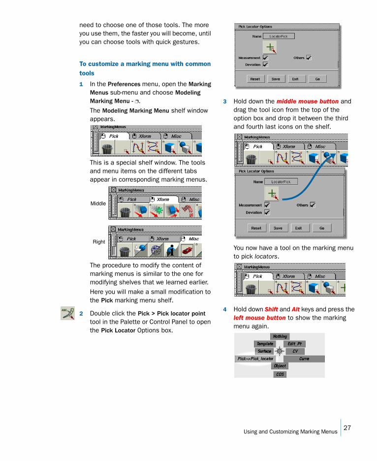
To customize a marking menu with common tools
1 In the Preferences menu, open the Marking Menus sub-menu and choose Modeling Marking Menu - ❐. The Modeling Marking Menu shelf window appears.
This is a special shelf window. The tools and menu items on the different tabs appear in corresponding marking menus.
The procedure to modify the content of marking menus is similar to the one for modifying shelves that we learned earlier. Here you will make a small modification to the Pick marking menu shelf.
2 Double click the Pick > Pick locator point tool in the Palette or Control Panel to open the Pick Locator Options box.
3 Hold down the middle mouse button and drag the tool icon from the top of the option box and drop it between the third and fourth last icons on the shelf.
You now have a tool on the marking menu to pick locators.
4 Hold down Shift and Alt keys and press the left mouse button to show the marking menu again.
Middle
Right
27Using and Customizing Marking Menus
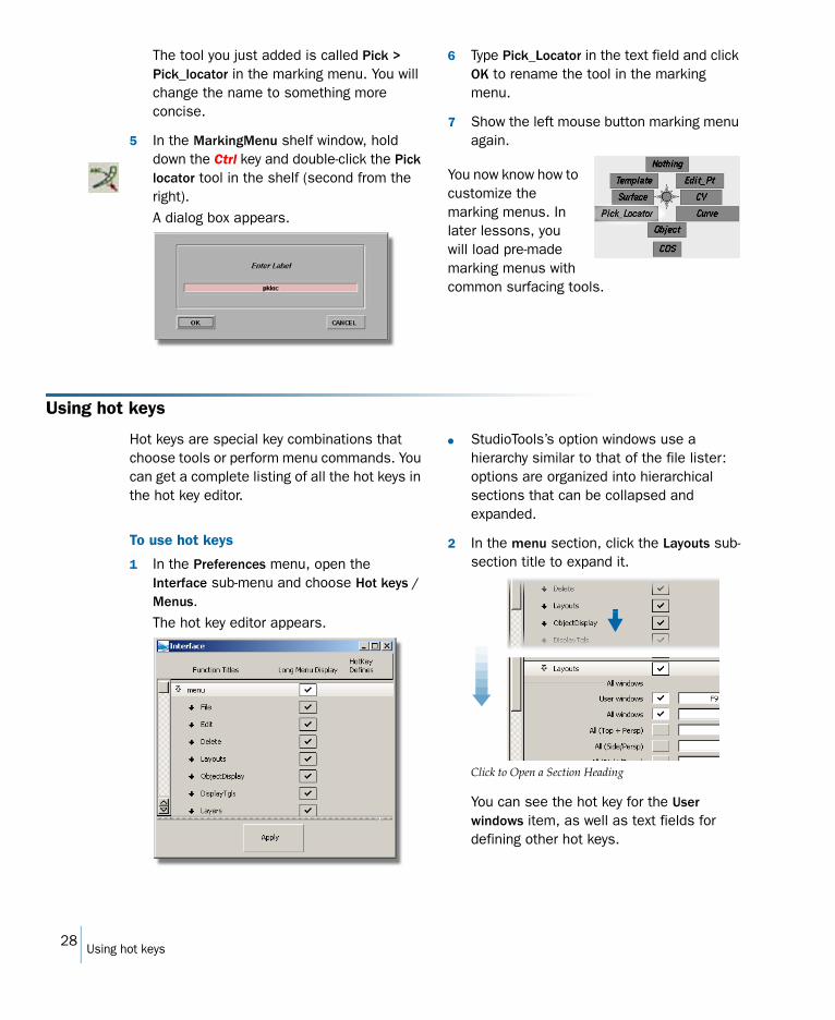
The tool you just added is called Pick > Pick_locator in the marking menu. You will change the name to something more concise.
5 In the MarkingMenu shelf window, hold down the Ctrl key and double-click the Pick locator tool in the shelf (second from the right).A dialog box appears.
6 Type Pick_Locator in the text field and click OK to rename the tool in the marking menu.
7 Show the left mouse button marking menu again.
You now know how to customize the marking menus. In later lessons, you will load pre-made marking menus with common surfacing tools.
Using hot keys
Hot keys are special key combinations that choose tools or perform menu commands. You can get a complete listing of all the hot keys in the hot key editor.
To use hot keys
1 In the Preferences menu, open the Interface sub-menu and choose Hot keys / Menus.The hot key editor appears.
● StudioTools’s option windows use a hierarchy similar to that of the file lister: options are organized into hierarchical sections that can be collapsed and expanded.
2 In the menu section, click the Layouts sub-section title to expand it.
Click to Open a Section Heading
You can see the hot key for the User windows item, as well as text fields for defining other hot keys.
28Using hot keys

You can define your own hot keys if you wish. For the most part we will not use hot keys in these lessons.If you are new to Alias StudioTools products, we recommend that you spend some time working with the product before you define hot keys, so you can learn which commands you use frequently enough to need a hot key.
3 Click the close box to close the hot key editor.
29Using hot keys
Changing Your View of the Model
Learn how StudioTools represents the 3D model on your 2D monitor, and how to use the
view controls to get the best possible angle on the model for the task at hand.
Tracking, Dollying, and Tumbling the Camera’s View
There are many different ways to change the camera’s view in StudioTools.
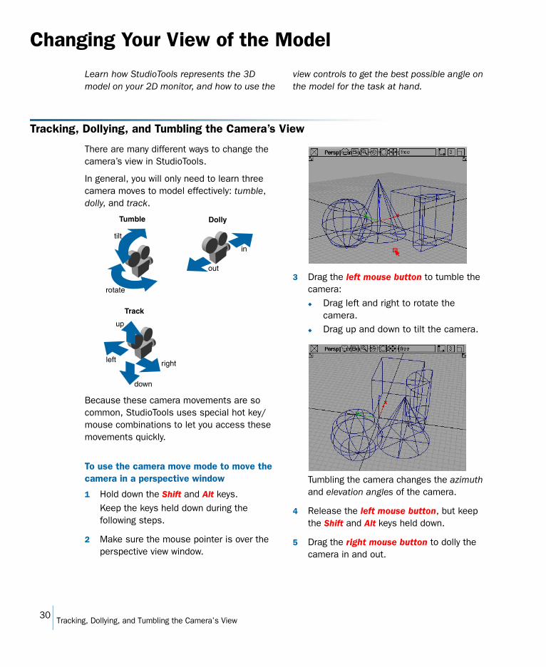
In general, you will only need to learn three camera moves to model effectively: tumble, dolly, and track.
Because these camera movements are so common, StudioTools uses special hot key/mouse combinations to let you access these movements quickly.
To use the camera move mode to move the camera in a perspective window
1 Hold down the Shift and Alt keys.Keep the keys held down during the following steps.
2 Make sure the mouse pointer is over the perspective view window.
3 Drag the left mouse button to tumble the camera:◆ Drag left and right to rotate the
camera.◆ Drag up and down to tilt the camera.
Tumbling the camera changes the azimuth and elevation angles of the camera.
4 Release the left mouse button, but keep the Shift and Alt keys held down.
5 Drag the right mouse button to dolly the camera in and out.
Dolly
in
out
Track
Tumble
rotate
tilt
up
down
left right
30Tracking, Dollying, and Tumbling the Camera’s View
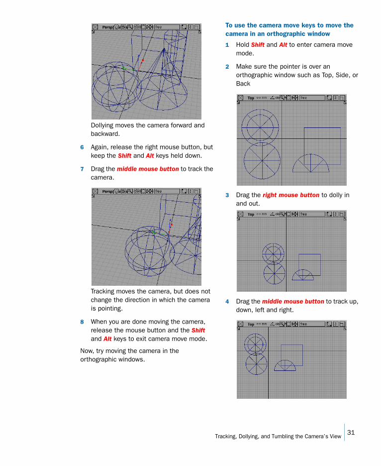
Dollying moves the camera forward and backward.
6 Again, release the right mouse button, but keep the Shift and Alt keys held down.
7 Drag the middle mouse button to track the camera.
Tracking moves the camera, but does not change the direction in which the camera is pointing.
8 When you are done moving the camera, release the mouse button and the Shift and Alt keys to exit camera move mode.
Now, try moving the camera in the orthographic windows.
To use the camera move keys to move the camera in an orthographic window
1 Hold Shift and Alt to enter camera move mode.
2 Make sure the pointer is over an orthographic window such as Top, Side, or Back
3 Drag the right mouse button to dolly in and out.
4 Drag the middle mouse button to track up, down, left and right.
31Tracking, Dollying, and Tumbling the Camera’s View
5 Now try dragging the left mouse button to tumble the orthographic view.Nothing happens. You cannot change the view direction of orthographic windows. They always look in the same direction.
Moving the camera is a very important skill in StudioTools. Throughout this book you will need to move the camera to work with geometry.
Using the camera move mode soon becomes second nature. With practice, you will be able to move the camera where you need it without thinking about the keys or the mouse.
Practice tumbling, tracking, and dollying the camera around the model some more before you move on.
To use Look At to center on an object
1 Use the marking menus to choose the Pick > Nothing tool.Remember that the left mouse button marking menu has the pick tools.
2 Now use the marking menus to choose the Pick > Object tool.
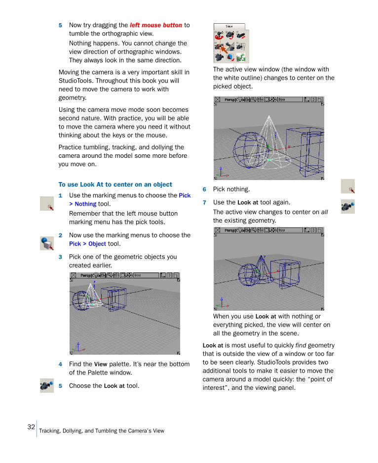
3 Pick one of the geometric objects you created earlier.
4 Find the View palette. It’s near the bottom of the Palette window.
5 Choose the Look at tool.
The active view window (the window with the white outline) changes to center on the picked object.
6 Pick nothing.
7 Use the Look at tool again.The active view changes to center on all the existing geometry.
When you use Look at with nothing or everything picked, the view will center on all the geometry in the scene.
Look at is most useful to quickly find geometry that is outside the view of a window or too far to be seen clearly. StudioTools provides two additional tools to make it easier to move the camera around a model quickly: the “point of interest”, and the viewing panel.
32Tracking, Dollying, and Tumbling the Camera’s View
Changing the Point of Interest
Normally, camera move mode (Shift+Alt) is calibrated to best view objects at the origin (the center of world space, coordinate 0,0,0). This can become awkward when you want to move the camera around objects away from the origin.
The point of interest manipulator lets you center the camera movements on a point on the model.
To use the point of interest manipulatorFirst, make sure the point of interest manipulator is turned on.
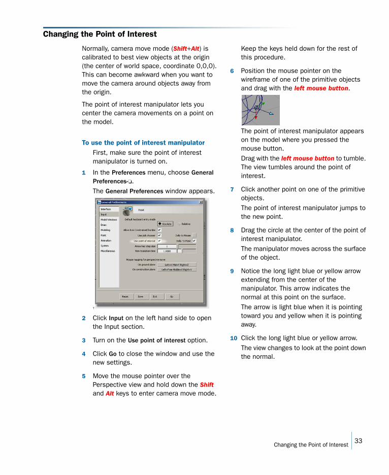
1 In the Preferences menu, choose General Preferences-❏. The General Preferences window appears.
T
2 Click Input on the left hand side to open the Input section.
3 Turn on the Use point of interest option.
4 Click Go to close the window and use the new settings.
5 Move the mouse pointer over the Perspective view and hold down the Shift and Alt keys to enter camera move mode.
Keep the keys held down for the rest of this procedure.
6 Position the mouse pointer on the wireframe of one of the primitive objects and drag with the left mouse button.
The point of interest manipulator appears on the model where you pressed the mouse button.Drag with the left mouse button to tumble. The view tumbles around the point of interest.
7 Click another point on one of the primitive objects.The point of interest manipulator jumps to the new point.
8 Drag the circle at the center of the point of interest manipulator.The manipulator moves across the surface of the object.
9 Notice the long light blue or yellow arrow extending from the center of the manipulator. This arrow indicates the normal at this point on the surface.The arrow is light blue when it is pointing toward you and yellow when it is pointing away.
10 Click the long light blue or yellow arrow.The view changes to look at the point down the normal.
33Changing the Point of Interest
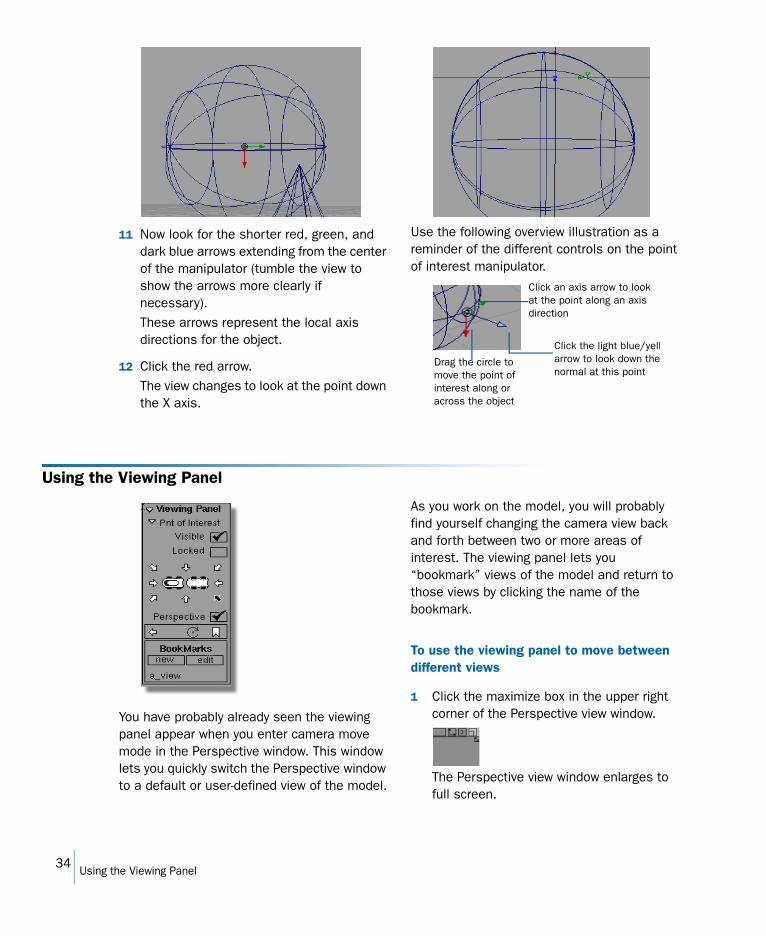
11 Now look for the shorter red, green, and dark blue arrows extending from the center of the manipulator (tumble the view to show the arrows more clearly if necessary).These arrows represent the local axis directions for the object.
12 Click the red arrow.The view changes to look at the point down the X axis.
Use the following overview illustration as a reminder of the different controls on the point of interest manipulator.
Using the Viewing Panel
You have probably already seen the viewing panel appear when you enter camera move mode in the Perspective window. This window lets you quickly switch the Perspective window to a default or user-defined view of the model.
As you work on the model, you will probably find yourself changing the camera view back and forth between two or more areas of interest. The viewing panel lets you “bookmark” views of the model and return to those views by clicking the name of the bookmark.
To use the viewing panel to move between different views
1 Click the maximize box in the upper right corner of the Perspective view window.
The Perspective view window enlarges to full screen.
Click an axis arrow to look at the point along an axis direction
Click the light blue/yellarrow to look down thenormal at this point
Drag the circle to move the point of interest along or across the object
34Using the Viewing Panel
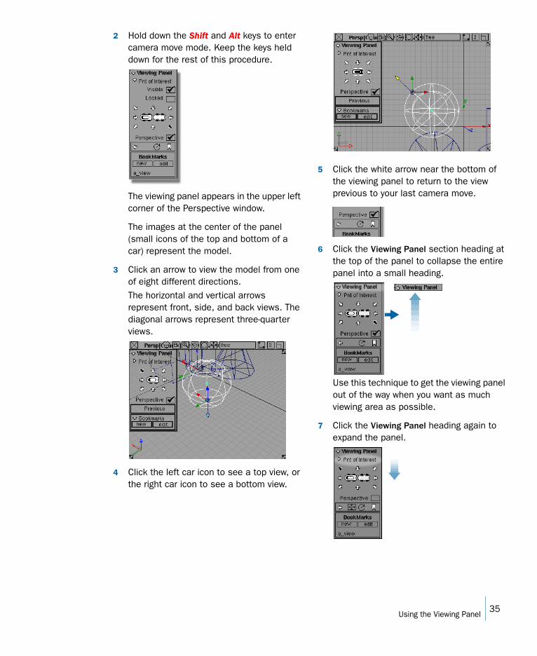
2 Hold down the Shift and Alt keys to enter camera move mode. Keep the keys held down for the rest of this procedure.
The viewing panel appears in the upper left corner of the Perspective window.
The images at the center of the panel (small icons of the top and bottom of a car) represent the model.
3 Click an arrow to view the model from one of eight different directions.The horizontal and vertical arrows represent front, side, and back views. The diagonal arrows represent three-quarter views.
4 Click the left car icon to see a top view, or the right car icon to see a bottom view.
5 Click the white arrow near the bottom of the viewing panel to return to the view previous to your last camera move.
6 Click the Viewing Panel section heading at the top of the panel to collapse the entire panel into a small heading.
Use this technique to get the viewing panel out of the way when you want as much viewing area as possible.
7 Click the Viewing Panel heading again to expand the panel.
35Using the Viewing Panel
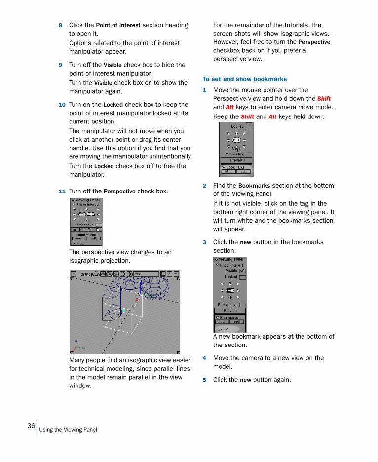
8 Click the Point of Interest section heading to open it.Options related to the point of interest manipulator appear.
9 Turn off the Visible check box to hide the point of interest manipulator.Turn the Visible check box on to show the manipulator again.
10 Turn on the Locked check box to keep the point of interest manipulator locked at its current position.The manipulator will not move when you click at another point or drag its center handle. Use this option if you find that you are moving the manipulator unintentionally.Turn the Locked check box off to free the manipulator.
11 Turn off the Perspective check box.
The perspective view changes to an isographic projection.
Many people find an isographic view easier for technical modeling, since parallel lines in the model remain parallel in the view window.
For the remainder of the tutorials, the screen shots will show isographic views. However, feel free to turn the Perspective checkbox back on if you prefer a perspective view.
To set and show bookmarks
1 Move the mouse pointer over the Perspective view and hold down the Shift and Alt keys to enter camera move mode.Keep the Shift and Alt keys held down.
2 Find the Bookmarks section at the bottom of the Viewing PanelIf it is not visible, click on the tag in the bottom right corner of the viewing panel. It will turn white and the bookmarks section will appear.
3 Click the new button in the bookmarks section.
A new bookmark appears at the bottom of the section.
4 Move the camera to a new view on the model.
5 Click the new button again.
mp
36Using the Viewing Panel

A second bookmark appears in the bookmark list.
6 Click the label for the first bookmark, then the second.The view switches back and forth between the two bookmarked views.
To be able to distinguish between bookmarks later, you should rename them now.
7 Click the edit button in the Bookmarks section.The Bookmark Lister window appears.
8 Release the Shift and Alt keys.
9 Hold down the Ctrl key and double-click the first bookmark icon in the Bookmark Lister.A dialog box appears.
10 Type a new name for the bookmark, then click OK.
For production work you should use meaningful names such as “back panel” or “door handle”.
By default, bookmarks are named BM, BM#2, BM#3, etc. Move the cursor over a bookmark icon to see its current name.
11 Ctrl double-click and rename the other bookmark.
12 Note the buttons in the Bookmark Lister window:◆ The Delete button removes the current
bookmark (green outline) from the list.◆ The New button adds a bookmark of
the current view. This is the same as clicking new in the viewing panel.
◆ The Prev and Next buttons change the view to the bookmark that precedes or follows the highlighted bookmark (green outline).
◆ Clicking on a bookmark icon changes the view to that bookmark. This is the same as clicking a bookmark in the viewing panel.
13 Close the Bookmark Lister.
14 Hold the Shift and Alt keys in the Perspective window to show the viewing panel.Notice your new names in the Bookmarks section.
Use the following overview illustration as a reminder of the different controls on the viewing panel.
Delete New Prev Next Bookmark icons
37Using the Viewing Panel
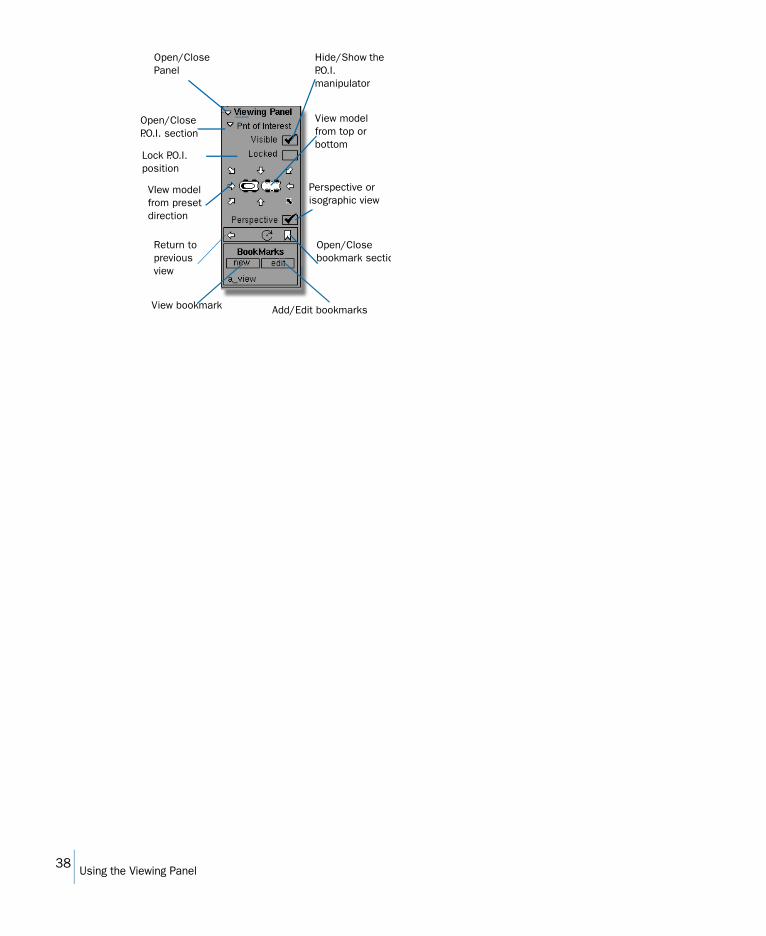
Open/Close Panel
Open/Close P.O.I. section
Lock P.O.I. position
Return to previous view
View bookmark
VIew model from preset direction
Hide/Show the P.O.I. manipulator
View model from top or bottom
Perspective or isographic view
Open/Close bookmark sectio
Add/Edit bookmarks
38Using the Viewing Panel
Understanding the object lister
StudioTools keeps track of every aspect of the scene in a hierarchical data structure. You can view representations of this structure through the SBD (scene block diagram) or through the object lister.
Curves, surfaces, groupings, transformations, components, lights, and everything else in the scene is represented by nodes in the hierarchy.
You may want to use the object lister in the following circumstances:
● In complex models, it can be easier to pick objects in the object lister than in a view window.
● The object lister shows important information that has no visual equivalent in the view windows, such as how the components and objects are grouped together, and how they relate to modeling layers.
● The object lister lets you confirm the effects of tools and menu items on the internal structure of the scene to help diagnose problems.
Types of Nodes
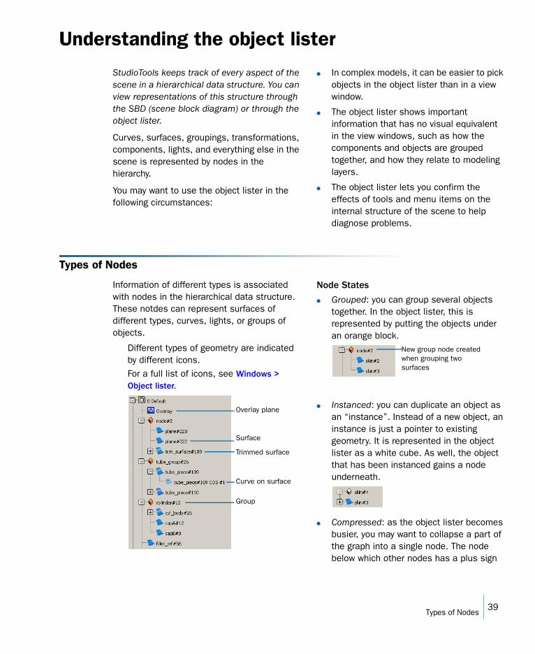
Information of different types is associated with nodes in the hierarchical data structure. These notdes can represent surfaces of different types, curves, lights, or groups of objects.
Different types of geometry are indicated by different icons.For a full list of icons, see Windows > Object lister.
Node States
● Grouped: you can group several objects together. In the object lister, this is represented by putting the objects under an orange block.
● Instanced: you can duplicate an object as an “instance”. Instead of a new object, an instance is just a pointer to existing geometry. It is represented in the object lister as a white cube. As well, the object that has been instanced gains a node underneath.
● Compressed: as the object lister becomes busier, you may want to collapse a part of the graph into a single node. The node below which other nodes has a plus sign
Overlay plane
Surface
Trimmed surface
Curve on surface
Group
New group node created when grouping two surfaces
39Types of Nodes
(+) in front of it. Nodes that have been expanded and can be collapsed have a minus sign (-) in front. Shift-click on a - or + sign to expand or compress the entire hierarchy.
● Invisible: you can make objects in the scene invisible. Nodes for invisible objects have gray text.
● Templated: you can “template” objects in the scene so that they are still visible, but cannot be transformed or picked. Nodes for templated objects do not change their appearance, but when the object is picked, it will be pink in the view windows, and its color when inactive is gray.
The Object lister window
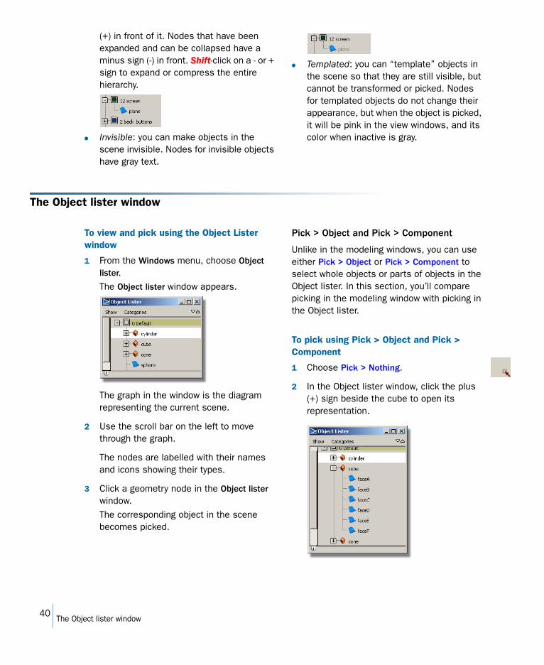
To view and pick using the Object Lister window
1 From the Windows menu, choose Object lister.The Object lister window appears.
The graph in the window is the diagram representing the current scene.
2 Use the scroll bar on the left to move through the graph.
The nodes are labelled with their names and icons showing their types.
3 Click a geometry node in the Object lister window.The corresponding object in the scene becomes picked.
Pick > Object and Pick > Component
Unlike in the modeling windows, you can use either Pick > Object or Pick > Component to select whole objects or parts of objects in the Object lister. In this section, you’ll compare picking in the modeling window with picking in the Object lister.
To pick using Pick > Object and Pick > Component
1 Choose Pick > Nothing.
2 In the Object lister window, click the plus (+) sign beside the cube to open its representation.
40The Object lister window
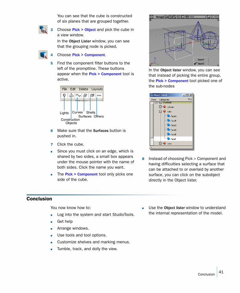
You can see that the cube is constructed of six planes that are grouped together.
3 Choose Pick > Object and pick the cube in a view window.In the Object Lister window, you can see that the grouping node is picked.
4 Choose Pick > Component.
5 Find the component filter buttons to the left of the promptline. These buttons appear when the Pick > Component tool is active.
6 Make sure that the Surfaces button is pushed in.
7 Click the cube.
● Since you must click on an edge, which is shared by two sides, a small box appears under the mouse pointer with the name of both sides. Click the name you want.
● The Pick > Component tool only picks one side of the cube.
In the Object lister window, you can see that instead of picking the entire group, the Pick > Component tool picked one of the sub-nodes.
8 Instead of choosing Pick > Component and having difficulties selecting a surface that can be attached to or overlaid by another surface, you can click on the subobject directly in the Object lister.
Conclusion
You now know how to:
● Log into the system and start StudioTools.
● Get help
● Arrange windows.
● Use tools and tool options.
● Customize shelves and marking menus.
● Tumble, track, and dolly the view.
● Use the Object lister window to understand the internal representation of the model.
CurvesSurfaces
ShellsOthers
Lights
Construction Objects
41Conclusion

42Conclusion

INTRODUCTION TO THE TUTORIAL
This section covers:
● Tutorial overview
● Prerequisites
● Introduction to surface modeling.
All of the tools and features required to perform this tutorial are available in SurfaceStudio and
AutoStudio, and may be available in Studio, depending on the options purchased.
This tutorial is intended for those users who want to learn surface modeling. In order to successfully complete this tutorial, we strongly recommend that you have a basic understanding of StudioTools. The ideal student for this tutorial will have completed all of the StudioTools basic tutorials, and have achieved, or have experience equal to, a Level 2 design status. SurfaceStudio 12 should be used to accompany this tutorial.
Upon completion of this tutorial, you will have an understanding of the following methods
● How to create curves and surfaces
● How to match curves and surfaces
● How to evaluate the finished model.
While this tutorial offers a recommended step-by-step strategy for surface modeling, other tools and methods will be addressed to show alternative methods and their associated errors.
Given that there are a number of strategies that can be employed to surface a model, the successful completion of a surface modeling project ultimately depends on a number of factors.
Key factors that contribute to a successful surface modeling project
● The software utilized to carry out the project
● The desired quality of the finished product
● The time allocated for the project.
An iterative method will be employed in this tutorial to detail the basic steps involved in surface modeling; however, it must be stated that you may eventually find a
5

methodology unique to your environment, or creative process, that works best for your requirements.
6

SOME COMMON MODELING BASICS
Learning Objectives
In this section you will learn how to:
● Set up the software to suit your working preferences
● The basic concepts of modeling.
Quality Defines the Model
Surface models can be constructed to meet a number of quality levels that depend on the intended purpose of the model and the time allotted for the project. For instance, a model that has to be milled immediately as a 1:4 scaled model will have a different design phase than a model of a digitized master that is intended for a major CAD system (such as CATIA, or Unigraphics).
Surface modeling quality levels
● Class A quality (sometimes referred to as Class 1)
● Class B quality
● Class C quality
Often, quality levels have no fixed definitions as companies often institute their own standards that reflect the demands of their particular industries. Details that are important to surface quality may include the use, or negation of, construction tolerances, highlight standards, trimmed surfaces, radii shape, flange availability, Bezier surfaces, and triangle surfaces.
In general, a surface modeling project can be defined by three questions.
1 Do the construction tolerances of the continuity between surfaces match the construction tolerances for the required data of the next step (CAD system, milling)?
2 Do the quality of highlights and curvature combs meet the requirements defined by the designer responsible for the model?
3 Do the data requirements of an external package match those used to create the model?
7
When working with SurfaceStudio, you should begin by setting the construction tolerances. The input construction tolerance levels will depend on the type of system employed to execute the design. If you do not know the
construction tolerances at the onset of your project, you can follow one simple rule.
Solid modeling systems (Pro/Engineer, SolidWorks) require small position construction tolerances. Ensure your construction tolerance values work with your solid modeling system.
How Different Types of Input Affect the Model
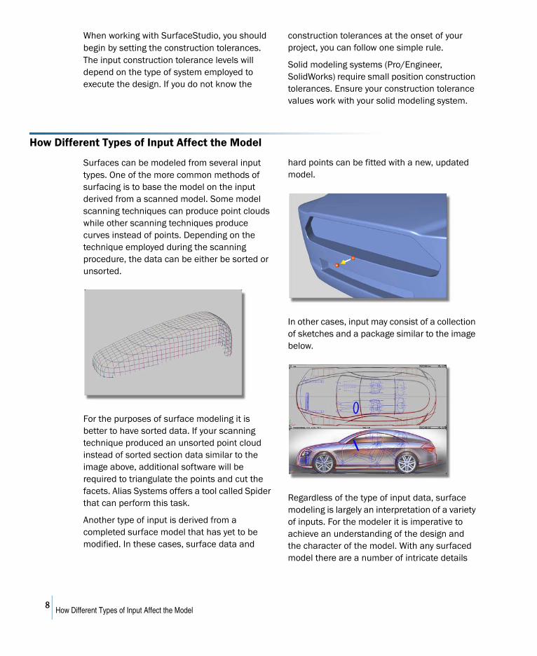
Surfaces can be modeled from several input types. One of the more common methods of surfacing is to base the model on the input derived from a scanned model. Some model scanning techniques can produce point clouds while other scanning techniques produce curves instead of points. Depending on the technique employed during the scanning procedure, the data can be either be sorted or unsorted.
For the purposes of surface modeling it is better to have sorted data. If your scanning technique produced an unsorted point cloud instead of sorted section data similar to the image above, additional software will be required to triangulate the points and cut the facets. Alias Systems offers a tool called Spider that can perform this task.
Another type of input is derived from a completed surface model that has yet to be modified. In these cases, surface data and
hard points can be fitted with a new, updated model.
In other cases, input may consist of a collection of sketches and a package similar to the image below.
Regardless of the type of input data, surface modeling is largely an interpretation of a variety of inputs. For the modeler it is imperative to achieve an understanding of the design and the character of the model. With any surfaced model there are a number of intricate details
8How Different Types of Input Affect the Model
that lay hidden below the surface, known only to the designer and modeler. Due to the precision of modeling software, the modeler must develop a close working relationship with
the designer in order to surface the model. After all, surface modeling is a creative process that finishes a design.
Loading and Organizing Data
To work with saved data, you must first load it into StudioTools. After you open the data you can organize it into layers, allowing you to manage it more efficiently.
In this lesson, we will show you how to work with SurfaceStudio files, open and organize files.
Opening the Lesson File
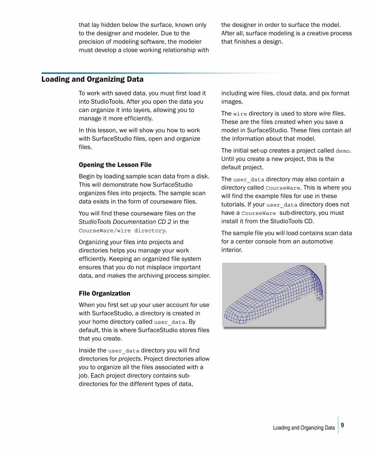
Begin by loading sample scan data from a disk. This will demonstrate how SurfaceStudio organizes files into projects. The sample scan data exists in the form of courseware files.
You will find these courseware files on the StudioTools Documentation CD 2 in the CourseWare/wire directory.
Organizing your files into projects and directories helps you manage your work efficiently. Keeping an organized file system ensures that you do not misplace important data, and makes the archiving process simpler.
File Organization
When you first set up your user account for use with SurfaceStudio, a directory is created in your home directory called user_data. By default, this is where SurfaceStudio stores files that you create.
Inside the user_data directory you will find directories for projects. Project directories allow you to organize all the files associated with a job. Each project directory contains sub-directories for the different types of data,
including wire files, cloud data, and pix format images.
The wire directory is used to store wire files. These are the files created when you save a model in SurfaceStudio. These files contain all the information about that model.
The initial set-up creates a project called demo. Until you create a new project, this is the default project.
The user_data directory may also contain a directory called CourseWare. This is where you will find the example files for use in these tutorials. If your user_data directory does not have a CourseWare sub-directory, you must install it from the StudioTools CD.
The sample file you will load contains scan data for a center console from an automotive interior.
9Loading and Organizing Data
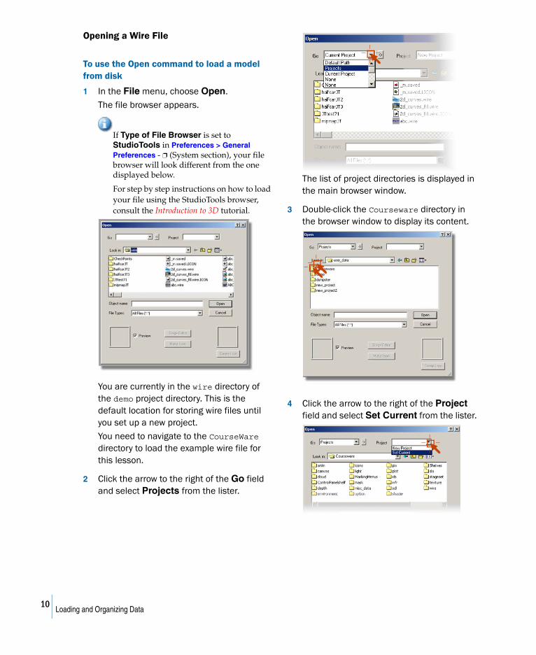
Opening a Wire File
To use the Open command to load a model from disk
1 In the File menu, choose Open.
The file browser appears.
If Type of File Browser is set to StudioTools in Preferences > General Preferences - ❐ (System section), your file browser will look different from the one displayed below.
For step by step instructions on how to load your file using the StudioTools browser, consult the Introduction to 3D tutorial.
You are currently in the wire directory of the demo project directory. This is the default location for storing wire files until you set up a new project.
You need to navigate to the CourseWare directory to load the example wire file for this lesson.
2 Click the arrow to the right of the Go field and select Projects from the lister.
The list of project directories is displayed in the main browser window.
3 Double-click the Courseware directory in the browser window to display its content.
4 Click the arrow to the right of the Project field and select Set Current from the lister.
10Loading and Organizing Data
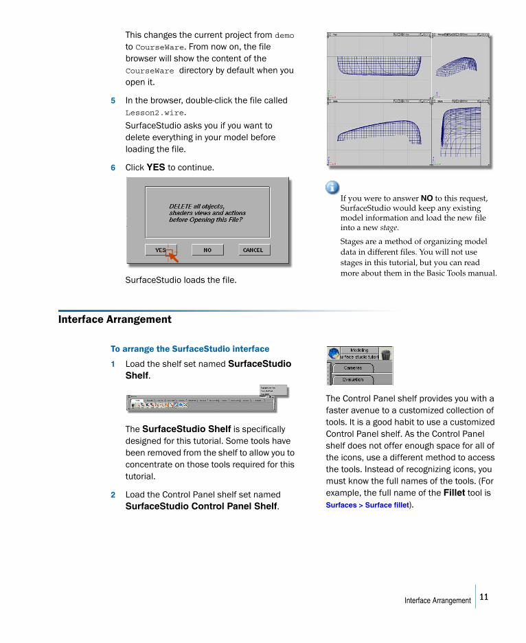
This changes the current project from demo to CourseWare. From now on, the file browser will show the content of the CourseWare directory by default when you open it.
5 In the browser, double-click the file called Lesson2.wire.
SurfaceStudio asks you if you want to delete everything in your model before loading the file.
6 Click YES to continue.
SurfaceStudio loads the file.
If you were to answer NO to this request, SurfaceStudio would keep any existing model information and load the new file into a new stage.
Stages are a method of organizing model data in different files. You will not use stages in this tutorial, but you can read more about them in the Basic Tools manual.
Interface Arrangement
To arrange the SurfaceStudio interface
1 Load the shelf set named SurfaceStudio Shelf.
The SurfaceStudio Shelf is specifically designed for this tutorial. Some tools have been removed from the shelf to allow you to concentrate on those tools required for this tutorial.
2 Load the Control Panel shelf set named SurfaceStudio Control Panel Shelf.
The Control Panel shelf provides you with a faster avenue to a customized collection of tools. It is a good habit to use a customized Control Panel shelf. As the Control Panel shelf does not offer enough space for all of the icons, use a different method to access the tools. Instead of recognizing icons, you must know the full names of the tools. (For example, the full name of the Fillet tool is Surfaces > Surface fillet).
11Interface Arrangement
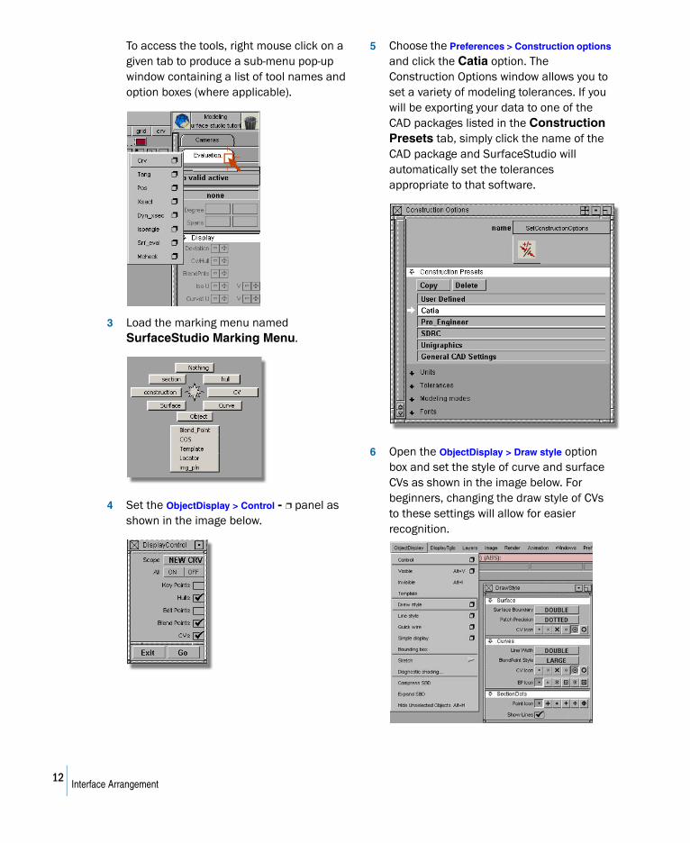
To access the tools, right mouse click on a given tab to produce a sub-menu pop-up window containing a list of tool names and option boxes (where applicable).
3 Load the marking menu named SurfaceStudio Marking Menu.
4 Set the ObjectDisplay > Control - ❐ panel as shown in the image below.
5 Choose the Preferences > Construction options and click the Catia option. The Construction Options window allows you to set a variety of modeling tolerances. If you will be exporting your data to one of the CAD packages listed in the Construction Presets tab, simply click the name of the CAD package and SurfaceStudio will automatically set the tolerances appropriate to that software.
6 Open the ObjectDisplay > Draw style option box and set the style of curve and surface CVs as shown in the image below. For beginners, changing the draw style of CVs to these settings will allow for easier recognition.
12Interface Arrangement
7 Save the selected options by choosing Preferences > User options > Save options from the menu.
8 Restart the computer to make sure your options are saved.
9 Open SurfaceStudio.
In this tutorial, the modeling process will be conducted solely in the Perspective view. You will be asked to change views in order to facilitate the best possible view of the model. For each instance when you are asked to change views, always use the Viewing Panel located in the Perspective window.
Traditional Surface Modeling
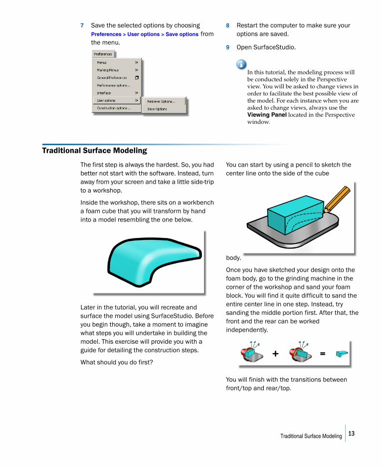
The first step is always the hardest. So, you had better not start with the software. Instead, turn away from your screen and take a little side-trip to a workshop.
Inside the workshop, there sits on a workbench a foam cube that you will transform by hand into a model resembling the one below.
Later in the tutorial, you will recreate and surface the model using SurfaceStudio. Before you begin though, take a moment to imagine what steps you will undertake in building the model. This exercise will provide you with a guide for detailing the construction steps.
What should you do first?
You can start by using a pencil to sketch the center line onto the side of the cube
body.
Once you have sketched your design onto the foam body, go to the grinding machine in the corner of the workshop and sand your foam block. You will find it quite difficult to sand the entire center line in one step. Instead, try sanding the middle portion first. After that, the front and the rear can be worked independently.
You will finish with the transitions between front/top and rear/top.
13Traditional Surface Modeling
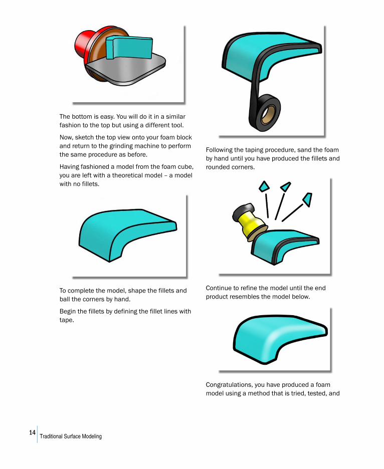
The bottom is easy. You will do it in a similar fashion to the top but using a different tool.
Now, sketch the top view onto your foam block and return to the grinding machine to perform the same procedure as before.
Having fashioned a model from the foam cube, you are left with a theoretical model – a model with no fillets.
To complete the model, shape the fillets and ball the corners by hand.
Begin the fillets by defining the fillet lines with tape.
Following the taping procedure, sand the foam by hand until you have produced the fillets and rounded corners.
Continue to refine the model until the end product resembles the model below.
Congratulations, you have produced a foam model using a method that is tried, tested, and
14Traditional Surface Modeling

true. As we step further into the tutorial, you will use this same classic method to develop your surface model.
15Traditional Surface Modeling

16Traditional Surface Modeling
CREATING AND FITTING CURVES
Learning Objectives
In this section you will learn how to:
● Create curves and fit them to the scan lines.
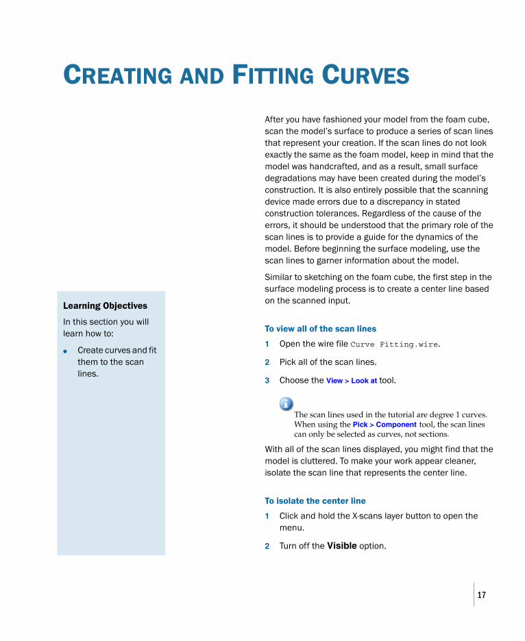
After you have fashioned your model from the foam cube, scan the model’s surface to produce a series of scan lines that represent your creation. If the scan lines do not look exactly the same as the foam model, keep in mind that the model was handcrafted, and as a result, small surface degradations may have been created during the model’s construction. It is also entirely possible that the scanning device made errors due to a discrepancy in stated construction tolerances. Regardless of the cause of the errors, it should be understood that the primary role of the scan lines is to provide a guide for the dynamics of the model. Before beginning the surface modeling, use the scan lines to garner information about the model.
Similar to sketching on the foam cube, the first step in the surface modeling process is to create a center line based on the scanned input.
To view all of the scan lines
1 Open the wire file Curve Fitting.wire.
2 Pick all of the scan lines.
3 Choose the View > Look at tool.
The scan lines used in the tutorial are degree 1 curves. When using the Pick > Component tool, the scan lines can only be selected as curves, not sections.
With all of the scan lines displayed, you might find that the model is cluttered. To make your work appear cleaner, isolate the scan line that represents the center line.
To isolate the center line
1 Click and hold the X-scans layer button to open the menu.
2 Turn off the Visible option.
17

3 Repeat Steps 1 and 2 for the Z-scans layer. In the end, only the Y-scan lines should remain visible.
4 Choose Pick > Object and select the scan line that represents the center line.
5 Choose ObjectDisplay > Hide Unselected. All unselected scan lines are hidden - only the selected center scan line is visible. (To make the hidden lines visible again, choose ObjectDisplay > Visible from the menu).
Commit these steps to memory – later in the tutorial you will be asked to isolate a particular scan line or make a layer visible or invisible.
You may recall that when you were in the workshop you found it difficult to shape the center line in one step. To complete the model, you shaped three main surfaces (the front, middle, and rear) and completed the model by adding two blends. Following the workshop example, fit a curve to the top part of the center scan line. Use an automatic fitting algorithm, such as the Curves > Text tool, to undertake this part of the project.
To fit the top part of the center line using the Curves > Fit Curve tool
1 In the Viewing Panel, switch to the side view by selecting the middle arrow in the bottom row of arrows.
2 Double-click the Curves > Text tool to produce the options box.
3 Select the scan line that represents the center line and set the options in the Fit Curve Control as shown in the image below.
The Curves > Text tool selects the entire scan line, but initially you will be interested in selecting only the top part of the curve.
4 Pick the cross that lies adjacent to the blue manipulator and move along the scan line until only the top portion of the curve is selected.
Your curve should resemble the above image. As you gain more experience with surface modeling, you will learn to judge the placement of the CVs. Later in the tutorial, the term “Hull / CV distribution” will be used to describe the placement of CVs.
18
By moving the crosses and changing the fitting method, you can influence the CV distribution.
Another method for achieving a good CV distribution is to pick the CVs and move them to the desired position. However, this method is not recommended at this point in the modeling process as moving CVs will destroy the construction history of the curve.
5 Repeat Steps 2 – 4 for the front and the rear portions of the center line.
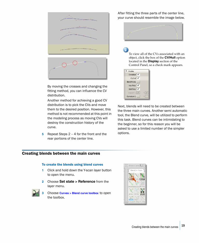
After fitting the three parts of the center line, your curve should resemble the image below.
To view all of the CVs associated with an object, click the box of the CV/Hull option located in the Display section of the Control Panel, so a check mark appears.
Next, blends will need to be created between the three main curves. Another semi automatic tool, the Blend curve, will be utilized to perform this task. Blend curves can be intimidating to the beginner, so for this reason you will be asked to use a limited number of the simpler options.
Creating blends between the main curves
To create the blends using blend curves
1 Click and hold down the Y-scan layer button to open the menu.
2 Choose Set state > Reference from the layer menu.
3 Choose Curves > Blend curve toolbox to open the toolbox.
19Creating blends between the main curves
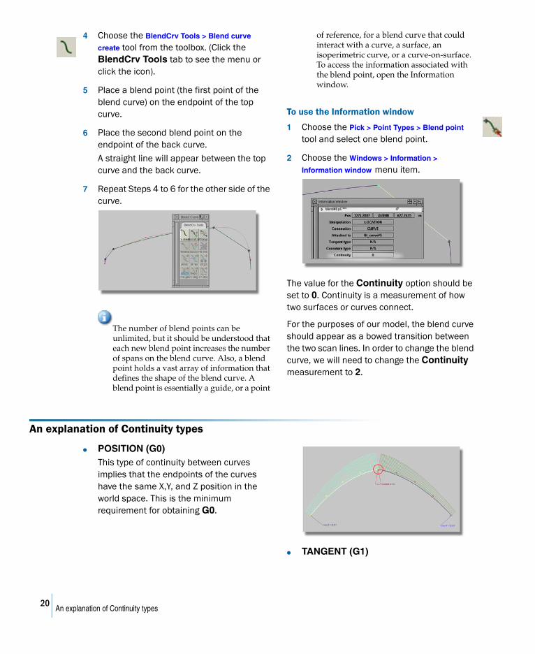
4 Choose the BlendCrv Tools > Blend curve
create tool from the toolbox. (Click the BlendCrv Tools tab to see the menu or click the icon).
5 Place a blend point (the first point of the blend curve) on the endpoint of the top curve.
6 Place the second blend point on the endpoint of the back curve.
A straight line will appear between the top curve and the back curve.
7 Repeat Steps 4 to 6 for the other side of the curve.
The number of blend points can be unlimited, but it should be understood that each new blend point increases the number of spans on the blend curve. Also, a blend point holds a vast array of information that defines the shape of the blend curve. A blend point is essentially a guide, or a point
of reference, for a blend curve that could interact with a curve, a surface, an isoperimetric curve, or a curve-on-surface. To access the information associated with the blend point, open the Information window.
To use the Information window
1 Choose the Pick > Point Types > Blend point tool and select one blend point.
2 Choose the Windows > Information >
Information window menu item.
The value for the Continuity option should be set to 0. Continuity is a measurement of how two surfaces or curves connect.
For the purposes of our model, the blend curve should appear as a bowed transition between the two scan lines. In order to change the blend curve, we will need to change the Continuity measurement to 2.
An explanation of Continuity types
● POSITION (G0)This type of continuity between curves implies that the endpoints of the curves have the same X,Y, and Z position in the world space. This is the minimum requirement for obtaining G0.
● TANGENT (G1)
20An explanation of Continuity types
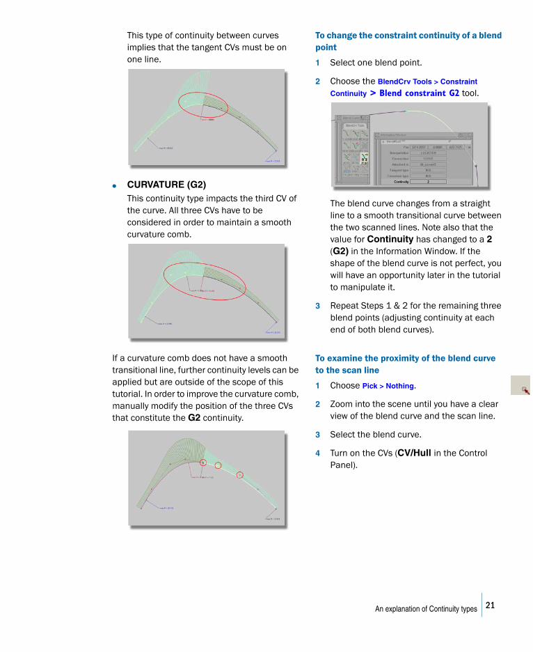
This type of continuity between curves implies that the tangent CVs must be on one line.
● CURVATURE (G2)This continuity type impacts the third CV of the curve. All three CVs have to be considered in order to maintain a smooth curvature comb.
If a curvature comb does not have a smooth transitional line, further continuity levels can be applied but are outside of the scope of this tutorial. In order to improve the curvature comb, manually modify the position of the three CVs that constitute the G2 continuity.
To change the constraint continuity of a blend point
1 Select one blend point.
2 Choose the BlendCrv Tools > Constraint
Continuity > Blend constraint G2 tool.
The blend curve changes from a straight line to a smooth transitional curve between the two scanned lines. Note also that the value for Continuity has changed to a 2 (G2) in the Information Window. If the shape of the blend curve is not perfect, you will have an opportunity later in the tutorial to manipulate it.
3 Repeat Steps 1 & 2 for the remaining three blend points (adjusting continuity at each end of both blend curves).
To examine the proximity of the blend curve to the scan line
1 Choose Pick > Nothing.
2 Zoom into the scene until you have a clear view of the blend curve and the scan line.
3 Select the blend curve.
4 Turn on the CVs (CV/Hull in the Control Panel).
21An explanation of Continuity types
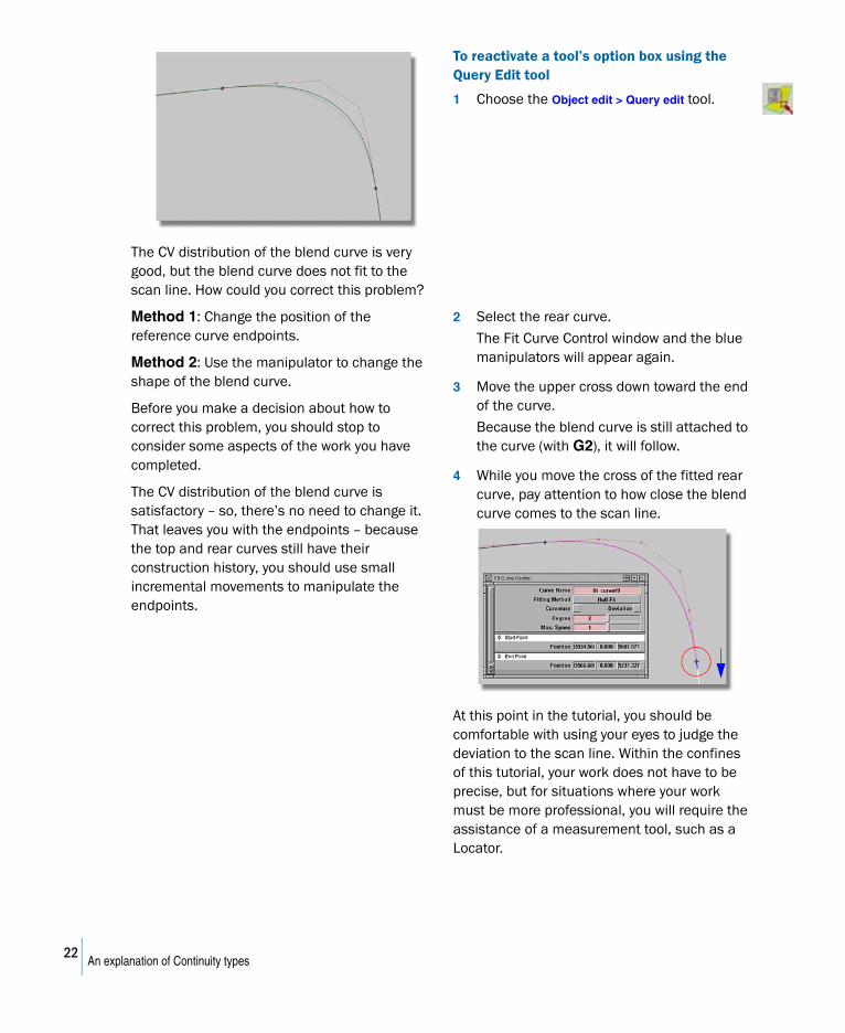
The CV distribution of the blend curve is very good, but the blend curve does not fit to the scan line. How could you correct this problem?
Method 1: Change the position of the reference curve endpoints.
Method 2: Use the manipulator to change the shape of the blend curve.
Before you make a decision about how to correct this problem, you should stop to consider some aspects of the work you have completed.
The CV distribution of the blend curve is satisfactory – so, there’s no need to change it. That leaves you with the endpoints – because the top and rear curves still have their construction history, you should use small incremental movements to manipulate the endpoints.
To reactivate a tool’s option box using the Query Edit tool
1 Choose the Object edit > Query edit tool.
2 Select the rear curve.
The Fit Curve Control window and the blue manipulators will appear again.
3 Move the upper cross down toward the end of the curve.
Because the blend curve is still attached to the curve (with G2), it will follow.
4 While you move the cross of the fitted rear curve, pay attention to how close the blend curve comes to the scan line.
At this point in the tutorial, you should be comfortable with using your eyes to judge the deviation to the scan line. Within the confines of this tutorial, your work does not have to be precise, but for situations where your work must be more professional, you will require the assistance of a measurement tool, such as a Locator.
22An explanation of Continuity types
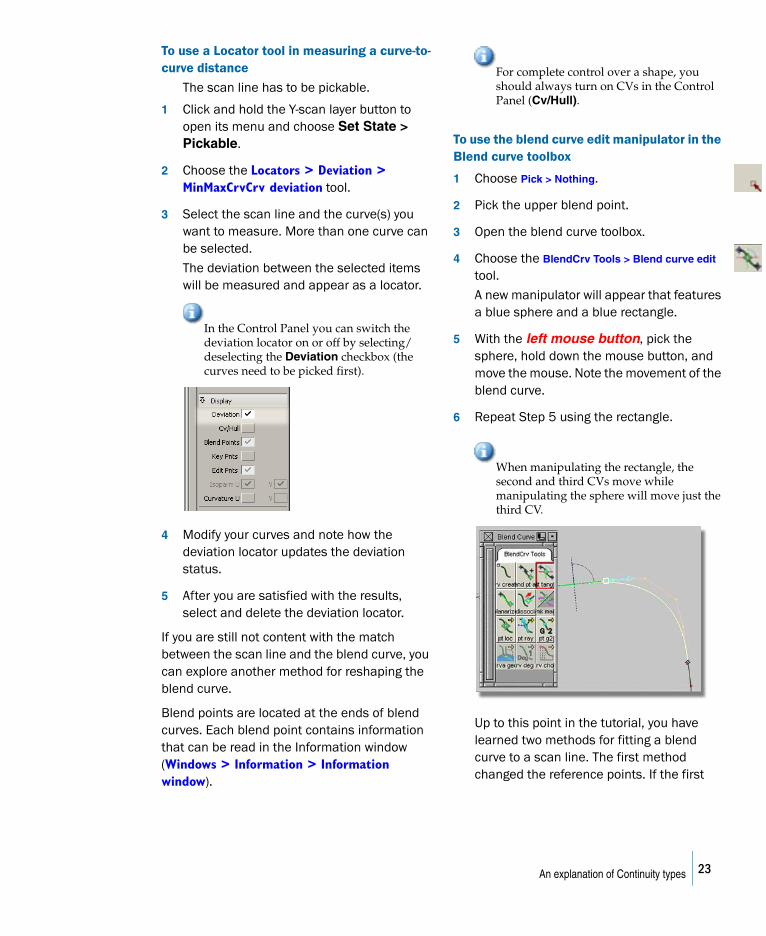
To use a Locator tool in measuring a curve-to-curve distance
The scan line has to be pickable.
1 Click and hold the Y-scan layer button to open its menu and choose Set State > Pickable.
2 Choose the Locators > Deviation > MinMaxCrvCrv deviation tool.
3 Select the scan line and the curve(s) you want to measure. More than one curve can be selected.
The deviation between the selected items will be measured and appear as a locator.
In the Control Panel you can switch the deviation locator on or off by selecting/deselecting the Deviation checkbox (the curves need to be picked first).
4 Modify your curves and note how the deviation locator updates the deviation status.
5 After you are satisfied with the results, select and delete the deviation locator.
If you are still not content with the match between the scan line and the blend curve, you can explore another method for reshaping the blend curve.
Blend points are located at the ends of blend curves. Each blend point contains information that can be read in the Information window (Windows > Information > Information window).
For complete control over a shape, you should always turn on CVs in the Control Panel (Cv/Hull).
To use the blend curve edit manipulator in the Blend curve toolbox
1 Choose Pick > Nothing.
2 Pick the upper blend point.
3 Open the blend curve toolbox.
4 Choose the BlendCrv Tools > Blend curve edit tool.
A new manipulator will appear that features a blue sphere and a blue rectangle.
5 With the left mouse button, pick the sphere, hold down the mouse button, and move the mouse. Note the movement of the blend curve.
6 Repeat Step 5 using the rectangle.
When manipulating the rectangle, the second and third CVs move while manipulating the sphere will move just the third CV.
Up to this point in the tutorial, you have learned two methods for fitting a blend curve to a scan line. The first method changed the reference points. If the first
23An explanation of Continuity types
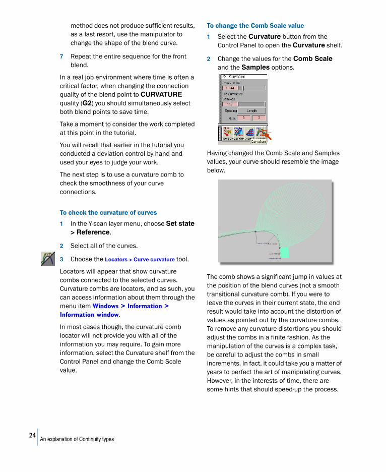
method does not produce sufficient results, as a last resort, use the manipulator to change the shape of the blend curve.
7 Repeat the entire sequence for the front blend.
In a real job environment where time is often a critical factor, when changing the connection quality of the blend point to CURVATURE quality (G2) you should simultaneously select both blend points to save time.
Take a moment to consider the work completed at this point in the tutorial.
You will recall that earlier in the tutorial you conducted a deviation control by hand and used your eyes to judge your work.
The next step is to use a curvature comb to check the smoothness of your curve connections.
To check the curvature of curves
1 In the Y-scan layer menu, choose Set state > Reference.
2 Select all of the curves.
3 Choose the Locators > Curve curvature tool.
Locators will appear that show curvature combs connected to the selected curves. Curvature combs are locators, and as such, you can access information about them through the menu item Windows > Information > Information window.
In most cases though, the curvature comb locator will not provide you with all of the information you may require. To gain more information, select the Curvature shelf from the Control Panel and change the Comb Scale value.
To change the Comb Scale value
1 Select the Curvature button from the Control Panel to open the Curvature shelf.
2 Change the values for the Comb Scale and the Samples options.
Having changed the Comb Scale and Samples values, your curve should resemble the image below.
The comb shows a significant jump in values at the position of the blend curves (not a smooth transitional curvature comb). If you were to leave the curves in their current state, the end result would take into account the distortion of values as pointed out by the curvature combs. To remove any curvature distortions you should adjust the combs in a finite fashion. As the manipulation of the curves is a complex task, be careful to adjust the combs in small increments. In fact, it could take you a matter of years to perfect the art of manipulating curves. However, in the interests of time, there are some hints that should speed-up the process.
24An explanation of Continuity types
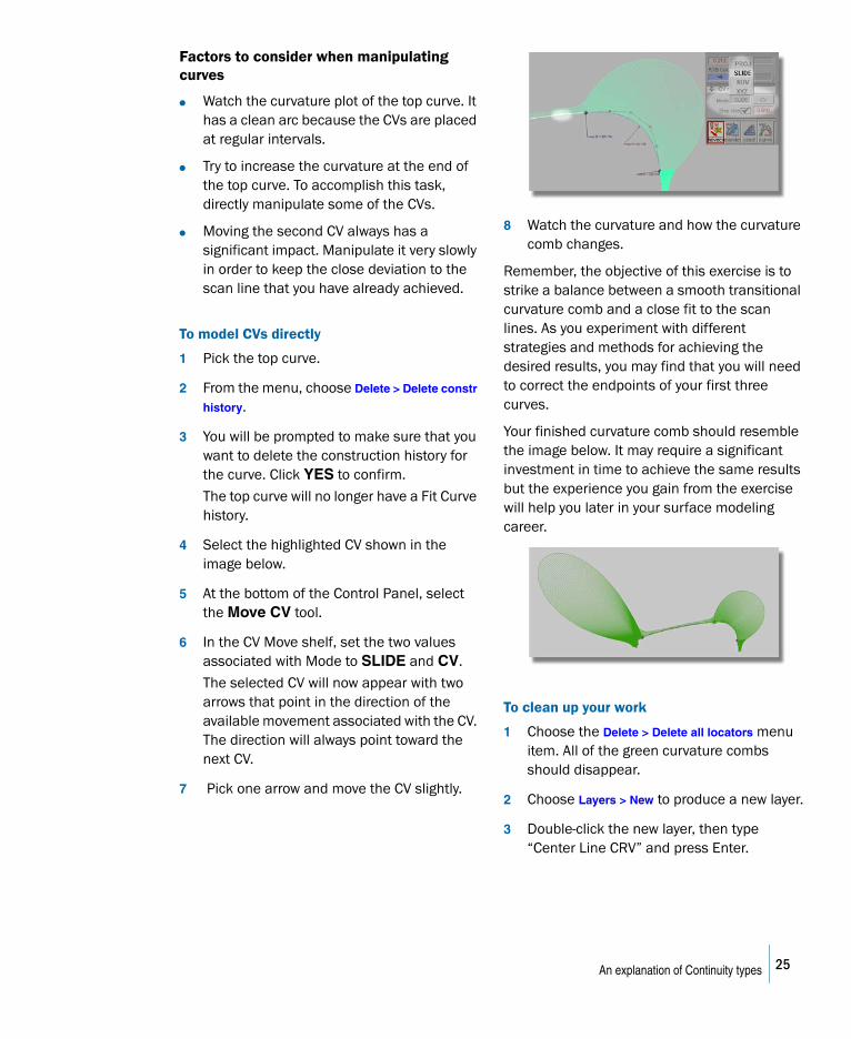
Factors to consider when manipulating curves
● Watch the curvature plot of the top curve. It has a clean arc because the CVs are placed at regular intervals.
● Try to increase the curvature at the end of the top curve. To accomplish this task, directly manipulate some of the CVs.
● Moving the second CV always has a significant impact. Manipulate it very slowly in order to keep the close deviation to the scan line that you have already achieved.
To model CVs directly
1 Pick the top curve.
2 From the menu, choose Delete > Delete constr
history.
3 You will be prompted to make sure that you want to delete the construction history for the curve. Click YES to confirm.
The top curve will no longer have a Fit Curve history.
4 Select the highlighted CV shown in the image below.
5 At the bottom of the Control Panel, select the Move CV tool.
6 In the CV Move shelf, set the two values associated with Mode to SLIDE and CV.
The selected CV will now appear with two arrows that point in the direction of the available movement associated with the CV. The direction will always point toward the next CV.
7 Pick one arrow and move the CV slightly.
8 Watch the curvature and how the curvature comb changes.
Remember, the objective of this exercise is to strike a balance between a smooth transitional curvature comb and a close fit to the scan lines. As you experiment with different strategies and methods for achieving the desired results, you may find that you will need to correct the endpoints of your first three curves.
Your finished curvature comb should resemble the image below. It may require a significant investment in time to achieve the same results but the experience you gain from the exercise will help you later in your surface modeling career.
To clean up your work
1 Choose the Delete > Delete all locators menu item. All of the green curvature combs should disappear.
2 Choose Layers > New to produce a new layer.
3 Double-click the new layer, then type “Center Line CRV” and press Enter.
25An explanation of Continuity types
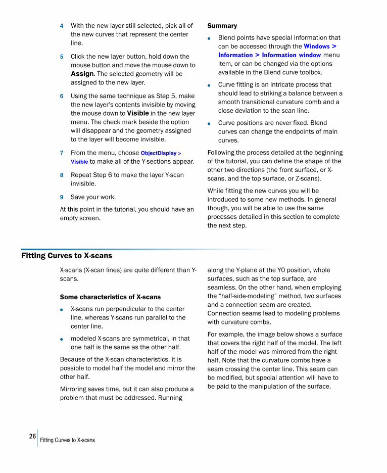
4 With the new layer still selected, pick all of the new curves that represent the center line.
5 Click the new layer button, hold down the mouse button and move the mouse down to Assign. The selected geometry will be assigned to the new layer.
6 Using the same technique as Step 5, make the new layer’s contents invisible by moving the mouse down to Visible in the new layer menu. The check mark beside the option will disappear and the geometry assigned to the layer will become invisible.
7 From the menu, choose ObjectDisplay >
Visible to make all of the Y-sections appear.
8 Repeat Step 6 to make the layer Y-scan invisible.
9 Save your work.
At this point in the tutorial, you should have an empty screen.
Summary
● Blend points have special information that can be accessed through the Windows > Information > Information window menu item, or can be changed via the options available in the Blend curve toolbox.
● Curve fitting is an intricate process that should lead to striking a balance between a smooth transitional curvature comb and a close deviation to the scan line.
● Curve positions are never fixed. Blend curves can change the endpoints of main curves.
Following the process detailed at the beginning of the tutorial, you can define the shape of the other two directions (the front surface, or X- scans, and the top surface, or Z-scans).
While fitting the new curves you will be introduced to some new methods. In general though, you will be able to use the same processes detailed in this section to complete the next step.
Fitting Curves to X-scans
X-scans (X-scan lines) are quite different than Y-scans.
Some characteristics of X-scans
● X-scans run perpendicular to the center line, whereas Y-scans run parallel to the center line.
● modeled X-scans are symmetrical, in that one half is the same as the other half.
Because of the X-scan characteristics, it is possible to model half the model and mirror the other half.
Mirroring saves time, but it can also produce a problem that must be addressed. Running
along the Y-plane at the Y0 position, whole surfaces, such as the top surface, are seamless. On the other hand, when employing the “half-side-modeling” method, two surfaces and a connection seam are created. Connection seams lead to modeling problems with curvature combs.
For example, the image below shows a surface that covers the right half of the model. The left half of the model was mirrored from the right half. Note that the curvature combs have a seam crossing the center line. This seam can be modified, but special attention will have to be paid to the manipulation of the surface.
26Fitting Curves to X-scans
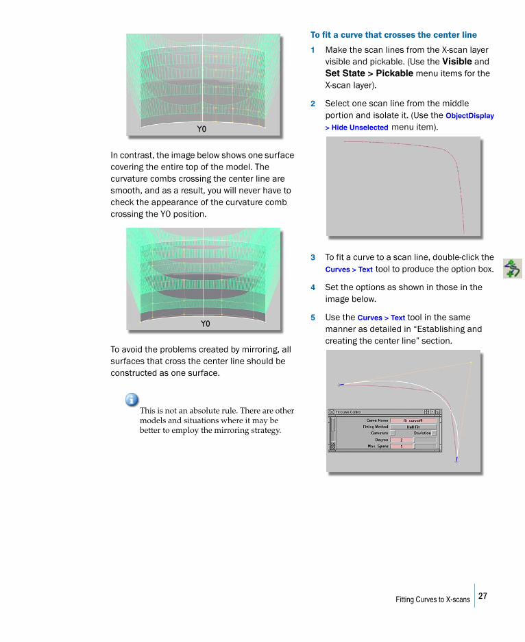
In contrast, the image below shows one surface covering the entire top of the model. The curvature combs crossing the center line are smooth, and as a result, you will never have to check the appearance of the curvature comb crossing the Y0 position.
To avoid the problems created by mirroring, all surfaces that cross the center line should be constructed as one surface.
This is not an absolute rule. There are other models and situations where it may be better to employ the mirroring strategy.
To fit a curve that crosses the center line
1 Make the scan lines from the X-scan layer visible and pickable. (Use the Visible and Set State > Pickable menu items for the X-scan layer).
2 Select one scan line from the middle portion and isolate it. (Use the ObjectDisplay
> Hide Unselected menu item).
3 To fit a curve to a scan line, double-click the Curves > Text tool to produce the option box.
4 Set the options as shown in those in the image below.
5 Use the Curves > Text tool in the same manner as detailed in “Establishing and creating the center line” section.
Y0
Y0
27Fitting Curves to X-scans
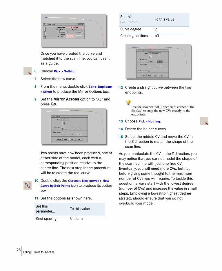
Once you have created the curve and matched it to the scan line, you can use it as a guide.
6 Choose Pick > Nothing.
7 Select the new curve.
8 From the menu, double-click Edit > Duplicate
> Mirror to produce the Mirror Options box.
9 Set the Mirror Across option to “XZ” and press Go.
Two points have now been produced, one at either side of the model, each with a corresponding position relative to the center line. The next step in the procedure will be to create the real curve.
10 Double-click the Curves > New curves > New
Curve by Edit Points icon to produce its option box.
11 Set the options as shown here.
12 Create a straight curve between the two endpoints.
Use the Magnet tool (upper right corner of the display) to snap the new CVs exactly to the endpoints.
13 Choose Pick > Nothing.
14 Delete the helper curves.
15 Select the middle CV and move the CV in the Z-direction to match the shape of the scan line.
As you manipulate the CV in the Z-direction, you may notice that you cannot model the shape of the scanned line with just one free CV. Eventually, you will need more CVs, but not before giving some thought to the maximum number of CVs you will require. To tackle this question, always start with the lowest degree (number of CVs) and increase the value in small steps. Employing a lowest-to-highest degree strategy should ensure that you do not overbuild your model.
Set this parameter...
To this value
Knot spacing Uniform
Curve degree 2
Create guidelines off
Set this parameter...
To this value
28Fitting Curves to X-scans
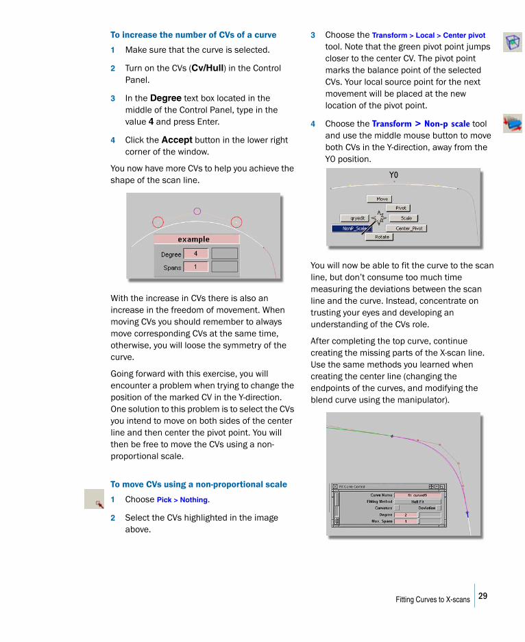
To increase the number of CVs of a curve
1 Make sure that the curve is selected.
2 Turn on the CVs (Cv/Hull) in the Control Panel.
3 In the Degree text box located in the middle of the Control Panel, type in the value 4 and press Enter.
4 Click the Accept button in the lower right corner of the window.
You now have more CVs to help you achieve the shape of the scan line.
With the increase in CVs there is also an increase in the freedom of movement. When moving CVs you should remember to always move corresponding CVs at the same time, otherwise, you will loose the symmetry of the curve.
Going forward with this exercise, you will encounter a problem when trying to change the position of the marked CV in the Y-direction. One solution to this problem is to select the CVs you intend to move on both sides of the center line and then center the pivot point. You will then be free to move the CVs using a non-proportional scale.
To move CVs using a non-proportional scale
1 Choose Pick > Nothing.
2 Select the CVs highlighted in the image above.
3 Choose the Transform > Local > Center pivot tool. Note that the green pivot point jumps closer to the center CV. The pivot point marks the balance point of the selected CVs. Your local source point for the next movement will be placed at the new location of the pivot point.
4 Choose the Transform > Non-p scale tool and use the middle mouse button to move both CVs in the Y-direction, away from the Y0 position.
You will now be able to fit the curve to the scan line, but don’t consume too much time measuring the deviations between the scan line and the curve. Instead, concentrate on trusting your eyes and developing an understanding of the CVs role.
After completing the top curve, continue creating the missing parts of the X-scan line. Use the same methods you learned when creating the center line (changing the endpoints of the curves, and modifying the blend curve using the manipulator).
Y0
29Fitting Curves to X-scans
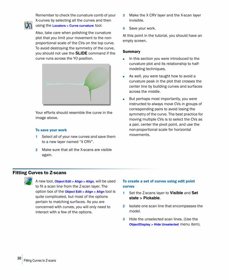
Remember to check the curvature comb of your X-curves by selecting all the curves and then using the Locators > Curve curvature tool.
Also, take care when polishing the curvature plot that you limit your movement to the non-proportional scale of the CVs on the top curve. To avoid destroying the symmetry of the curve, you should not use the SLIDE command if the curve runs across the Y0 position.
Your efforts should resemble the curve in the image above.
To save your work
1 Select all of your new curves and save them to a new layer named “X CRV”.
2 Make sure that all the X-scans are visible again.
3 Make the X CRV layer and the X-scan layer invisible.
4 Save your work.
At this point in the tutorial, you should have an empty screen.
Summary
● In this section you were introduced to the curvature plot and its relationship to half-modeling techniques.
● As well, you were taught how to avoid a curvature peak in the plot that crosses the center line by building curves and surfaces across the middle.
● But perhaps most importantly, you were instructed to always move CVs in groups of corresponding pairs to avoid losing the symmetry of the curve. The best practice for moving multiple CVs is to select the CVs as a pair, center the pivot point, and use the non-proportional scale for horizontal movements.
Fitting Curves to Z-scans
A new tool, Object Edit > Align > Align, will be used to fit a scan line from the Z-scan layer. The option box of the Object Edit > Align > Align tool is quite complicated, but most of the options pertain to matching surfaces. As you are concerned with curves, you will only need to interact with a few of the options.
To create a set of curves using edit point curves
1 Set the Z-scans layer to Visible and Set state > Pickable.
2 Isolate one scan line that encompasses the model.
3 Hide the unselected scan lines. (Use the ObjectDisplay > Hide Unselected menu item).
30Fitting Curves to Z-scans

4 Create a degree 2 edit point curve at the middle portion of the scan line by snapping the endpoints to the scan line. (Use the Curves > New curves > New Curve by Edit Points tool).
5 Pick the middle CVs and move the CVs in the Y-direction until you fit the shape of the scan line.
With flat shapes, you may find it difficult to judge the shape of your curve. To get a better view of your work, go to the Viewing Panel by pressing Shift + Alt. Inside the Viewing Panel, examine the four icons in the bottom rectangle. Make sure that the box beside the Perspective option does not contain a check mark. Inside the bottom rectangle, choose the square icon. You will now be able to dolly your view in a non-proportional manner that should provide for a better view of how your curve fits to the scan line.
To use the icons in the Viewing Panel
1 Press Shift + Alt and hold down the buttons.
2 Make sure that the Perspective option does not contain a check mark.
3 Choose the square icon. The icon will turn white to show that it is engaged.
4 Keep holding down the Shift + Alt keys. (The Viewing Panel must remain open to execute the view change).
5 Use the mouse buttons to scale the view.
The right mouse button scales the view both horizontally and vertically, the middle mouse button operates on the horizontal scale, and the left mouse button is reserved for the vertical scale.
6 To return to the original view, choose the Perspective option and then remove the check mark. The view should return to the natural scale in the orthographic view.
7 If the non-proportional view is not sufficient, choose the circled arrow icon at the bottom of the Viewing Panel to spin the view. To return to the original view, use the black arrows that surround the car icons in the middle of the Viewing Panel.
8 To fashion the front/rear curve, use the same technique employed on the X-scans.
Tips for creating a set of curves using edit point curves
● Use the Curves > Text tool.
31Fitting Curves to Z-scans
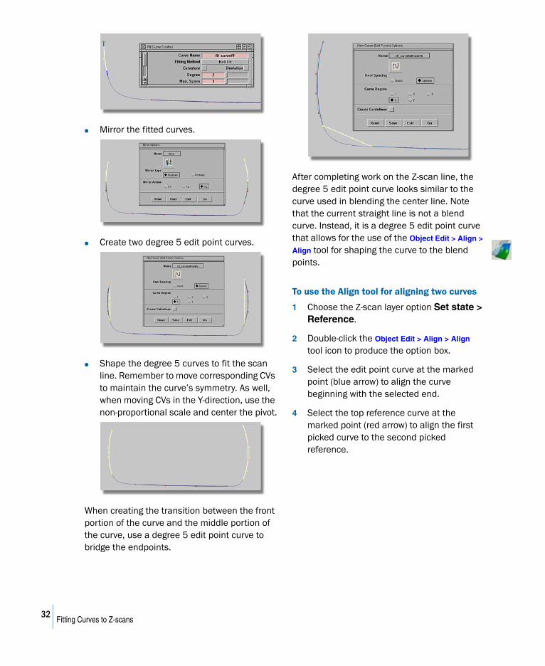
● Mirror the fitted curves.
● Create two degree 5 edit point curves.
● Shape the degree 5 curves to fit the scan line. Remember to move corresponding CVs to maintain the curve’s symmetry. As well, when moving CVs in the Y-direction, use the non-proportional scale and center the pivot.
When creating the transition between the front portion of the curve and the middle portion of the curve, use a degree 5 edit point curve to bridge the endpoints.
After completing work on the Z-scan line, the degree 5 edit point curve looks similar to the curve used in blending the center line. Note that the current straight line is not a blend curve. Instead, it is a degree 5 edit point curve that allows for the use of the Object Edit > Align >
Align tool for shaping the curve to the blend points.
To use the Align tool for aligning two curves
1 Choose the Z-scan layer option Set state > Reference.
2 Double-click the Object Edit > Align > Align tool icon to produce the option box.
3 Select the edit point curve at the marked point (blue arrow) to align the curve beginning with the selected end.
4 Select the top reference curve at the marked point (red arrow) to align the first picked curve to the second picked reference.
32Fitting Curves to Z-scans
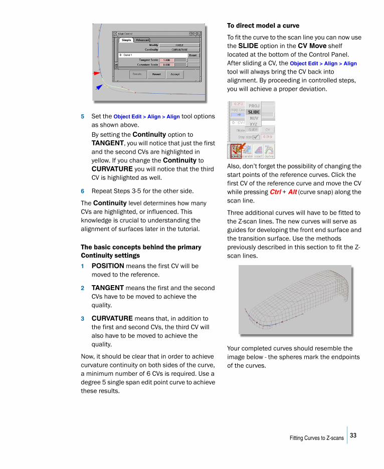
5 Set the Object Edit > Align > Align tool options as shown above.
By setting the Continuity option to TANGENT, you will notice that just the first and the second CVs are highlighted in yellow. If you change the Continuity to CURVATURE you will notice that the third CV is highlighted as well.
6 Repeat Steps 3-5 for the other side.
The Continuity level determines how many CVs are highlighted, or influenced. This knowledge is crucial to understanding the alignment of surfaces later in the tutorial.
The basic concepts behind the primary Continuity settings
1 POSITION means the first CV will be moved to the reference.
2 TANGENT means the first and the second CVs have to be moved to achieve the quality.
3 CURVATURE means that, in addition to the first and second CVs, the third CV will also have to be moved to achieve the quality.
Now, it should be clear that in order to achieve curvature continuity on both sides of the curve, a minimum number of 6 CVs is required. Use a degree 5 single span edit point curve to achieve these results.
To direct model a curve
To fit the curve to the scan line you can now use the SLIDE option in the CV Move shelf located at the bottom of the Control Panel. After sliding a CV, the Object Edit > Align > Align tool will always bring the CV back into alignment. By proceeding in controlled steps, you will achieve a proper deviation.
Also, don’t forget the possibility of changing the start points of the reference curves. Click the first CV of the reference curve and move the CV while pressing Ctrl + Alt (curve snap) along the scan line.
Three additional curves will have to be fitted to the Z-scan lines. The new curves will serve as guides for developing the front end surface and the transition surface. Use the methods previously described in this section to fit the Z-scan lines.
Your completed curves should resemble the image below - the spheres mark the endpoints of the curves.
33Fitting Curves to Z-scans
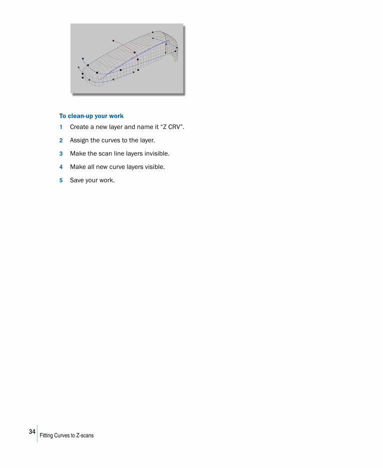
To clean-up your work
1 Create a new layer and name it “Z CRV”.
2 Assign the curves to the layer.
3 Make the scan line layers invisible.
4 Make all new curve layers visible.
5 Save your work.
34Fitting Curves to Z-scans
SURFACE CREATION
Learning Objectives
In this section you will learn how to:
● Understanding the theoretical line and helper surfaces.
Introduction to Patch Layouts
Fitting curves can be a time-consuming endeavour, and yet, even at this point in the tutorial your surface When edges do not have the same X, Y, and Z directions as the input data, additional curves are required to construct a proper surface. The new curves will need to be fitted and monitored for their deviation from the scan line. But instead of repeating the same tasks detailed in previous sections of the tutorial, you can take a break from fitting curves by learning about another method called Patch Layouts.
A Patch Layout is a master plan of the surfaces that cover the model. A Patch Layout shows which edges will need to be trimmed, how many surfaces in total will be required to complete the project, and how big they will need to be. For the beginner, most of the hard work happens before the point in the project where a Patch Layout can be generated. After generating the Patch Layout, you can concentrate on polishing and refinishing the surface to achieve a closer fit to the scan line. Once you become more familiar with structuring surface models, your workflow may change.
The subject of correct Patch Layout procedures is larger than the scope of this tutorial.
To learn more about Patch Layouts, examine surface data sets and experiment with taping surface edges onto physical models. These procedures will help you to think about the surface modeling process like a professional.
When approaching a new modeling assignment, try to imagine building the model by hand, or sketch ideas for how you would like to structure the surfaces. In situations where more complicated surfaces are required, such as ball corners, it may help to make small clay models by hand to rough out a tangible guide.
35
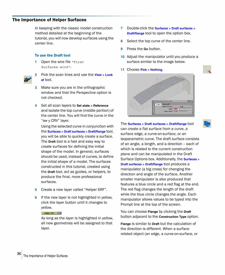
The Importance of Helper Surfaces
In keeping with the classic model construction method detailed at the beginning of the tutorial, you will now develop surfaces using the center line.
To use the Draft tool
1 Open the wire file "First Surfaces.wire".
2 Pick the scan lines and use the View > Look
at tool.
3 Make sure you are in the orthographic window and that the Perspective option is not checked.
4 Set all scan layers to Set state > Reference and isolate the top curve (middle portion) of the center line. You will find the curve in the “aw y CRV” layer.
Using the selected curve in conjunction with the Surfaces > Draft surfaces > Draft/flange tool, you will be able to quickly create a surface. The Draft tool is a fast and easy way to create surfaces for defining the initial shape of the model. In general, surfaces should be used, instead of curves, to define the initial shape of a model. The surfaces constructed in this tutorial, created using the Draft tool, act as guides, or helpers, to produce the final, more professional surfaces.
5 Create a new layer called “Helper SRF”.
6 If the new layer is not highlighted in yellow, click the layer button until it changes to yellow.
As long as the layer is highlighted in yellow, all new geometries will be assigned to that layer.
7 Double-click the Surfaces > Draft surfaces >
Draft/flange tool to open the option box.
8 Select the top curve of the center line.
9 Press the Go button.
10 Adjust the manipulator until you produce a surface similar to the image below.
11 Choose Pick > Nothing.
The Surfaces > Draft surfaces > Draft/flange tool can create a flat surface from a curve, a surface edge, a curve-on-surface, or an isoparametric curve. The draft surface consists of an angle, a length, and a direction – each of which is related to the current construction plane and can be manipulated in the Draft Surface Options box. Additionally, the Surfaces >
Draft surfaces > Draft/flange tool produces a manipulator (a big cross) for changing the direction and angle of the surface. Another smaller manipulator is also produced that features a blue circle and a red flag at the end. The red flag changes the length of the draft while the blue circle changes the angle. Each manipulator allows values to be typed into the Prompt line at the top of the screen.
You can choose Flange by clicking the Draft button adjacent to the Construction Type option.
Flange is similar to Draft but the calculation of the direction is different. When a surface related object (an edge, a curve-on-surface, or
36The Importance of Helper Surfaces
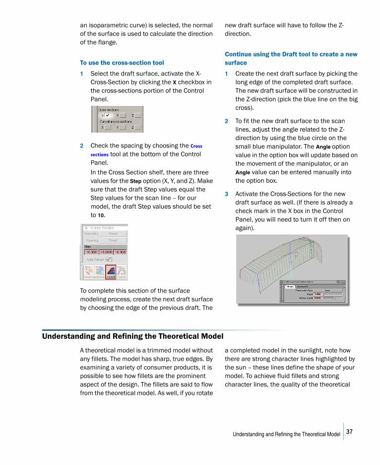
an isoparametric curve) is selected, the normal of the surface is used to calculate the direction of the flange.
To use the cross-section tool
1 Select the draft surface, activate the X-Cross-Section by clicking the X checkbox in the cross-sections portion of the Control Panel.
2 Check the spacing by choosing the Cross
sections tool at the bottom of the Control Panel.
In the Cross Section shelf, there are three values for the Step option (X, Y, and Z). Make sure that the draft Step values equal the Step values for the scan line – for our model, the draft Step values should be set to 10.
To complete this section of the surface modeling process, create the next draft surface by choosing the edge of the previous draft. The
new draft surface will have to follow the Z-direction.
Continue using the Draft tool to create a new surface
1 Create the next draft surface by picking the long edge of the completed draft surface. The new draft surface will be constructed in the Z-direction (pick the blue line on the big cross).
2 To fit the new draft surface to the scan lines, adjust the angle related to the Z-direction by using the blue circle on the small blue manipulator. The Angle option value in the option box will update based on the movement of the manipulator, or an Angle value can be entered manually into the option box.
3 Activate the Cross-Sections for the new draft surface as well. (If there is already a check mark in the X box in the Control Panel, you will need to turn it off then on again).
Understanding and Refining the Theoretical Model
A theoretical model is a trimmed model without any fillets. The model has sharp, true edges. By examining a variety of consumer products, it is possible to see how fillets are the prominent aspect of the design. The fillets are said to flow from the theoretical model. As well, if you rotate
a completed model in the sunlight, note how there are strong character lines highlighted by the sun – these lines define the shape of your model. To achieve fluid fillets and strong character lines, the quality of the theoretical
37Understanding and Refining the Theoretical Model

model must equal the expected quality of the finished model.
At this point in the tutorial, the model has a pointed theoretical line that was determined by creating the two draft surfaces. Examine the theoretical line and the two surfaces to see how closely they fit to the scan lines. To achieve a better result, try adjusting the length of the first draft surface and the angle of the second draft surface.
In regards to fitting the top surface, because the top surface is flat it will need to be shaped in order to fit to the scanned line. To shape the top surface, delete the construction history (draft), increase the flexibility (degree) of the surface, and direct model the surface.
To increase the degree of a surface
1 Choose Pick > Nothing.
2 Select the top surface.
3 In the Control Panel, turn on the CVs (Cv/
Hull).
4 In the Control Panel, increase the Degree value (in the V direction) from 1 to 2.
5 Press Enter.
6 You will be prompted to confirm that you really want to delete the history. Press YES to confirm.
7 Press the Accept button.
The top surface now has a Degree value of 2 in the V-direction and ensures the flexibility required to direct model the surface. To execute the direct model process, move the hulls and single CVs in such a manner that the green cross-section fits flush to the scan lines. At the same time, the second draft surface still has
history and will always update when changes are applied to the top surface. When modeling the top surface, remember to check for symmetry issues.
To direct model the surface
1 Choose the Object edit > Align > Symmetry
Plane Align tool.
2 Pick the top surface on the edge that meets the center line. A selection box will appear because SurfaceStudio detects the surface and the center line curve at the same time. Choose the surface.
You should see a collection of blue lines that highlight the surface as being symmetrical to the plane at the Y0 position. The Object edit > Align > Symmetry Plane Align
tool created history that will maintain the symmetry of the surfaces. If you move the CVs of the first two hulls in the Z-direction, the corresponding CVs will follow. Before using the tool, make certain that the Project
for Position option is activated in the Symmetry Plane Align tool’s option box.
3 Move the opposite hull down to achieve a better fit to the scan line.
4 Move the middle hull along the Y-direction to find a better fit.
5 To fit the second draft surface to the scan lines, choose single CVs and move them via the Move CV tool at the bottom of the Control Panel, with Mode set to SLIDE.
38Understanding and Refining the Theoretical Model
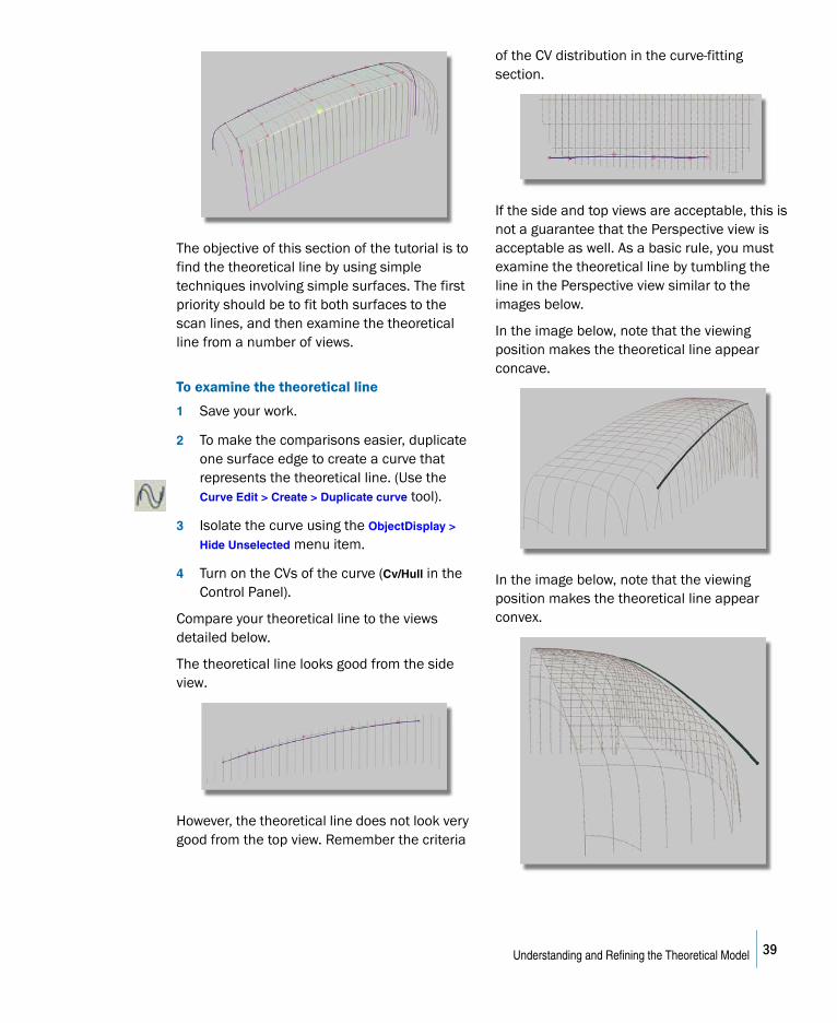
The objective of this section of the tutorial is to find the theoretical line by using simple techniques involving simple surfaces. The first priority should be to fit both surfaces to the scan lines, and then examine the theoretical line from a number of views.
To examine the theoretical line
1 Save your work.
2 To make the comparisons easier, duplicate one surface edge to create a curve that represents the theoretical line. (Use the Curve Edit > Create > Duplicate curve tool).
3 Isolate the curve using the ObjectDisplay >
Hide Unselected menu item.
4 Turn on the CVs of the curve (Cv/Hull in the Control Panel).
Compare your theoretical line to the views detailed below.
The theoretical line looks good from the side view.
However, the theoretical line does not look very good from the top view. Remember the criteria
of the CV distribution in the curve-fitting section.
If the side and top views are acceptable, this is not a guarantee that the Perspective view is acceptable as well. As a basic rule, you must examine the theoretical line by tumbling the line in the Perspective view similar to the images below.
In the image below, note that the viewing position makes the theoretical line appear concave.
In the image below, note that the viewing position makes the theoretical line appear convex.
39Understanding and Refining the Theoretical Model
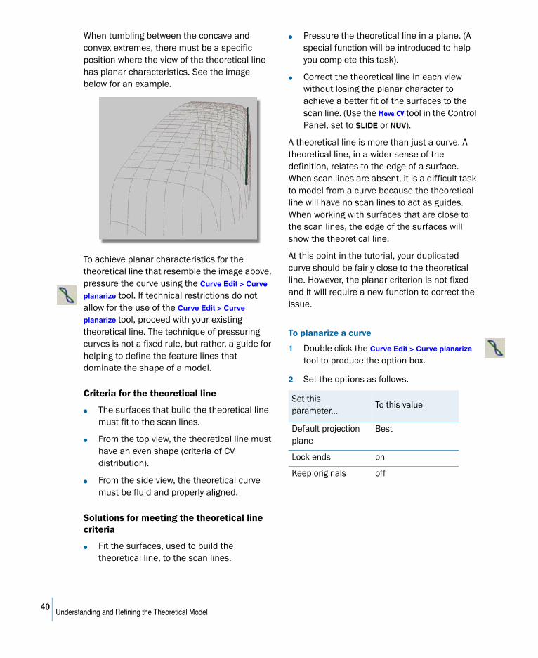
When tumbling between the concave and convex extremes, there must be a specific position where the view of the theoretical line has planar characteristics. See the image below for an example.
To achieve planar characteristics for the theoretical line that resemble the image above, pressure the curve using the Curve Edit > Curve
planarize tool. If technical restrictions do not allow for the use of the Curve Edit > Curve
planarize tool, proceed with your existing theoretical line. The technique of pressuring curves is not a fixed rule, but rather, a guide for helping to define the feature lines that dominate the shape of a model.
Criteria for the theoretical line
● The surfaces that build the theoretical line must fit to the scan lines.
● From the top view, the theoretical line must have an even shape (criteria of CV distribution).
● From the side view, the theoretical curve must be fluid and properly aligned.
Solutions for meeting the theoretical line criteria
● Fit the surfaces, used to build the theoretical line, to the scan lines.
● Pressure the theoretical line in a plane. (A special function will be introduced to help you complete this task).
● Correct the theoretical line in each view without losing the planar character to achieve a better fit of the surfaces to the scan line. (Use the Move CV tool in the Control Panel, set to SLIDE or NUV).
A theoretical line is more than just a curve. A theoretical line, in a wider sense of the definition, relates to the edge of a surface. When scan lines are absent, it is a difficult task to model from a curve because the theoretical line will have no scan lines to act as guides. When working with surfaces that are close to the scan lines, the edge of the surfaces will show the theoretical line.
At this point in the tutorial, your duplicated curve should be fairly close to the theoretical line. However, the planar criterion is not fixed and it will require a new function to correct the issue.
To planarize a curve
1 Double-click the Curve Edit > Curve planarize tool to produce the option box.
2 Set the options as follows.
Set this parameter...
To this value
Default projection plane
Best
Lock ends on
Keep originals off
40Understanding and Refining the Theoretical Model
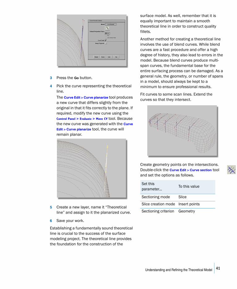
3 Press the Go button.
4 Pick the curve representing the theoretical line.
The Curve Edit > Curve planarize tool produces a new curve that differs slightly from the original in that it fits correctly to the plane. If required, modify the new curve using the Control Panel > Evaluate > Move CV tool. Because the new curve was generated with the Curve
Edit > Curve planarize tool, the curve will remain planar.
5 Create a new layer, name it “Theoretical line” and assign to it the planarized curve.
6 Save your work.
Establishing a fundamentally sound theoretical line is crucial to the success of the surface modeling project. The theoretical line provides the foundation for the construction of the
surface model. As well, remember that it is equally important to maintain a smooth theoretical line in order to construct quality fillets.
Another method for creating a theoretical line involves the use of blend curves. While blend curves are a fast procedure and offer a high degree of history, they also lead to errors in the model. Because blend curves produce multi-span curves, the fundamental base for the entire surfacing process can be damaged. As a general rule, the geometry, or number of spans in a model, should always be kept to a minimum to ensure professional results.
Fit curves to some scan lines. Extend the curves so that they intersect.
Create geometry points on the intersections. Double-click the Curve Edit > Curve section tool and set the options as follows.
Set this parameter...
To this value
Sectioning mode Slice
Slice creation mode Insert points
Sectioning criterion Geometry
41Understanding and Refining the Theoretical Model
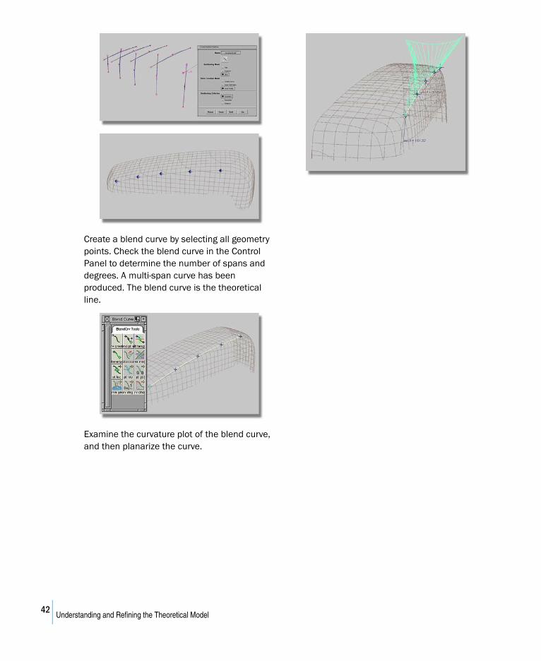
Create a blend curve by selecting all geometry points. Check the blend curve in the Control Panel to determine the number of spans and degrees. A multi-span curve has been produced. The blend curve is the theoretical line.
Examine the curvature plot of the blend curve, and then planarize the curve.
42Understanding and Refining the Theoretical Model

Summary
● Check your model before beginning the fillets. The edges of the trimmed model must be clean as it is not possible to correct a model using the various options in the Surfaces > Surface fillet tool option box.
● Many curves that define feature lines are planar in a special view. Once you have achieved an acceptable shape, planarize the curve to refine the shape.
● When modifying planar curves, the planar characteristics must be maintained. Use the SLIDE or NUV options in the Control Panel >
Evaluate > Move CV tool. The NUV option works on curves, but does not maintain planar characteristics on surface edges.
43Understanding and Refining the Theoretical Model

44Understanding and Refining the Theoretical Model
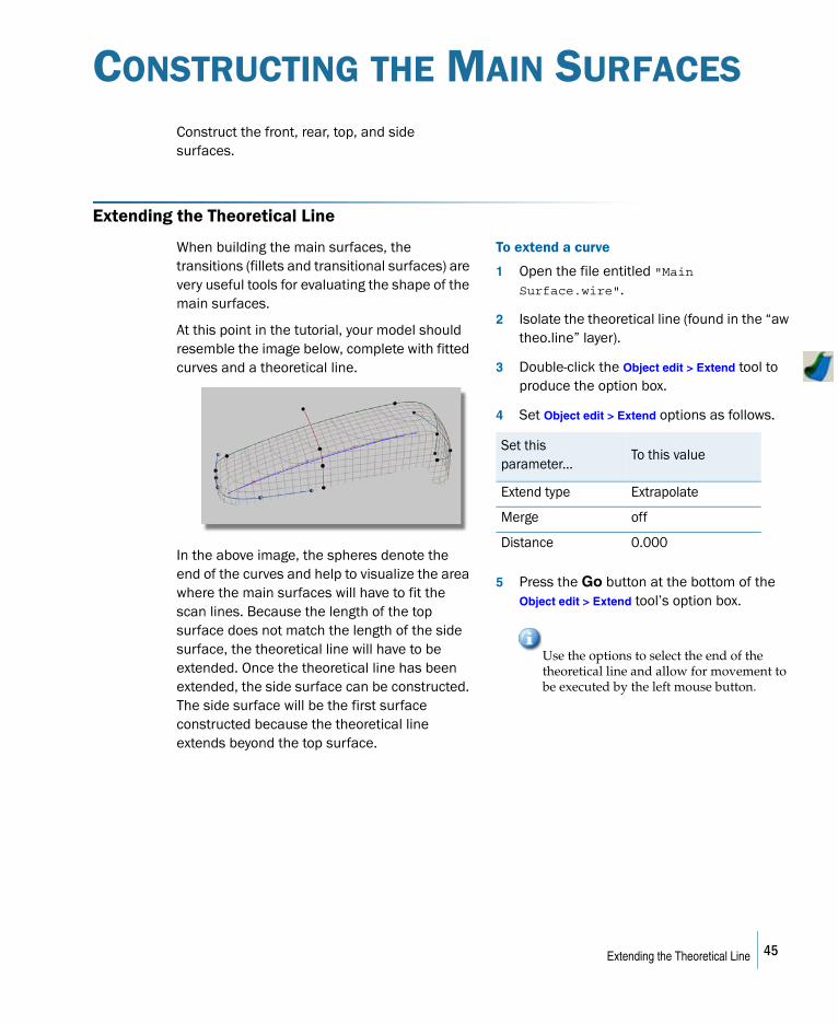
CONSTRUCTING THE MAIN SURFACES
Construct the front, rear, top, and side surfaces.
Extending the Theoretical Line
When building the main surfaces, the transitions (fillets and transitional surfaces) are very useful tools for evaluating the shape of the main surfaces.
At this point in the tutorial, your model should resemble the image below, complete with fitted curves and a theoretical line.
In the above image, the spheres denote the end of the curves and help to visualize the area where the main surfaces will have to fit the scan lines. Because the length of the top surface does not match the length of the side surface, the theoretical line will have to be extended. Once the theoretical line has been extended, the side surface can be constructed. The side surface will be the first surface constructed because the theoretical line extends beyond the top surface.
To extend a curve
1 Open the file entitled "Main Surface.wire".
2 Isolate the theoretical line (found in the “aw theo.line” layer).
3 Double-click the Object edit > Extend tool to produce the option box.
4 Set Object edit > Extend options as follows.
5 Press the Go button at the bottom of the Object edit > Extend tool’s option box.
Use the options to select the end of the theoretical line and allow for movement to be executed by the left mouse button.
Set this parameter...
To this value
Extend type Extrapolate
Merge off
Distance 0.000
45Extending the Theoretical Line
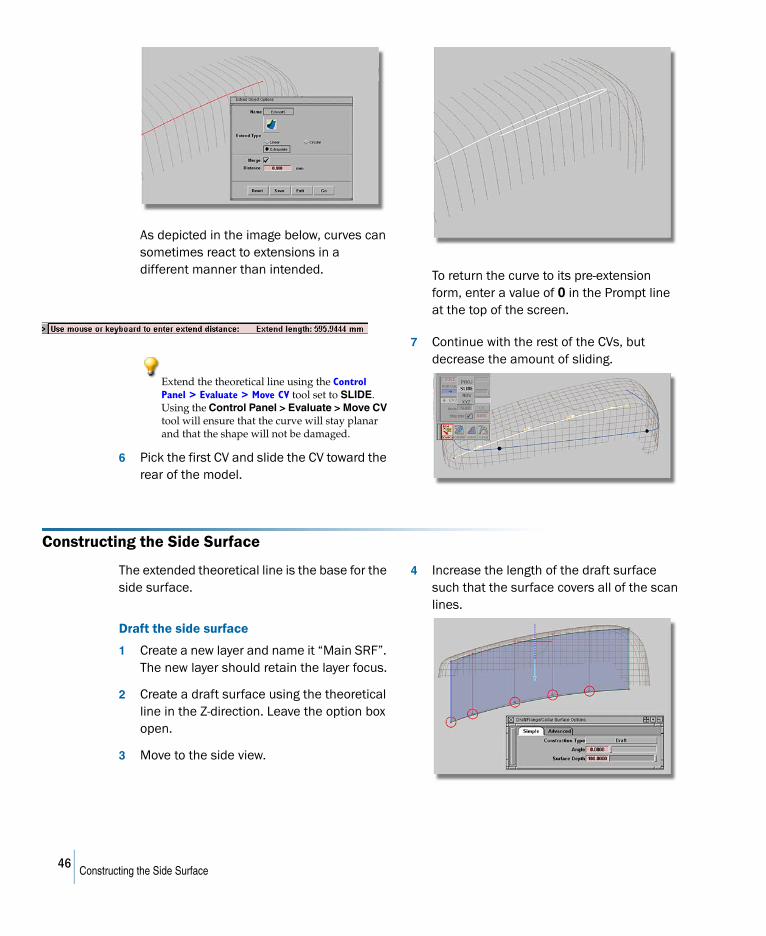
As depicted in the image below, curves can sometimes react to extensions in a different manner than intended. To return the curve to its pre-extension
form, enter a value of 0 in the Prompt line at the top of the screen.
Extend the theoretical line using the Control Panel > Evaluate > Move CV tool set to SLIDE. Using the Control Panel > Evaluate > Move CV tool will ensure that the curve will stay planar and that the shape will not be damaged.
6 Pick the first CV and slide the CV toward the rear of the model.
7 Continue with the rest of the CVs, but decrease the amount of sliding.
Constructing the Side Surface
The extended theoretical line is the base for the side surface.
Draft the side surface
1 Create a new layer and name it “Main SRF”. The new layer should retain the layer focus.
2 Create a draft surface using the theoretical line in the Z-direction. Leave the option box open.
3 Move to the side view.
4 Increase the length of the draft surface such that the surface covers all of the scan lines.
46Constructing the Side Surface
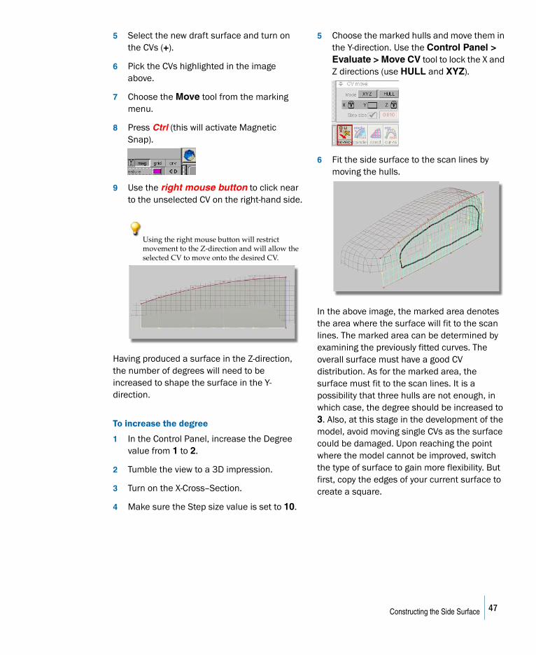
5 Select the new draft surface and turn on the CVs (+).
6 Pick the CVs highlighted in the image above.
7 Choose the Move tool from the marking menu.
8 Press Ctrl (this will activate Magnetic Snap).
9 Use the right mouse button to click near to the unselected CV on the right-hand side.
Using the right mouse button will restrict movement to the Z-direction and will allow the selected CV to move onto the desired CV.
Having produced a surface in the Z-direction, the number of degrees will need to be increased to shape the surface in the Y-direction.
To increase the degree
1 In the Control Panel, increase the Degree value from 1 to 2.
2 Tumble the view to a 3D impression.
3 Turn on the X-Cross–Section.
4 Make sure the Step size value is set to 10.
5 Choose the marked hulls and move them in the Y-direction. Use the Control Panel > Evaluate > Move CV tool to lock the X and Z directions (use HULL and XYZ).
6 Fit the side surface to the scan lines by moving the hulls.
In the above image, the marked area denotes the area where the surface will fit to the scan lines. The marked area can be determined by examining the previously fitted curves. The overall surface must have a good CV distribution. As for the marked area, the surface must fit to the scan lines. It is a possibility that three hulls are not enough, in which case, the degree should be increased to 3. Also, at this stage in the development of the model, avoid moving single CVs as the surface could be damaged. Upon reaching the point where the model cannot be improved, switch the type of surface to gain more flexibility. But first, copy the edges of your current surface to create a square.
47Constructing the Side Surface
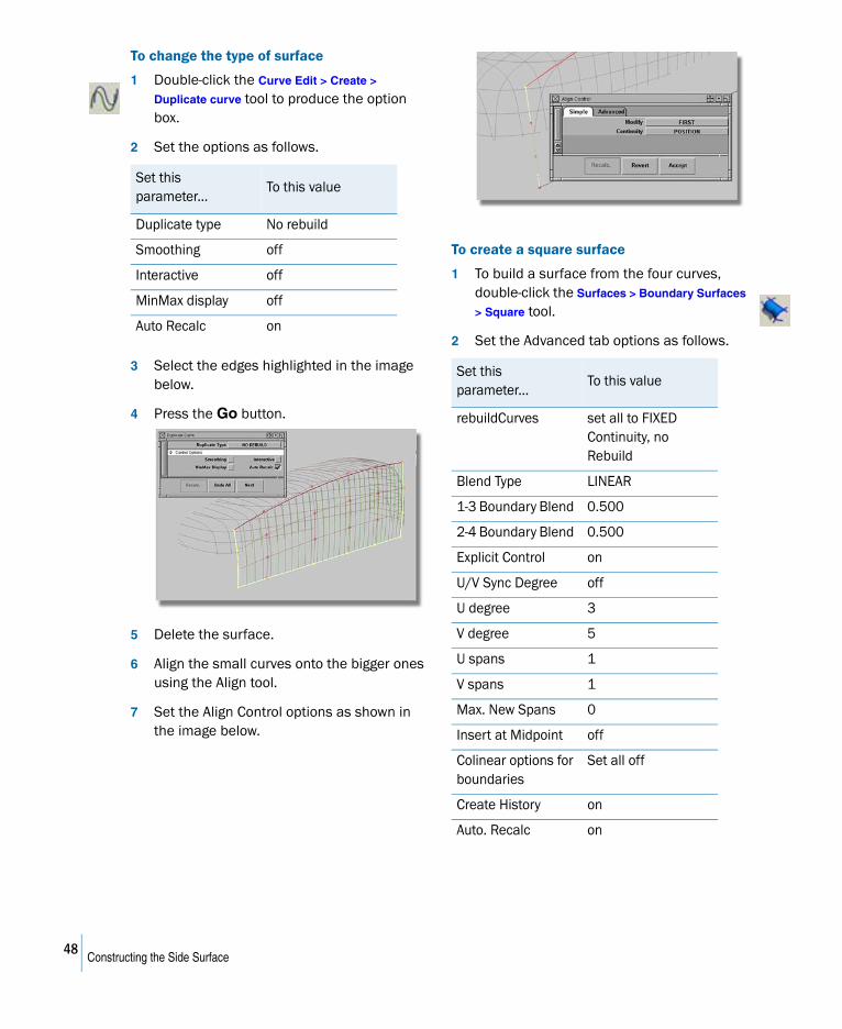
To change the type of surface
1 Double-click the Curve Edit > Create >
Duplicate curve tool to produce the option box.
2 Set the options as follows.
3 Select the edges highlighted in the image below.
4 Press the Go button.
5 Delete the surface.
6 Align the small curves onto the bigger ones using the Align tool.
7 Set the Align Control options as shown in the image below.
To create a square surface
1 To build a surface from the four curves, double-click the Surfaces > Boundary Surfaces
> Square tool.
2 Set the Advanced tab options as follows.
Set this parameter...
To this value
Duplicate type No rebuild
Smoothing off
Interactive off
MinMax display off
Auto Recalc on
Set this parameter...
To this value
rebuildCurves set all to FIXED Continuity, no Rebuild
Blend Type LINEAR
1-3 Boundary Blend 0.500
2-4 Boundary Blend 0.500
Explicit Control on
U/V Sync Degree off
U degree 3
V degree 5
U spans 1
V spans 1
Max. New Spans 0
Insert at Midpoint off
Colinear options for boundaries
Set all off
Create History on
Auto. Recalc on
48Constructing the Side Surface
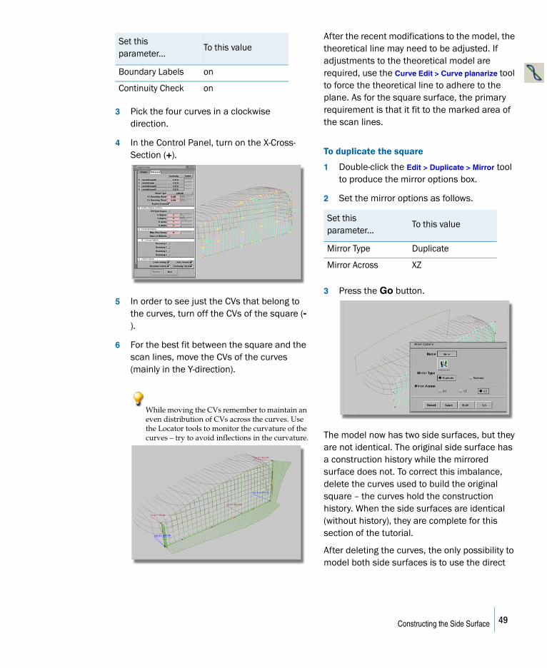
3 Pick the four curves in a clockwise direction.
4 In the Control Panel, turn on the X-Cross-Section (+).
5 In order to see just the CVs that belong to the curves, turn off the CVs of the square (-).
6 For the best fit between the square and the scan lines, move the CVs of the curves (mainly in the Y-direction).
While moving the CVs remember to maintain an even distribution of CVs across the curves. Use the Locator tools to monitor the curvature of the curves – try to avoid inflections in the curvature.
After the recent modifications to the model, the theoretical line may need to be adjusted. If adjustments to the theoretical model are required, use the Curve Edit > Curve planarize tool to force the theoretical line to adhere to the plane. As for the square surface, the primary requirement is that it fit to the marked area of the scan lines.
To duplicate the square
1 Double-click the Edit > Duplicate > Mirror tool to produce the mirror options box.
2 Set the mirror options as follows.
3 Press the Go button.
The model now has two side surfaces, but they are not identical. The original side surface has a construction history while the mirrored surface does not. To correct this imbalance, delete the curves used to build the original square – the curves hold the construction history. When the side surfaces are identical (without history), they are complete for this section of the tutorial.
After deleting the curves, the only possibility to model both side surfaces is to use the direct
Boundary Labels on
Continuity Check on
Set this parameter...
To this value
Set this parameter...
To this value
Mirror Type Duplicate
Mirror Across XZ
49Constructing the Side Surface
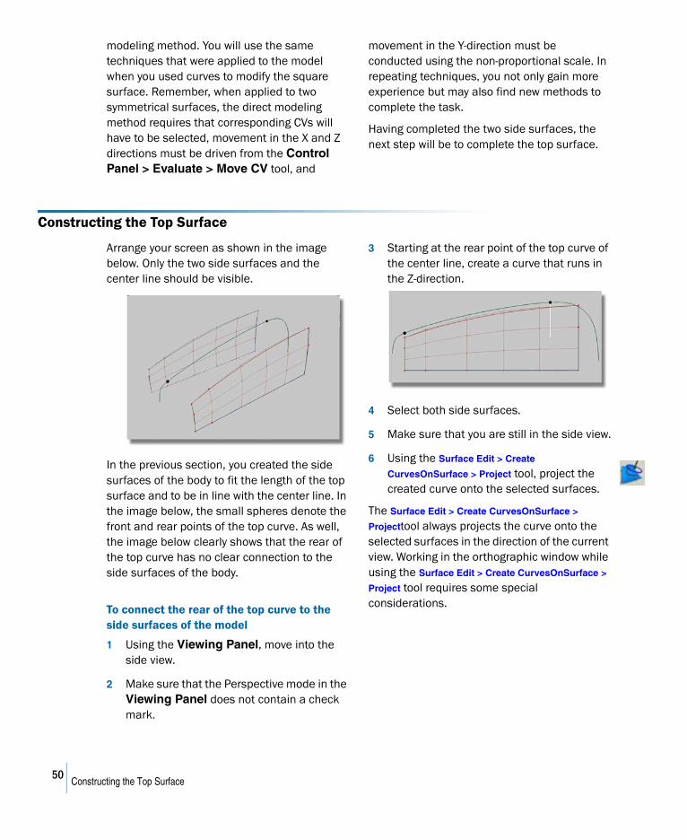
modeling method. You will use the same techniques that were applied to the model when you used curves to modify the square surface. Remember, when applied to two symmetrical surfaces, the direct modeling method requires that corresponding CVs will have to be selected, movement in the X and Z directions must be driven from the Control Panel > Evaluate > Move CV tool, and
movement in the Y-direction must be conducted using the non-proportional scale. In repeating techniques, you not only gain more experience but may also find new methods to complete the task.
Having completed the two side surfaces, the next step will be to complete the top surface.
Constructing the Top Surface
Arrange your screen as shown in the image below. Only the two side surfaces and the center line should be visible.
In the previous section, you created the side surfaces of the body to fit the length of the top surface and to be in line with the center line. In the image below, the small spheres denote the front and rear points of the top curve. As well, the image below clearly shows that the rear of the top curve has no clear connection to the side surfaces of the body.
To connect the rear of the top curve to the side surfaces of the model
1 Using the Viewing Panel, move into the side view.
2 Make sure that the Perspective mode in the Viewing Panel does not contain a check mark.
3 Starting at the rear point of the top curve of the center line, create a curve that runs in the Z-direction.
4 Select both side surfaces.
5 Make sure that you are still in the side view.
6 Using the Surface Edit > Create
CurvesOnSurface > Project tool, project the created curve onto the selected surfaces.
The Surface Edit > Create CurvesOnSurface >
Projecttool always projects the curve onto the selected surfaces in the direction of the current view. Working in the orthographic window while using the Surface Edit > Create CurvesOnSurface >
Project tool requires some special considerations.
50Constructing the Top Surface
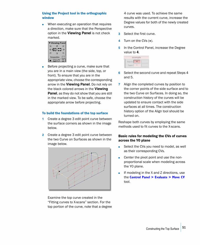
Using the Project tool in the orthographic window
● When executing an operation that requires a direction, make sure that the Perspective option in the Viewing Panel is not check marked.
● Before projecting a curve, make sure that you are in a main view (the side, top, or front). To ensure that you are in the appropriate view, choose the corresponding arrow in the Viewing Panel. Do not rely on the black colored arrows in the Viewing Panel, as they do not show that you are still in the marked view. To be safe, choose the appropriate arrow before projecting.
To build the foundations of the top surface
1 Create a degree 3 edit point curve between the surface corners as shown in the image below.
2 Create a degree 3 edit point curve between the two Curve on Surfaces as shown in the image below.
Examine the top curve created in the “Fitting curves to X-scans” section. For the top portion of the curve, note that a degree
4 curve was used. To achieve the same results with the current curve, increase the Degree values for both of the newly created curves.
3 Select the first curve.
4 Turn on the CVs (+).
5 In the Control Panel, increase the Degree value to 4.
6 Select the second curve and repeat Steps 4 and 5.
7 Align the completed curves by position to the corner points of the side surface and to the two Curve on Surfaces. In doing so, the construction history of the curves will be updated to ensure contact with the side surfaces at all times. The construction history option of the Align tool should be turned on.
Reshape both curves by employing the same methods used to fit curves to the X-scans.
Basic rules for modeling the CVs of curves across the Y0 plane
● Select the CVs you need to model, as well as their corresponding CVs.
● Center the pivot point and use the non-proportional scale when modeling across the Y0 plane.
● If modeling in the X and Z directions, use the Control Panel > Evaluate > Move CV tool.
51Constructing the Top Surface
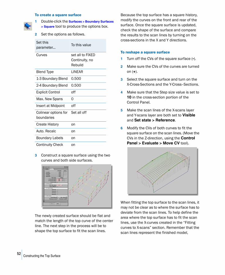
To create a square surface
1 Double-click the Surfaces > Boundary Surfaces
> Square tool to produce the options box.
2 Set the options as follows.
3 Construct a square surface using the two curves and both side surfaces.
The newly created surface should be flat and match the length of the top curve of the center line. The next step in the process will be to shape the top surface to fit the scan lines.
Because the top surface has a square history, modify the curves on the front and rear of the surface. Once the square surface is updated, check the shape of the surface and compare the results to the scan lines by turning on the cross-sections in the X and Y directions.
To reshape a square surface
1 Turn off the CVs of the square surface (-).
2 Make sure the CVs of the curves are turned on (+).
3 Select the square surface and turn on the X-Cross-Sections and the Y-Cross–Sections.
4 Make sure that the Step size value is set to 10 in the cross-section portion of the Control Panel.
5 Make the scan lines of the X-scans layer and Y-scans layer are both set to Visible and Set state > Reference.
6 Modify the CVs of both curves to fit the square surface on the scan lines. (Move the CVs in the Z-direction, using the Control Panel > Evaluate > Move CV tool).
When fitting the top surface to the scan lines, it may not be clear as to where the surface has to deviate from the scan lines. To help define the area where the top surface has to fit the scan lines, use the X-curves created in the “Fitting curves to X-scans” section. Remember that the scan lines represent the finished model,
Set this parameter...
To this value
Curves set all to FIXED Continuity, no Rebuild
Blend Type LINEAR
1-3 Boundary Blend 0.500
2-4 Boundary Blend 0.500
Explicit Control off
Max. New Spans 0
Insert at Midpoint off
Colinear options for boundaries
Set all off
Create History on
Auto. Recalc on
Boundary Labels on
Continuity Check on
52Constructing the Top Surface
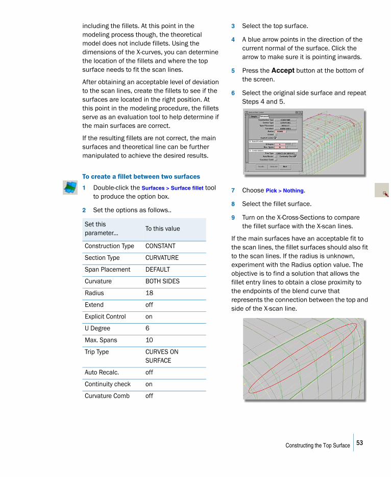
including the fillets. At this point in the modeling process though, the theoretical model does not include fillets. Using the dimensions of the X-curves, you can determine the location of the fillets and where the top surface needs to fit the scan lines.
After obtaining an acceptable level of deviation to the scan lines, create the fillets to see if the surfaces are located in the right position. At this point in the modeling procedure, the fillets serve as an evaluation tool to help determine if the main surfaces are correct.
If the resulting fillets are not correct, the main surfaces and theoretical line can be further manipulated to achieve the desired results.
To create a fillet between two surfaces
1 Double-click the Surfaces > Surface fillet tool to produce the option box.
2 Set the options as follows..
3 Select the top surface.
4 A blue arrow points in the direction of the current normal of the surface. Click the arrow to make sure it is pointing inwards.
5 Press the Accept button at the bottom of the screen.
6 Select the original side surface and repeat Steps 4 and 5.
7 Choose Pick > Nothing.
8 Select the fillet surface.
9 Turn on the X-Cross-Sections to compare the fillet surface with the X-scan lines.
If the main surfaces have an acceptable fit to the scan lines, the fillet surfaces should also fit to the scan lines. If the radius is unknown, experiment with the Radius option value. The objective is to find a solution that allows the fillet entry lines to obtain a close proximity to the endpoints of the blend curve that represents the connection between the top and side of the X-scan line.
Set this parameter...
To this value
Construction Type CONSTANT
Section Type CURVATURE
Span Placement DEFAULT
Curvature BOTH SIDES
Radius 18
Extend off
Explicit Control on
U Degree 6
Max. Spans 10
Trip Type CURVES ON SURFACE
Auto Recalc. off
Continuity check on
Curvature Comb off
53Constructing the Top Surface
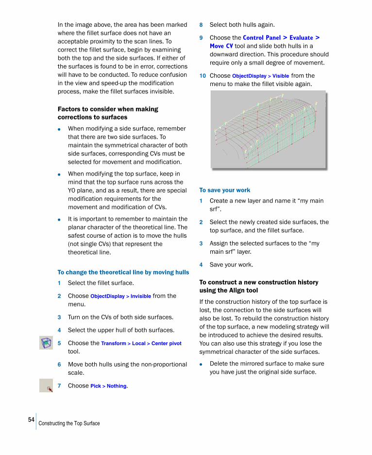
In the image above, the area has been marked where the fillet surface does not have an acceptable proximity to the scan lines. To correct the fillet surface, begin by examining both the top and the side surfaces. If either of the surfaces is found to be in error, corrections will have to be conducted. To reduce confusion in the view and speed-up the modification process, make the fillet surfaces invisible.
Factors to consider when making corrections to surfaces
● When modifying a side surface, remember that there are two side surfaces. To maintain the symmetrical character of both side surfaces, corresponding CVs must be selected for movement and modification.
● When modifying the top surface, keep in mind that the top surface runs across the Y0 plane, and as a result, there are special modification requirements for the movement and modification of CVs.
● It is important to remember to maintain the planar character of the theoretical line. The safest course of action is to move the hulls (not single CVs) that represent the theoretical line.
To change the theoretical line by moving hulls
1 Select the fillet surface.
2 Choose ObjectDisplay > Invisible from the menu.
3 Turn on the CVs of both side surfaces.
4 Select the upper hull of both surfaces.
5 Choose the Transform > Local > Center pivot tool.
6 Move both hulls using the non-proportional scale.
7 Choose Pick > Nothing.
8 Select both hulls again.
9 Choose the Control Panel > Evaluate > Move CV tool and slide both hulls in a downward direction. This procedure should require only a small degree of movement.
10 Choose ObjectDisplay > Visible from the menu to make the fillet visible again.
To save your work
1 Create a new layer and name it “my main srf”.
2 Select the newly created side surfaces, the top surface, and the fillet surface.
3 Assign the selected surfaces to the “my main srf” layer.
4 Save your work.
To construct a new construction history using the Align tool
If the construction history of the top surface is lost, the connection to the side surfaces will also be lost. To rebuild the construction history of the top surface, a new modeling strategy will be introduced to achieve the desired results. You can also use this strategy if you lose the symmetrical character of the side surfaces.
● Delete the mirrored surface to make sure you have just the original side surface.
54Constructing the Top Surface
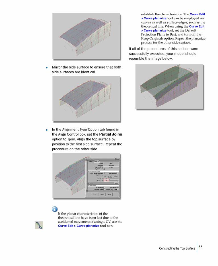
● Mirror the side surface to ensure that both side surfaces are identical.
● In the Alignment Type Option tab found in the Align Control box, set the Partial Joins option to Tjoin. Align the top surface by position to the first side surface. Repeat the procedure on the other side.
If the planar characteristics of the theoretical line have been lost due to the accidental movement of a single CV, use the Curve Edit > Curve planarize tool to re-
establish the characteristics. The Curve Edit > Curve planarize tool can be employed on curves as well as surface edges, such as the theoretical line. When using the Curve Edit > Curve planarize tool, set the Default Projection Plane to Best, and turn off the Keep Originals option. Repeat the planarize process for the other side surface.
If all of the procedures of this section were successfully executed, your model should resemble the image below.
55Constructing the Top Surface
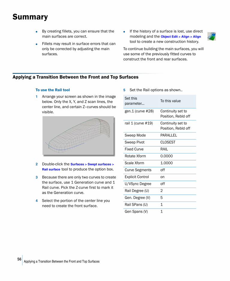
Summary
● By creating fillets, you can ensure that the main surfaces are correct.
● Fillets may result in surface errors that can only be corrected by adjusting the main surfaces.
● If the history of a surface is lost, use direct modeling and the Object Edit > Align > Align tool to create a new construction history.
To continue building the main surfaces, you will use some of the previously fitted curves to construct the front and rear surfaces.
Applying a Transition Between the Front and Top Surfaces
To use the Rail tool
1 Arrange your screen as shown in the image below. Only the X, Y, and Z scan lines, the center line, and certain Z–curves should be visible.
2 Double-click the Surfaces > Swept surfaces >
Rail surface tool to produce the option box.
3 Because there are only two curves to create the surface, use 1 Generation curve and 1 Rail curve. Pick the Z-curve first to mark it as the Generation curve.
4 Select the portion of the center line you need to create the front surface.
5 Set the Rail options as shown..
Set this parameter...
To this value
gen.1 (curve #28) Continuity set to Position, Rebld off
rail 1 (curve #19) Continuity set to Position, Rebld off
Sweep Mode PARALLEL
Sweep Pivot CLOSEST
Fixed Curve RAIL
Rotate Xform 0.0000
Scale Xform 1.0000
Curve Segments off
Explicit Control on
U/VSync Degree off
Rail Degree (U) 2
Gen. Degree (V) 5
Rail SPans (U) 1
Gen Spans (V) 1
56Applying a Transition Between the Front and Top Surfaces
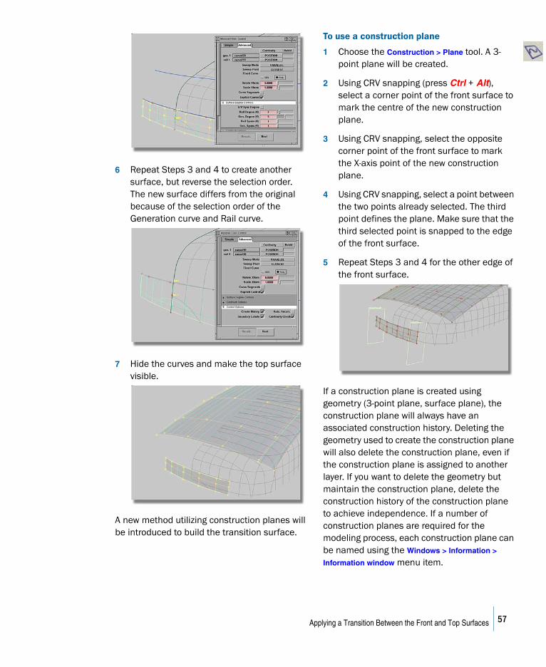
6 Repeat Steps 3 and 4 to create another surface, but reverse the selection order. The new surface differs from the original because of the selection order of the Generation curve and Rail curve.
7 Hide the curves and make the top surface visible.
A new method utilizing construction planes will be introduced to build the transition surface.
To use a construction plane
1 Choose the Construction > Plane tool. A 3-point plane will be created.
2 Using CRV snapping (press Ctrl + Alt), select a corner point of the front surface to mark the centre of the new construction plane.
3 Using CRV snapping, select the opposite corner point of the front surface to mark the X-axis point of the new construction plane.
4 Using CRV snapping, select a point between the two points already selected. The third point defines the plane. Make sure that the third selected point is snapped to the edge of the front surface.
5 Repeat Steps 3 and 4 for the other edge of the front surface.
If a construction plane is created using geometry (3-point plane, surface plane), the construction plane will always have an associated construction history. Deleting the geometry used to create the construction plane will also delete the construction plane, even if the construction plane is assigned to another layer. If you want to delete the geometry but maintain the construction plane, delete the construction history of the construction plane to achieve independence. If a number of construction planes are required for the modeling process, each construction plane can be named using the Windows > Information >
Information window menu item.
57Applying a Transition Between the Front and Top Surfaces
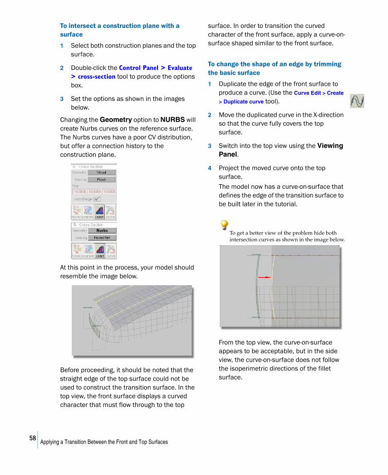
To intersect a construction plane with a surface
1 Select both construction planes and the top surface.
2 Double-click the Control Panel > Evaluate > cross-section tool to produce the options box.
3 Set the options as shown in the images below.
Changing the Geometry option to NURBS will create Nurbs curves on the reference surface. The Nurbs curves have a poor CV distribution, but offer a connection history to the construction plane.
At this point in the process, your model should resemble the image below.
Before proceeding, it should be noted that the straight edge of the top surface could not be used to construct the transition surface. In the top view, the front surface displays a curved character that must flow through to the top
surface. In order to transition the curved character of the front surface, apply a curve-on-surface shaped similar to the front surface.
To change the shape of an edge by trimming the basic surface
1 Duplicate the edge of the front surface to produce a curve. (Use the Curve Edit > Create
> Duplicate curve tool).
2 Move the duplicated curve in the X-direction so that the curve fully covers the top surface.
3 Switch into the top view using the Viewing Panel.
4 Project the moved curve onto the top surface.
The model now has a curve-on-surface that defines the edge of the transition surface to be built later in the tutorial.
To get a better view of the problem hide both intersection curves as shown in the image below.
From the top view, the curve-on-surface appears to be acceptable, but in the side view, the curve-on-surface does not follow the isoperimetric directions of the fillet surface.
58Applying a Transition Between the Front and Top Surfaces
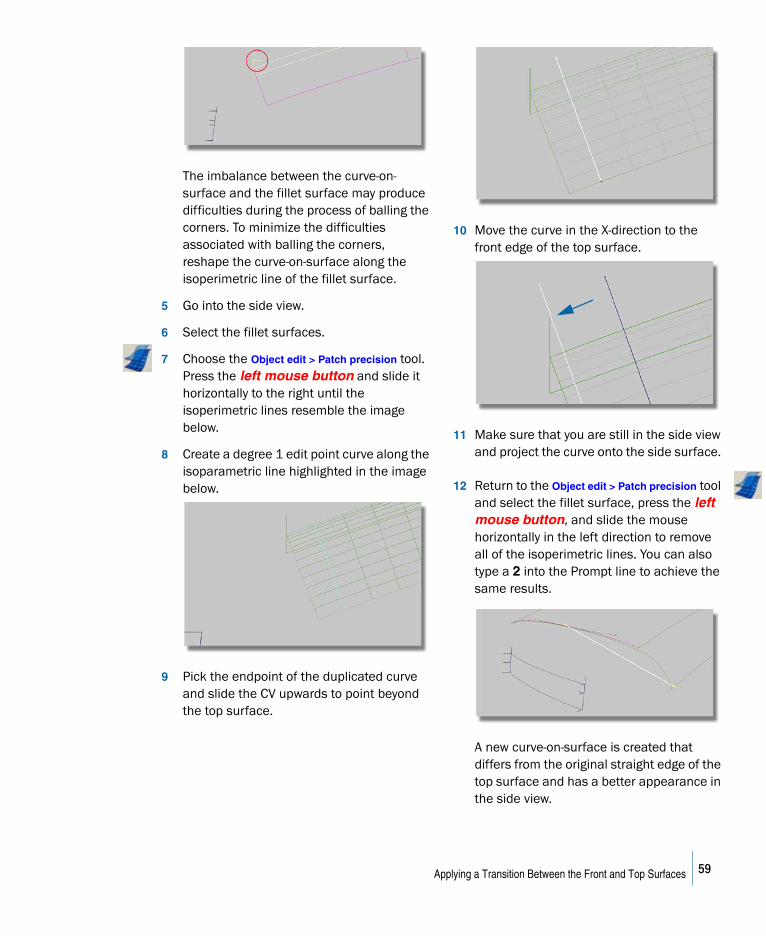
The imbalance between the curve-on-surface and the fillet surface may produce difficulties during the process of balling the corners. To minimize the difficulties associated with balling the corners, reshape the curve-on-surface along the isoperimetric line of the fillet surface.
5 Go into the side view.
6 Select the fillet surfaces.
7 Choose the Object edit > Patch precision tool. Press the left mouse button and slide it horizontally to the right until the isoperimetric lines resemble the image below.
8 Create a degree 1 edit point curve along the isoparametric line highlighted in the image below.
9 Pick the endpoint of the duplicated curve and slide the CV upwards to point beyond the top surface.
10 Move the curve in the X-direction to the front edge of the top surface.
11 Make sure that you are still in the side view and project the curve onto the side surface.
12 Return to the Object edit > Patch precision tool and select the fillet surface, press the left mouse button, and slide the mouse horizontally in the left direction to remove all of the isoperimetric lines. You can also type a 2 into the Prompt line to achieve the same results.
A new curve-on-surface is created that differs from the original straight edge of the top surface and has a better appearance in the side view.
59Applying a Transition Between the Front and Top Surfaces
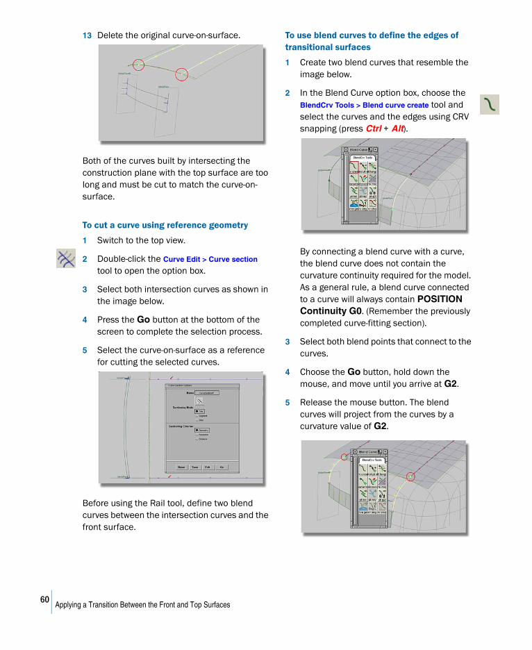
13 Delete the original curve-on-surface.
Both of the curves built by intersecting the construction plane with the top surface are too long and must be cut to match the curve-on-surface.
To cut a curve using reference geometry
1 Switch to the top view.
2 Double-click the Curve Edit > Curve section tool to open the option box.
3 Select both intersection curves as shown in the image below.
4 Press the Go button at the bottom of the screen to complete the selection process.
5 Select the curve-on-surface as a reference for cutting the selected curves.
Before using the Rail tool, define two blend curves between the intersection curves and the front surface.
To use blend curves to define the edges of transitional surfaces
1 Create two blend curves that resemble the image below.
2 In the Blend Curve option box, choose the BlendCrv Tools > Blend curve create tool and select the curves and the edges using CRV snapping (press Ctrl + Alt).
By connecting a blend curve with a curve, the blend curve does not contain the curvature continuity required for the model. As a general rule, a blend curve connected to a curve will always contain POSITION Continuity G0. (Remember the previously completed curve-fitting section).
3 Select both blend points that connect to the curves.
4 Choose the Go button, hold down the mouse, and move until you arrive at G2.
5 Release the mouse button. The blend curves will project from the curves by a curvature value of G2.
60Applying a Transition Between the Front and Top Surfaces
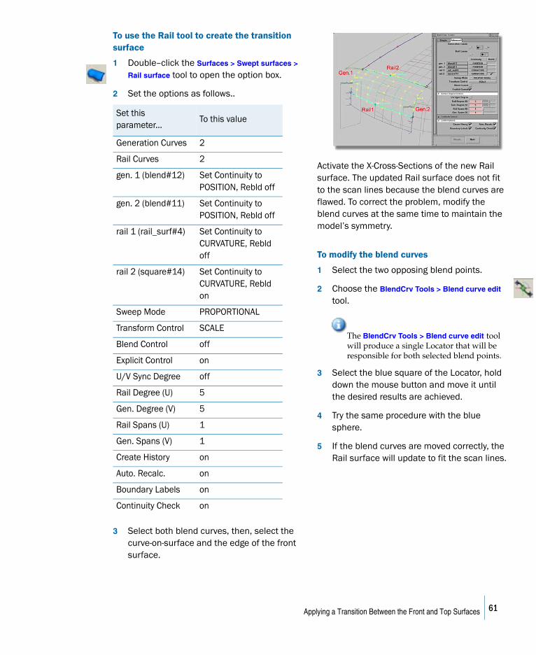
To use the Rail tool to create the transition surface
1 Double–click the Surfaces > Swept surfaces >
Rail surface tool to open the option box.
2 Set the options as follows..
3 Select both blend curves, then, select the curve-on-surface and the edge of the front surface.
Activate the X-Cross-Sections of the new Rail surface. The updated Rail surface does not fit to the scan lines because the blend curves are flawed. To correct the problem, modify the blend curves at the same time to maintain the model’s symmetry.
To modify the blend curves
1 Select the two opposing blend points.
2 Choose the BlendCrv Tools > Blend curve edit tool.
The BlendCrv Tools > Blend curve edit tool will produce a single Locator that will be responsible for both selected blend points.
3 Select the blue square of the Locator, hold down the mouse button and move it until the desired results are achieved.
4 Try the same procedure with the blue sphere.
5 If the blend curves are moved correctly, the Rail surface will update to fit the scan lines.
Set this parameter...
To this value
Generation Curves 2
Rail Curves 2
gen. 1 (blend#12) Set Continuity to POSITION, Rebld off
gen. 2 (blend#11) Set Continuity to POSITION, Rebld off
rail 1 (rail_surf#4) Set Continuity to CURVATURE, Rebld off
rail 2 (square#14) Set Continuity to CURVATURE, Rebld on
Sweep Mode PROPORTIONAL
Transform Control SCALE
Blend Control off
Explicit Control on
U/V Sync Degree off
Rail Degree (U) 5
Gen. Degree (V) 5
Rail Spans (U) 1
Gen. Spans (V) 1
Create History on
Auto. Recalc. on
Boundary Labels on
Continuity Check on
61Applying a Transition Between the Front and Top Surfaces
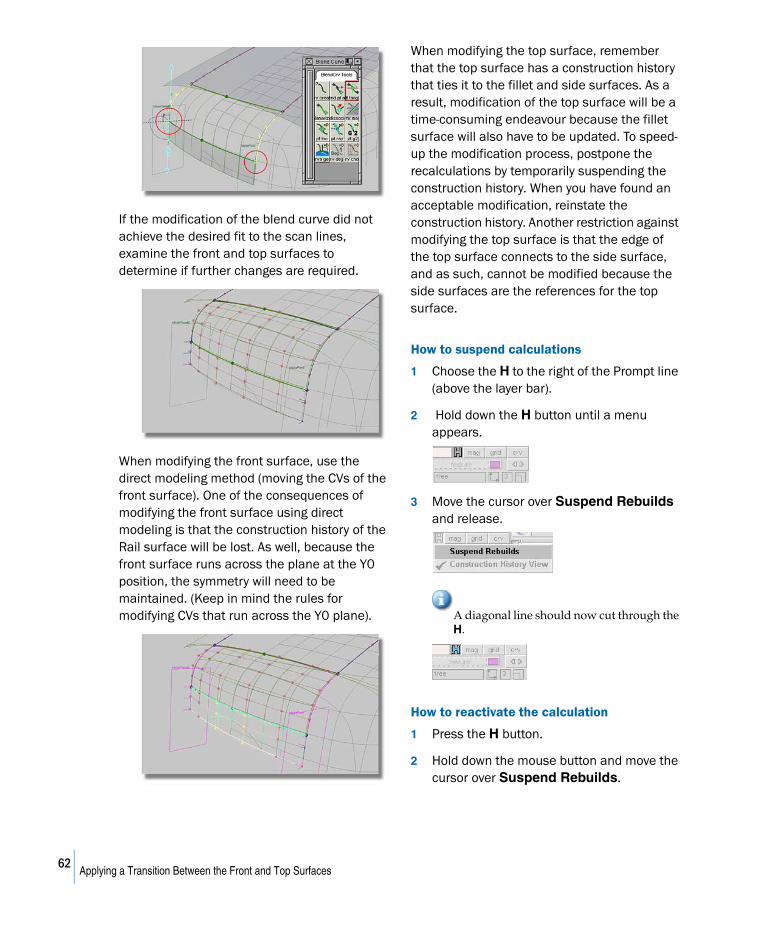
If the modification of the blend curve did not achieve the desired fit to the scan lines, examine the front and top surfaces to determine if further changes are required.
When modifying the front surface, use the direct modeling method (moving the CVs of the front surface). One of the consequences of modifying the front surface using direct modeling is that the construction history of the Rail surface will be lost. As well, because the front surface runs across the plane at the Y0 position, the symmetry will need to be maintained. (Keep in mind the rules for modifying CVs that run across the Y0 plane).
When modifying the top surface, remember that the top surface has a construction history that ties it to the fillet and side surfaces. As a result, modification of the top surface will be a time-consuming endeavour because the fillet surface will also have to be updated. To speed-up the modification process, postpone the recalculations by temporarily suspending the construction history. When you have found an acceptable modification, reinstate the construction history. Another restriction against modifying the top surface is that the edge of the top surface connects to the side surface, and as such, cannot be modified because the side surfaces are the references for the top surface.
How to suspend calculations
1 Choose the H to the right of the Prompt line (above the layer bar).
2 Hold down the H button until a menu appears.
3 Move the cursor over Suspend Rebuilds and release.
A diagonal line should now cut through the H.
How to reactivate the calculation
1 Press the H button.
2 Hold down the mouse button and move the cursor over Suspend Rebuilds.
62Applying a Transition Between the Front and Top Surfaces
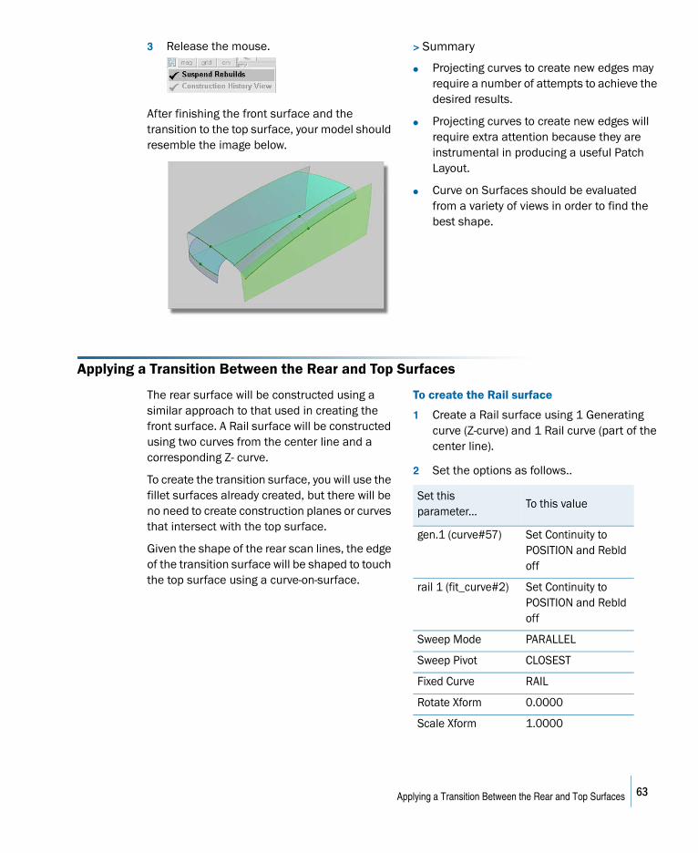
3 Release the mouse.
After finishing the front surface and the transition to the top surface, your model should resemble the image below.
> Summary
● Projecting curves to create new edges may require a number of attempts to achieve the desired results.
● Projecting curves to create new edges will require extra attention because they are instrumental in producing a useful Patch Layout.
● Curve on Surfaces should be evaluated from a variety of views in order to find the best shape.
Applying a Transition Between the Rear and Top Surfaces
The rear surface will be constructed using a similar approach to that used in creating the front surface. A Rail surface will be constructed using two curves from the center line and a corresponding Z- curve.
To create the transition surface, you will use the fillet surfaces already created, but there will be no need to create construction planes or curves that intersect with the top surface.
Given the shape of the rear scan lines, the edge of the transition surface will be shaped to touch the top surface using a curve-on-surface.
To create the Rail surface
1 Create a Rail surface using 1 Generating curve (Z-curve) and 1 Rail curve (part of the center line).
2 Set the options as follows..
Set this parameter...
To this value
gen.1 (curve#57) Set Continuity to POSITION and Rebld off
rail 1 (fit_curve#2) Set Continuity to POSITION and Rebld off
Sweep Mode PARALLEL
Sweep Pivot CLOSEST
Fixed Curve RAIL
Rotate Xform 0.0000
Scale Xform 1.0000
63Applying a Transition Between the Rear and Top Surfaces
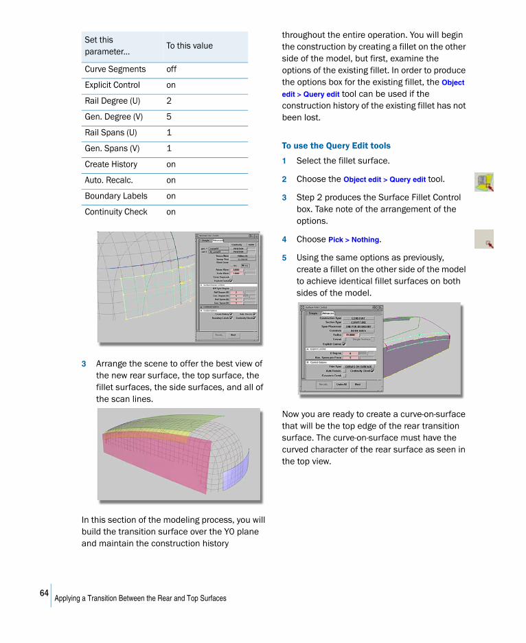
3 Arrange the scene to offer the best view of the new rear surface, the top surface, the fillet surfaces, the side surfaces, and all of the scan lines.
In this section of the modeling process, you will build the transition surface over the Y0 plane and maintain the construction history
throughout the entire operation. You will begin the construction by creating a fillet on the other side of the model, but first, examine the options of the existing fillet. In order to produce the options box for the existing fillet, the Object
edit > Query edit tool can be used if the construction history of the existing fillet has not been lost.
To use the Query Edit tools
1 Select the fillet surface.
2 Choose the Object edit > Query edit tool.
3 Step 2 produces the Surface Fillet Control box. Take note of the arrangement of the options.
4 Choose Pick > Nothing.
5 Using the same options as previously, create a fillet on the other side of the model to achieve identical fillet surfaces on both sides of the model.
Now you are ready to create a curve-on-surface that will be the top edge of the rear transition surface. The curve-on-surface must have the curved character of the rear surface as seen in the top view.
Curve Segments off
Explicit Control on
Rail Degree (U) 2
Gen. Degree (V) 5
Rail Spans (U) 1
Gen. Spans (V) 1
Create History on
Auto. Recalc. on
Boundary Labels on
Continuity Check on
Set this parameter...
To this value
64Applying a Transition Between the Rear and Top Surfaces
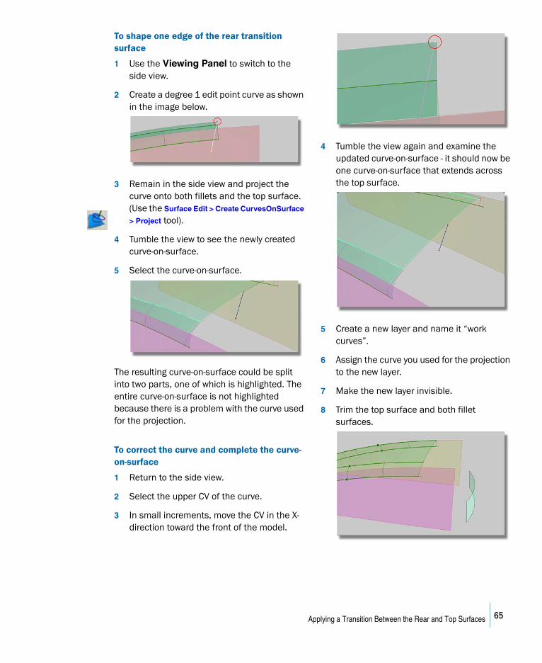
To shape one edge of the rear transition surface
1 Use the Viewing Panel to switch to the side view.
2 Create a degree 1 edit point curve as shown in the image below.
3 Remain in the side view and project the curve onto both fillets and the top surface. (Use the Surface Edit > Create CurvesOnSurface
> Project tool).
4 Tumble the view to see the newly created curve-on-surface.
5 Select the curve-on-surface.
The resulting curve-on-surface could be split into two parts, one of which is highlighted. The entire curve-on-surface is not highlighted because there is a problem with the curve used for the projection.
To correct the curve and complete the curve-on-surface
1 Return to the side view.
2 Select the upper CV of the curve.
3 In small increments, move the CV in the X-direction toward the front of the model.
4 Tumble the view again and examine the updated curve-on-surface - it should now be one curve-on-surface that extends across the top surface.
5 Create a new layer and name it “work curves”.
6 Assign the curve you used for the projection to the new layer.
7 Make the new layer invisible.
8 Trim the top surface and both fillet surfaces.
65Applying a Transition Between the Rear and Top Surfaces
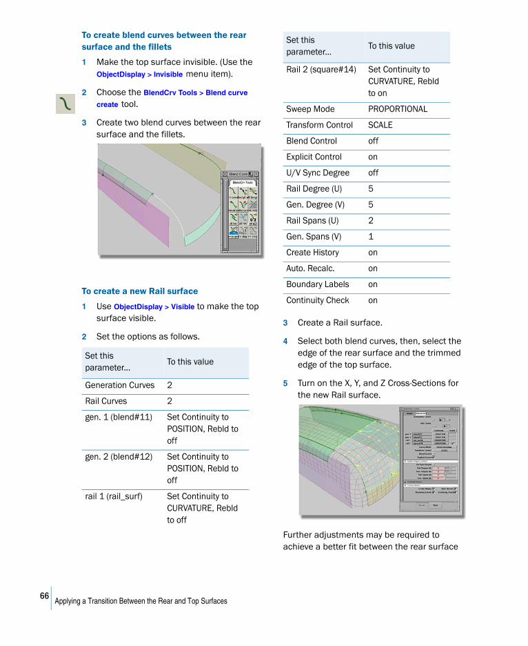
To create blend curves between the rear surface and the fillets
1 Make the top surface invisible. (Use the ObjectDisplay > Invisible menu item).
2 Choose the BlendCrv Tools > Blend curve
create tool.
3 Create two blend curves between the rear surface and the fillets.
To create a new Rail surface
1 Use ObjectDisplay > Visible to make the top surface visible.
2 Set the options as follows.
3 Create a Rail surface.
4 Select both blend curves, then, select the edge of the rear surface and the trimmed edge of the top surface.
5 Turn on the X, Y, and Z Cross-Sections for the new Rail surface.
Further adjustments may be required to achieve a better fit between the rear surface
Set this parameter...
To this value
Generation Curves 2
Rail Curves 2
gen. 1 (blend#11) Set Continuity to POSITION, Rebld to off
gen. 2 (blend#12) Set Continuity to POSITION, Rebld to off
rail 1 (rail_surf) Set Continuity to CURVATURE, Rebld to off
Rail 2 (square#14) Set Continuity to CURVATURE, Rebld to on
Sweep Mode PROPORTIONAL
Transform Control SCALE
Blend Control off
Explicit Control on
U/V Sync Degree off
Rail Degree (U) 5
Gen. Degree (V) 5
Rail Spans (U) 2
Gen. Spans (V) 1
Create History on
Auto. Recalc. on
Boundary Labels on
Continuity Check on
Set this parameter...
To this value
66Applying a Transition Between the Rear and Top Surfaces
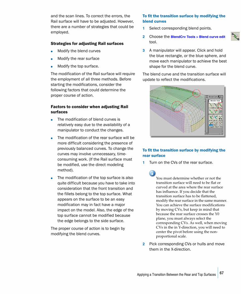
and the scan lines. To correct the errors, the Rail surface will have to be adjusted. However, there are a number of strategies that could be employed.
Strategies for adjusting Rail surfaces
● Modify the blend curves
● Modify the rear surface
● Modify the top surface.
The modification of the Rail surface will require the employment of all three methods. Before starting the modifications, consider the following factors that could determine the proper course of action.
Factors to consider when adjusting Rail surfaces
● The modification of blend curves is relatively easy due to the availability of a manipulator to conduct the changes.
● The modification of the rear surface will be more difficult considering the presence of previously balanced curves. To change the curves may involve unnecessary, time-consuming work. (If the Rail surface must be modified, use the direct modeling method).
● The modification of the top surface is also quite difficult because you have to take into consideration that the front transition and the fillets belong to the top surface. What appears on the surface to be an easy modification may in fact have a major impact on the model. Also, the edge of the top surface cannot be modified because the edge belongs to the side surface.
The proper course of action is to begin by modifying the blend curves.
To fit the transition surface by modifying the blend curves
1 Select corresponding blend points.
2 Choose the BlendCrv Tools > Blend curve edit tool.
3 A manipulator will appear. Click and hold the blue rectangle, or the blue sphere, and move each manipulator to achieve the best shape for the blend curve.
The blend curve and the transition surface will update to reflect the modifications.
To fit the transition surface by modifying the rear surface
1 Turn on the CVs of the rear surface.
You must determine whether or not the transition surface will need to be flat or curved at the area where the rear surface has influence. If you decide that the transition surface has to be flattened, modify the rear surface in the same manner. You can achieve the surface modifications by moving CVs, but keep in mind that because the rear surface crosses the Y0 plane, you must always select the corresponding CVs. As well, when moving CVs in the in Y-direction, you will need to center the pivot before using the non-proportional scale.
2 Pick corresponding CVs or hulls and move them in the X-direction.
67Applying a Transition Between the Rear and Top Surfaces
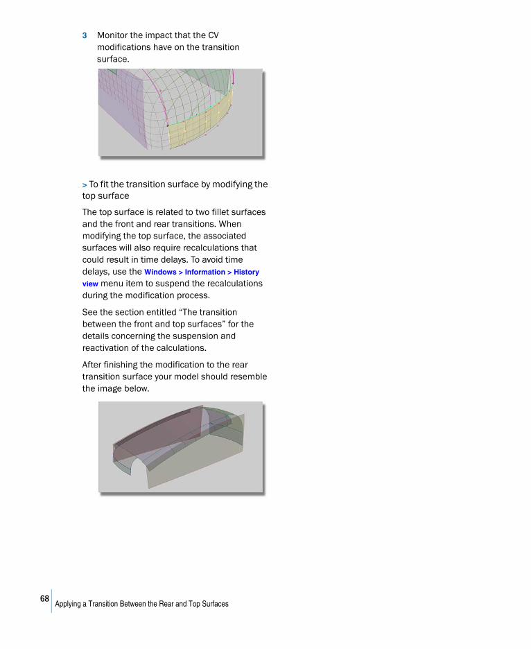
3 Monitor the impact that the CV modifications have on the transition surface.
> To fit the transition surface by modifying the top surface
The top surface is related to two fillet surfaces and the front and rear transitions. When modifying the top surface, the associated surfaces will also require recalculations that could result in time delays. To avoid time delays, use the Windows > Information > History
view menu item to suspend the recalculations during the modification process.
See the section entitled “The transition between the front and top surfaces” for the details concerning the suspension and reactivation of the calculations.
After finishing the modification to the rear transition surface your model should resemble the image below.
68Applying a Transition Between the Rear and Top Surfaces
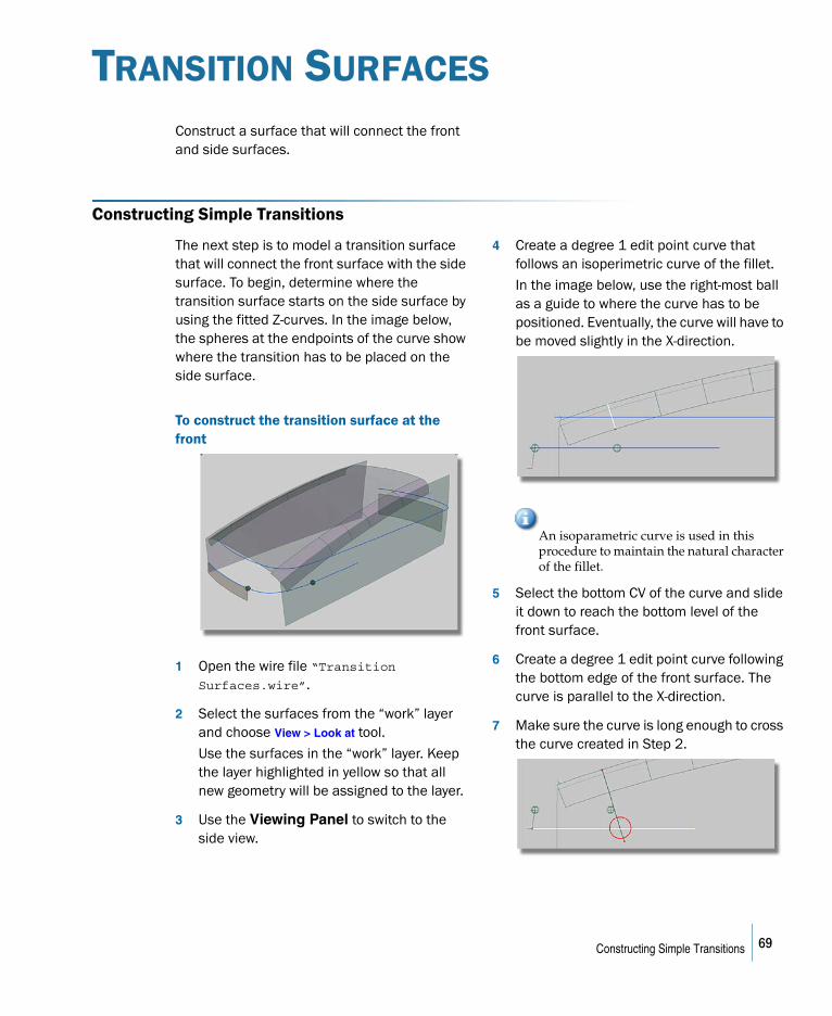
TRANSITION SURFACES
Construct a surface that will connect the front and side surfaces.
Constructing Simple Transitions
The next step is to model a transition surface that will connect the front surface with the side surface. To begin, determine where the transition surface starts on the side surface by using the fitted Z-curves. In the image below, the spheres at the endpoints of the curve show where the transition has to be placed on the side surface.
To construct the transition surface at the front
1 Open the wire file “Transition Surfaces.wire”.
2 Select the surfaces from the “work” layer and choose View > Look at tool.
Use the surfaces in the “work” layer. Keep the layer highlighted in yellow so that all new geometry will be assigned to the layer.
3 Use the Viewing Panel to switch to the side view.
4 Create a degree 1 edit point curve that follows an isoperimetric curve of the fillet.
In the image below, use the right-most ball as a guide to where the curve has to be positioned. Eventually, the curve will have to be moved slightly in the X-direction.
An isoparametric curve is used in this procedure to maintain the natural character of the fillet.
5 Select the bottom CV of the curve and slide it down to reach the bottom level of the front surface.
6 Create a degree 1 edit point curve following the bottom edge of the front surface. The curve is parallel to the X-direction.
7 Make sure the curve is long enough to cross the curve created in Step 2.
69Constructing Simple Transitions
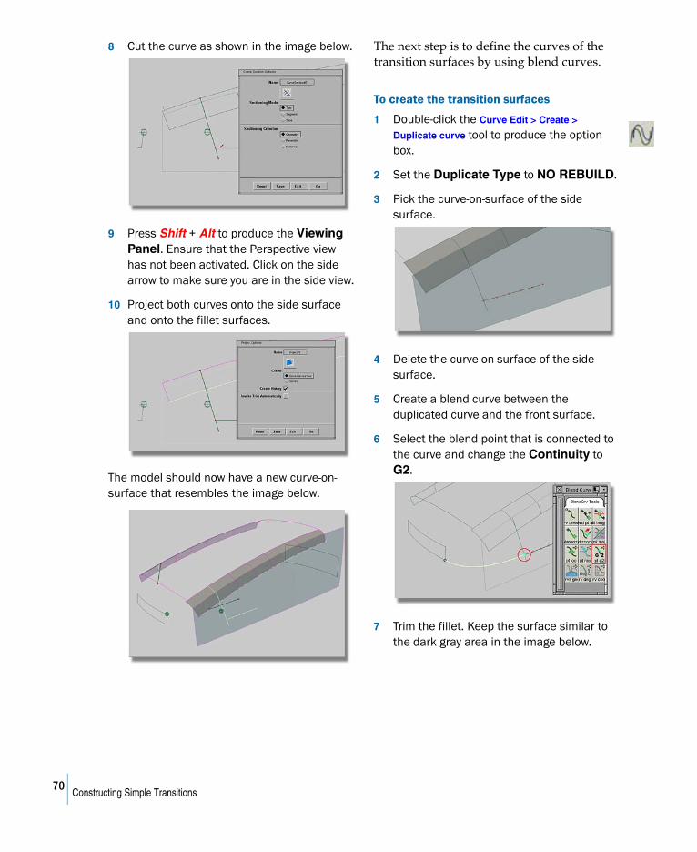
8 Cut the curve as shown in the image below.
9 Press Shift + Alt to produce the Viewing Panel. Ensure that the Perspective view has not been activated. Click on the side arrow to make sure you are in the side view.
10 Project both curves onto the side surface and onto the fillet surfaces.
The model should now have a new curve-on-surface that resembles the image below.
The next step is to define the curves of the transition surfaces by using blend curves.
To create the transition surfaces
1 Double-click the Curve Edit > Create >
Duplicate curve tool to produce the option box.
2 Set the Duplicate Type to NO REBUILD.
3 Pick the curve-on-surface of the side surface.
4 Delete the curve-on-surface of the side surface.
5 Create a blend curve between the duplicated curve and the front surface.
6 Select the blend point that is connected to the curve and change the Continuity to G2.
7 Trim the fillet. Keep the surface similar to the dark gray area in the image below.
70Constructing Simple Transitions
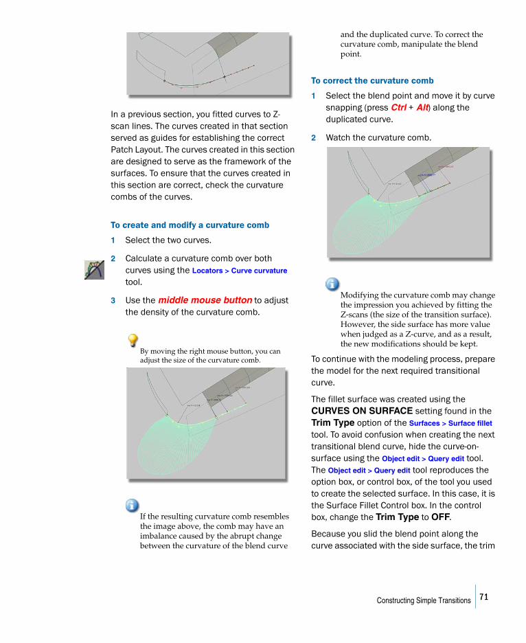
In a previous section, you fitted curves to Z-scan lines. The curves created in that section served as guides for establishing the correct Patch Layout. The curves created in this section are designed to serve as the framework of the surfaces. To ensure that the curves created in this section are correct, check the curvature combs of the curves.
To create and modify a curvature comb
1 Select the two curves.
2 Calculate a curvature comb over both curves using the Locators > Curve curvature tool.
3 Use the middle mouse button to adjust the density of the curvature comb.
By moving the right mouse button, you can adjust the size of the curvature comb.
If the resulting curvature comb resembles the image above, the comb may have an imbalance caused by the abrupt change between the curvature of the blend curve
and the duplicated curve. To correct the curvature comb, manipulate the blend point.
To correct the curvature comb
1 Select the blend point and move it by curve snapping (press Ctrl + Alt) along the duplicated curve.
2 Watch the curvature comb.
Modifying the curvature comb may change the impression you achieved by fitting the Z-scans (the size of the transition surface). However, the side surface has more value when judged as a Z-curve, and as a result, the new modifications should be kept.
To continue with the modeling process, prepare the model for the next required transitional curve.
The fillet surface was created using the CURVES ON SURFACE setting found in the Trim Type option of the Surfaces > Surface fillet tool. To avoid confusion when creating the next transitional blend curve, hide the curve-on-surface using the Object edit > Query edit tool. The Object edit > Query edit tool reproduces the option box, or control box, of the tool you used to create the selected surface. In this case, it is the Surface Fillet Control box. In the control box, change the Trim Type to OFF.
Because you slid the blend point along the curve associated with the side surface, the trim
71Constructing Simple Transitions
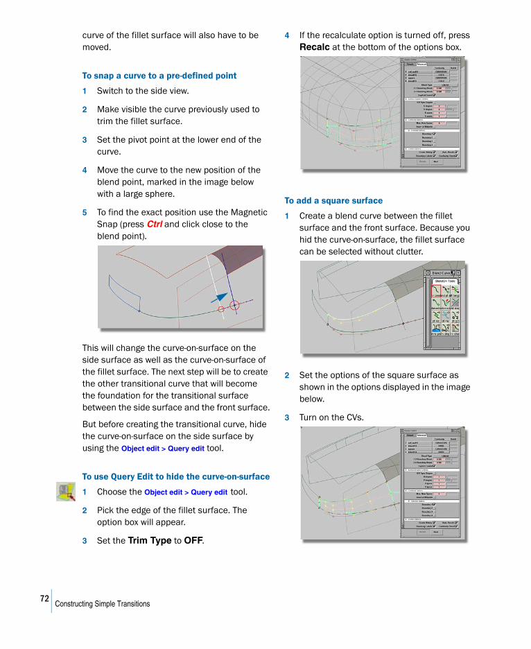
curve of the fillet surface will also have to be moved.
To snap a curve to a pre-defined point
1 Switch to the side view.
2 Make visible the curve previously used to trim the fillet surface.
3 Set the pivot point at the lower end of the curve.
4 Move the curve to the new position of the blend point, marked in the image below with a large sphere.
5 To find the exact position use the Magnetic Snap (press Ctrl and click close to the blend point).
This will change the curve-on-surface on the side surface as well as the curve-on-surface of the fillet surface. The next step will be to create the other transitional curve that will become the foundation for the transitional surface between the side surface and the front surface.
But before creating the transitional curve, hide the curve-on-surface on the side surface by using the Object edit > Query edit tool.
To use Query Edit to hide the curve-on-surface
1 Choose the Object edit > Query edit tool.
2 Pick the edge of the fillet surface. The option box will appear.
3 Set the Trim Type to OFF.
4 If the recalculate option is turned off, press Recalc at the bottom of the options box.
To add a square surface
1 Create a blend curve between the fillet surface and the front surface. Because you hid the curve-on-surface, the fillet surface can be selected without clutter.
2 Set the options of the square surface as shown in the options displayed in the image below.
3 Turn on the CVs.
72Constructing Simple Transitions
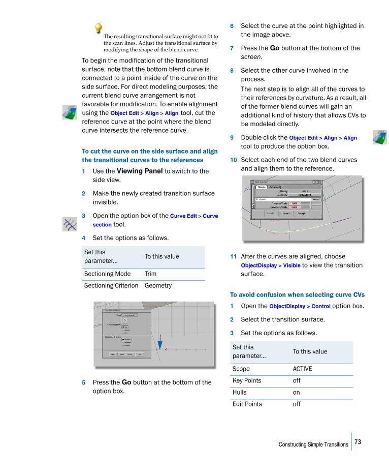
The resulting transitional surface might not fit to the scan lines. Adjust the transitional surface by modifying the shape of the blend curve.
To begin the modification of the transitional surface, note that the bottom blend curve is connected to a point inside of the curve on the side surface. For direct modeling purposes, the current blend curve arrangement is not favorable for modification. To enable alignment using the Object Edit > Align > Align tool, cut the reference curve at the point where the blend curve intersects the reference curve.
To cut the curve on the side surface and align the transitional curves to the references
1 Use the Viewing Panel to switch to the side view.
2 Make the newly created transition surface invisible.
3 Open the option box of the Curve Edit > Curve
section tool.
4 Set the options as follows.
5 Press the Go button at the bottom of the option box.
6 Select the curve at the point highlighted in the image above.
7 Press the Go button at the bottom of the screen.
8 Select the other curve involved in the process.
The next step is to align all of the curves to their references by curvature. As a result, all of the former blend curves will gain an additional kind of history that allows CVs to be modeled directly.
9 Double-click the Object Edit > Align > Align tool to produce the option box.
10 Select each end of the two blend curves and align them to the reference.
11 After the curves are aligned, choose ObjectDisplay > Visible to view the transition surface.
To avoid confusion when selecting curve CVs
1 Open the ObjectDisplay > Control option box.
2 Select the transition surface.
3 Set the options as follows.
Set this parameter...
To this value
Sectioning Mode Trim
Sectioning Criterion Geometry
Set this parameter...
To this value
Scope ACTIVE
Key Points off
Hulls on
Edit Points off
73Constructing Simple Transitions
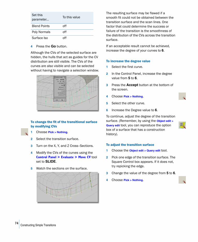
4 Press the Go button.
Although the CVs of the selected surface are hidden, the hulls that act as guides for the CV distribution are still visible. The CVs of the curves are also visible and can be selected without having to navigate a selection window.
To change the fit of the transitional surface by modifying CVs
1 Choose Pick > Nothing.
2 Select the transition surface.
3 Turn on the X, Y, and Z Cross–Sections.
4 Modify the CVs of the curves using the Control Panel > Evaluate > Move CV tool set to SLIDE.
5 Watch the sections on the surface.
The resulting surface may be flawed if a smooth fit could not be obtained between the transition surface and the scan lines. One factor that could determine the success or failure of the transition is the smoothness of the distribution of the CVs across the transition surface.
If an acceptable result cannot be achieved, increase the degree of your curves to 6.
To increase the degree value
1 Select the first curve.
2 In the Control Panel, increase the degree value from 5 to 6.
3 Press the Accept button at the bottom of the screen.
4 Choose Pick > Nothing.
5 Select the other curve.
6 Increase the Degree value to 6.
To continue, adjust the degree of the transition surface. (Remember, by using the Object edit >
Query edit tool, you can reproduce the option box of a surface that has a construction history).
To adjust the transition surface
1 Choose the Object edit > Query edit tool.
2 Pick one edge of the transition surface. The Square Control box appears. If it does not, try repicking the edge.
3 Change the value of the degree from 5 to 6.
4 Choose Pick > Nothing.
Blend Points off
Poly Normals off
Surface Iso off
Set this parameter...
To this value
74Constructing Simple Transitions
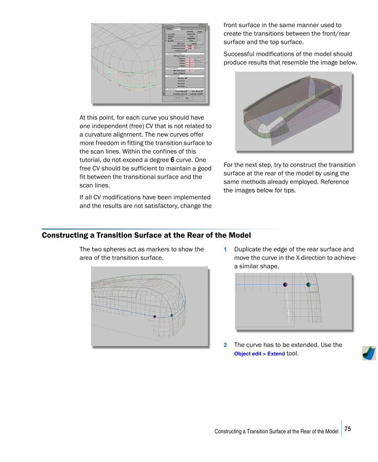
At this point, for each curve you should have one independent (free) CV that is not related to a curvature alignment. The new curves offer more freedom in fitting the transition surface to the scan lines. Within the confines of this tutorial, do not exceed a degree 6 curve. One free CV should be sufficient to maintain a good fit between the transitional surface and the scan lines.
If all CV modifications have been implemented and the results are not satisfactory, change the
front surface in the same manner used to create the transitions between the front/rear surface and the top surface.
Successful modifications of the model should produce results that resemble the image below.
For the next step, try to construct the transition surface at the rear of the model by using the same methods already employed. Reference the images below for tips.
Constructing a Transition Surface at the Rear of the Model
The two spheres act as markers to show the area of the transition surface.
1 Duplicate the edge of the rear surface and move the curve in the X-direction to achieve a similar shape.
2 The curve has to be extended. Use the Object edit > Extend tool.
75Constructing a Transition Surface at the Rear of the Model
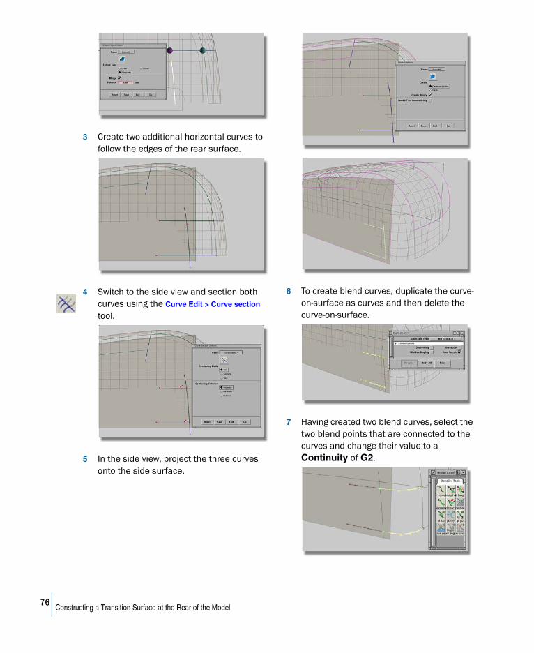
3 Create two additional horizontal curves to follow the edges of the rear surface.
4 Switch to the side view and section both curves using the Curve Edit > Curve section tool.
5 In the side view, project the three curves onto the side surface.
6 To create blend curves, duplicate the curve-on-surface as curves and then delete the curve-on-surface.
7 Having created two blend curves, select the two blend points that are connected to the curves and change their value to a Continuity of G2.
76Constructing a Transition Surface at the Rear of the Model
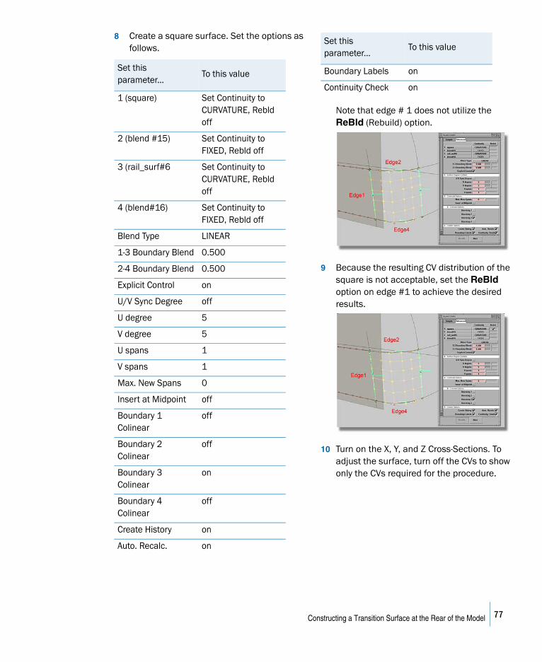
8 Create a square surface. Set the options as follows.
Note that edge # 1 does not utilize the ReBld (Rebuild) option.
9 Because the resulting CV distribution of the square is not acceptable, set the ReBld option on edge #1 to achieve the desired results.
10 Turn on the X, Y, and Z Cross-Sections. To adjust the surface, turn off the CVs to show only the CVs required for the procedure.
Set this parameter...
To this value
1 (square) Set Continuity to CURVATURE, Rebld off
2 (blend #15) Set Continuity to FIXED, Rebld off
3 (rail_surf#6 Set Continuity to CURVATURE, Rebld off
4 (blend#16) Set Continuity to FIXED, Rebld off
Blend Type LINEAR
1-3 Boundary Blend 0.500
2-4 Boundary Blend 0.500
Explicit Control on
U/V Sync Degree off
U degree 5
V degree 5
U spans 1
V spans 1
Max. New Spans 0
Insert at Midpoint off
Boundary 1 Colinear
off
Boundary 2 Colinear
off
Boundary 3 Colinear
on
Boundary 4 Colinear
off
Create History on
Auto. Recalc. on
Boundary Labels on
Continuity Check on
Set this parameter...
To this value
77Constructing a Transition Surface at the Rear of the Model
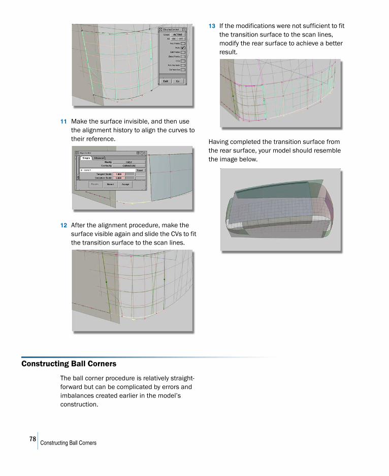
11 Make the surface invisible, and then use the alignment history to align the curves to their reference.
12 After the alignment procedure, make the surface visible again and slide the CVs to fit the transition surface to the scan lines.
13 If the modifications were not sufficient to fit the transition surface to the scan lines, modify the rear surface to achieve a better result.
Having completed the transition surface from the rear surface, your model should resemble the image below.
Constructing Ball Corners
The ball corner procedure is relatively straight-forward but can be complicated by errors and imbalances created earlier in the model’s construction.
78Constructing Ball Corners
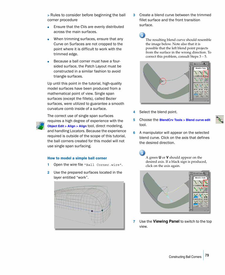
> Rules to consider before beginning the ball corner procedure
● Ensure that the CVs are evenly distributed across the main surfaces.
● When trimming surfaces, ensure that any Curve on Surfaces are not cropped to the point where it is difficult to work with the trimmed edge.
● Because a ball corner must have a four-sided surface, the Patch Layout must be constructed in a similar fashion to avoid triangle surfaces.
Up until this point in the tutorial, high-quality model surfaces have been produced from a mathematical point of view. Single span surfaces (except the fillets), called Bezier surfaces, were utilized to guarantee a smooth curvature comb inside of a surface.
The correct use of single span surfaces requires a high degree of experience with the Object Edit > Align > Align tool, direct modeling, and handling Locators. Because the experience required is outside of the scope of this tutorial, the ball corners created for this model will not use single span surfacing.
How to model a simple ball corner
1 Open the wire file "Ball Corner.wire".
2 Use the prepared surfaces located in the layer entitled “work”.
3 Create a blend curve between the trimmed fillet surface and the front transition surface.
The resulting blend curve should resemble the image below. Note also that it is possible that the left blend point projects from the surface in the wrong direction. To correct this problem, consult Steps 3 – 5.
4 Select the blend point.
5 Choose the BlendCrv Tools > Blend curve edit tool.
6 A manipulator will appear on the selected blend curve. Click on the axis that defines the desired direction.
A green U or V should appear on the desired axis. If a black sign is produced, click on the axis again.
7 Use the Viewing Panel to switch to the top view.
79Constructing Ball Corners
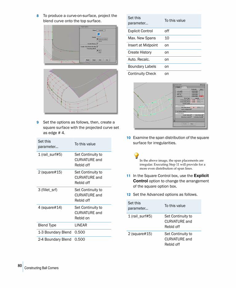
8 To produce a curve-on-surface, project the blend curve onto the top surface.
9 Set the options as follows, then, create a square surface with the projected curve set as edge # 4.
10 Examine the span distribution of the square surface for irregularities.
In the above image, the span placements are irregular. Executing Step 11 will provide for a more even distribution of span lines.
11 In the Square Control box, use the Explicit Control option to change the arrangement of the square option box.
12 Set the Advanced options as follows.
Set this parameter...
To this value
1 (rail_surf#5) Set Continuity to CURVATURE and Rebld off
2 (square#15) Set Continuity to CURVATURE and Rebld off
3 (fillet_srf) Set Continuity to CURVATURE and Rebld off
4 (square#14) Set Continuity to CURVATURE and Rebld on
Blend Type LINEAR
1-3 Boundary Blend 0.500
2-4 Boundary Blend 0.500
Explicit Control off
Max. New Spans 10
Insert at Midpoint on
Create History on
Auto. Recalc. on
Boundary Labels on
Continuity Check on
Set this parameter...
To this value
1 (rail_surf#5) Set Continuity to CURVATURE and Rebld off
2 (square#15) Set Continuity to CURVATURE and Rebld off
Set this parameter...
To this value
80Constructing Ball Corners
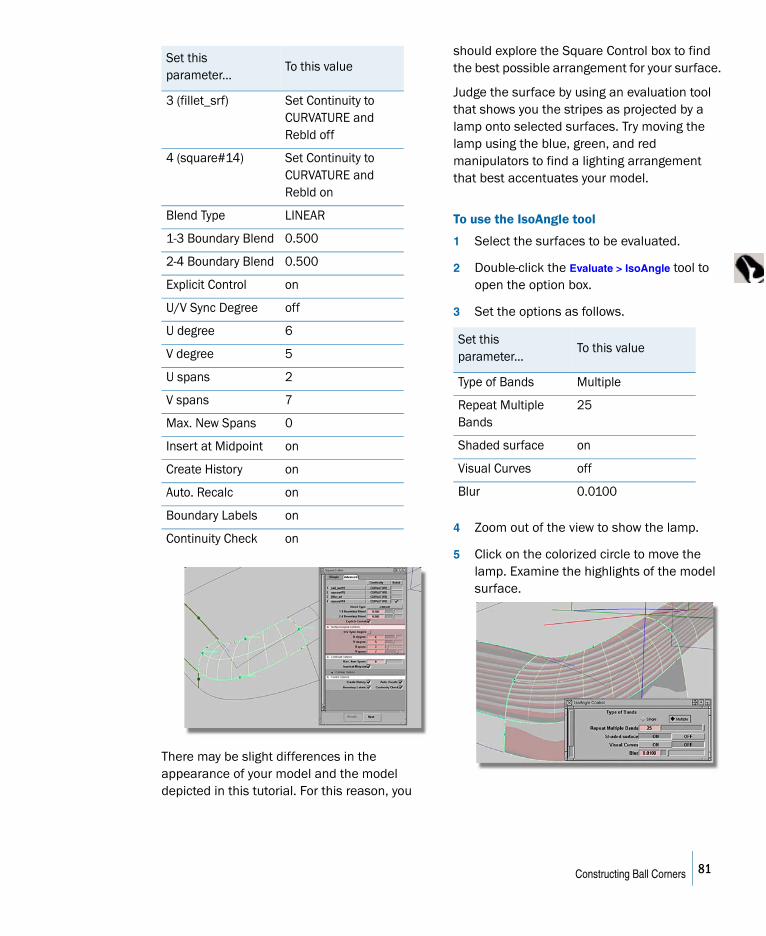
There may be slight differences in the appearance of your model and the model depicted in this tutorial. For this reason, you
should explore the Square Control box to find the best possible arrangement for your surface.
Judge the surface by using an evaluation tool that shows you the stripes as projected by a lamp onto selected surfaces. Try moving the lamp using the blue, green, and red manipulators to find a lighting arrangement that best accentuates your model.
To use the IsoAngle tool
1 Select the surfaces to be evaluated.
2 Double-click the Evaluate > IsoAngle tool to open the option box.
3 Set the options as follows.
4 Zoom out of the view to show the lamp.
5 Click on the colorized circle to move the lamp. Examine the highlights of the model surface.
3 (fillet_srf) Set Continuity to CURVATURE and Rebld off
4 (square#14) Set Continuity to CURVATURE and Rebld on
Blend Type LINEAR
1-3 Boundary Blend 0.500
2-4 Boundary Blend 0.500
Explicit Control on
U/V Sync Degree off
U degree 6
V degree 5
U spans 2
V spans 7
Max. New Spans 0
Insert at Midpoint on
Create History on
Auto. Recalc on
Boundary Labels on
Continuity Check on
Set this parameter...
To this value
Set this parameter...
To this value
Type of Bands Multiple
Repeat Multiple Bands
25
Shaded surface on
Visual Curves off
Blur 0.0100
81Constructing Ball Corners
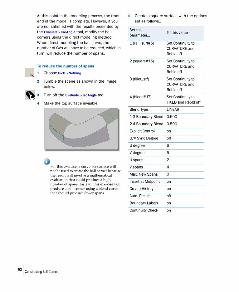
At this point in the modeling process, the front-end of the model is complete. However, if you are not satisfied with the results presented by the Evaluate > IsoAngle tool, modify the ball corners using the direct modeling method. When direct modeling the ball curve, the number of CVs will have to be reduced, which in turn, will reduce the number of spans.
To reduce the number of spans
1 Choose Pick > Nothing.
2 Tumble the scene as shown in the image below.
3 Turn off the Evaluate > IsoAngle tool.
4 Make the top surface invisible.
For this exercise, a curve-on-surface will not be used to create the ball corner because the result will involve a mathematical evaluation that could produce a high number of spans. Instead, this exercise will produce a ball corner using a blend curve that should produce fewer spans.
5 Create a square surface with the options set as follows..
Set this parameter...
To this value
1 (rail_surf#5) Set Continuity to CURVATURE and Rebld off
2 (square#15) Set Continuity to CURVATURE and Rebld off
3 (fillet_srf) Set Continuity to CURVATURE and Rebld off
4 (blend#17) Set Continuity to FIXED and Rebld off
Blend Type LINEAR
1-3 Boundary Blend 0.500
2-4 Boundary Blend 0.500
Explicit Control on
U/V Sync Degree off
U degree 6
V degree 5
U spans 2
V spans 4
Max. New Spans 0
Insert at Midpoint on
Create History on
Auto. Recalc off
Boundary Labels on
Continuity Check on
82Constructing Ball Corners
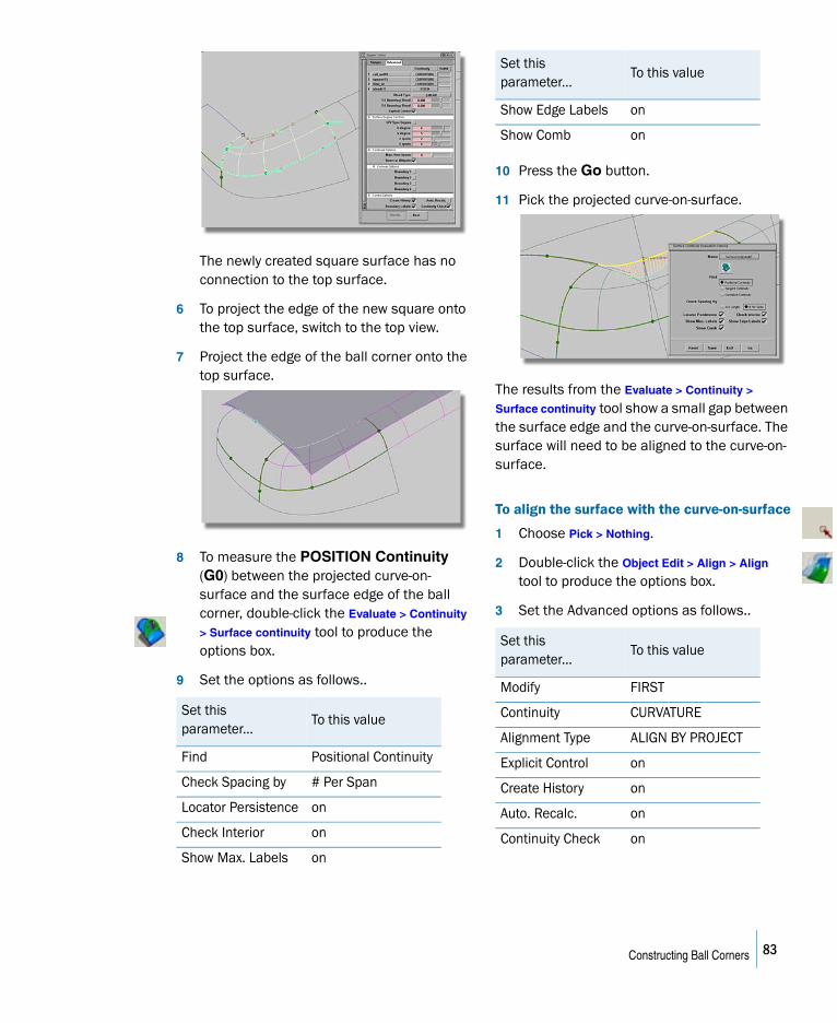
The newly created square surface has no connection to the top surface.
6 To project the edge of the new square onto the top surface, switch to the top view.
7 Project the edge of the ball corner onto the top surface.
8 To measure the POSITION Continuity (G0) between the projected curve-on-surface and the surface edge of the ball corner, double-click the Evaluate > Continuity
> Surface continuity tool to produce the options box.
9 Set the options as follows..
10 Press the Go button.
11 Pick the projected curve-on-surface.
The results from the Evaluate > Continuity >
Surface continuity tool show a small gap between the surface edge and the curve-on-surface. The surface will need to be aligned to the curve-on-surface.
To align the surface with the curve-on-surface
1 Choose Pick > Nothing.
2 Double-click the Object Edit > Align > Align tool to produce the options box.
3 Set the Advanced options as follows..
Set this parameter...
To this value
Find Positional Continuity
Check Spacing by # Per Span
Locator Persistence on
Check Interior on
Show Max. Labels on
Show Edge Labels on
Show Comb on
Set this parameter...
To this value
Modify FIRST
Continuity CURVATURE
Alignment Type ALIGN BY PROJECT
Explicit Control on
Create History on
Auto. Recalc. on
Continuity Check on
Set this parameter...
To this value
83Constructing Ball Corners
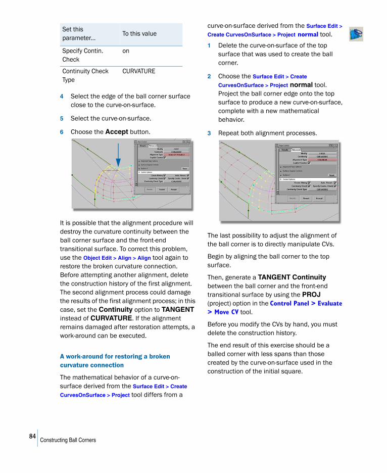
4 Select the edge of the ball corner surface close to the curve-on-surface.
5 Select the curve-on-surface.
6 Choose the Accept button.
It is possible that the alignment procedure will destroy the curvature continuity between the ball corner surface and the front-end transitional surface. To correct this problem, use the Object Edit > Align > Align tool again to restore the broken curvature connection. Before attempting another alignment, delete the construction history of the first alignment. The second alignment process could damage the results of the first alignment process; in this case, set the Continuity option to TANGENT instead of CURVATURE. If the alignment remains damaged after restoration attempts, a work-around can be executed.
A work-around for restoring a broken curvature connection
The mathematical behavior of a curve-on-surface derived from the Surface Edit > Create
CurvesOnSurface > Project tool differs from a
curve-on-surface derived from the Surface Edit >
Create CurvesOnSurface > Project normal tool.
1 Delete the curve-on-surface of the top surface that was used to create the ball corner.
2 Choose the Surface Edit > Create
CurvesOnSurface > Project normal tool. Project the ball corner edge onto the top surface to produce a new curve-on-surface, complete with a new mathematical behavior.
3 Repeat both alignment processes.
The last possibility to adjust the alignment of the ball corner is to directly manipulate CVs.
Begin by aligning the ball corner to the top surface.
Then, generate a TANGENT Continuity between the ball corner and the front-end transitional surface by using the PROJ (project) option in the Control Panel > Evaluate > Move CV tool.
Before you modify the CVs by hand, you must delete the construction history.
The end result of this exercise should be a balled corner with less spans than those created by the curve-on-surface used in the construction of the initial square.
Specify Contin. Check
on
Continuity Check Type
CURVATURE
Set this parameter...
To this value
84Constructing Ball Corners
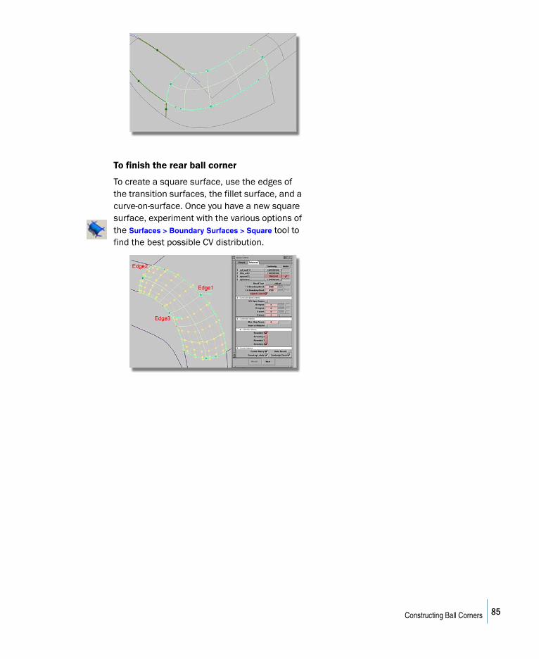
To finish the rear ball corner
To create a square surface, use the edges of the transition surfaces, the fillet surface, and a curve-on-surface. Once you have a new square surface, experiment with the various options of the Surfaces > Boundary Surfaces > Square tool to find the best possible CV distribution.
85Constructing Ball Corners

86Constructing Ball Corners
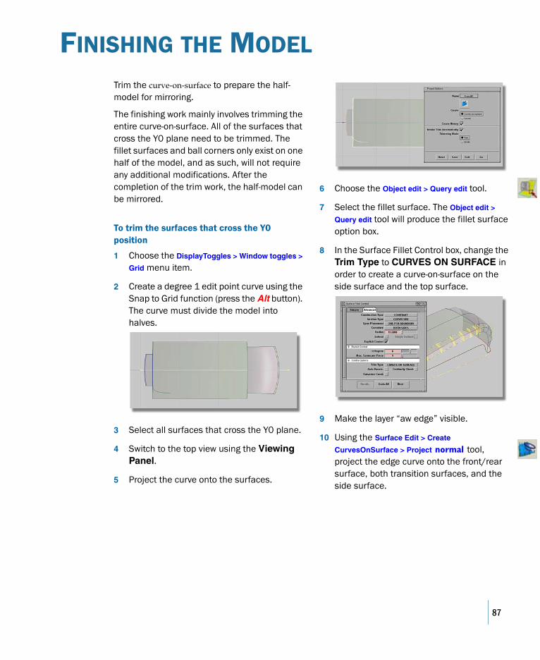
FINISHING THE MODEL
Trim the curve-on-surface to prepare the half-model for mirroring.
The finishing work mainly involves trimming the entire curve-on-surface. All of the surfaces that cross the Y0 plane need to be trimmed. The fillet surfaces and ball corners only exist on one half of the model, and as such, will not require any additional modifications. After the completion of the trim work, the half-model can be mirrored.
To trim the surfaces that cross the Y0 position
1 Choose the DisplayToggles > Window toggles >
Grid menu item.
2 Create a degree 1 edit point curve using the Snap to Grid function (press the Alt button). The curve must divide the model into halves.
3 Select all surfaces that cross the Y0 plane.
4 Switch to the top view using the Viewing Panel.
5 Project the curve onto the surfaces.
6 Choose the Object edit > Query edit tool.
7 Select the fillet surface. The Object edit >
Query edit tool will produce the fillet surface option box.
8 In the Surface Fillet Control box, change the Trim Type to CURVES ON SURFACE in order to create a curve-on-surface on the side surface and the top surface.
9 Make the layer “aw edge” visible.
10 Using the Surface Edit > Create
CurvesOnSurface > Project normal tool, project the edge curve onto the front/rear surface, both transition surfaces, and the side surface.
87
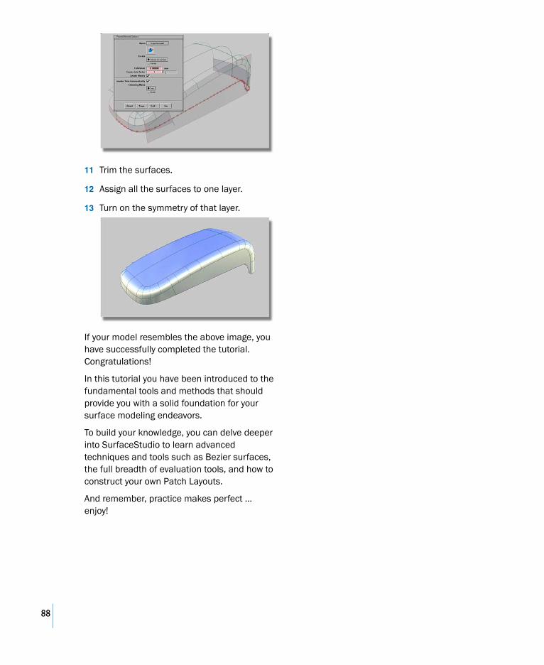
11 Trim the surfaces.
12 Assign all the surfaces to one layer.
13 Turn on the symmetry of that layer.
If your model resembles the above image, you have successfully completed the tutorial. Congratulations!
In this tutorial you have been introduced to the fundamental tools and methods that should provide you with a solid foundation for your surface modeling endeavors.
To build your knowledge, you can delve deeper into SurfaceStudio to learn advanced techniques and tools such as Bezier surfaces, the full breadth of evaluation tools, and how to construct your own Patch Layouts.
And remember, practice makes perfect … enjoy!
88
ADVANCED SURFACE MODELING
Learning objectives
In this overview, you will gain an understanding of the critical tools required for class A surfacing, and will gain control over the quality of surfaces built by using the surface evaluation tools.
An overview of the core competencies required for advanced surface modeling.
In the Foundations of Surface Modeling tutorial you were exposed to the degree of craftsmanship required of a surface modeler. And you were introduced to SurfaceStudio, your new tool that allows you to perform surface modeling in the same manner as traditional methods. You may have traded in the workshop for a virtual space, but the core competencies of surface modeling are still the same.
Required competencies for mastering the craft of surface modeling
● the core tools
● the character of the material to be worked (wood, leather, steel)
● the critical evaluation of the finished work
To provide you with the tools and knowledge necessary to become a master craftsman in the arena of surface modeling, the following topics will be addressed in this tutorial:
Master the Critical Tools
● Blend curves
● Align Tool
● Surface Fillets
Master the Geometry Elements
● NURBS vs. Bezier surfaces
89
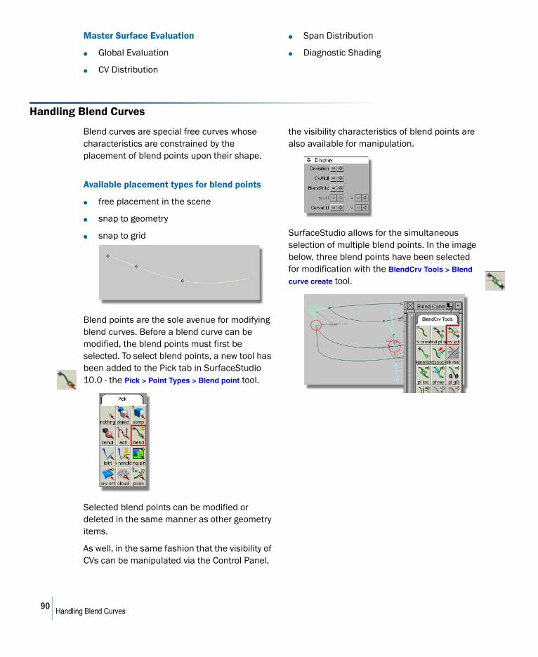
Master Surface Evaluation
● Global Evaluation
● CV Distribution
● Span Distribution
● Diagnostic Shading
Handling Blend Curves
Blend curves are special free curves whose characteristics are constrained by the placement of blend points upon their shape.
Available placement types for blend points
● free placement in the scene
● snap to geometry
● snap to grid
Blend points are the sole avenue for modifying blend curves. Before a blend curve can be modified, the blend points must first be selected. To select blend points, a new tool has been added to the Pick tab in SurfaceStudio 10.0 - the Pick > Point Types > Blend point tool.
Selected blend points can be modified or deleted in the same manner as other geometry items.
As well, in the same fashion that the visibility of CVs can be manipulated via the Control Panel,
the visibility characteristics of blend points are also available for manipulation.
SurfaceStudio allows for the simultaneous selection of multiple blend points. In the image below, three blend points have been selected for modification with the BlendCrv Tools > Blend
curve create tool.
90Handling Blend Curves
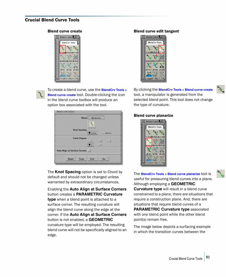
Crucial Blend Curve Tools
Blend curve create
To create a blend curve, use the BlendCrv Tools >
Blend curve create tool. Double-clicking the icon in the blend curve toolbox will produce an option box associated with the tool.
The Knot Spacing option is set to Chord by default and should not be changed unless warranted by extraordinary circumstances.
Enabling the Auto Align at Surface Corners button creates a PARAMETRIC Curvature type when a blend point is attached to a surface corner. The resulting curvature will align the blend curve along the edge at the corner. If the Auto Align at Surface Corners button is not enabled, a GEOMETRIC curvature type will be employed. The resulting blend curve will not be specifically aligned to an edge.
Blend curve edit tangent
By clicking the BlendCrv Tools > Blend curve create tool, a manipulator is generated from the selected blend point. This tool does not change the type of curvature.
Blend curve planarize
The BlendCrv Tools > Blend curve planarize tool is useful for pressuring blend curves into a plane. Although employing a GEOMETRIC Curvature type will result in a blend curve constrained to a plane, there are situations that require a construction plane. And, there are situations that require blend curves of a PARAMETRIC Curvature type associated with one blend point while the other blend point(s) remain free.
The image below depicts a surfacing example in which the transition curves between the
91Crucial Blend Curve Tools
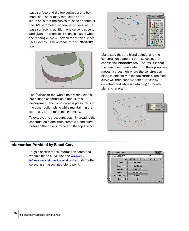
base surface and the top surface are to be modeled. The primary restriction of the situation is that the curves must be oriented at the U/V parameter (isoperimetric lines) of the base surface. In addition, one curve is absent, and given the example, it is unclear as to where the missing curve will attach to the top surface. This example is tailor-made for the Planarize tool.
The Planarize tool works best when using a pre-defined construction plane. In this arrangement, the blend curve is pressured into the construction plane while maintaining the continuity of the reference geometry.
To execute this procedure, begin by creating the construction plane, then create a blend curve between the base surface and the top surface.
Make sure that the blend point(s) and the construction plane are both selected, then choose the Planarize tool. The result is that the blend point associated with the top surface moves to a position where the construction plane intersects with the top surface. The blend curve will then connect both surfaces by curvature and while maintaining a smooth planar character.
Information Provided by Blend Curves
To gain access to the information contained within a blend curve, use the Windows >
Information > Information window menu item after selecting an associated blend point.
Intersection
92Information Provided by Blend Curves
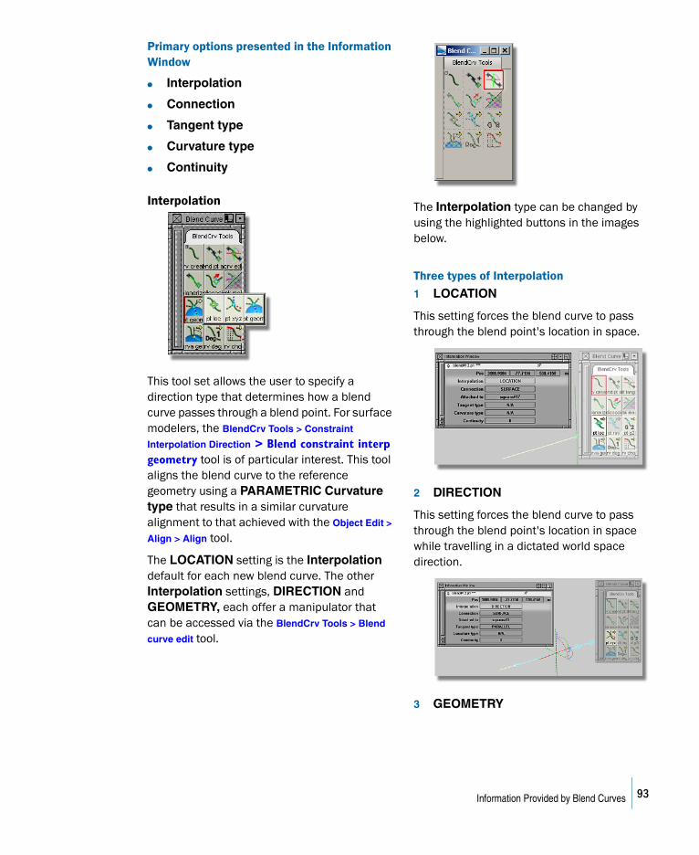
Primary options presented in the Information Window
● Interpolation
● Connection
● Tangent type
● Curvature type
● Continuity
Interpolation
This tool set allows the user to specify a direction type that determines how a blend curve passes through a blend point. For surface modelers, the BlendCrv Tools > Constraint
Interpolation Direction > Blend constraint interp geometry tool is of particular interest. This tool aligns the blend curve to the reference geometry using a PARAMETRIC Curvature type that results in a similar curvature alignment to that achieved with the Object Edit >
Align > Align tool.
The LOCATION setting is the Interpolation default for each new blend curve. The other Interpolation settings, DIRECTION and GEOMETRY, each offer a manipulator that can be accessed via the BlendCrv Tools > Blend
curve edit tool.
The Interpolation type can be changed by using the highlighted buttons in the images below.
Three types of Interpolation
1 LOCATION
This setting forces the blend curve to pass through the blend point's location in space.
2 DIRECTION
This setting forces the blend curve to pass through the blend point's location in space while travelling in a dictated world space direction.
3 GEOMETRY
93Information Provided by Blend Curves
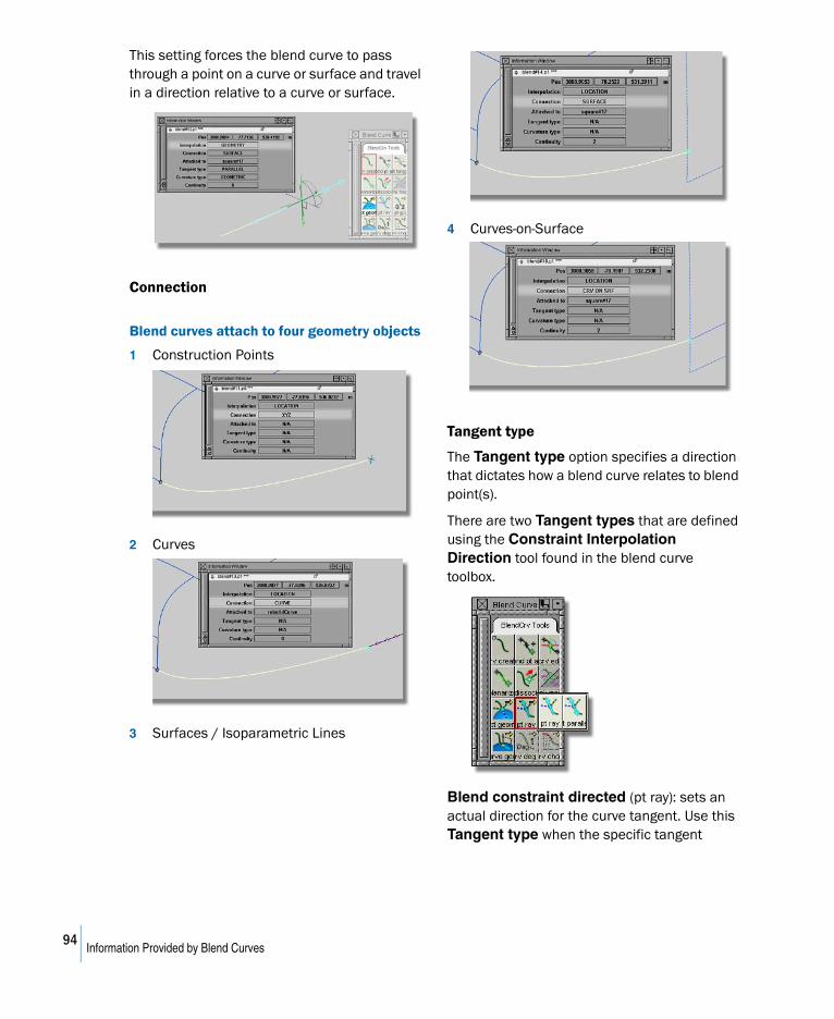
This setting forces the blend curve to pass through a point on a curve or surface and travel in a direction relative to a curve or surface.
Connection
Blend curves attach to four geometry objects
1 Construction Points
2 Curves
3 Surfaces / Isoparametric Lines
4 Curves-on-Surface
Tangent type
The Tangent type option specifies a direction that dictates how a blend curve relates to blend point(s).
There are two Tangent types that are defined using the Constraint Interpolation Direction tool found in the blend curve toolbox.
Blend constraint directed (pt ray): sets an actual direction for the curve tangent. Use this Tangent type when the specific tangent
94Information Provided by Blend Curves
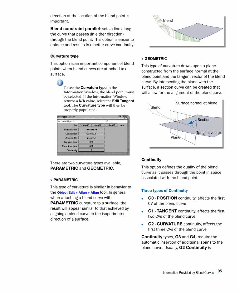
direction at the location of the blend point is important.
Blend constraint parallel: sets a line along the curve that passes (in either direction) through the blend point. This option is easier to enforce and results in a better curve continuity.
Curvature type
This option is an important component of blend points when blend curves are attached to a surface.
To see the Curvature type in the Information Window, the blend point must be selected. If the Information Window returns a N/A value, select the Edit Tangent tool. The Curvature type will then be properly populated.
There are two curvature types available, PARAMETRIC and GEOMETRIC.
> PARAMETRIC
This type of curvature is similar in behavior to the Object Edit > Align > Align tool. In general, when attaching a blend curve with PARAMETRIC curvature to a surface, the result will appear similar to that achieved by aligning a blend curve to the isoperimetric direction of a surface.
> GEOMETRIC
This type of curvature draws upon a plane constructed from the surface normal at the blend point and the tangent vector of the blend curve. By intersecting the plane with the surface, a section curve can be created that will allow for the alignment of the blend curve.
Continuity
This option defines the quality of the blend curve as it passes through the point in space associated with the blend point.
Three types of Continuity
● G0 - POSITION continuity, affects the first CV of the blend curve
● G1 - TANGENT continuity, affects the first two CVs of the blend curve
● G2 - CURVATURE continuity, affects the first three CVs of the blend curve
Continuity types, G3 and G4, require the automatic insertion of additional spans to the blend curve. Usually, G2 Continuity is
Blend
Blend Surface normal at blend
Section
Tangent vector Plane
95Information Provided by Blend Curves
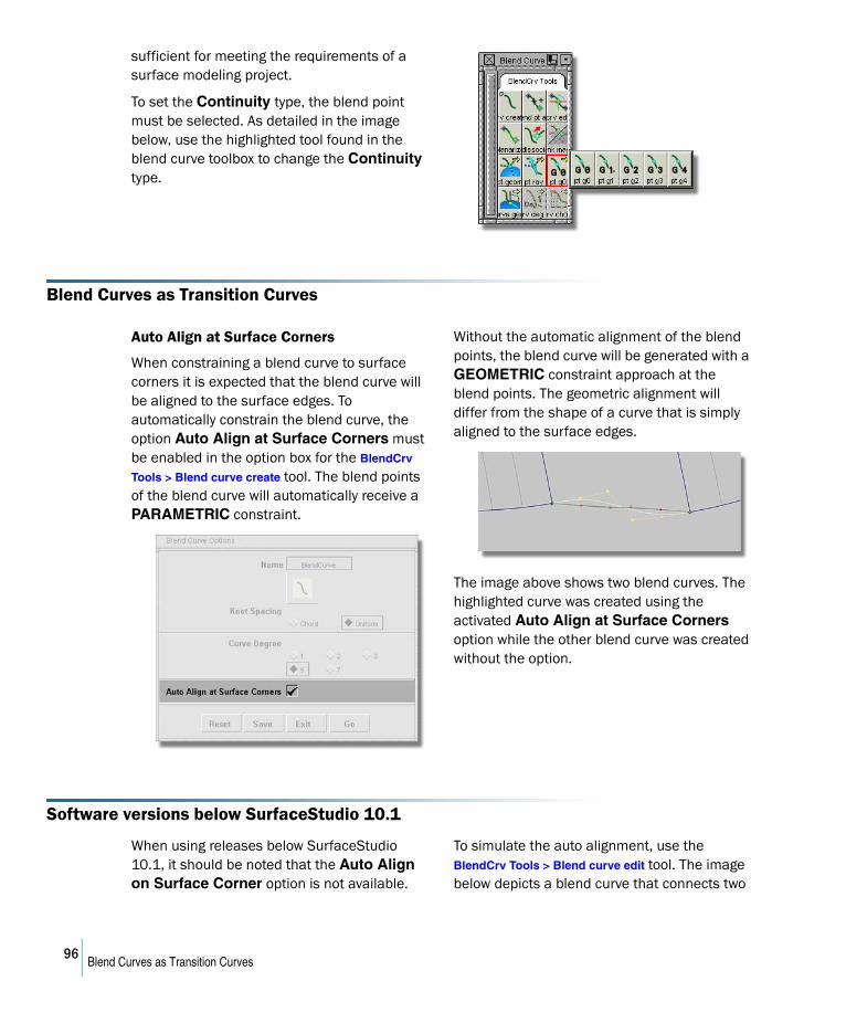
sufficient for meeting the requirements of a surface modeling project.
To set the Continuity type, the blend point must be selected. As detailed in the image below, use the highlighted tool found in the blend curve toolbox to change the Continuity type.
Blend Curves as Transition Curves
Auto Align at Surface Corners
When constraining a blend curve to surface corners it is expected that the blend curve will be aligned to the surface edges. To automatically constrain the blend curve, the option Auto Align at Surface Corners must be enabled in the option box for the BlendCrv
Tools > Blend curve create tool. The blend points of the blend curve will automatically receive a PARAMETRIC constraint.
Without the automatic alignment of the blend points, the blend curve will be generated with a GEOMETRIC constraint approach at the blend points. The geometric alignment will differ from the shape of a curve that is simply aligned to the surface edges.
The image above shows two blend curves. The highlighted curve was created using the activated Auto Align at Surface Corners option while the other blend curve was created without the option.
Software versions below SurfaceStudio 10.1
When using releases below SurfaceStudio 10.1, it should be noted that the Auto Align on Surface Corner option is not available.
To simulate the auto alignment, use the BlendCrv Tools > Blend curve edit tool. The image below depicts a blend curve that connects two
96Blend Curves as Transition Curves
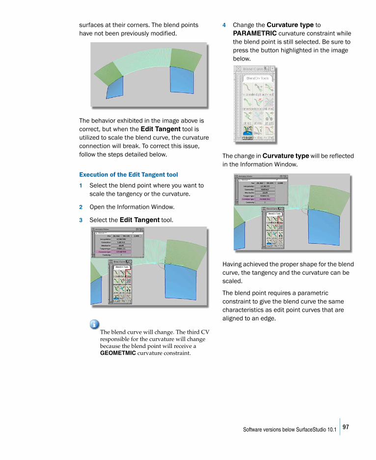
surfaces at their corners. The blend points have not been previously modified.
The behavior exhibited in the image above is correct, but when the Edit Tangent tool is utilized to scale the blend curve, the curvature connection will break. To correct this issue, follow the steps detailed below.
Execution of the Edit Tangent tool
1 Select the blend point where you want to scale the tangency or the curvature.
2 Open the Information Window.
3 Select the Edit Tangent tool.
The blend curve will change. The third CV responsible for the curvature will change because the blend point will receive a GEOMETMIC curvature constraint.
4 Change the Curvature type to PARAMETRIC curvature constraint while the blend point is still selected. Be sure to press the button highlighted in the image below.
The change in Curvature type will be reflected in the Information Window.
Having achieved the proper shape for the blend curve, the tangency and the curvature can be scaled.
The blend point requires a parametric constraint to give the blend curve the same characteristics as edit point curves that are aligned to an edge.
97Software versions below SurfaceStudio 10.1
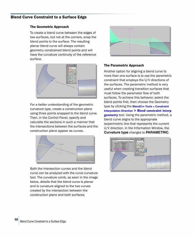
Blend Curve Constraint to a Surface Edge
The Geometric Approach
To create a blend curve between the edges of two surfaces, but not at the corners, snap the blend points to the surface. The resulting planar blend curve will always contain geometry constrained blend points and will have the curvature continuity of the reference surface.
For a better understanding of the geometric curvature type, create a construction plane using three points snapped to the blend curve. Then, in the Control Panel, specify and calculate the sections in such a manner that the intersections between the surfaces and the construction plane appear as curves.
Both the intersection curves and the blend curve can be analyzed with the curve curvature tool. The curvature comb, as seen in the image below, details that the blend curve is planar and is curvature aligned to the two curves created by the intersection between the construction plane and both surfaces.
The Parametric Approach
Another option for aligning a blend curve to more than one surface is to use the parametric constraint that employs the U/V directions of the surfaces. The parametric method is very useful when creating transition surfaces that must follow the parameter flow of both surfaces. To achieve this behavior, select the blend points first, then choose the Geometry type by clicking the BlendCrv Tools > Constraint
Interpolation Direction > Blend constraint interp geometry tool. Using the parametric method, a blend curve aligns to the appropriate isoperimetric line that represents the current U/V direction. In the Information Window, the Curvature type changes to PARAMETRIC.
98Blend Curve Constraint to a Surface Edge
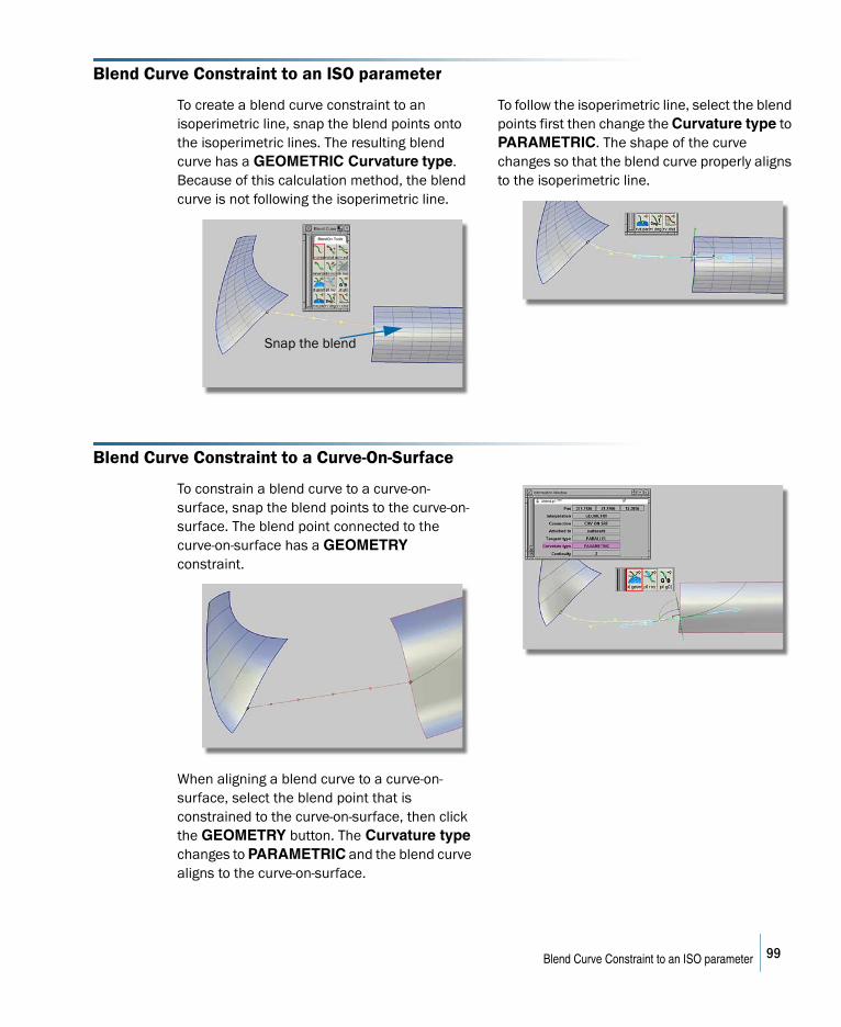
Blend Curve Constraint to an ISO parameter
To create a blend curve constraint to an isoperimetric line, snap the blend points onto the isoperimetric lines. The resulting blend curve has a GEOMETRIC Curvature type. Because of this calculation method, the blend curve is not following the isoperimetric line.
To follow the isoperimetric line, select the blend points first then change the Curvature type to PARAMETRIC. The shape of the curve changes so that the blend curve properly aligns to the isoperimetric line.
Blend Curve Constraint to a Curve-On-Surface
To constrain a blend curve to a curve-on-surface, snap the blend points to the curve-on-surface. The blend point connected to the curve-on-surface has a GEOMETRY constraint.
When aligning a blend curve to a curve-on-surface, select the blend point that is constrained to the curve-on-surface, then click the GEOMETRY button. The Curvature type changes to PARAMETRIC and the blend curve aligns to the curve-on-surface.
Snap the blend
99Blend Curve Constraint to an ISO parameter
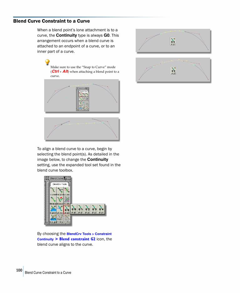
Blend Curve Constraint to a Curve
When a blend point’s lone attachment is to a curve, the Continuity type is always G0. This arrangement occurs when a blend curve is attached to an endpoint of a curve, or to an inner part of a curve.
Make sure to use the “Snap to Curve” mode (Ctrl + Alt) when attaching a blend point to a curve.
To align a blend curve to a curve, begin by selecting the blend point(s). As detailed in the image below, to change the Continuity setting, use the expanded tool set found in the blend curve toolbox.
By choosing the BlendCrv Tools > Constraint
Continuity > Blend constraint G2 icon, the blend curve aligns to the curve.
100Blend Curve Constraint to a Curve
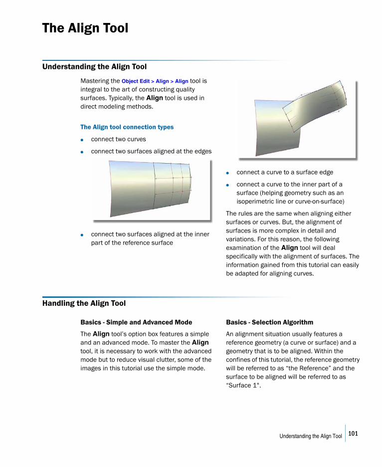
The Align Tool
Understanding the Align Tool
Mastering the Object Edit > Align > Align tool is integral to the art of constructing quality surfaces. Typically, the Align tool is used in direct modeling methods.
The Align tool connection types
● connect two curves
● connect two surfaces aligned at the edges
● connect two surfaces aligned at the inner part of the reference surface
● connect a curve to a surface edge
● connect a curve to the inner part of a surface (helping geometry such as an isoperimetric line or curve-on-surface)
The rules are the same when aligning either surfaces or curves. But, the alignment of surfaces is more complex in detail and variations. For this reason, the following examination of the Align tool will deal specifically with the alignment of surfaces. The information gained from this tutorial can easily be adapted for aligning curves.
Handling the Align Tool
Basics - Simple and Advanced Mode
The Align tool’s option box features a simple and an advanced mode. To master the Align tool, it is necessary to work with the advanced mode but to reduce visual clutter, some of the images in this tutorial use the simple mode.
Basics - Selection Algorithm
An alignment situation usually features a reference geometry (a curve or surface) and a geometry that is to be aligned. Within the confines of this tutorial, the reference geometry will be referred to as “the Reference” and the surface to be aligned will be referred to as “Surface 1".
101Understanding the Align Tool
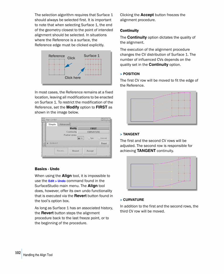
The selection algorithm requires that Surface 1 should always be selected first. It is important to note that when selecting Surface 1, the end of the geometry closest to the point of intended alignment should be selected. In situations where the Reference is a surface, the Reference edge must be clicked explicitly.
In most cases, the Reference remains at a fixed location, leaving all modifications to be enacted on Surface 1. To restrict the modification of the Reference, set the Modify option to FIRST as shown in the image below.
Basics - Undo
When using the Align tool, it is impossible to use the Edit > Undo command found in the SurfaceStudio main menu. The Align tool does, however, offer its own undo functionality that is executed via the Revert button found in the tool’s option box.
As long as Surface 1 has an associated history, the Revert button steps the alignment procedure back to the last freeze point, or to the beginning of the procedure.
Clicking the Accept button freezes the alignment procedure.
Continuity
The Continuity option dictates the quality of the alignment.
The execution of the alignment procedure changes the CV distribution of Surface 1. The number of influenced CVs depends on the quality set in the Continuity option.
> POSITION
The first CV row will be moved to fit the edge of the Reference.
> TANGENT
The first and the second CV rows will be adjusted. The second row is responsible for achieving TANGENT continuity.
> CURVATURE
In addition to the first and the second rows, the third CV row will be moved.
Reference Surface 1Click
Click here
102Handling the Align Tool
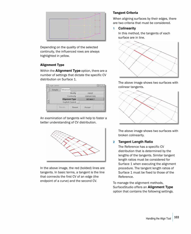
Depending on the quality of the selected continuity, the influenced rows are always highlighted in yellow.
Alignment Type
Within the Alignment Type option, there are a number of settings that dictate the specific CV distribution on Surface 1.
An examination of tangents will help to foster a better understanding of CV distribution.
In the above image, the red (bolded) lines are tangents. In basic terms, a tangent is the line that connects the first CV of an edge (the endpoint of a curve) and the second CV.
Tangent Criteria
When aligning surfaces by their edges, there are two criteria that must be considered.
1 ColinearityIn this method, the tangents of each surface are in line.
The above image shows two surfaces with colinear tangents.
The above image shows two surfaces with broken colinearity.
2 Tangent Length RatioThe Reference has a specific CV distribution that is determined by the lengths of the tangents. Similar tangent length ratios must be considered for Surface 1 when executing the alignment procedure. The tangent length ratios of Surface 1 must be fixed to those of the Reference.
To manage the alignment methods, SurfaceStudio offers an Alignment Type option that contains the following settings.
103Handling the Align Tool
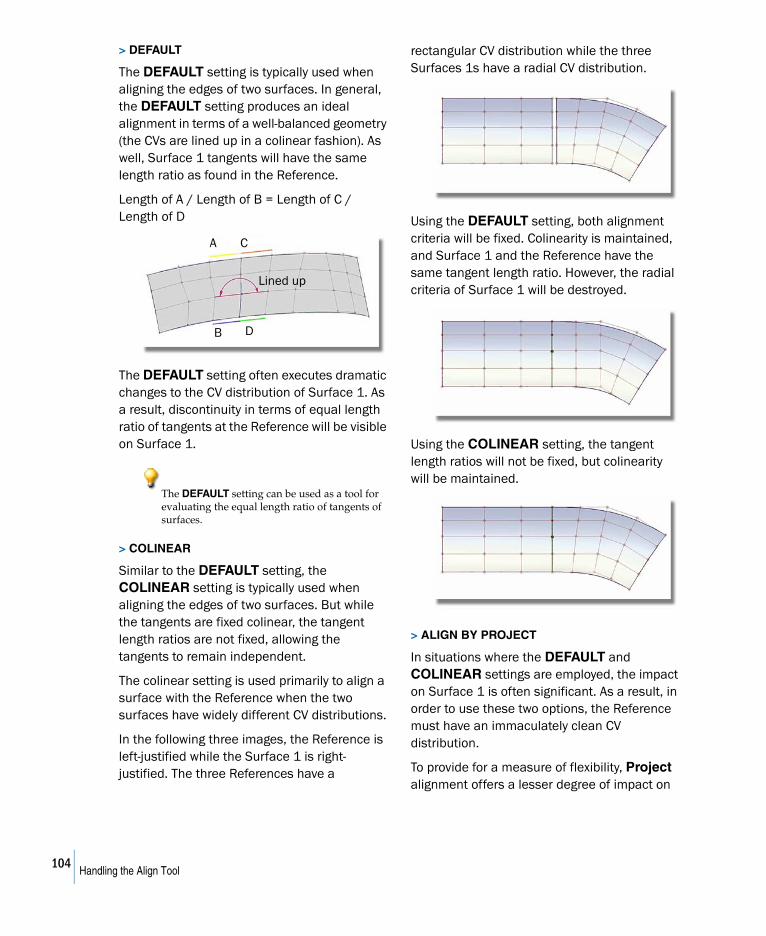
> DEFAULT
The DEFAULT setting is typically used when aligning the edges of two surfaces. In general, the DEFAULT setting produces an ideal alignment in terms of a well-balanced geometry (the CVs are lined up in a colinear fashion). As well, Surface 1 tangents will have the same length ratio as found in the Reference.
Length of A / Length of B = Length of C / Length of D
The DEFAULT setting often executes dramatic changes to the CV distribution of Surface 1. As a result, discontinuity in terms of equal length ratio of tangents at the Reference will be visible on Surface 1.
The DEFAULT setting can be used as a tool for evaluating the equal length ratio of tangents of surfaces.
> COLINEAR
Similar to the DEFAULT setting, the COLINEAR setting is typically used when aligning the edges of two surfaces. But while the tangents are fixed colinear, the tangent length ratios are not fixed, allowing the tangents to remain independent.
The colinear setting is used primarily to align a surface with the Reference when the two surfaces have widely different CV distributions.
In the following three images, the Reference is left-justified while the Surface 1 is right-justified. The three References have a
rectangular CV distribution while the three Surfaces 1s have a radial CV distribution.
Using the DEFAULT setting, both alignment criteria will be fixed. Colinearity is maintained, and Surface 1 and the Reference have the same tangent length ratio. However, the radial criteria of Surface 1 will be destroyed.
Using the COLINEAR setting, the tangent length ratios will not be fixed, but colinearity will be maintained.
> ALIGN BY PROJECT
In situations where the DEFAULT and COLINEAR settings are employed, the impact on Surface 1 is often significant. As a result, in order to use these two options, the Reference must have an immaculately clean CV distribution.
To provide for a measure of flexibility, Project alignment offers a lesser degree of impact on
A C
B D
Lined up
104Handling the Align Tool
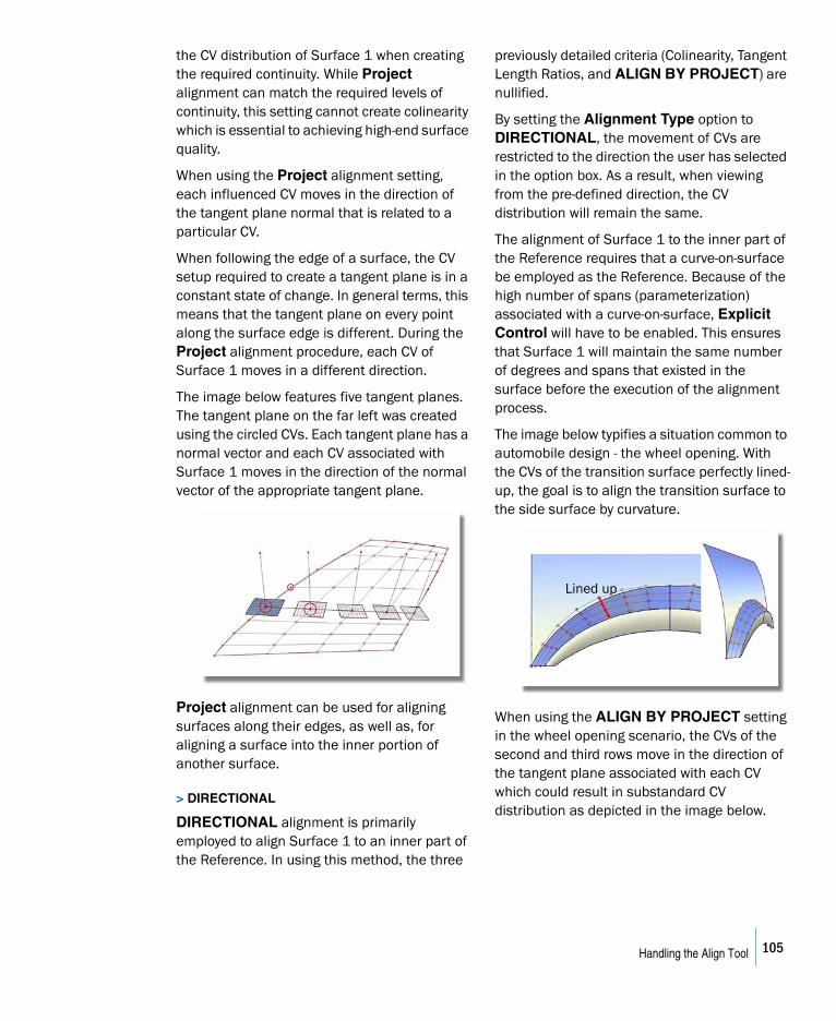
the CV distribution of Surface 1 when creating the required continuity. While Project alignment can match the required levels of continuity, this setting cannot create colinearity which is essential to achieving high-end surface quality.
When using the Project alignment setting, each influenced CV moves in the direction of the tangent plane normal that is related to a particular CV.
When following the edge of a surface, the CV setup required to create a tangent plane is in a constant state of change. In general terms, this means that the tangent plane on every point along the surface edge is different. During the Project alignment procedure, each CV of Surface 1 moves in a different direction.
The image below features five tangent planes. The tangent plane on the far left was created using the circled CVs. Each tangent plane has a normal vector and each CV associated with Surface 1 moves in the direction of the normal vector of the appropriate tangent plane.
Project alignment can be used for aligning surfaces along their edges, as well as, for aligning a surface into the inner portion of another surface.
> DIRECTIONAL
DIRECTIONAL alignment is primarily employed to align Surface 1 to an inner part of the Reference. In using this method, the three
previously detailed criteria (Colinearity, Tangent Length Ratios, and ALIGN BY PROJECT) are nullified.
By setting the Alignment Type option to DIRECTIONAL, the movement of CVs are restricted to the direction the user has selected in the option box. As a result, when viewing from the pre-defined direction, the CV distribution will remain the same.
The alignment of Surface 1 to the inner part of the Reference requires that a curve-on-surface be employed as the Reference. Because of the high number of spans (parameterization) associated with a curve-on-surface, Explicit Control will have to be enabled. This ensures that Surface 1 will maintain the same number of degrees and spans that existed in the surface before the execution of the alignment process.
The image below typifies a situation common to automobile design - the wheel opening. With the CVs of the transition surface perfectly lined-up, the goal is to align the transition surface to the side surface by curvature.
When using the ALIGN BY PROJECT setting in the wheel opening scenario, the CVs of the second and third rows move in the direction of the tangent plane associated with each CV which could result in substandard CV distribution as depicted in the image below.
Lined up
105Handling the Align Tool
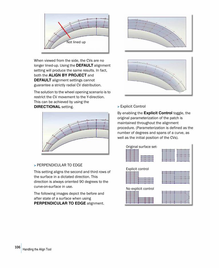
When viewed from the side, the CVs are no longer lined-up. Using the DEFAULT alignment setting will produce the same results. In fact, both the ALIGN BY PROJECT and DEFAULT alignment settings cannot guarantee a strictly radial CV distribution.
The solution to the wheel opening scenario is to restrict the CV movement to the Y-direction. This can be achieved by using the DIRECTIONAL setting.
> PERPENDICULAR TO EDGE
This setting aligns the second and third rows of the surface in a dictated direction. This direction is always oriented 90 degrees to the curve-on-surface in use.
The following images depict the before and after state of a surface when using PERPENDICULAR TO EDGE alignment.
> Explicit Control
By enabling the Explicit Control toggle, the original parameterization of the patch is maintained throughout the alignment procedure. (Parameterization is defined as the number of degrees and spans of a curve, as well as the initial position of the CVs).
Not lined up
Original surface set-
Explicit control
No explicit control
106Handling the Align Tool
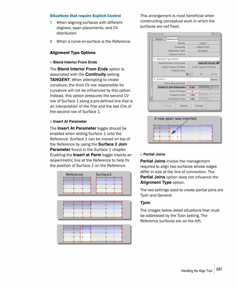
Situations that require Explicit Control
1 When aligning surfaces with different degrees, span placements, and CV distribution
2 When a curve-on-surface is the Reference
Alignment Type Options
> Blend Interior From Ends
The Blend Interior From Ends option is associated with the Continuity setting TANGENT. When attempting to create curvature, the third CV row responsible for curvature will not be influenced by this option. Instead, this option pressures the second CV row of Surface 1 along a pre-defined line that is an interpolation of the first and the last CVs of the second row of Surface 1.
> Insert At Parameter
The Insert At Parameter toggle should be enabled when sliding Surface 1 onto the Reference. Surface 1 can be moved on top of the Reference by using the Surface 2 Join Parameter found in the Surface 1 chapter. Enabling the Insert at Parm toggle inserts an isoperimetric line at the Reference to help fix the position of Surface 1 on the Reference.
This arrangement is most beneficial when constructing conceptual work in which the surfaces are not fixed.
> Partial Joins
Partial Joins involve the management required to align two surfaces whose edges differ in size at the line of connection. The Partial Joins option does not influence the Alignment Type option.
The two settings used to create partial joins are Tjoin and General.
Tjoin
The images below detail situations that must be addressed by the Tjoin setting. The Reference surfaces are on the left.
Reference Surface1
A new span was inserted
107Handling the Align Tool
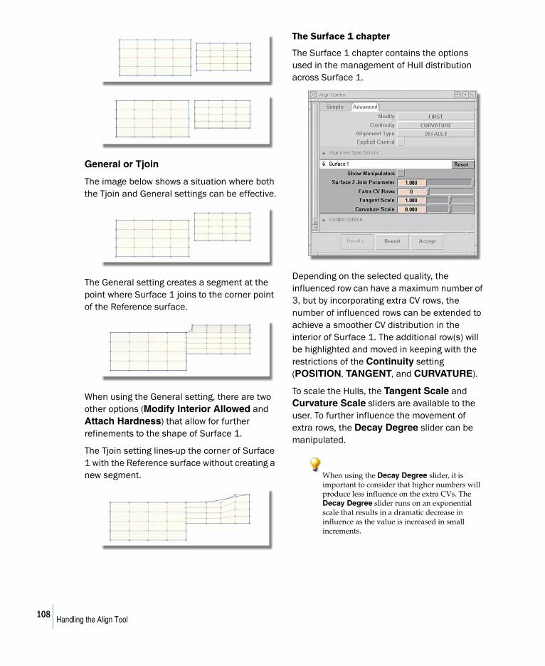
General or Tjoin
The image below shows a situation where both the Tjoin and General settings can be effective.
The General setting creates a segment at the point where Surface 1 joins to the corner point of the Reference surface.
When using the General setting, there are two other options (Modify Interior Allowed and Attach Hardness) that allow for further refinements to the shape of Surface 1.
The Tjoin setting lines-up the corner of Surface 1 with the Reference surface without creating a new segment.
The Surface 1 chapter
The Surface 1 chapter contains the options used in the management of Hull distribution across Surface 1.
Depending on the selected quality, the influenced row can have a maximum number of 3, but by incorporating extra CV rows, the number of influenced rows can be extended to achieve a smoother CV distribution in the interior of Surface 1. The additional row(s) will be highlighted and moved in keeping with the restrictions of the Continuity setting (POSITION, TANGENT, and CURVATURE).
To scale the Hulls, the Tangent Scale and Curvature Scale sliders are available to the user. To further influence the movement of extra rows, the Decay Degree slider can be manipulated.
When using the Decay Degree slider, it is important to consider that higher numbers will produce less influence on the extra CVs. The Decay Degree slider runs on an exponential scale that results in a dramatic decrease in influence as the value is increased in small increments.
108Handling the Align Tool
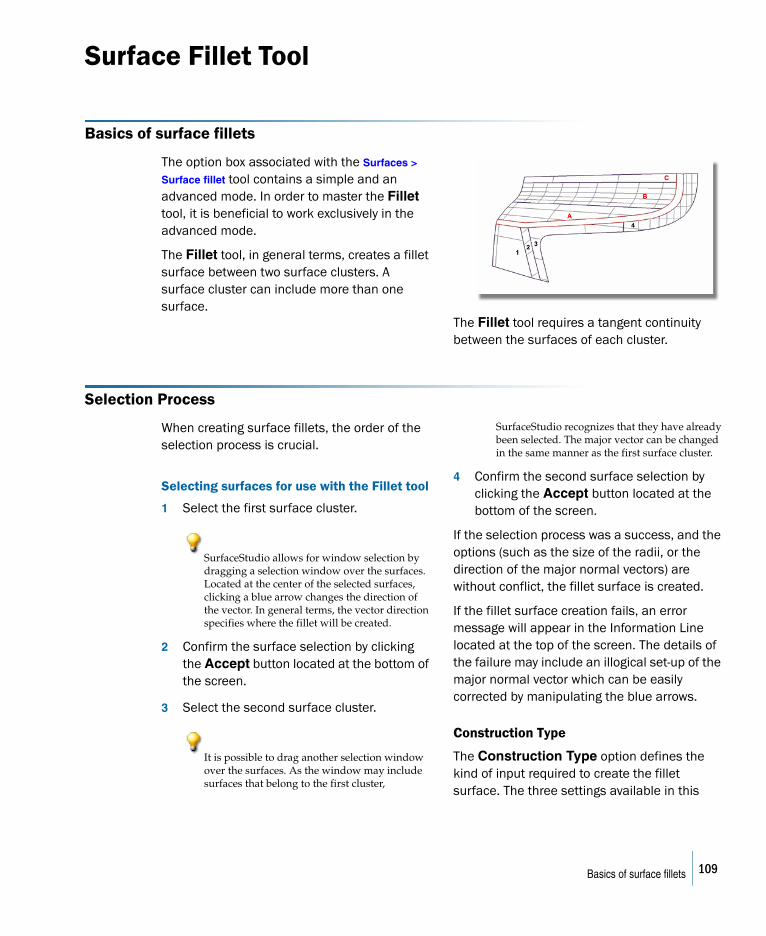
Surface Fillet Tool
Basics of surface fillets
The option box associated with the Surfaces >
Surface fillet tool contains a simple and an advanced mode. In order to master the Fillet tool, it is beneficial to work exclusively in the advanced mode.
The Fillet tool, in general terms, creates a fillet surface between two surface clusters. A surface cluster can include more than one surface.
The Fillet tool requires a tangent continuity between the surfaces of each cluster.
Selection Process
When creating surface fillets, the order of the selection process is crucial.
Selecting surfaces for use with the Fillet tool
1 Select the first surface cluster.
SurfaceStudio allows for window selection by dragging a selection window over the surfaces. Located at the center of the selected surfaces, clicking a blue arrow changes the direction of the vector. In general terms, the vector direction specifies where the fillet will be created.
2 Confirm the surface selection by clicking the Accept button located at the bottom of the screen.
3 Select the second surface cluster.
It is possible to drag another selection window over the surfaces. As the window may include surfaces that belong to the first cluster,
SurfaceStudio recognizes that they have already been selected. The major vector can be changed in the same manner as the first surface cluster.
4 Confirm the second surface selection by clicking the Accept button located at the bottom of the screen.
If the selection process was a success, and the options (such as the size of the radii, or the direction of the major normal vectors) are without conflict, the fillet surface is created.
If the fillet surface creation fails, an error message will appear in the Information Line located at the top of the screen. The details of the failure may include an illogical set-up of the major normal vector which can be easily corrected by manipulating the blue arrows.
Construction Type
The Construction Type option defines the kind of input required to create the fillet surface. The three settings available in this
109Basics of surface fillets
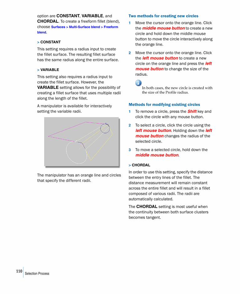
option are CONSTANT, VARIABLE, and CHORDAL. To create a freeform fillet (blend), choose Surfaces > Multi-Surface blend > Freeform
blend.
> CONSTANT
This setting requires a radius input to create the fillet surface. The resulting fillet surface has the same radius along the entire surface.
> VARIABLE
This setting also requires a radius input to create the fillet surface. However, the VARIABLE setting allows for the possibility of creating a fillet surface that uses multiple radii along the length of the fillet.
A manipulator is available for interactively setting the variable radii.
The manipulator has an orange line and circles that specify the different radii.
Two methods for creating new circles
1 Move the cursor onto the orange line. Click the middle mouse button to create a new circle and hold down the middle mouse button to move the circle interactively along the orange line.
2 Move the cursor onto the orange line. Click the left mouse button to create a new circle on the orange line and press the left mouse button to change the size of the radius.
In both cases, the new circle is created with the size of the Profile radius.
Methods for modifying existing circles
1 To remove a circle, press the Shift key and click the circle with any mouse button.
2 To select a circle, click the circle using the left mouse button. Holding down the left mouse button changes the radius of the selected circle.
3 To move a selected circle, hold down the middle mouse button.
> CHORDAL
In order to use this setting, specify the distance between the entry lines of the fillet. The distance measurement will remain constant across the entire fillet and will result in a fillet composed of various radii. The radii are automatically calculated.
The CHORDAL setting is most useful when the continuity between both surface clusters becomes tangent.
110Selection Process
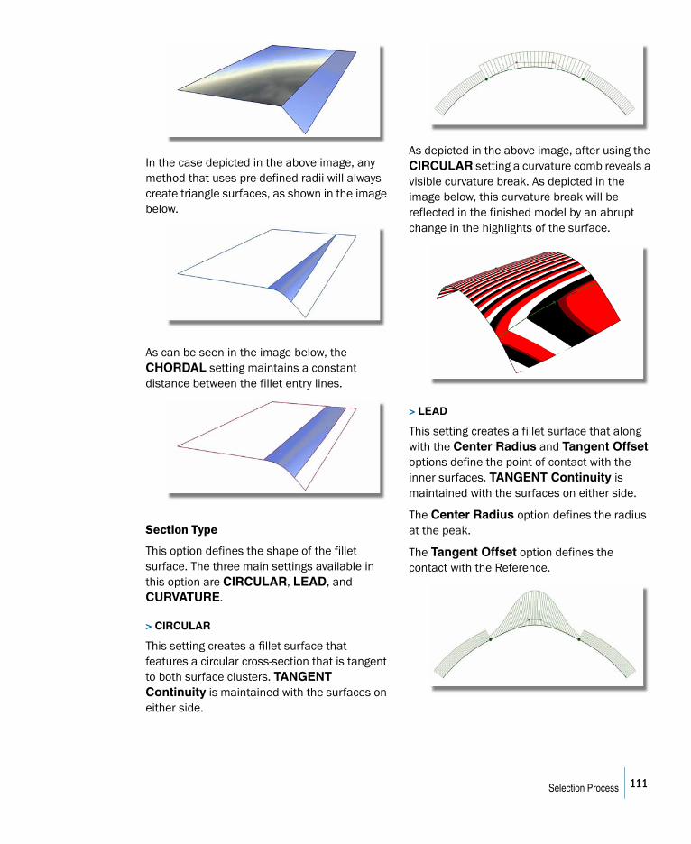
In the case depicted in the above image, any method that uses pre-defined radii will always create triangle surfaces, as shown in the image below.
As can be seen in the image below, the CHORDAL setting maintains a constant distance between the fillet entry lines.
Section Type
This option defines the shape of the fillet surface. The three main settings available in this option are CIRCULAR, LEAD, and CURVATURE.
> CIRCULAR
This setting creates a fillet surface that features a circular cross-section that is tangent to both surface clusters. TANGENT Continuity is maintained with the surfaces on either side.
As depicted in the above image, after using the CIRCULAR setting a curvature comb reveals a visible curvature break. As depicted in the image below, this curvature break will be reflected in the finished model by an abrupt change in the highlights of the surface.
> LEAD
This setting creates a fillet surface that along with the Center Radius and Tangent Offset options define the point of contact with the inner surfaces. TANGENT Continuity is maintained with the surfaces on either side.
The Center Radius option defines the radius at the peak.
The Tangent Offset option defines the contact with the Reference.
111Selection Process
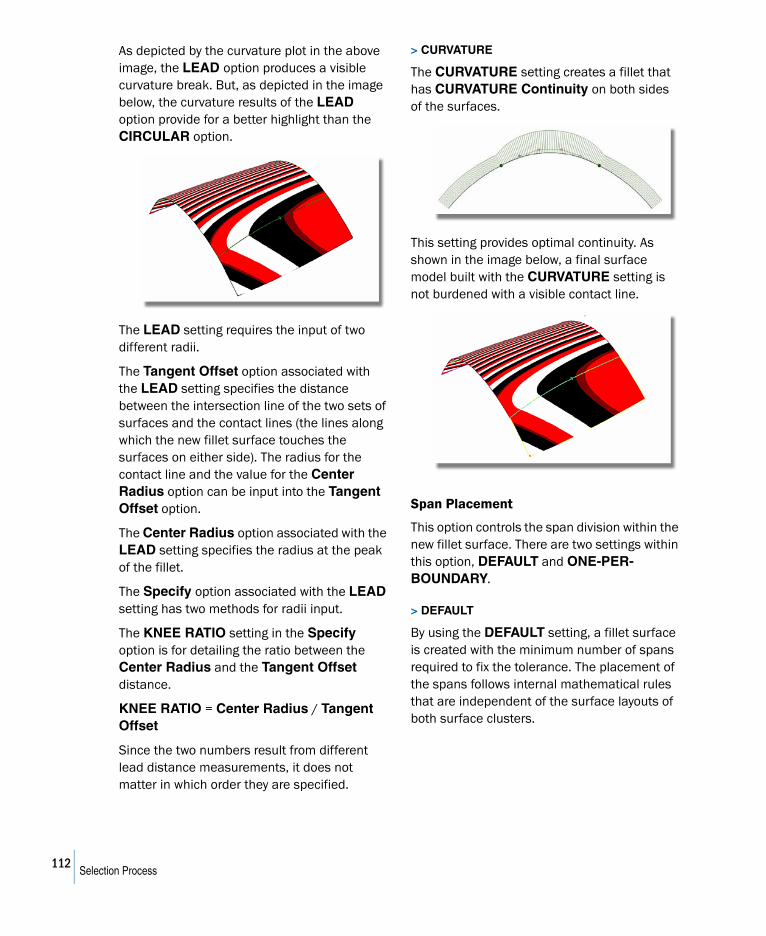
As depicted by the curvature plot in the above image, the LEAD option produces a visible curvature break. But, as depicted in the image below, the curvature results of the LEAD option provide for a better highlight than the CIRCULAR option.
The LEAD setting requires the input of two different radii.
The Tangent Offset option associated with the LEAD setting specifies the distance between the intersection line of the two sets of surfaces and the contact lines (the lines along which the new fillet surface touches the surfaces on either side). The radius for the contact line and the value for the Center Radius option can be input into the Tangent Offset option.
The Center Radius option associated with the LEAD setting specifies the radius at the peak of the fillet.
The Specify option associated with the LEAD setting has two methods for radii input.
The KNEE RATIO setting in the Specify option is for detailing the ratio between the Center Radius and the Tangent Offset distance.
KNEE RATIO = Center Radius / Tangent Offset
Since the two numbers result from different lead distance measurements, it does not matter in which order they are specified.
> CURVATURE
The CURVATURE setting creates a fillet that has CURVATURE Continuity on both sides of the surfaces.
This setting provides optimal continuity. As shown in the image below, a final surface model built with the CURVATURE setting is not burdened with a visible contact line.
Span Placement
This option controls the span division within the new fillet surface. There are two settings within this option, DEFAULT and ONE-PER-BOUNDARY.
> DEFAULT
By using the DEFAULT setting, a fillet surface is created with the minimum number of spans required to fix the tolerance. The placement of the spans follows internal mathematical rules that are independent of the surface layouts of both surface clusters.
112Selection Process
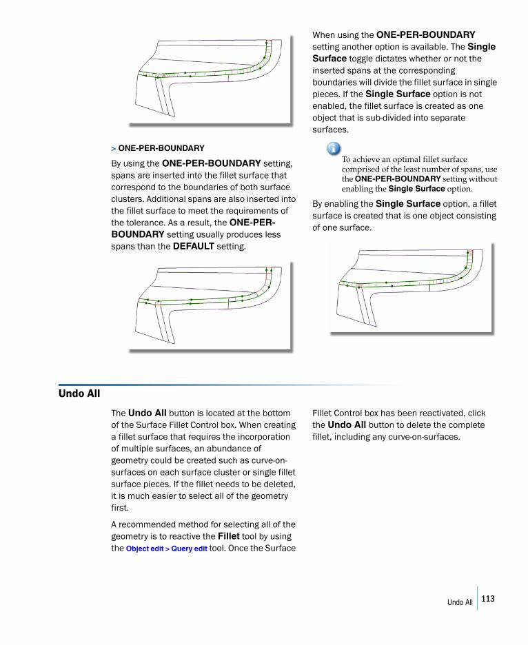
> ONE-PER-BOUNDARY
By using the ONE-PER-BOUNDARY setting, spans are inserted into the fillet surface that correspond to the boundaries of both surface clusters. Additional spans are also inserted into the fillet surface to meet the requirements of the tolerance. As a result, the ONE-PER-BOUNDARY setting usually produces less spans than the DEFAULT setting.
When using the ONE-PER-BOUNDARY setting another option is available. The Single Surface toggle dictates whether or not the inserted spans at the corresponding boundaries will divide the fillet surface in single pieces. If the Single Surface option is not enabled, the fillet surface is created as one object that is sub-divided into separate surfaces.
To achieve an optimal fillet surface comprised of the least number of spans, use the ONE-PER-BOUNDARY setting without enabling the Single Surface option.
By enabling the Single Surface option, a fillet surface is created that is one object consisting of one surface.
Undo All
The Undo All button is located at the bottom of the Surface Fillet Control box. When creating a fillet surface that requires the incorporation of multiple surfaces, an abundance of geometry could be created such as curve-on-surfaces on each surface cluster or single fillet surface pieces. If the fillet needs to be deleted, it is much easier to select all of the geometry first.
A recommended method for selecting all of the geometry is to reactive the Fillet tool by using the Object edit > Query edit tool. Once the Surface
Fillet Control box has been reactivated, click the Undo All button to delete the complete fillet, including any curve-on-surfaces.
113Undo All
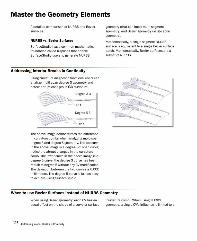
Master the Geometry Elements
A detailed comparison of NURBS and Bezier surfaces.
NURBS vs. Bezier Surfaces
SurfaceStudio has a common mathematical foundation called b-splines that enable SurfaceStudio users to generate NURBS
geometry (that can imply multi segment geometry) and Bezier geometry (single span geometry).
Mathematically, a single segment NURBS surface is equivalent to a single Bezier surface patch. Mathematically, Bezier surfaces are a subset of NURBS.
Addressing Interior Breaks in Continuity
Using curvature diagnostic functions, users can analyze multi-span degree 3 geometry and detect abrupt changes in G3 curvature.
The above image demonstrates the difference in curvature combs when analyzing multi-span degree 3 and degree 5 geometry. The top curve in the above image is a degree 3-3 span curve; notice the abrupt changes in the curvature comb. The lower curve in the above image is a degree 5 curve; the degree 3 curve has been rebuilt to degree 5 without any CV modification. The deviation between the two curves is 0.000 millimeters. The degree 5 curve is just as easy to achieve using SurfaceStudio.
When to use Bezier Surfaces instead of NURBS Geometry
When using Bezier geometry, each CV has an equal effect on the shape of a curve or surface
(curvature comb). When using NURBS geometry, a single CV's influence is limited to a
Degree 3-3
edit
Degree 5-3
edit
114Addressing Interior Breaks in Continuity
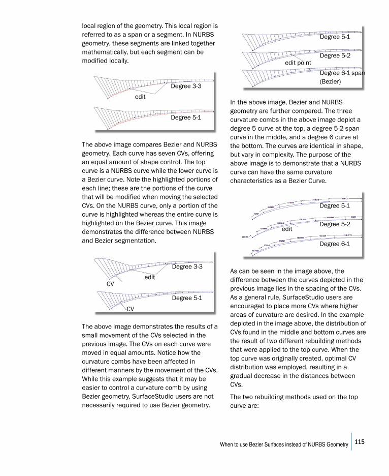
local region of the geometry. This local region is referred to as a span or a segment. In NURBS geometry, these segments are linked together mathematically, but each segment can be modified locally.
The above image compares Bezier and NURBS geometry. Each curve has seven CVs, offering an equal amount of shape control. The top curve is a NURBS curve while the lower curve is a Bezier curve. Note the highlighted portions of each line; these are the portions of the curve that will be modified when moving the selected CVs. On the NURBS curve, only a portion of the curve is highlighted whereas the entire curve is highlighted on the Bezier curve. This image demonstrates the difference between NURBS and Bezier segmentation.
The above image demonstrates the results of a small movement of the CVs selected in the previous image. The CVs on each curve were moved in equal amounts. Notice how the curvature combs have been affected in different manners by the movement of the CVs. While this example suggests that it may be easier to control a curvature comb by using Bezier geometry, SurfaceStudio users are not necessarily required to use Bezier geometry.
In the above image, Bezier and NURBS geometry are further compared. The three curvature combs in the above image depict a degree 5 curve at the top, a degree 5-2 span curve in the middle, and a degree 6 curve at the bottom. The curves are identical in shape, but vary in complexity. The purpose of the above image is to demonstrate that a NURBS curve can have the same curvature characteristics as a Bezier Curve.
As can be seen in the image above, the difference between the curves depicted in the previous image lies in the spacing of the CVs. As a general rule, SurfaceStudio users are encouraged to place more CVs where higher areas of curvature are desired. In the example depicted in the image above, the distribution of CVs found in the middle and bottom curves are the result of two different rebuilding methods that were applied to the top curve. When the top curve was originally created, optimal CV distribution was employed, resulting in a gradual decrease in the distances between CVs.
The two rebuilding methods used on the top curve are:
Degree 3-3
edit
Degree 5-1
CV
CV
Degree 5-1
Degree 3-3
edit
Degree 5-1
Degree 5-2
Degree 6-1 span (Bezier)
edit point
Degree 5-1
Degree 5-2
Degree 6-1
edit
115When to use Bezier Surfaces instead of NURBS Geometry
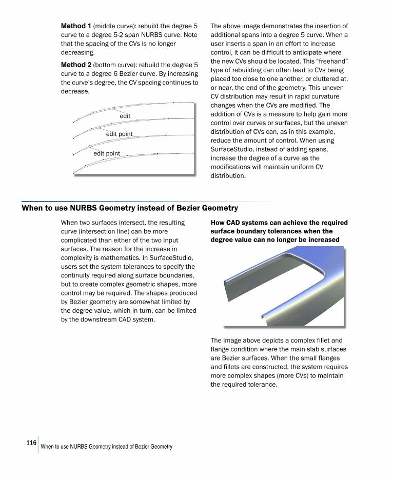
Method 1 (middle curve): rebuild the degree 5 curve to a degree 5-2 span NURBS curve. Note that the spacing of the CVs is no longer decreasing.
Method 2 (bottom curve): rebuild the degree 5 curve to a degree 6 Bezier curve. By increasing the curve's degree, the CV spacing continues to decrease.
The above image demonstrates the insertion of additional spans into a degree 5 curve. When a user inserts a span in an effort to increase control, it can be difficult to anticipate where the new CVs should be located. This “freehand” type of rebuilding can often lead to CVs being placed too close to one another, or cluttered at, or near, the end of the geometry. This uneven CV distribution may result in rapid curvature changes when the CVs are modified. The addition of CVs is a measure to help gain more control over curves or surfaces, but the uneven distribution of CVs can, as in this example, reduce the amount of control. When using SurfaceStudio, instead of adding spans, increase the degree of a curve as the modifications will maintain uniform CV distribution.
When to use NURBS Geometry instead of Bezier Geometry
When two surfaces intersect, the resulting curve (intersection line) can be more complicated than either of the two input surfaces. The reason for the increase in complexity is mathematics. In SurfaceStudio, users set the system tolerances to specify the continuity required along surface boundaries, but to create complex geometric shapes, more control may be required. The shapes produced by Bezier geometry are somewhat limited by the degree value, which in turn, can be limited by the downstream CAD system.
How CAD systems can achieve the required surface boundary tolerances when the degree value can no longer be increased
The image above depicts a complex fillet and flange condition where the main slab surfaces are Bezier surfaces. When the small flanges and fillets are constructed, the system requires more complex shapes (more CVs) to maintain the required tolerance.
edit
edit point
edit point
116When to use NURBS Geometry instead of Bezier Geometry
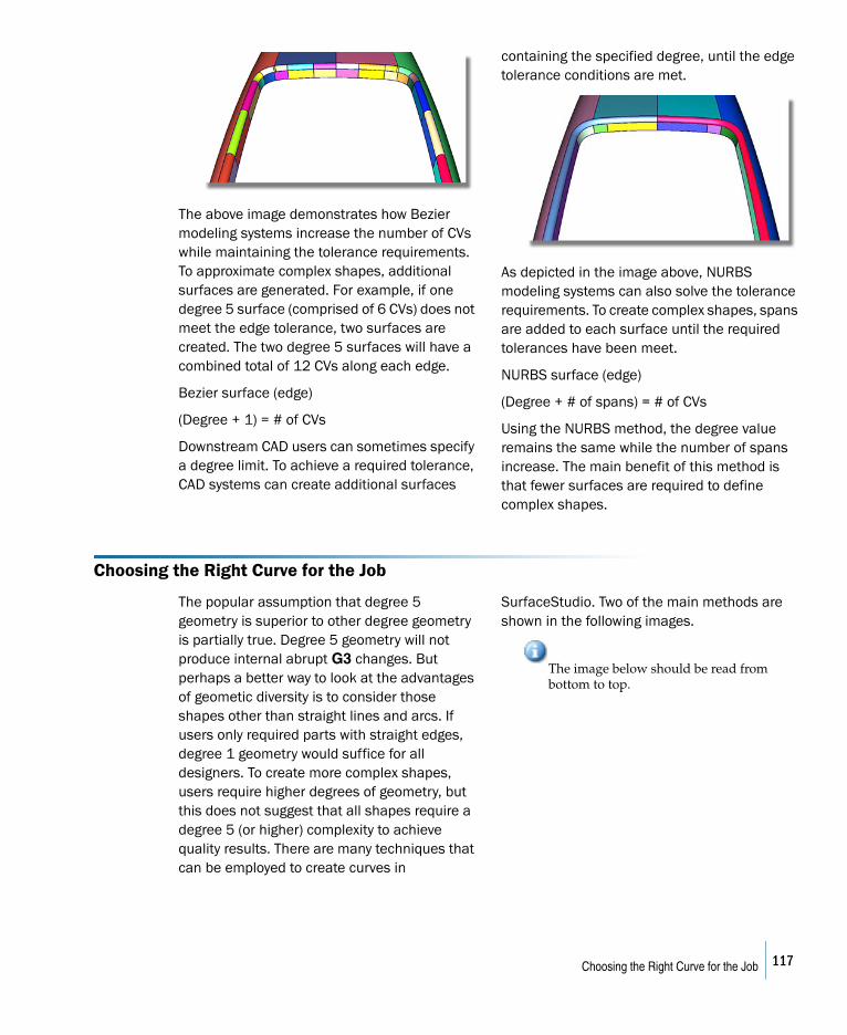
The above image demonstrates how Bezier modeling systems increase the number of CVs while maintaining the tolerance requirements. To approximate complex shapes, additional surfaces are generated. For example, if one degree 5 surface (comprised of 6 CVs) does not meet the edge tolerance, two surfaces are created. The two degree 5 surfaces will have a combined total of 12 CVs along each edge.
Bezier surface (edge)
(Degree + 1) = # of CVs
Downstream CAD users can sometimes specify a degree limit. To achieve a required tolerance, CAD systems can create additional surfaces
containing the specified degree, until the edge tolerance conditions are met.
As depicted in the image above, NURBS modeling systems can also solve the tolerance requirements. To create complex shapes, spans are added to each surface until the required tolerances have been meet.
NURBS surface (edge)
(Degree + # of spans) = # of CVs
Using the NURBS method, the degree value remains the same while the number of spans increase. The main benefit of this method is that fewer surfaces are required to define complex shapes.
Choosing the Right Curve for the Job
The popular assumption that degree 5 geometry is superior to other degree geometry is partially true. Degree 5 geometry will not produce internal abrupt G3 changes. But perhaps a better way to look at the advantages of geometic diversity is to consider those shapes other than straight lines and arcs. If users only required parts with straight edges, degree 1 geometry would suffice for all designers. To create more complex shapes, users require higher degrees of geometry, but this does not suggest that all shapes require a degree 5 (or higher) complexity to achieve quality results. There are many techniques that can be employed to create curves in
SurfaceStudio. Two of the main methods are shown in the following images.
The image below should be read from bottom to top.
117Choosing the Right Curve for the Job
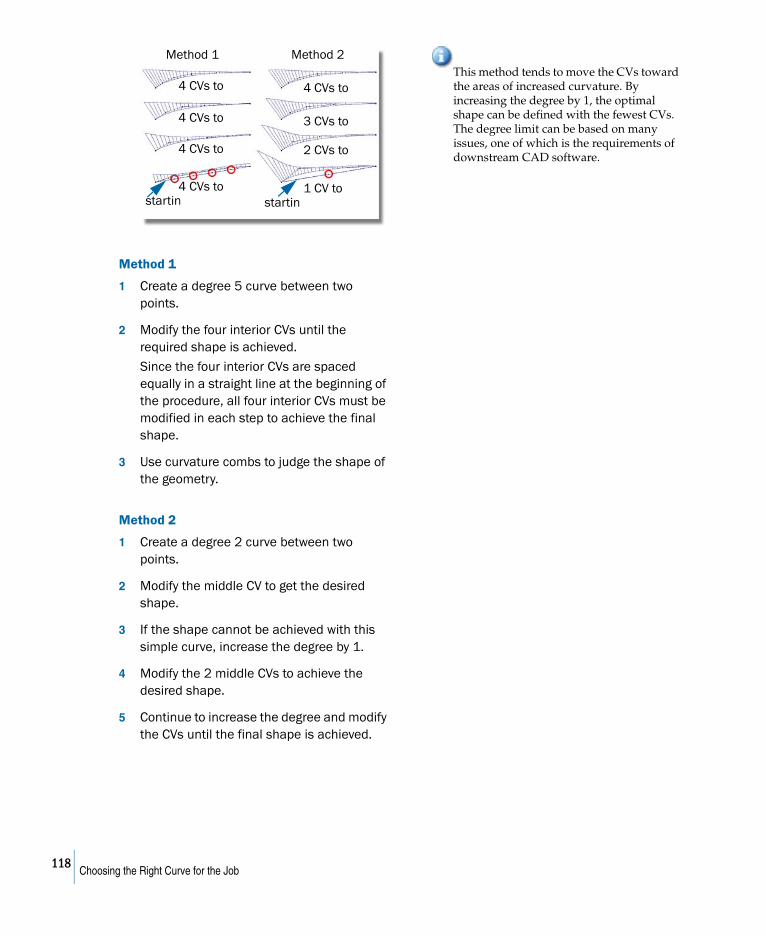
Method 1
1 Create a degree 5 curve between two points.
2 Modify the four interior CVs until the required shape is achieved.
Since the four interior CVs are spaced equally in a straight line at the beginning of the procedure, all four interior CVs must be modified in each step to achieve the final shape.
3 Use curvature combs to judge the shape of the geometry.
Method 2
1 Create a degree 2 curve between two points.
2 Modify the middle CV to get the desired shape.
3 If the shape cannot be achieved with this simple curve, increase the degree by 1.
4 Modify the 2 middle CVs to achieve the desired shape.
5 Continue to increase the degree and modify the CVs until the final shape is achieved.
This method tends to move the CVs toward the areas of increased curvature. By increasing the degree by 1, the optimal shape can be defined with the fewest CVs. The degree limit can be based on many issues, one of which is the requirements of downstream CAD software.
Method 1 Method 2
startin startin4 CVs to
4 CVs to
4 CVs to
4 CVs to 4 CVs to
3 CVs to
2 CVs to
1 CV to
118Choosing the Right Curve for the Job
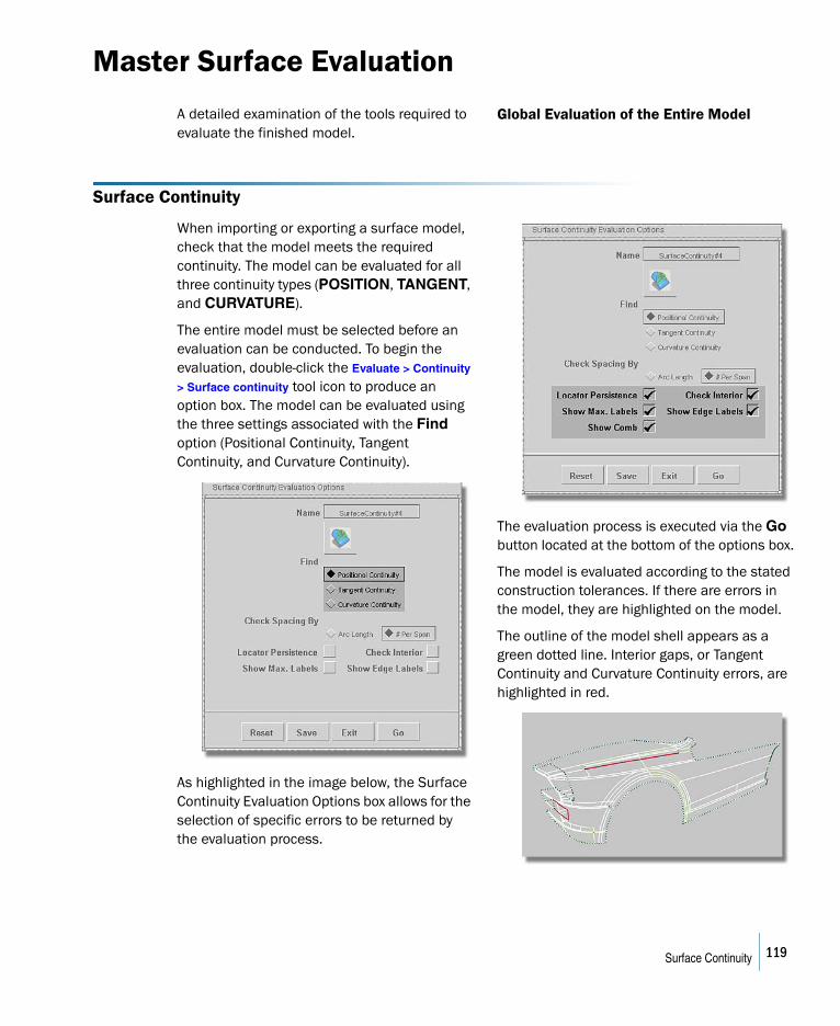
Master Surface Evaluation
A detailed examination of the tools required to evaluate the finished model.
Global Evaluation of the Entire Model
Surface Continuity
When importing or exporting a surface model, check that the model meets the required continuity. The model can be evaluated for all three continuity types (POSITION, TANGENT, and CURVATURE).
The entire model must be selected before an evaluation can be conducted. To begin the evaluation, double-click the Evaluate > Continuity
> Surface continuity tool icon to produce an option box. The model can be evaluated using the three settings associated with the Find option (Positional Continuity, Tangent Continuity, and Curvature Continuity).
As highlighted in the image below, the Surface Continuity Evaluation Options box allows for the selection of specific errors to be returned by the evaluation process.
The evaluation process is executed via the Go button located at the bottom of the options box.
The model is evaluated according to the stated construction tolerances. If there are errors in the model, they are highlighted on the model.
The outline of the model shell appears as a green dotted line. Interior gaps, or Tangent Continuity and Curvature Continuity errors, are highlighted in red.
119Surface Continuity
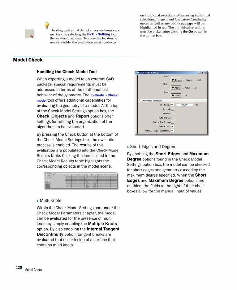
The diagnostics that depict errors are temporary markers. By selecting the Pick > Nothing tool, the locators disappear. To allow the locators to remain visible, the evaluation must conducted
on individual selections. When using individual selections, Tangent and Curvature Continuity errors as well as any additional gaps will be highlighted in red. The individual selections must be picked after clicking the Go button in the option box.
Model Check
Handling the Check Model Tool
When exporting a model to an external CAD package, special requirements must be addressed in terms of the mathematical behavior of the geometry. The Evaluate > Check
model tool offers additional capabilities for evaluating the geometry of a model. At the top of the Check Model Settings option box, the Check, Objects and Report options offer settings for refining the organization of the algorithms to be evaluated.
By pressing the Check button at the bottom of the Check Model Settings box, the evaluation process is enabled. The results of this evaluation are populated into the Check Model Results table. Clicking the items listed in the Check Model Results table highlights the corresponding objects in the model scene.
> Multi Knots
Within the Check Model Settings box, under the Check Model Parameters chapter, the model can be evaluated for the presence of multi knots by simply enabling the Multiple Knots option. By also enabling the Internal Tangent Discontinuity option, tangent breaks are evaluated that occur inside of a surface that contains multi knots.
> Short Edges and Degree
By enabling the Short Edges and Maximum Degree options found in the Check Model Settings option box, the model can be checked for short edges and geometry exceeding the maximum degree specified. When the Short Edges and Maximum Degree options are enabled, the fields to the right of their check boxes allow for the manual input of values.
120Model Check
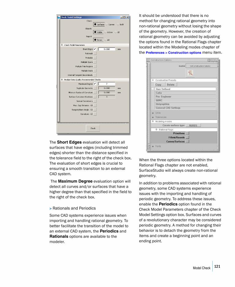
The Short Edges evaluation will detect all surfaces that have edges (including trimmed edges) shorter than the distance specified in the tolerance field to the right of the check box. The evaluation of short edges is crucial to ensuring a smooth transition to an external CAD system.
The Maximum Degree evaluation option will detect all curves and/or surfaces that have a higher degree than that specified in the field to the right of the check box.
> Rationals and Periodics
Some CAD systems experience issues when importing and handling rational geometry. To better facilitate the transition of the model to an external CAD system, the Periodics and Rationals options are available to the modeler.
It should be understood that there is no method for changing rational geometry into non-rational geometry without losing the shape of the geometry. However, the creation of rational geometry can be avoided by adjusting the options found in the Rational Flags chapter located within the Modeling modes chapter of the Preferences > Construction options menu item.
When the three options located within the Rational Flags chapter are not enabled, SurfaceStudio will always create non-rational geometry.
In addition to problems associated with rational geometry, some CAD systems experience issues with the importing and handling of periodic geometry. To address these issues, enable the Periodics option found in the Check Model Parameters chapter of the Check Model Settings option box. Surfaces and curves of a revolutionary character may be considered periodic geometry. A method for changing their behavior is to detach the geometry from the items and create a beginning point and an ending point.
121Model Check
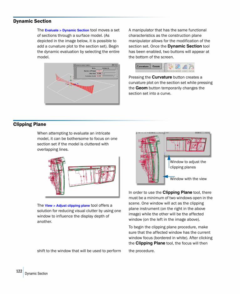
Dynamic Section
The Evaluate > Dynamic Section tool moves a set of sections through a surface model. (As depicted in the image below, it is possible to add a curvature plot to the section set). Begin the dynamic evaluation by selecting the entire model.
A manipulator that has the same functional characteristics as the construction plane manipulator allows for the modification of the section set. Once the Dynamic Section tool has been enabled, two buttons will appear at the bottom of the screen.
Pressing the Curvature button creates a curvature plot on the section set while pressing the Geom button temporarily changes the section set into a curve.
Clipping Plane
When attempting to evaluate an intricate model, it can be bothersome to focus on one section set if the model is cluttered with overlapping lines.
The View > Adjust clipping plane tool offers a solution for reducing visual clutter by using one window to influence the display depth of another.
In order to use the Clipping Plane tool, there must be a minimum of two windows open in the scene. One window will act as the clipping plane instrument (on the right in the above image) while the other will be the affected window (on the left in the image above).
To begin the clipping plane procedure, make sure that the affected window has the current window focus (bordered in white). After clicking the Clipping Plane tool, the focus will then
shift to the window that will be used to perform the procedure.
Window with the view
Window to adjust the clipping planes
122Dynamic Section
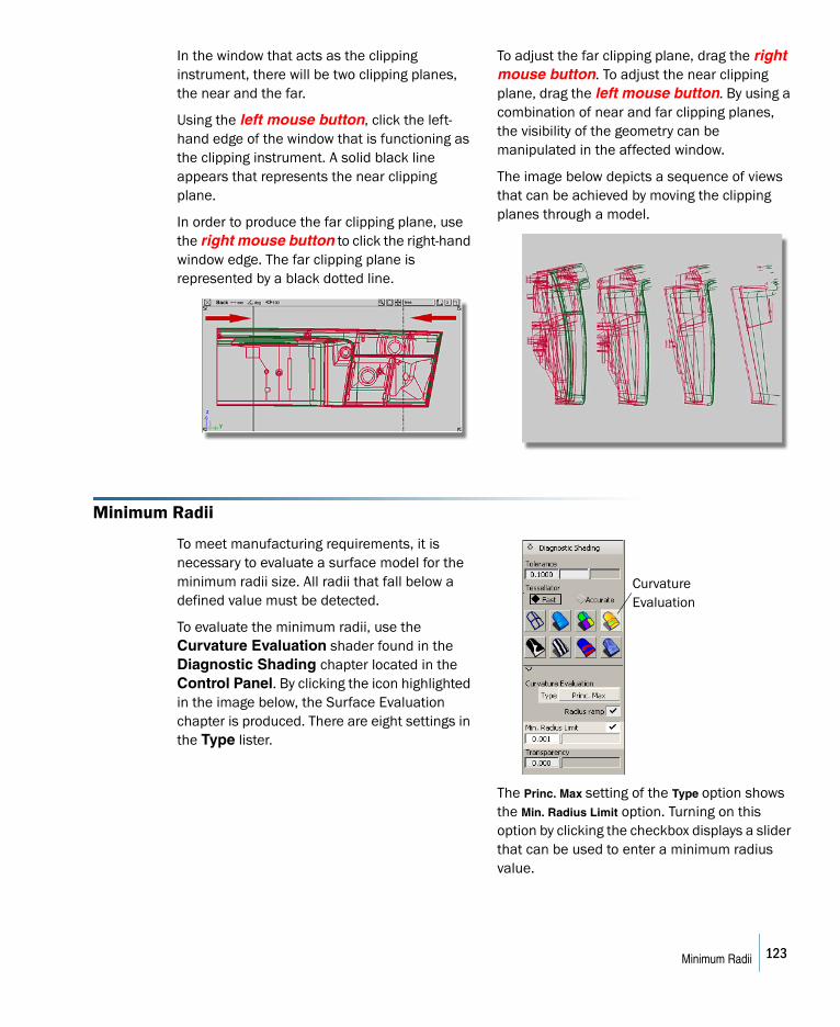
In the window that acts as the clipping instrument, there will be two clipping planes, the near and the far.
Using the left mouse button, click the left-hand edge of the window that is functioning as the clipping instrument. A solid black line appears that represents the near clipping plane.
In order to produce the far clipping plane, use the right mouse button to click the right-hand window edge. The far clipping plane is represented by a black dotted line.
To adjust the far clipping plane, drag the right mouse button. To adjust the near clipping plane, drag the left mouse button. By using a combination of near and far clipping planes, the visibility of the geometry can be manipulated in the affected window.
The image below depicts a sequence of views that can be achieved by moving the clipping planes through a model.
Minimum Radii
To meet manufacturing requirements, it is necessary to evaluate a surface model for the minimum radii size. All radii that fall below a defined value must be detected.
To evaluate the minimum radii, use the Curvature Evaluation shader found in the Diagnostic Shading chapter located in the Control Panel. By clicking the icon highlighted in the image below, the Surface Evaluation chapter is produced. There are eight settings in the Type lister.
The Princ. Max setting of the Type option shows the Min. Radius Limit option. Turning on this option by clicking the checkbox displays a slider that can be used to enter a minimum radius value.
Curvature Evaluation
123Minimum Radii
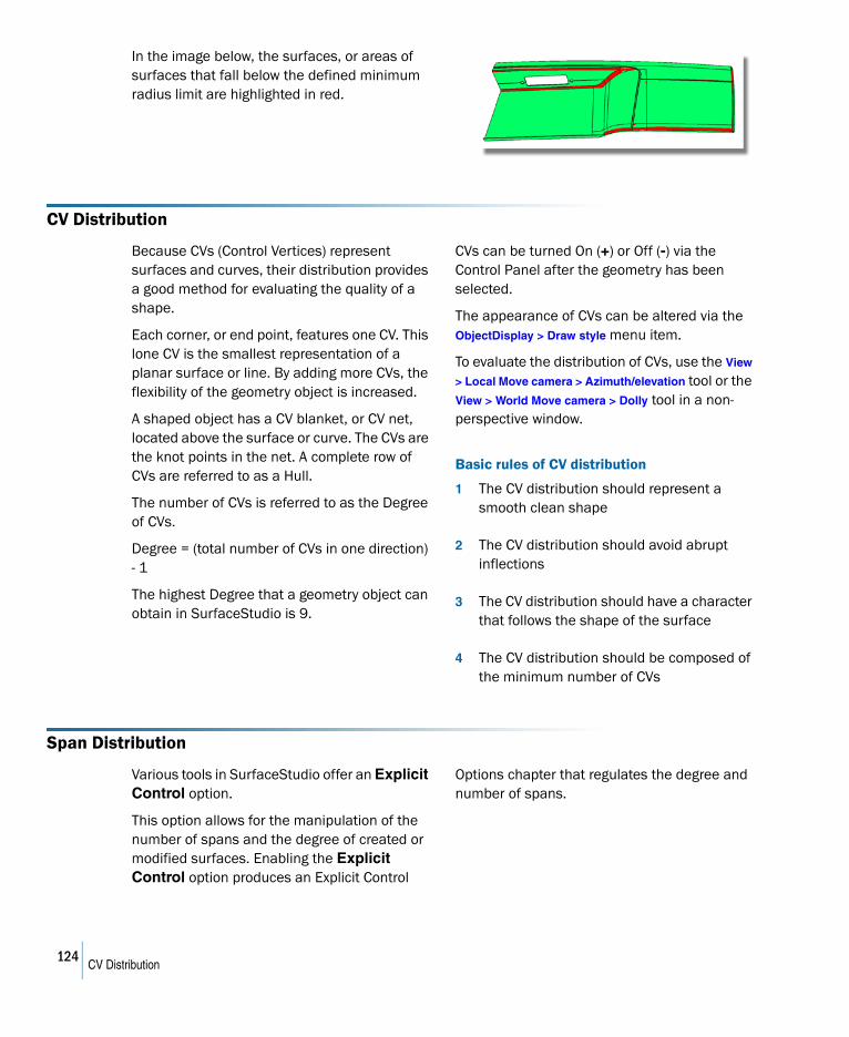
In the image below, the surfaces, or areas of surfaces that fall below the defined minimum radius limit are highlighted in red.
CV Distribution
Because CVs (Control Vertices) represent surfaces and curves, their distribution provides a good method for evaluating the quality of a shape.
Each corner, or end point, features one CV. This lone CV is the smallest representation of a planar surface or line. By adding more CVs, the flexibility of the geometry object is increased.
A shaped object has a CV blanket, or CV net, located above the surface or curve. The CVs are the knot points in the net. A complete row of CVs are referred to as a Hull.
The number of CVs is referred to as the Degree of CVs.
Degree = (total number of CVs in one direction) - 1
The highest Degree that a geometry object can obtain in SurfaceStudio is 9.
CVs can be turned On (+) or Off (-) via the Control Panel after the geometry has been selected.
The appearance of CVs can be altered via the ObjectDisplay > Draw style menu item.
To evaluate the distribution of CVs, use the View
> Local Move camera > Azimuth/elevation tool or the View > World Move camera > Dolly tool in a non-perspective window.
Basic rules of CV distribution
1 The CV distribution should represent a smooth clean shape
2 The CV distribution should avoid abrupt inflections
3 The CV distribution should have a character that follows the shape of the surface
4 The CV distribution should be composed of the minimum number of CVs
Span Distribution
Various tools in SurfaceStudio offer an Explicit Control option.
This option allows for the manipulation of the number of spans and the degree of created or modified surfaces. Enabling the Explicit Control option produces an Explicit Control
Options chapter that regulates the degree and number of spans.
124CV Distribution
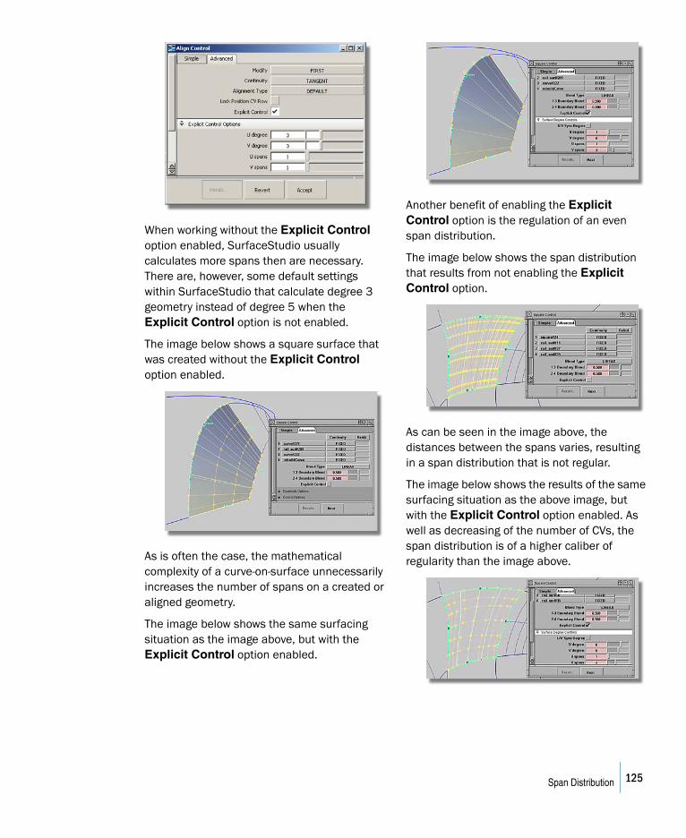
When working without the Explicit Control option enabled, SurfaceStudio usually calculates more spans then are necessary. There are, however, some default settings within SurfaceStudio that calculate degree 3 geometry instead of degree 5 when the Explicit Control option is not enabled.
The image below shows a square surface that was created without the Explicit Control option enabled.
As is often the case, the mathematical complexity of a curve-on-surface unnecessarily increases the number of spans on a created or aligned geometry.
The image below shows the same surfacing situation as the image above, but with the Explicit Control option enabled.
Another benefit of enabling the Explicit Control option is the regulation of an even span distribution.
The image below shows the span distribution that results from not enabling the Explicit Control option.
As can be seen in the image above, the distances between the spans varies, resulting in a span distribution that is not regular.
The image below shows the results of the same surfacing situation as the above image, but with the Explicit Control option enabled. As well as decreasing of the number of CVs, the span distribution is of a higher caliber of regularity than the image above.
125Span Distribution
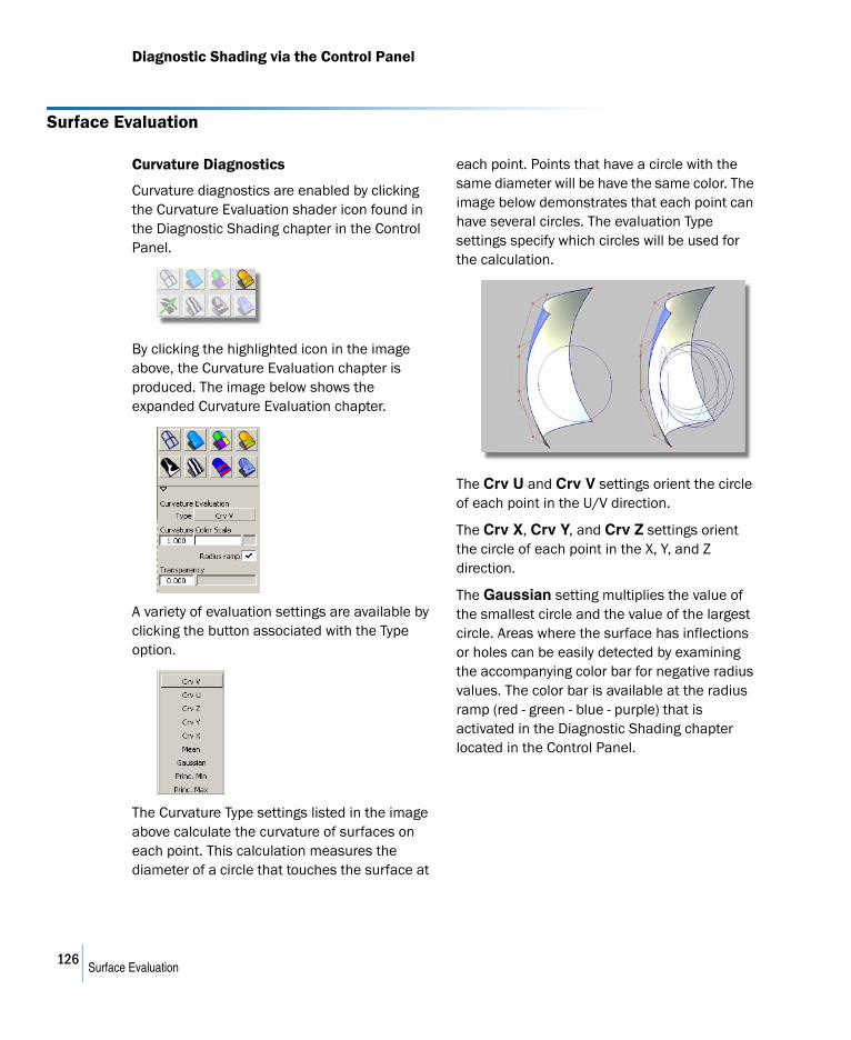
Diagnostic Shading via the Control Panel
Surface Evaluation
Curvature Diagnostics
Curvature diagnostics are enabled by clicking the Curvature Evaluation shader icon found in the Diagnostic Shading chapter in the Control Panel.
By clicking the highlighted icon in the image above, the Curvature Evaluation chapter is produced. The image below shows the expanded Curvature Evaluation chapter.
A variety of evaluation settings are available by clicking the button associated with the Type option.
The Curvature Type settings listed in the image above calculate the curvature of surfaces on each point. This calculation measures the diameter of a circle that touches the surface at
each point. Points that have a circle with the same diameter will be have the same color. The image below demonstrates that each point can have several circles. The evaluation Type settings specify which circles will be used for the calculation.
The Crv U and Crv V settings orient the circle of each point in the U/V direction.
The Crv X, Crv Y, and Crv Z settings orient the circle of each point in the X, Y, and Z direction.
The Gaussian setting multiplies the value of the smallest circle and the value of the largest circle. Areas where the surface has inflections or holes can be easily detected by examining the accompanying color bar for negative radius values. The color bar is available at the radius ramp (red - green - blue - purple) that is activated in the Diagnostic Shading chapter located in the Control Panel.
126Surface Evaluation
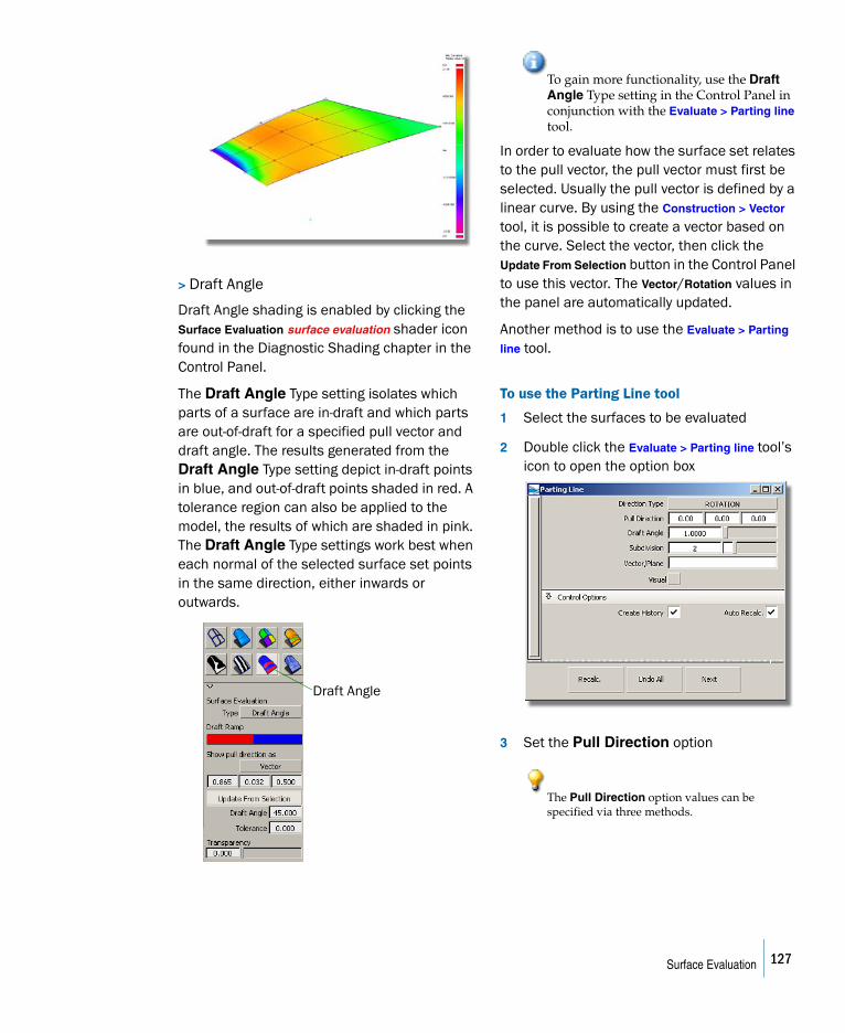
> Draft Angle
Draft Angle shading is enabled by clicking the Surface Evaluation surface evaluation shader icon found in the Diagnostic Shading chapter in the Control Panel.
The Draft Angle Type setting isolates which parts of a surface are in-draft and which parts are out-of-draft for a specified pull vector and draft angle. The results generated from the Draft Angle Type setting depict in-draft points in blue, and out-of-draft points shaded in red. A tolerance region can also be applied to the model, the results of which are shaded in pink. The Draft Angle Type settings work best when each normal of the selected surface set points in the same direction, either inwards or outwards.
To gain more functionality, use the Draft Angle Type setting in the Control Panel in conjunction with the Evaluate > Parting line tool.
In order to evaluate how the surface set relates to the pull vector, the pull vector must first be selected. Usually the pull vector is defined by a linear curve. By using the Construction > Vector tool, it is possible to create a vector based on the curve. Select the vector, then click the Update From Selection button in the Control Panel to use this vector. The Vector/Rotation values in the panel are automatically updated.
Another method is to use the Evaluate > Parting
line tool.
To use the Parting Line tool
1 Select the surfaces to be evaluated
2 Double click the Evaluate > Parting line tool’s icon to open the option box
3 Set the Pull Direction option
The Pull Direction option values can be specified via three methods.
Draft Angle
127Surface Evaluation
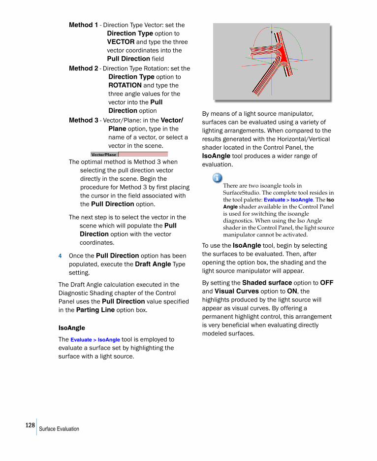
Method 1 - Direction Type Vector: set the Direction Type option to VECTOR and type the three vector coordinates into the Pull Direction field
Method 2 - Direction Type Rotation: set the Direction Type option to ROTATION and type the three angle values for the vector into the Pull Direction option
Method 3 - Vector/Plane: in the Vector/Plane option, type in the name of a vector, or select a vector in the scene.
The optimal method is Method 3 when selecting the pull direction vector directly in the scene. Begin the procedure for Method 3 by first placing the cursor in the field associated with the Pull Direction option.
The next step is to select the vector in the scene which will populate the Pull Direction option with the vector coordinates.
4 Once the Pull Direction option has been populated, execute the Draft Angle Type setting.
The Draft Angle calculation executed in the Diagnostic Shading chapter of the Control Panel uses the Pull Direction value specified in the Parting Line option box.
IsoAngle
The Evaluate > IsoAngle tool is employed to evaluate a surface set by highlighting the surface with a light source.
By means of a light source manipulator, surfaces can be evaluated using a variety of lighting arrangements. When compared to the results generated with the Horizontal/Vertical shader located in the Control Panel, the IsoAngle tool produces a wider range of evaluation.
There are two isoangle tools in SurfaceStudio. The complete tool resides in the tool palette: Evaluate > IsoAngle. The Iso Angle shader available in the Control Panel is used for switching the isoangle diagnostics. When using the Iso Angle shader in the Control Panel, the light source manipulator cannot be activated.
To use the IsoAngle tool, begin by selecting the surfaces to be evaluated. Then, after opening the option box, the shading and the light source manipulator will appear.
By setting the Shaded surface option to OFF and Visual Curves option to ON, the highlights produced by the light source will appear as visual curves. By offering a permanent highlight control, this arrangement is very beneficial when evaluating directly modeled surfaces.
128Surface Evaluation
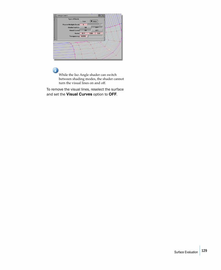
While the Iso Angle shader can switch between shading modes, the shader cannot turn the visual lines on and off.
To remove the visual lines, reselect the surface and set the Visual Curves option to OFF.
129Surface Evaluation

130Surface Evaluation

Numerics3D model
changing view 25–32
Aactive window 8adding
bookmarks 31adjusting
rail surfaces 99theoretical line 81transition surfaces 107
Alias|WavefrontSpider 40
Align toolAlignment Type Option 87constructing a new construction history 87
alignmentaligning two curves 64construction history 116curve on surfaces 115surfaces 115Z-scan lines. 62
Angle optionDraft tool 69
applicationstarting up 2
arranging windows 5, 8arrow on tool icons 10assigning
Layers 101Auto Align at Surface Corners option 123axis
manipulators 111
Bball corners 110
creating 111CV modification 116direct modeling 114guidelines 110position continuity 115
Bezier Surfaces 146Bezier surfaces 111Blend constraint G2 53Blend curve create tool
Auto Align at Surface Corners option 123Knot Spacing option 123
blend curves 51, 54between surfaces and fillets 98blend points 52changing continuity types 53compared to edit point curves 64curvature combs 103direct modeling 105modifying 93modifying to fit to surfaces 99position continuity 92theoretical line 73transition surfaces 92, 102using 52
blend pointdisplay 122placement 122
blend points 52
information on 52locators 93
BlendCrv ToolsBlend curve create 52Blend curve edit tangent 55Constraint Continuity 53manipulators 55
bookmarksadding 31, 32removing 32renaming 32setting and showing 31using 32
CCAD systems 148calculations
reactivate 94suspend 94suspend rebuilds 94
cameramoving 25–32tracking, dollying and tumbling 25
camera move keys 26camera move mode 25center line 49
creating 49developing surfaces 68establishing 49isolating 49sketching 45
Center pivot tool 61changing view
Look at tool 27Viewing Panel 29
click viiiClipping Plane tool 154closing windows 6comb scale
changing values 56components 35concave 71cone 11Connection 126construction history
Align tool 87alignment 116construction plane 89surfaces 81
construction planeconstruction history 89intersecting with a surface 90NURBS 90using 89
construction tolerances 40solid modeling systems 40
Construction Typecollar 68flange 68
Construction Vector tool 159Continuity 127
Interior Breaks 146continuity 53
changing blend curve types 53
163

curvature 56, 65curvature G2 53, 56defined 53position G0 53, 65tangent G1 53, 65types 53values 53
Control Panel 43Cross section tool 69, 90loading shelves 43location 4Move CV tool 57Step size value 84
conventionsgraphic viii
convex 71correcting
curvature combs 103courseware
installing 1CourseWare directory 42creating
ball corners 111curvature combs 103fillet surfaces 85rail surface 95square surfaces 104
Cross section tool 69, 90Crv U setting 159Crv V setting 159Crv X setting 159Crv Y setting 159Crv Z setting 159Curvature button 154curvature combs
blend curves 103correcting 103creating 103duplicated curve 103modifying 103optimal state 57
curvature connectionrestoring 116
curvature continuity 53, 65Curvature Diagnostics 158Curvature type
Geometric setting 127Parametric setting 127
Curve curvature tool 103Curve Edit
Curve planarize tool 72curve on surfaces
alignment 115fillet surfaces 90isoperimetric directions 90Query Edit tool 104Trim Type option 119trimming 119
curve snapping 92Curves
Fit Curve tool 50New Curve tools 60
curvesaligning two curves 64
checking curvature 56, 62correcting 97curve snapping 65, 92cutting curves using reference geometry 92direct modeling 57, 65extending 77fitting across the Y0 plane 59increasing CVs 61patch layouts 103planarizing 72snapping to a pre-defined point 104surfaces 103tips for edit points 64undo extensions 78using edit point curves 63
customizinghot keys 23marking menus 21, 22shelves 16–21
CV distribution 51, 106modification method 1 54modification method 2 54NURBS 90Rebuild option 109
CV modificationball corners 116fitting transition surfaces 106manipulators 56
CV/Hull option 51CVs
increasing 61Move CV tool 57moving in non-proportional scale 61moving in the Z-direction 61selecting 106
cylinder 12
DDAG, see directed acyclic graphdata input types
completed model modification 40sketches & packages 40sorted data 40surface modeling 40
Degreetextbox 61
degreeedit point curves 83increasing 79, 106maximum number of CVs 107
DeleteDelete all locators 57
devaitionbetween surfaces and scan lines 84
direct modelingball corners 114blend curves 105curves 57, 65surfaces 70
Direction setting 125Direction Type option 160directory
wire files 41Display
164

blend points 122Display shelf 51distribution
CV 51Hull 51
dollying 25double-click viiidraft
surfaces 78Draft Angle setting 159Draft tool
Angle option 69creating new surfaces 69
drag ixduplicated curve
curvature combs 103Dynamic Section tool 154
Eedges
shaping 97Edit
Duplicate 60edit point curves
compared to blend curves 64degree 3 83increasing degree value 83new curves 60tips 64using 63
edit tangent 55manipulators 55
EvaluateIsoAngle tool 113
Explicit Control 112, 157extending
curves 77theoretical line 77
Ffiles
opening 41, 42organizating 41wire 41
fillet surfacesblend curves 98creating 85curve on surfaces 90isoperimetric curves 101Radius option 85
flange 68from 86
GG0 53, 65G1 53, 65G2 53, 65G3
Internal Abrupt Changes 149Gausssian setting 159Geom button 154Geometric curvature type 123Geometric setting 127geometry
cutting curves 92
Geometry optionNURBS 90
Geometry setting 125graphic conventions viiigrid snapping 11
see also hot keys 10
Hhelp menu 5Hide Unselected Objects menu item 50
Auto Load option 50Load option 50Unload option 50
historyconstruction history 81
hot keys 16, 23camera move keys 26camera move mode 25customizing 23Viewing Panel 102
Hullchanging the theoretical line 86distribution 51
Iicon size
interface options 20icons
Viewing Panel 63increasing
degree values 79, 106Information Window 124installation
courseware 1interface
control panel 4main window 4menu bar 4overview 4palette 4shelves 4
interface optionsicon size 20point of interest 28
Interior Breaks in Continuity 146Interpolation 125
Direction setting 125Geometry setting 125Location setting 125
IntroductionFoundations of Surface Modeling 37
Invisible menu item 86IRIX
starting up 3toolchest menu 3
Iso Angle shader 161IsoAngle tool 113, 160, 161
Shaded surface option 161Visual Curves option 161
isographic camera view 31isolating
center line 49isoperimetric curves
fillet surfaces 101
165

isoperimetric directionscurves on surfaces 90
Kkey factors
adjusting rail surfaces 99manipulating curves 57surface modeling 37
Knot Spacing option 123
LLayers
Assign 58assinging 101New 58Visible 49, 58
loading files 42loading shelves 43Location setting 125Locators
Curve curvature tool 62, 103Deviation tool 55
locatorsblend points 93measuring curve-to-curve 55
logging in to StudioTools 2Look at tool 27, 49
Mmagnetic snap 79manipulating
point of interest 28manipulating curves
key factors 57manipulating windows 5, 8manipulators
axis 111BlendCrv Tools 55CV modification 56edit tangent 55
marking menuscustomizing 21, 22, 23loading 43, 44shelf window 22shortcuts 16using 21
measurementlocators 55
menu barlocation in StudioTools software 4
Menu ItemWindows > Information > Information Window 124
menususing 5, 8
Minimum Radii 155Mirror Across option 60mirroring 60
X-scan lines 59model ixmodels 39
changing view 25–32modification
blend curves 93modifying
curvature combs 103
movingcamera 25–32
moving windows 7
Nnodes 34
node states 34non-proportional scale
CV movement 61number of 52NURBS 146
construction plane 90CV distribution 90geometry 90
Oobject
view all CVs 51Object Edit
Align tool 62Patch precision tool 91Query edit tool 54Symmetry Plane Align tool 70
ObjectDisplay 86DisplayControl menu item 44Draw style menu item 44Hide Unselected Objects menu item 50, 59, 63Invisible menu item 86Visible menu item 50, 58
ObjectsPrimitive tools 10
objectspicking and unpicking 13
Open commandopening a wire file 41
opening a wire fileOpen command 41
opening files 42option boxes 12organizing
files 41orthogonal window
Project tool 83overview
Control Panel 4interface 4menu bar 4palette 4shelves 4StudioTools main window 4SurfaceStudio tutorials viitheoretical model 69
Ppalette
location in StudioTools software 4using 24
palette window 9palette/shelf menus 11parametric curvature type 123Parametric setting 127Parting line tool 159password 2patch layouts 67
curves 103
166

Patch precision toolusing 91
perspective vs. isographic 31perspective window
Viewing Panel 29Pick
Component tool 35, 49Nothing tool 54Object tool 50Point Types tool 52
pick box 15pick palette 13Pick tools 14pickable 55picking
all 13by name 15nothing 13objects 13
picking objectswith scene block diagram 34–36
planar characteristicstheoretical line 72, 87
planarize 72Planarize tool
Default Projection Plane option 87Keep Originals option 87
Plug-in Manager menu item 50point of interest
activating 28locking 31showing and hiding 31using 28
position continuity 53, 65ball corners 115blend curves 92
PreferencesConstruction options 44Performance options 44User options 45
primitive NURBS objectscone 11creating 10cylinder 12sphere 10
Princ. Max setting 156Project normal tool 116
ball corners 116Project tool
orthogonal window 83projects 43proximity to scan line 54
Qquality 39quality levels
surface modeling 39quality types 39
surface modeling 39Query Edit tool 54
hiding curve on surfaces 104using 96
RRadius option
fillet surfaces 85Rail surface tool
creating transition surfaces 93generation curves 88rail curves 88using 88
rail surfacesadjusting 99creating 95key factors for adjusting 99
reactivatecalculations 94
Rebuild optionCV distribution 109
Reference 56renaming
bookmarks 32tools 19
reshapingsquare surfaces 84
resizing windows 6restoring
curvature connection 116Rotation setting 160
SSamples
changing values 56saved data
file organization 41loading 41
savingshelves 17
SBD 34–36nodes 34window 35
scan linesdeviation from surfaces 84proximity to blend curve 54view all 49
scene ixscene block diagram 34–36Sections option 12selecting
CVs 106Set State
Pickable menu item 55Reference menu item 56
settingbookmarks 31
Shaded surface option 161shadowed boxes 12shape of an edge 97
trimming the surface 90shelf/palette menus 11shelves
adding tools 17, 18clearing 17customizing 16–21loading 43location in StudioTools software 4removing tools 20
167

saving 17shortcuts 16
shortcut iconsStudioTools 2
shortcutshot keys 16, 23marking menus 16, 21shelves 16, 16–21tools 16
showingbookmarks 31
single span spacing 111sketching
center line 45slide 57, 62, 65snap buttons 11snap mode
see also hot keys 10snapping
curves to a pre-defined point 104to grid 11
solid modeling systemsconstruction tolerances 40
sorted datadata input types 40
Span DistributionExplicit Control 157
sphere primitive 10splash window 4square surfaces
creating 80, 104options 84reshaping 84
stages 43starting up
IRIX 3process 4start-up screen 4troubleshooting 4Windows 2workspace window 4
starting up StudioTools 2start-up screen 4Step size 84StudioTools
help menu 5interface 4logging in 2shortcut icons 2splash window 4starting up 4starting up on IRIX 3starting up on Windows 2troubleshooting during start-up 4using menus 5, 8workspace window 4
sub-palettes 10Surface Evaluation chapter 158
Type option 158Crv U setting 159Crv V setting 159Crv X setting 159Crv Y setting 159Crv Z setting 159
Draft Angle setting 159Gaussian setting 159Princ. Max setting 156
Surface Evaluation toolDirection Type option
Rotation setting 160Vector setting 160
Pull Direction option 160Vector/Plane option 160
surface modelerrelationship to designer 40
surface modeling 39advanced 120data input types 40key factors 37quality levels 39three defining questions 39traditional 45
SurfacesDraft tool 68
surfacesalignment 115blend curves 98boundary surfaces 84changing the shape of an edge 90changing the type 80construction history 81creating a square surface 80curves 103devaition from scan lines 84direct modeling 70drafting a surface 78fillet surfaces 85increasing degree of 70intersecting with a construction plane 90key factors in making corrections 86modifying blend curves 99transition surfaces 82using the Draft tool 69
SurfaceStudioabout tutorials viiconstruction tolerances 40
SurfaceStudio tutorialsgraphic conventions viiioverview viiprerequisets viii
suspendcalculations 94
suspending rebuilds 94sweep option 12Symmetry Plane Align tool 70
Project for Position option 70
Ttangent continuity 53, 65Tangent type 126test directed acyclic graph (DAG) 34textbox
Degree 61theoretical line
adjusting 81best practices 73blend curves 73changing by moving Hulls 86
168

concave 71convex 71criteria 72definition 72examining 71extending 77lost planar characteristics 87planar characteristics 72solutions to meet criteria 72viewing 71
theoretical modeloverview 69traditional 46
toolchest menu 3Tools
BlendCrv Tools > Blend curve create 123BlendCrv Tools > Blend curve edit tangent 122BlendCrv Tools > Blend curve planarize 123BlendCrv Tools > Constraint Interpolation Direction > Blend
constraint interp geometry 125Construction > Vector 159Evaluate > Dynamic Section 154Evaluate > IsoAngle 161Evaluate > Parting line 159IsoAngle 160Object Edit > Align 125Pick > Point Types > Blend point 122View > Adjust clipping plane 154
toolsadding to shelves 17, 18options 12picking components 35Reactivate option box 54removing from shelves 20renaming 19shortcuts 16small icons 20using 24
tools palette 24tracking 25Transform
Local tools 61transition surfaces 82
adjusting 107blend curves 102modifying CVs 106Rail surface tool 93using blend curves to define edges 92
Trim Typecurves on surface 103off 103
Trim Type optioncurves on surface 119
trimmingcurve on surfaces 119surfaces that cross the Y0 plane 119
troubleshootingduring start-up 4using help menu 5
tumbling 25in orthographic windows 27
Type option 158
Uunpicking
objects 13user account 2user name 2using
blend curves 52construction plane 89Cross section tool 69Draft tool 68edit point curves 63hot keys 23marking menus 21menus 5, 8Patch precision tool 91pick boxes 15Pick tools 14Query Edit tool 96Rail surface tool 88StudioTools 5tools 24Viewing Panel 29, 63
UtilitiesPlug-in Manager menu item 50
VVector setting 160Vector/Plane option 160View
Look at tool 49view
all scan lines 49changing 25–32
viewingtheoretical line 71
Viewing Panelbookmarks 31bookmarks section 31hot keys 102icons 63perspective option 31point of interest section 31using 29, 45, 63view directions 30
VisibleLayers 49, 58
Visible menu itemObjectDisplay 50, 58
Visual Curves option 161
Wwindow
location in StudioTools 4Windows
Information 52, 55, 56starting up 2
windowsactive 8arranging 5, 8closing 6moving 7palette 9, 11resizing 6
wire filesdirectory 41
169

files 41opening 42
XX-scan lines
mirroring 59
YY0 plane
curves 59trimming surfaces 119
ZZ-direction
CV movement 61Z-scan lines
alignment 62
170