Survey of Applied Mathematics Techniques

Brian Wetton 1

June 29, 2018

1www.math.ubc.ca/~wetton, wetton@math.ubc.ca

Lecture 3

Modelling, Scaling, andNonlinear Problems

3.1 Introduction

We have seen the problem A in the previous two lectures: to find u(x) thatsatisfies

−u′′ + au = f(x) (3.1)

when f and a ≥ 0 are given. Notice that there are no units in the equationabove, all quantities are dimensionless. This type of boundary value problem cancome from many types of applications and we will see two examples below. Wewill start with simple descriptions of the basic Physics behind the models, writedown equations that describe the Physics, scale the independent and dependentvariables to derive dimensionless equations, and then use the relative size ofterms to simplify the equations to the form of problem A above.

In a final section of the notes for this lecture, we will review Newton’s methodfor solving nonlinear systems of equations and apply the ideas to Finite Differ-ence approximation of a simple nonlinear variant of Problem A.

3.2 Thermal Model

3.2.1 Physics I: temperature variations in time

Consider thermal energy (heat) applied to an object and its resulting tempera-ture increase. Some quantities that will come into play in the model are

Volume V : of the object in m3.

Density ρ: of the material the object is made of in kg m−3.

Specific Heat Capacity c: of the material the object is made of in J kg−1

K−1

1

Figure 3.1: Heating up a rock.

K: degrees Kelvin

J: Joule, unit of energy kg m2 s−2

Rate of Heat Energy Applied Q: in W.

W: Watt, unit of power J s−1

Temperature T (t): of the object in K.

Time t: in s.

Here ρ and c are material parameters that you can find values of in the literaturefor your material, V is from the size of your object and Q is the heat you areapplying. Assuming Q > 0 the object should be increasing in temperatureaccording to the relationship

ρcVdT

dt= Q. (3.2)

Note that an important check when writing down a model equation is to checkthat the units match. On the right we have Watts. On the left we have

kg

m3

J

kgKm3 K

s=

J

s= W check!

Checking units is the easiest way to find errors in your model equations. Lookingat the units also helps you somewhat in the understanding of the processes youare modelling . Equation (3.2) is often written as

ρcdT

dt= Q/V := q (3.3)

where q is the volumetric applied heating, with units W/m3.

3.2.2 Physics II: internal heat flux

If a flat object with area A and thickness L has a temperature T0 applied on theleft and T1 < 0 on the right, and left to come to equilibrium, the temperature

2

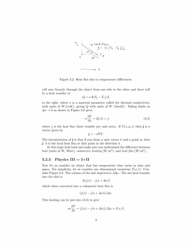
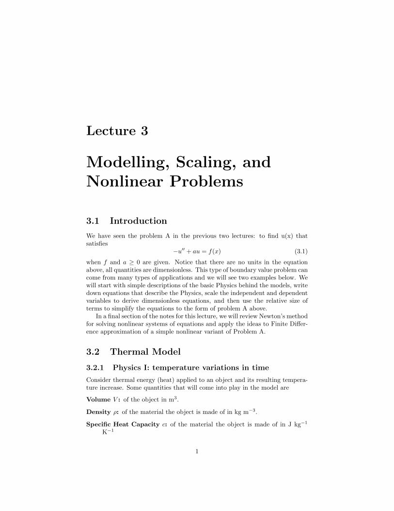
Figure 3.2: Heat flux due to temperature differences.

will vary linearly through the object from one side to the other and there willbe a heat transfer of

Q = κA(T0 − T1)/L

to the right, where κ is a material parameter called the thermal conductivity,with units of W/(mK), giving Q with units of W (check!). Taking limits as∆x→ 0 as shown in Figure 3.2 gives

−κ∂T∂x

= Q/A := j (3.4)

where j is the heat flux (heat transfer per unit area). If T (x, y, z) then j is avector given by

j = −κ∇T.

The interpretation of j is that if you chose a unit vector n̂ and a point x, thenj · n̂ is the local heat flux at that point in the direction n̂.

At this stage look back and make sure you understand the difference betweenheat (units of W, Watt), volumetric heating (W/m3), and heat flux (W/m2).

3.2.3 Physics III = I+II

Now let us consider an object that has temperature that varies in time andspace. For simplicity, let us consider one dimensional variations T (x, t). Con-sider Figure 3.3. The volume of the slab depicted is A∆x. The net heat transferinto the slab is

A(j(x)− j(x+ ∆x))

which when converted into a volumetric heat flux is

(j(x)− j(x+ ∆x))/∆x.

This heating can be put into (3.3) to give

ρc∂T

∂t= (j(x)− j(x+ ∆x))/∆x+ f(x, t)

3

Figure 3.3: Derivation of the one dimensional heat equation.

where f is a true volumetric heating term. Taking the limit as ∆x → 0 in theequation above and using (3.4) gives

ρc∂T

∂t= κTxx + f

known as the heat equation. Note that if κ(x) then if we look back through theargument we will find that

ρc∂T

∂t=

∂

∂x(κTx) + f

In three spatial dimensions, the same type of argument (using a little cubeinstead of a thin slab) gives

ρc∂T

∂t= κ∆T + f (3.5)

where here we have taken κ constant again and ∆ here is the Laplacian operator,∆T = Txx + Tyy + Tzz.

3.2.4 Heat transfer in a rod: scaling and reduced problem

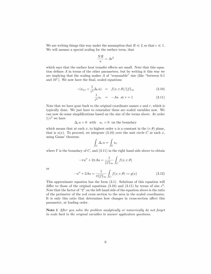
Consider heat transfer in the rod shown in Figure 3.4. It is described by theequation we derived above (3.5)

ρc∂T

∂t= κ(Txx + ∆rT ) + f(x, r, θ) (3.6)

where we have written the Laplacian in cylindrical coordinates,

∆rT =1

r2Tθθ +

1

r(rTr)r.

4

The rod is in an environment with ambient temperature TAMB. Heat is ex-changed to the environment at the boundary of the rod according to the rela-tionship

κTr |r=R = N(TAMB − T |r=R ) (3.7)

whereN is a given parameter determined experimentally, with units of W/(m2K).The relationship (3.7) is a crude approximation to the transfer of heat to theexternal environment, but can be justified in some situations. For this example,I will ignore what happens at the x = 0 and x = L boundaries.

Assume that the system reaches steady state with T independent of t andthen

−κ(Txx + ∆rT ) = f(x, r, θ). (3.8)

We will non-dimensionalize the equation (3.8) and boundary condition (3.7) ina series of steps. First, we shift the temperature to be relative to ambient:

v = T − TAMB

which still satisfies (3.8) but now the boundary condition (3.7) is homogeneousfor v:

κvr |r=R = −Nv |r=R (3.9)

Then we will scale x and r in the natural way by L and R respectively, givingnon-dimensional variables X and s both in [0,1] with

x = XL and r = sR

Putting these into (3.8) and (3.9) gives

−(vXX +L2

R2∆sv) =

L2

κf(x, r, θ)

vs = −NRκv at s = 1

For linear problems, scaling for the unknown is a bit arbitrary, but here it makessense to take the non-dimensional temperature u with v = τu with temperaturescale

τ =L2

κ‖f‖∞

(check that τ has units of K!). Now the scaled equations are

−(uXX +L2

R2∆su) = f(X, s, θ)/‖f‖∞

us = −NRκu at s = 1

and we see that there are two dimensionless parameters ε = R/L, the aspectratio of the rod, and NR

κ , the ratio of surface to internal heat transfer effects.

5

We are writing things this way under the assumption that R� L so that ε� 1.We will assume a special scaling for the surface term, that

NR

κ= Aε2

which says that the surface heat transfer effects are small. Note that this equa-tion defines A in terms of the other parameters, but by writing it this way weare implying that the scaling makes A of “reasonable” size (like “between 0.1and 10”). We now have the final, scaled equations

−(uxx +1

ε2∆ru) = f(x, r, θ)/‖f‖∞ (3.10)

1

ε2ur = −Au at r = 1 (3.11)

Note that we have gone back to the original coordinate names x and r, which istypically done. We just have to remember these are scaled variables now. Wecan now do some simplifications based on the size of the terms above. At order1/ε2 we have

∆ru = 0 with ur = 0 on the boundary

which means that at each x, to highest order u is a constant in the (r, θ) plane,that is u(x). To proceed, we integrate (3.10) over the unit circle C at each x,using Gauss’ theorem: ∫

C

∆ru =

∫Γ

ur

where Γ is the boundary of C, and (3.11) in the right hand side above to obtain

−πu′′ + 2πAu =1

‖f‖∞

∫C

f(x, r, θ)

or

−u′′ + 2Au =1

π‖f‖∞

∫C

f(x, r, θ) := g(x) (3.12)

This approximate equation has the form (3.1). Solutions of this equation willdiffer to those of the original equations (3.10) and (3.11) by terms of size ε2.Note that the factor of “2” on the left hand side of the equation above is the ratioof the perimeter of the rod cross section to the area in the scaled coordinates.It is only this ratio that determines how changes in cross-section affect thisparameter, at leading order.

Note 1 After you solve the problem analytically or numerically do not forgetto scale back to the original variables to answer application questions.

6

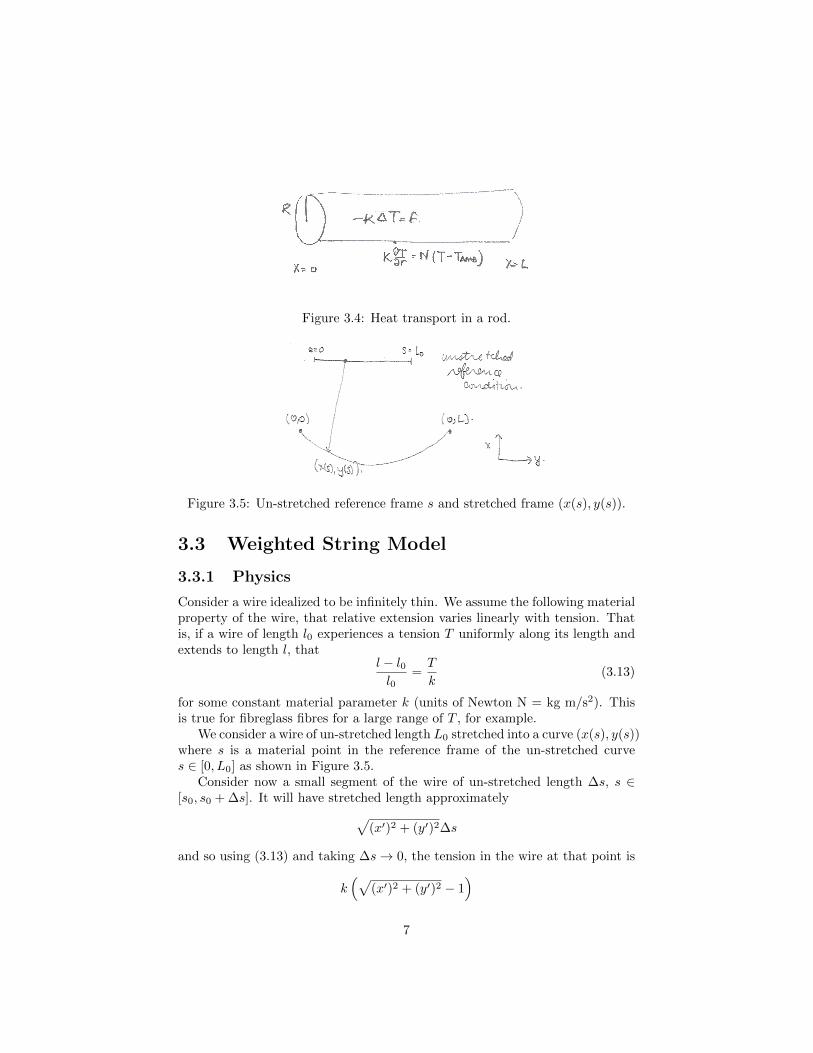
Figure 3.4: Heat transport in a rod.

Figure 3.5: Un-stretched reference frame s and stretched frame (x(s), y(s)).

3.3 Weighted String Model

3.3.1 Physics

Consider a wire idealized to be infinitely thin. We assume the following materialproperty of the wire, that relative extension varies linearly with tension. Thatis, if a wire of length l0 experiences a tension T uniformly along its length andextends to length l, that

l − l0l0

=T

k(3.13)

for some constant material parameter k (units of Newton N = kg m/s2). Thisis true for fibreglass fibres for a large range of T , for example.

We consider a wire of un-stretched length L0 stretched into a curve (x(s), y(s))where s is a material point in the reference frame of the un-stretched curves ∈ [0, L0] as shown in Figure 3.5.

Consider now a small segment of the wire of un-stretched length ∆s, s ∈[s0, s0 + ∆s]. It will have stretched length approximately√

(x′)2 + (y′)2∆s

and so using (3.13) and taking ∆s→ 0, the tension in the wire at that point is

k(√

(x′)2 + (y′)2 − 1)

7

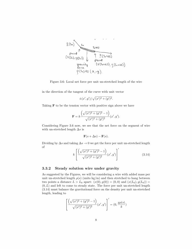
Figure 3.6: Local net force per unit un-stretched length of the wire

in the direction of the tangent of the curve with unit vector

±(x′, y′)/√

(x′)2 + (y′)2.

Taking F to be the tension vector with positive sign above we have

F = k

(√(x′)2 + (y′)2 − 1

)√

(x′)2 + (y′)2(x′, y′).

Considering Figure 3.6 now, we see that the net force on the segment of wirewith un-stretched length ∆s is

F(s+ ∆s)− F(s).

Dividing by ∆s and taking ∆s→ 0 we get the force per unit un-stretched lengthof

k

(√

(x′)2 + (y′)2 − 1)

√(x′)2 + (y′)2

(x′, y′)

′ (3.14)

3.3.2 Steady solution wire under gravity

As suggested by the Figures, we will be considering a wire with added mass perunit un-stretched length ρ(s) (units kg/m) and then stretched to hang betweentwo points a distance L > L0 apart: (x(0), y(0)) = (0, 0) and (x(L0), y(L0)) =(0, L) and left to come to steady state. The force per unit un-stretched length(3.14) must balance the gravitational force on the density per unit un-stretchedlength, leading to

(√(x′)2 + (y′)2 − 1

)√

(x′)2 + (y′)2(x′, y′)

′ = (0,gρ(s)

k)

8

We scale s by L0, x by L, y by Y to be determined later, and obtain the scaledequations

(√(x′)2 + (y′Y/L)2 − L0/L

)√

(x′)2 + (y′Y/L)2(x′, y′Y/L)

′ = (0,L2

0

L

gρ(s)

k)

It is now clear that the right scale for Y is

Y = L20

g‖ρ‖∞k

(units of m, check!) and to proceed we will assume now that

Y/L := ε� 1

leading to (√

(x′)2 + (εy′)2 − L0/L)

√(x′)2 + (εy′)2

(x′, y′)

′ = (0, ρ(s)/‖ρ‖∞)

At highest order (neglecting the terms of size ε) the equations decouple. The firstcomponent is satisfied if x′ is constant and to match the scaled end conditionswe have x ≡ s. For y we have

y′′ = ρ(s)/‖ρ‖∞1

1− L0/L

with y(0) = 0 and y(1) = 0 and we can think of the independent variable as xinstead of s.

3.4 Solving Nonlinear Systems with Newton’sMethod

3.4.1 Review of scalar Newton’s method

Consider solving for the root x∗ of a scalar equation:

f(x∗) = 0.

Begin with a relatively accurate estimate x0 of the root, and the linear (tangentline) approximation of f(x) based at x0 as shown in Figure 3.7. We take as thenext approximation x1, the root of the tangent line. That is, x1 satisfies

f(x0) + f ′(x0)(x1 − x0) = 0

which can be solved for

x1 = x0 −f(x0)

f ′(x0)

9

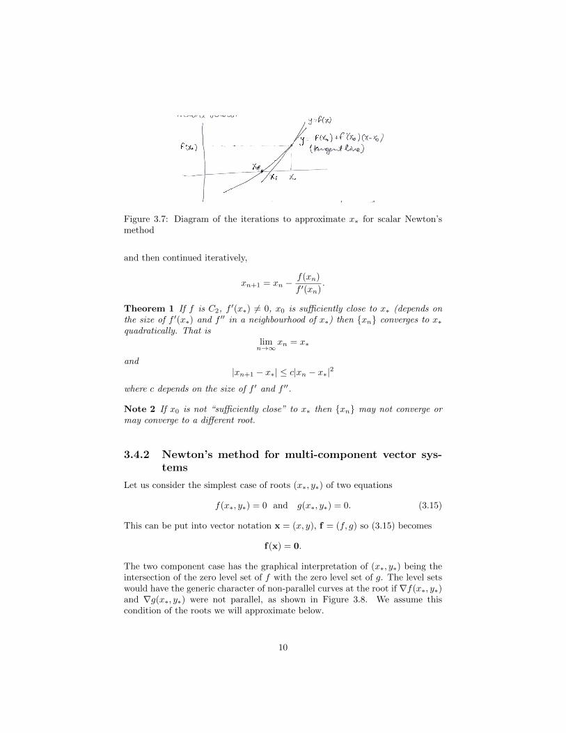
Figure 3.7: Diagram of the iterations to approximate x∗ for scalar Newton’smethod

and then continued iteratively,

xn+1 = xn −f(xn)

f ′(xn).

Theorem 1 If f is C2, f ′(x∗) 6= 0, x0 is sufficiently close to x∗ (depends onthe size of f ′(x∗) and f ′′ in a neighbourhood of x∗) then {xn} converges to x∗quadratically. That is

limn→∞

xn = x∗

and|xn+1 − x∗| ≤ c|xn − x∗|2

where c depends on the size of f ′ and f ′′.

Note 2 If x0 is not “sufficiently close” to x∗ then {xn} may not converge ormay converge to a different root.

3.4.2 Newton’s method for multi-component vector sys-tems

Let us consider the simplest case of roots (x∗, y∗) of two equations

f(x∗, y∗) = 0 and g(x∗, y∗) = 0. (3.15)

This can be put into vector notation x = (x, y), f = (f, g) so (3.15) becomes

f(x) = 0.

The two component case has the graphical interpretation of (x∗, y∗) being theintersection of the zero level set of f with the zero level set of g. The level setswould have the generic character of non-parallel curves at the root if ∇f(x∗, y∗)and ∇g(x∗, y∗) were not parallel, as shown in Figure 3.8. We assume thiscondition of the roots we will approximate below.

10

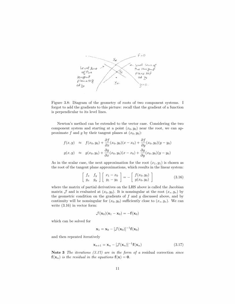
Figure 3.8: Diagram of the geometry of roots of two component systems. Iforgot to add the gradients to this picture: recall that the gradient of a functionis perpendicular to its level lines.

Newton’s method can be extended to the vector case. Considering the twocomponent system and starting at a point (x0, y0) near the root, we can ap-proximate f and g by their tangent planes at (x0, y0):

f(x, y) ≈ f(x0, y0) +∂f

∂x(x0, y0)(x− x0) +

∂f

∂y(x0, y0)(y − y0)

g(x, y) ≈ g(x0, y0) +∂g

∂x(x0, y0)(x− x0) +

∂g

∂y(x0, y0)(y − y0)

As in the scalar case, the next approximation for the root (x1, y1) is chosen asthe root of the tangent plane approximations, which results in the linear system:[

fx fygx gy

] [x1 − x0

y1 − y0

]= −

[f(x0, y0)g(x0, y0)

](3.16)

where the matrix of partial derivatives on the LHS above is called the Jacobianmatrix J and is evaluated at (x0, y0). It is nonsingular at the root (x∗, y∗) bythe geometric condition on the gradients of f and g discussed above, and bycontinuity will be nonsingular for (x0, y0) sufficiently close to (x∗, y∗). We canwrite (3.16) in vector form:

J (x0)(x1 − x0) = −f(x0)

which can be solved for

x1 = x0 − [J (x0)]−1f(x0)

and then repeated iteratively

xn+1 = xn − [J (xn)]−1f(xn) (3.17)

Note 3 The iterations (3.17) are in the form of a residual correction sincef(xn) is the residual in the equations f(x) = 0.

11

Remember that we never compute matrix inverses, so although (3.17) is anice form for the iterations, we actually compute

Jnun = −f(xn)

xn+1 = xn + un.

The methods extend to the N vector case f(x) = 0 with the Jacobian matrixN ×N with entries

Ji,j =∂fi∂xj

.

An important example of nonlinear systems comes in the optimization (max-imization of minimization) of functions of many variables f(x) (scalar f). Theoptimal value occurs at critical points that satisfy ∇f = 0, which is a nonlinearsystem of N equations in N unknowns. In this case, the Jacobian matrix of ∇fis the Hessian matrix of f ,

Ji,j =∂2f

∂xi∂xj.

Note that in this case J is symmetric, and near a generic local minimum it ispositive definite, so there are good solver options for the Newton updates.

3.4.3 Application to finite difference methods

We have seen in section 3.3 that physical models can be nonlinear. Let usconsider the simplest nonlinear model relative of problem A, with nonlinearityin u but not in derivatives. An example is given below, for u(x) 1-periodic in x:

−u′′ + u+ u3 = f(x). (3.18)

We could make a finite difference discretization as usual including the nonlin-earity:

−(Uj−1 − 2Uj + Uj+1)/h2 + Uj + U3j − Fj = 0

which is a nonlinear system. We can do Newton iterations U(m) to approximatethe solution to the system. The Jacobian matrix J at the m’th update hasentries

Ji,j =

−1/h2 if j = i− 1 or j = i+ 1

2/h2 + 1 + 3[U(m)j ]2 if j = i

0 otherwise

where the indices are taken modN . We see that J = A+diag{3[U(mj )]2} where

A is the matrix from the linear problem A. A MATLAB implementation for thisproblem will be provided.

Note 4 Iterates converge to the exact solution U of the discrete problem, butnot to the exact solution to the continuum problem (3.18). We will want theiteration error to be smaller that the discretization error so as not to confuse the

12

accuracy of the result. On the other hand, we should not spend too many com-putational resources on making this much more accurate than the discretizationerror. If you really understand the properties of the method, you would balancethe accuracy to computational cost benefit.

For some nonlinear problems, finding an initial vector U(0) close enough tothe exact solution so that Newton iterations converge can be very difficult. Thatis not true for the problem (3.18) for which it can be proved that the iterationsconverge for any initial guess (it is a convex problem). However, let us usethis as an example, and explain a technique that can solve the issue of havinga good initial vector. Consider (3.18) as a family of problems indexed by thescalar θ ∈ [0, 1]:

−D2Uj + Uj + θU3j = Fj .

There is a continuous family of solutions U(θ) and we want U(1). The solutionU(0) is easy to find, it is just the discretization of the original, linear problemA. If we had the solution U(θ) for θ ∈ (0, 1) it would be a good initial guessfor Newton’s method for U(θ + ∆θ) for ∆θ sufficiently small. Thus we couldmove from θ = 0 to θ = 1 with ∆θ adaptively reduced as needed to guaranteeconvergence of the Newton iterations at each step. This technique is calledcontinuation.

3.5 Problems

Problem 1 Consider the heat conduction problem in Section 3.2. If the surfaceheat transfer term has a different scaling, that is

NR

κ= O(1)

derive the leading order behaviour in this case.

Problem 2 Identify the problem for the next order correction in the heat con-duction problem in Section 3.2. That is, consider the scaled equations (3.10,3.11). Assume that the solution has the asymptotic expansion

u(x, r, θ) = u(x) + ε2v(x, r, θ) +O(ε4)

where u(x) is the solution to the problem (3.12) we identified as describing thedominant effects. Find the equations for v. Often, u above is denoted by u(0)

and v by u(2) to denote the orders that they appear in the expansion.

Problem 3 Identify the next order correction in the weighted string model equa-tions.

Problem 4 Consider the nonlinear boundary value problem (3.18). Show exis-tence and uniqueness of solutions and the regularity of solutions in terms of the

13

data f . If you want a harder equation to prove things about, try the the nonlin-ear weighted string model equations. Note that negative tension is not physical(leads to ill-posedness), so show that this does not occur in the solutions to themodel.

Problem 5 Write a Finite Difference discretization of the nonlinear stringproblem. Find solutions using Newton’s method. Show numerically that as ε→ 0the solutions tend those of the linear problem.

14