Survey of Gain-Scheduling Analysis & Design

D.J.LeithWE.Leithead

Department of Electronic & Electrical Engineering,University of Strathclyde, 50 George St., Glasgow G1 1QE

Tel. 0141 548 2407 Fax. 0141 548 4203 Email. doug@icu.strath.ac.uk

AbstractThe gain-scheduling approach is perhaps one of the most popular nonlinear control design approaches which hasbeen widely and successfully applied in fields ranging from aerospace to process control. Despite the wideapplication of gain-scheduling controllers and a diverse academic literature relating to gain-scheduling extendingback nearly thirty years, there is a notable lack of a formal review of the literature. Moreover, whilst much ofthe classical gain-scheduling theory originates from the 1960s, there has recently been a considerable increase ininterest in gain-scheduling in the literature with many new results obtained. An extended review of the gain-scheduling literature therefore seems both timely and appropriate. The scope of this paper includes the maintheoretical results and design procedures relating to continuous gain-scheduling (in the sense of decompositionof nonlinear design into linear sub-problems) control with the aim of providing both a critical overview and auseful entry point into the relevant literature.

1. IntroductionGain-scheduling is perhaps one of the most popular approaches to nonlinear control design and has been

widely and successfully applied in fields ranging from aerospace to process control. Although a wide variety ofcontrol methods are often described as “gain-scheduling” approaches, these are usually linked by a divide andconquer type of design procedure whereby the nonlinear control design task is decomposed into a number oflinear sub-problems. This divide and conquer approach is the source of much of the popularity of gain-scheduling methods since it enables well established linear design methods to be applied to nonlinear problems.(Whilst the analysis and design of nonlinear systems remains relatively difficult, techniques for the analysis anddesign of linear time-invariant systems are rather better developed). However, it is also emphasised that thebenefits of continuity with linear methods often extend beyond purely technical considerations; for example,safety certification requirements are often based on linear methods and the development of new certificationprocedures using nonlinear approaches may well be prohibitive. Of course, the question must be asked as towhether the basic premise of such design approaches is in fact reasonable; that is, whether a wide class ofnonlinear design tasks can genuinely be decomposed into linear sub-problems. While few results are availablewhich relate directly to this fundamental issue, and it is well known that certain classes of problem presentgreater difficulty than others for gain-scheduling methods, the general usefulness of such methods is neverthelesswell established both in practice and from a theoretical viewpoint.

Despite the wide application of gain-scheduling controllers and a diverse academic literature relating to gain-scheduling extending back nearly thirty years, there is a notable lack of a formal review of the literature.Moreover, whilst much of the classical gain-scheduling theory originates from the 1960s, there has recently beena considerable increase in interest in gain-scheduling in the literature with many new results obtained. A reviewof the gain-scheduling literature therefore seems both timely and appropriate. It is, unfortunately, impossible tocover the great wealth of gain-scheduling literature within the available space and the scope of this paper is thusnecessarily limited. Firstly, no attempt is made to review the vast literature detailing specific applications ofgain-scheduling methods. Secondly, in order to retain a reasonable focus to the paper, consideration is confinedto methods based on the decomposition of the nonlinear design task into linear sub-problems; accordingly, themany interesting approaches based on decomposing the design task into simpler nonlinear sub-problems(including those involving decomposition into affine sub-problems) are not discussed. Thirdly, attention isrestricted to continuous scheduling methods and no attempt is made to review the very extensive literature onhybrid/switched systems. The scope of the paper is thus restricted to the main theoretical results and designprocedures relating to continuous gain-scheduling (in the sense of decomposition of nonlinear design into linearsub-problems) control and the aim is to provide a critical overview and useful entry point into the relevantliterature. The subject matter covered clearly remains considerable and it has sometimes been difficult toachieve a satisfactory balance between the requirement to provide a concise critical overview of the field whilecovering the subject in reasonable detail. In addition, although substantial effort has been expended in strivingto present as balanced perspective as possible on alternative methodologies, the reader should be aware thatsome degree of subjective judgement is surely inevitable. Any such deficiencies do not, of course, necessarilyreflect the opinions of others.

The paper is organised as follows. The theoretical results relating the dynamic characteristics of a nonlinearsystem to those of a family of linear systems are reviewed in section 2. The classical gain-scheduling designprocedure is discussed in section 3 followed by a number of recent divide and conquer approaches which attemptto address a number of deficiencies of classical methods. LPV gain-scheduling approaches, which have recentlybeen the subject of considerable research activity but are less strongly based on divide and conquer ideas, arereviewed in section 4 and the outlook is briefly discussed in section 5. The notation used is standard (seeAppendix A).

2. L inear isation theoryGain-scheduling design typically employs a divide and conquer approach whereby the nonlinear design task

is decomposed into a number of linear sub-tasks. Such a decomposition depends on establishing a relationshipbetween a nonlinear system and a family of linear systems. The main theoretical results which, for a broad classof nonlinear systems, relate the dynamic characteristics of a member of the class to those of an associated familyof linear systems are reviewed in this section. These results fall into two main sub-classes. First, stability resultswhich establish a relationship between the stability of a nonlinear system and the stability of an associated linearsystem. Second, approximation results which establish a direct relationship between the solution to a nonlinearsystem and the solution to associated linear systems. It is important to distinguish between these classes ofresult. The former are typically much more limited than the latter, being confined to specifying conditionsunder which boundedness of the solution to a particular linear system implies boundedness of the solution to thenonlinear system for an appropriate class of inputs and initial conditions. Notice that under such conditions thesolutions are bounded but may otherwise be quite dissimilar. Reflecting this distinction, the discussion in thefollowing sections often separately considers results relating both to stability and approximation.

The section is organised as follows. Perhaps the most widespread approach for associating a linear systemwith a nonlinear one, namely series expansion linearisation theory, is first reviewed The literature relating toseries expansion linearisations is, of course, extensive yet, unfortunately, also very fragmented and it isnecessary to consolidate many separate results in writing this review. The approach taken here is, therefore, toprovide an overview of the available body of theory in section 2.1 while referring the reader to Appendix B fordetailed references. The series expansion linearisation is only valid in the vicinity of a specific trajectory orequilibrium point, and so there is considerable incentive to develop techniques which relax this restriction.Approaches which aim to increase the allowable operating envelope by utilising a family of linearisations (ratherthan just a single linearisation) are reviewed in sections 2.2-2.3.

2.1Ser ies expansion linearisation about a single trajectory or equilibr ium point1

The series expansion linearisation of a nonlinear system is well known. Consider the nonlinear system,�x = F(x, r ), y = G(x, r ) (1)

where r ∈ ℜm, y ∈ ℜp, x ∈ ℜn. Let ( ~x (t), ~r (t), ~y (t)) denote a specific trajectory of the nonlinear system (the

trajectory could simply be an equilibrium operating point in which case ~x is constant). Neglecting higher-orderterms, it follows from series expansion theory that the nonlinear system, (1), may be approximated, locally to thetrajectory, ( ~x (t), ~r (t), ~y (t)), by the linear time-varying system

δ� �x = ∇xF( ~x , ~r )δ

�x + ∇rF( ~x , ~r )δr (2)

δ�y = ∇xG( ~x , ~r )δ

�x + ∇rG( ~x , ~r )δr (3)

whereδr = r - ~r , y = δy + ~y , δx = x - ~x (4)

Clearly, the nonlinear system, (1), is stable relative to the trajectory ( ~x (t), ~r (t), ~y (t)) provided the linear time-varying dynamics (2)-(3) are robustly stable with respect to the approximation error involved in truncating theseries expansion. In fact, is turns out that nonlinear system, (1), is locally BIBO stable if and only if the linearsystem (2)-(3) is exponentially stable when δr is zero (i.e. the unforced case) (see, for example, Khalil 1992p184, Vidyasagar & Vannelli 1982).

In the special case when the system, (2)-(3), is linear time-invariant, simple necessary and sufficientconditions for its stability are well-known (see, for example, Vidyasagar 1993). However, in the time-varyingcase, the stability analysis is, in general, not so straightforward. In the context of gain-scheduling, frozen-timetheory is widely employed to establish stability conditions for linear time-varying systems. Specifically, it canbe shown(see, for example, Desoer 1969, Ilchmann et al. 1987) that the stability of the linear time-varyingsystem, (2)-(3), is guaranteed provided that the time variation of ∇xF( ~x , ~r ) is sufficiently slow in someappropriate sense (for example, that ( ) |)~,~F(d/dt| sup

0trxx∇

≥ is sufficiently small). Although classical frozen-time

results mainly relate to nominal stability, it can also be shown that, provided the rate of variation is sufficiently 1 See also Appendix B

slow, the linear time-varying system (2)-(3) inherits the worst-case stability robustness of the family of frozen-

time linear time-invariant systems δ� �x = Aτδ

�x where Aτ denotes the value of ∇xF( ~x , ~r ) at time τ (Barman

1973, Shamma & Athans 1991, Leith & Leithead 1998b). Frozen-time theory is generally conservative in that itonly establishes sufficient conditions for stability. In addition, it is important to note that in all of the frozen-time robustness results an increase in robustness requires a decrease in the allowable rate of variation and thatthe linear time-varying system fully inherits the robustness of the frozen-time family only as the allowable rateof variation becomes arbitrarily small.

The foregoing results relate to stability properties only. Were the linear dynamics, (2)-(3), an accurateapproximation to the nonlinear dynamics, (1), then it might be expected that, when starting from the same initialconditions, the solutions of (1) and (2)-(3) remain correlated for some time. However, the solution to (2)-(3) is,in fact, only a zeroeth order approximation to the solution to (1) (see, for example, Leith & Leithead 1998b).This poor approximation property is inevitably reflected in the weakness of any approximation result; forexample, Desoer & Wong (1968) and Desoer & Vidyasagar (1975 section 4.9). These results state that the peakabsolute difference between the solution, δ

x , of the approximate system, (2)-(3), and the solution, δx, of the

nonlinear system, (1), is bounded provided the approximate system, (2)-(3), is stable, δr is sufficiently small andthe initial conditions, δx(0) and δ

x (0), are zero (although it is straightforward to extend this to encompass non-

zero initial conditions which are sufficiently close to the origin). It can be seen that this result is, essentially, arestatement of local BIBO stability; that is, simply that the solutions of (1) and (2)-(3) both remain within abounded region enclosing the origin provided the input and the initial conditions are sufficiently small.

2.2Ser ies expansion linearisation familiesThe foregoing results are confined to the dynamic behaviour locally to a single trajectory or equilibrium

operating point. This is a significant limitation of the series expansion linearisation theory particularly since thelocal neighbourhood within which the analysis is valid may, in general, be very small. Within a gain-schedulingcontext, it is almost always required to consider the behaviour of a system relative to a family of operatingpoints, which spans the envelope of operation, rather than relative to a single operating point. In order toincrease the size of the operating region within which a series expansion linearisation is valid, it is thereforenatural to consider combining, in some sense, the series expansion linearisations associated with a number ofequilibrium points. At this point it is perhaps worth emphasising the clear distinction which exists between asingle dynamic system and a family of dynamic systems, regardless of any superficial similarity between thetwo. The linear time-varying system (2)-(3),for example, is a quite different object (being a distinct dynamicsystem) from the associated family of frozen linear time-invariant systems (being a collection of dynamicsystems). The importance of this distinction becomes particularly great when the state, input and/or output of themembers of the family differ from one another as is the case when considering the family of series expansionlinearisations of (1) relative to the equilibrium points. The state, input and output of each series expansionlinearisation are perturbation quantities which depend on the equilibrium point considered. The relationshipbetween the solution to a nonlinear system and the solutions to its series expansion linearisations is thus notstraightforward when the system is not confined to the vicinity of a single equilibrium point. Nevertheless, it ispossible to establish a weaker relationship. Namely, a relationship between the local stability of a nonlinearsystem and the stability of the associated series expansion equilibrium linearisations.

The relevant theory stems primarily from an early lemma by Hoppensteadt (1966) (see also Khalil &Kokotovic 1991, Khalil 1992 chapter 4, Lawrence & Rugh 1990) originally derived in the context of singularperturbation theory. Using this so-called frozen-input theory, it can be shown that the nonlinear system, (1), islocally BIBO stable in the vicinity of equilibrium operation provided that the members of its family ofequilibrium linearisations are uniformly stable and the rate of variation is sufficiently slow. In addition, a trivialextension of this result is that, provided that the rate of variation is sufficiently slow, the nonlinear system alsoinherits the stability robustness of the equilibrium linearisations to smooth, finite dimensional, nonlinearperturbations (although there is the usual trade-off between robustness and the restrictiveness of the slowvariation condition required). The slow variation condition in these results generally takes the form of arestriction both on the initial conditions of the system and on the rate of variation of the forcing input. This slowvariation condition plays two roles: firstly, it ensures that the system stays sufficiently near to equilibriumoperation (necessary owing to the use of equilibrium linearisations) and secondly, it ensures that the systemevolves sufficiently slowly from the vicinity of one equilibrium point to the vicinity of another. It is emphasisedthat the analysis is inherently confined to a small neighbourhood enclosing the equilibrium operating points andconsequently may be extremely conservative. Such a restriction is, of course, to be expected since the analysis isbased on the properties of the series expansion linearisations of the nonlinear plant relative to the equilibriumpoints and so only utilises information regarding the dynamics at equilibrium. It is also worth noting that it isoften difficult to test whether the stability conditions obtained are satisfied since they typically involve quantitieswhich are difficult to evaluate (Shamma & Athans 1990). Indeed, perhaps owing to this difficulty, although

frozen-input results are widely invoked in the literature to justify control designs it is quite rare for thetheoretical slow variation conditions applying in a particular application to be actually determined.

An additional technical requirement in frozen-input stability analysis is that the equilibrium operating pointsare smoothly parameterised by the system input, r . This requirement is not unduly restrictive in an analysiscontext but may be undesirable in the gain-scheduling design context, where it is more natural to parameterisethe equilibrium operating points by the scheduling variable. It is perhaps interesting to note that Shamma &Athans (1990 section 4) apparently attempt to extend this type of analysis to a class of systems with a particularfeedback structure and for which the family of equilibrium operating points is parameterised by a subset of thesystem states, y, rather than the input, r (see Appendix C). The “output” y and the system dynamics mutuallyinteract with one another whereas the input, r , is independent of the system dynamics. Consequently, theanalysis of an “output” scheduled nonlinear system is more difficult than the input-scheduled case. Shamma &Athans (1990) establish stability conditions requiring that |

�y | is sufficiently small and, in addition, that the

magnitude of the input, r , and initial condition of a certain transformed state vector, ξ, are sufficiently small.The latter conditions confine the analysis, in general, to trajectories, (ξ(t), r (t)) which lie within a small regionenclosing the origin (see, for example, Shamma & Athans 1990, theorem 4.4). Since y, which parameterises theequilibrium operating point, is a subset of the transformed states, ξ, (see Appendix C) it follows that y(t) is alsoconfined to a region enclosing the origin. Hence, the analysis cannot in general be applied to an extended familyof equilibrium operating points as generally required in a gain-scheduling context.

2.3Off-equilibr ium linear isationsConventional series expansion theory associates a linear time-invariant system only with equilibrium

operating points. Consequently, any analysis/design based on this theory is generally only valid during nearequilibrium operation. This limitation arises due to the characteristics of conventional series expansions but maybe resolved by, instead, considering an alternative linearisation framework.

Before proceeding, in order to streamline the later discussion it is useful to explicitly highlight the linear andnonlinear dependencies of the dynamics by reformulating the nonlinear system (1) as�

x = Ax + Br + f(ρ), y = Cx + Dr + g(ρ) (5)where A, B, C, D are appropriately dimensioned constant matrices, f(•) and g(•) are nonlinear functions andρ(x,r ) embodies the nonlinear dependence of the dynamics on the state and input with ∇xρ, ∇rρ constant.Trivially, this reformulation can always be achieved by letting ρ = [xT r T]T. However, the nonlinearity of thesystem is frequently dependent on only a subset of the states and inputs, in which case the dimension of ρ isreduced. The formulation, (5), defines a scheduling variable ρ which explicitly embodies the nonlineardependence of the dynamics.

It may be shown (Leith & Leithead 1998b) that the solution to the velocity-based linearisation �x =

�w (6)� �

w = (A+∇f(ρ1))�w + (B+∇f(ρ1))

�r (7)� �

y = (C+∇g(ρ1))�w + (D+∇g(ρ1))

�r (8)

approximates the solution to the nonlinear system, (5) (and so (1)), locally to an operating point (x1, r 1) at whichρ1=ρ(x1, r 1). It is emphasised that (x1, r 1) may be a general operating point (it need not be an equilibrium pointand, indeed, may lie far from any equilibria). While the solution to the velocity-based linearisation is only alocal approximation, there is a velocity-based linearisation associated with every operating point of a nonlinearsystem and the solutions to these linearisations may be pieced together to globally approximate the solution tothe nonlinear system, (5), to an arbitrary degree of accuracy. Hence, the velocity-based linearisation familyembodies the entire dynamics of a nonlinear system, with no loss of information, and is, in fact, an alternativerepresentation of the nonlinear system. The velocity-based linearisation family is parameterised by thescheduling variable, ρ, and in this sense ρ captures the nonlinear structure of a system. The relationship betweenthe nonlinear system, (5), and its velocity-based linearisation, (6)-(8), is direct. Differentiating (5), an alternativerepresentation of the nonlinear system is�

x = w (9)�w = (A+∇f(ρ))w + (B+∇f(ρ))

�r (10)�

y = (C+∇g(ρ))w + (D+∇g(ρ))�r (11)

Evidently, the velocity-based linearisation, (6)-(8), is simply the frozen form of (9)-(11) at the operating point,(x1, r1).

The relationship between the solution to a nonlinear system and the solutions to the members of theassociated velocity-based linearisation family can be used to derive conditions relating the stability of anonlinear system to the stability of its velocity-based linearisations. General stability analysis methods such assmall gain theory and Lyapunov theory can be applied to derive velocity-based stability conditions (including themethods in section 4). In addition, by adopting the velocity-based framework, it is possible to extend and

strengthen the classical frozen-input stability results discussed in section 2.2. Specifically, BIBO stability of thenonlinear system (1) is guaranteed provided the members of its velocity-based linearisation family are uniformlystable, unboundedness of the state x implies that w is unbounded (assuming the input r is bounded) and the classof inputs and initial conditions is restricted to limit the rate of evolution of the nonlinear system to be sufficientlyslow (Leith & Leithead 1998b). In addition, provided that the rate of evolution is sufficiently slow, the nonlinearsystem inherits the stability robustness of the members of the velocity-based linearisation family (Leith &Leithead 1998b) (with the usual trade-off between robustness and the restrictiveness of the slow variationcondition required).. This velocity-based result involves no restriction to near equilibrium operation other thanthat implicit in the slow variation requirement; for example, for some systems where the slow variation conditionis automatically satisfied the class of allowable inputs and initial conditions is unrestricted and the stabilityanalysis is global.

3. Divide & Conquer Gain-Scheduling DesignGain-scheduling design approaches conventionally construct a nonlinear controller, with certain required

dynamic properties, by combining, in some sense, the members of an appropriate family of linear time-invariantcontrollers. Design approaches may be broadly classified according to the linear family utilised. Classical gain-scheduling design approaches, based on the series expansion linearisation of a system about its equilibriumpoints, are discussed in section 3.1. Recent, and closely related, approaches based on neural/fuzzy modellingand off-equilibrium linearisations are considered, respectively, in sections 3.2 and 3.3.

3.1Classical gain-scheduling designConsider the nonlinear plant with dynamics, (1). The classical gain-scheduling design approach is based on

the family of equilibrium linearisations of the plant and may be applied directly to a broad range of nonlinearsystems. The design procedure typically involves the following steps (see, for example, Astrom & Wittenmark1989 section 9.5, Shamma & Athans 1990, Hyde & Glover 1993).

1. The equilibrium operating points of the plant are parameterised by an appropriate quantity, ρ, which mayinvolve the plant input, output and/or state.

2. The plant dynamics, (1), are approximated, locally to a specific equilibrium operating point, (xo,r o,yo), atwhich ρ equals ρo, by the series expansion linearisation,

δ� �x = ∇xF(xo(ρo), ro(ρo))δ

�x + ∇rF(xo(ρo), r o(ρo))δr (12)

δ y = ∇xG(xo(ρo), r o(ρo))δ

!x + ∇rG(xo(ρo), ro(ρo))δr (13)

δr = r - r o(ρo), "y = δ

#y + yo(ρo), δ

$x =

%x - xo(ρo) (14)

3. For a suitable controller input, e, with equilibrium value, eo(ρo), a linear time-invariant controller is designed,δ

&z= A(ρo)δz + B(ρo)δe (15)

δr = C(ρo)δz + D(ρo)δe (16)δe = e - eo(ρo), r = δr + r o(ρo) (17)

which ensures appropriate closed-loop performance when employed with the plant linearisation, (12)-(14). Itshould be noted that ρo is assumed to be constant when designing this linear controller. (While the controlleroutput equation, (16), is formulated assuming that every input to the plant is a controller output, it is, ofcourse, straightforward to accommodate situations where the controller output is only a subset of the inputs;for example, when the plant is subject to external disturbances).

4. Repeat steps 2 and 3 as required for a family of equilibrium operating points. A family of linear time-invariant controllers is obtained corresponding to the family of equilibrium operating points; both thecontroller family and the equilibrium operating points are parameterised by ρ. When a smoothly gain-scheduled controller is required, the linear controller designs are selected to have compatible structures whichpermit smooth interpolation between the designs.

With regard to the theoretical basis for smooth interpolation (as opposed to non-smooth), Kamen et al.(1989) note that when the plant linearisations are stabilizable at every equilibrium point, there exists astabilising family of static state feedback controllers the gains of which are continuously differentiablefunctions of the plant matrices,∇xF(xo(ρo), ro(ρo)),∇rF(xo(ρo), r o(ρo)),∇xG(xo(ρo), r o(ρo)), ∇rG(xo(ρo), r o(ρo)).More generally, when the plant linearisations are controllable at every equilibrium point, the poles of themembers of the closed-loop family can always be assigned by utilising a continuous family of dynamic statefeedback controllers (Sontag 1985).

With regard to constructive interpolation procedures, Stilwell & Rugh (1998) propose an interpolationapproach for state feedback and state feedback/observer based controllers which explicitly ensures stabilityof the closed-loop system at the interpolated operating points (at the cost of some conservativeness).However, relatively ad hoc interpolation schemes appear to be more commonly employed in practice. Inparticular, while more general approaches are certainly possible (see, for example, the fuzzy interpolationschemes proposed by Zhao et al. 1993, Qin & Borders 1994), it is usual to simply linearly interpolate eitherthe elements of the matrices in the state-space representation of the controller (e.g. Hyde & Glover 1993) orthe gain, poles and zeroes of the controller transfer functions (e.g. Nichols et al. 1993). The number ofmembers in the linear controller family employed is increased until satisfactory characteristics are obtained atthe interpolated points. It should be noted that there seem to be few theoretical results relating to the use oflinear interpolation. (With the notable exception of Shahruz & Behtash (1992) in the specific context of full-state feedback pole-placement control for a class of linear time-varying systems (namely LPV systems, seesection 6)).

5. Implement a nonlinear controller based on the family of linear controllers, (15)-(17). This step is ofconsiderable importance since the choice of nonlinear controller realisation can greatly influence the closed-loop performance (Leith & Leithead (1996), for example, observe in the context of wind turbine regulationthat the performance improvement obtained by employing a nonlinear gain-scheduled controller can beentirely lost by adopting a poor choice of nonlinear controller realisation). There are three main approachesto realising a nonlinear gain-scheduled controller2.

a. Classical approachFirstly, implement the controller input and output transformations, (17). It should be noted that this step is

often implicit. Typically, the controller input, e=y-yref, is zero (or near zero) in equilibrium (that is, eo(ρo)=0and δe = e) and either the plant exhibits pure integral action, so that r o(ρ) is identically zero, or each linearcontroller contains integral action which implicitly generates r o(ρ) through the action of the feedback loop(see, for example, Astrom & Wittenmark 1989 section 9.5, Shamma & Athans 1990, Hyde & Glover 1993).Alternatively, the controller output transformation may be implemented by explicitly calculating theequilibrium controller output as a function of ρ (see, for example, Rugh 1991, Shamma & Athans 1990).However, the latter approach may involve rather complex calculations which are sensitive to modellingerrors and, consequently, seems to be largely of theoretical interest (Hyde & Glover 1991).

Secondly, substitute ρ (or some related quantity) for ρo in the family of local linear controllers, (15)-(17),to obtain a nonlinear controller. It is noted that the scheduling variable need not be continuous; for example,it may be piece-wise constant, corresponding to switching between the members of the family of local linearcontrollers. Typically, the selection of an appropriate scheduling variable is based on physical insight(Astrom & Wittenmark 1989).

b. Local linear equivalenceA nonlinear controller realisation is selected for which the series expansion linearisation at each

equilibrium operating point matches the relevant member, (15)-(17), of the linear controller family (and ofcourse such that the family of controller equilibrium inputs and outputs agree with eo(ρ) and r o(ρ)). It shouldbe noted that nonlinear controller realisations obtained by traditional approaches (see preceding paragraph)need not satisfy this local linear equivalence condition. Wang & Rugh (1987a,b) give necessary andsufficient existence conditions for a linear controller family to be a linearisation family; that is, to correspondto the equilibrium linearisations of some nonlinear controller. These are extended to infinite dimensionalsystems by Banach & Baumann (1990). On the face of it, the existence conditions appear to be ratherrestrictive. However, it is very common for controllers to contain integral action to ensure rejection of steadydisturbances and in this case the existence conditions are readily satisfied (Kaminer et al. 1995, Lawrence &Rugh 1995). Specific classes of controller without integral action are also considered by Rugh (1991),Lawrence & Rugh (1995) but the proposed nonlinear controller realisations require a priori knowledge of theequilibrium controller output as a function of ρ in order to explicitly implement the input and outputtransformations, (17). Hence, they may involve rather complex calculations which are sensitive to modellingerrors (Hyde & Glover 1991).

2 The classical gain-scheduling approach is based on the plant linearisations at a number of equilibrium pointsand so utilises only information regarding the plant dynamics at equilibrium. The discussion in this section istherefore confined to controller realisation approaches based only on knowledge of the plant dynamics nearequilibrium. Methods which exploit additional information, particularly regarding the plant dynamics at non-equilibrium operating points, may lead to controller realisations which achieve better performance but areoutwith the scope of the conventional gain-scheduling approach; see later sections.

Given that the classical gain-scheduling approach only employs information about the plant dynamicslocally to the equilibrium points, the local linear equivalence condition seems to be quite reasonable and animprovement over traditional nonlinear controller realisation approaches. However, the local linearequivalence condition only requires that the nonlinear controller realisation has the required equilibriumlinearisations. The neighbourhoods within which the linearisations are an accurate description of thecontroller dynamics is not addressed. There exists an infinite number of nonlinear controller realisationssatisfying the local linear equivalence condition and the neighbourhoods within which the linearisations arevalid may be relatively large for some realisations but vanishingly small for others. The local linearequivalence condition does not distinguish between these realisations. As discussed in section 2.2.2, sincethe controller is designed on the basis only of the plant dynamics locally to the equilibrium points, arestriction to near equilibrium operation is inherent to the classical gain-scheduling approach. However, afurther restriction may be required to ensure that the system remains sufficiently near to equilibrium that thedynamics of the nonlinear controller are similar to those of the controller equilibrium linearisations; that is, tothe linear controller family designed at step 4. This latter restriction could be much stronger than thatassociated with the plant. The local linear equivalence condition entirely ignores this restriction: it may bevery strong for some controller realisations satisfying the local linear equivalence condition but relativelyweak for others. The local linear equivalence condition provides no guidance for distinguishing betweenthese realisations and this greatly diminishes its utility (Leith & Leithead 1998d, 1999c).

c. Extended local linear equivalenceIn order to address the deficiencies in the local linear equivalence approach, Leith & Leithead (1996,

1998a) propose that the nonlinear controller realisation should be selected to satisfy an extended local linearequivalence condition. The extended local linear equivalence condition selects, from the class of nonlinearcontroller realisations satisfying the local linear equivalence condition, those controller realisations whichmaximise, in an appropriate sense, the neighbourhoods within which the controller equilibrium linearisationsare an accurate description of the controller dynamics. Specifically, controller realisations are selected forwhich the individual neighbourhoods are unbounded and their union covers the entire operating space, Φ.Unnecessary restrictions on the operating envelope of the closed-loop system are thereby relaxed (in markedcontrast to realisations satisfying the local linear equivalence condition only). Whilst the extended locallinear equivalence condition is a strong requirement, controller realisations satisfying this condition for avery wide class of MIMO linear controller families are derived in Leith & Leithead (1998a). Similarly to thelocal linear equivalence condition, integral action has an important role in facilitating the realisation ofnonlinear controllers satisfying the extended local linear equivalence condition.

The classical gain-scheduling approach only employs information about the plant dynamics locally to theequilibrium points. In these circumstances, the extended local linear equivalence condition provides usefulguidance to selecting an appropriate nonlinear controller realisation and seems in some sense to be the “best”that can be achieved within the limitations imposed by knowing only equilibrium information (Leith &Leithead 1998a). However, this certainly does not mean that other choices of controller realisation may notbe superior, only that the analytic selection of such realisations seems to require further information about theplant dynamics. Methods for using additional information, particularly regarding the plant dynamics at non-equilibrium operating points, are outwith the scope of the classical gain-scheduling approach and arediscussed in later sections.

The foregoing gain-scheduling design process is frequently iterative, with the controller revised in the light ofsubsequent analysis until a satisfactory design is achieved.

The effectiveness of the classical gain-scheduling design approach depends on the dynamic characteristics ofthe nonlinear system, composed of the nonlinear plant and the nonlinear gain-scheduled controller, being relatedto those of the members of an associated family of linear systems, composed of the plant linearisations andcorresponding local linear controllers. Traditionally, the results reviewed in sections 2.1-2.2 are applied to relatethe dynamic characteristics of a nonlinear system to those of such an associated family of linear systems. Ofcourse, both series expansion linearisation theory (section 2.1.1) and frozen-input theory (section 2.2.2) areinherently restricted to operation near equilibrium. With regard to the support provided for the gain-schedulingdesign procedure, it is noted that these results consider only the stability properties of the nonlinear system andprovide little direct insight into other dynamic properties, such as the transient response. In addition, althoughfrozen-input theory can support the stability analysis of a nonlinear gain-scheduled control system about a familyof equilibrium points, it provides little insight into the controller design procedure since the frozen-inputrepresentation of the controlled system is quite distinct from the mixed series-expansion/frozen-schedulingvariable representation employed in step 3 of the design procedure. Series expansion linearisations of the plantare employed but the corresponding local controller designs are frozen-scheduling variable linearisations of theresulting nonlinear controller. In contrast, when analysing the dynamic behaviour of the controller locally to a

single equilibrium operating point using series expansion linearisation theory, the series expansion linearisationis employed instead of the frozen-scheduling variable linearisation. The frozen-input analysis of the controlledsystem in the vicinity of the family of equilibrium operating points does not reduce to either the series expansionanalysis (see, for example Shamma 1988 p110) or the mixed series-expansion/frozen-scheduling variableanalysis employed in the design procedure. The analysis of gain-scheduling design by means of conventionalresults, relating the dynamic characteristics of a nonlinear system to those of an associated family of linearsystems, is, therefore, rather convoluted and inefficient. The use of a variety of different local approximationsobscures insight and is unnecessary.

Remark Control of linear time-varying systemsGain-scheduled controllers are designed classically on the basis of the plant linearisations at a number of

equilibrium operating points. Of course, it follows from series expansion linearisation theory that a nonlinearsystem can be approximated by a linear system in the vicinity of a trajectory as well as in the vicinity of anequilibrium point. The linearisation relative to a trajectory is a linear time-varying, rather than linear time-invariant, system. Although rather less well developed than the control design methods for linear time-invariantsystems, control design methods for linear time-varying systems are considered in, for example, Ravi et al.(1991), Voulgaris & Dahleh (1995), Scherpen & Verhaegen (1996) (see also the methods discussed in section 4below). Whilst these approaches typically take a linear time-varying plant as the starting point for controldesign, Sontag (1987a,b) specifically considers control design for the family of linear time-varying systemscorresponding to the series expansion linearisations of a nonlinear plant relative to a family of trajectories forcontrol design. However, a fundamental limitation of any such approach for nonlinear systems is that thecontroller obtained is only valid in some small neighbourhood about a specific reference trajectory. In theclassical gain-scheduling approach, an attempt is made to enlarge the allowable operating region by combiningthe linear controllers associated with a number of the plant equilibrium linearisations. However, there do notappear to be comparable results in the literature relating to the combination of the linear time-varying controllersassociated with the plant linearisations about a number of trajectories with the aim of enlarging the allowableoperating region.

3.2Neural/fuzzy gain-schedulingDespite the widespread application of gain-scheduled controllers, it is evident from the preceding section that

the classical techniques for the design of gain-scheduled systems remain rather poorly developed. In particular,a limitation of these techniques is that they exploit the behaviour only in the vicinity of the equilibrium operatingpoints (this generally imposes an inherent slow variation requirement on the system to ensure that the stateremain close to equilibrium which is additional to any slow variation requirement associated with the change inlinearised dynamics as the system moves from the vicinity of one equilibrium point to another). However, inorder to meet increasingly stringent performance objectives, gain-scheduled controllers are frequently required tooperate both during transitions between equilibrium operating points (which might transiently take the system farfrom equilibrium) and during sustained operation far from equilibrium. A number of approaches developed inthe fuzzy-logic and neural network literatures attempt to relax restrictions to near equilibrium operation whileremaining closely related to the classical gain-scheduling design philosophy. These design approaches typicallyinvolve the following steps.

1. The plant dynamics are formulated as a blended multiple model representation such as a Takagi-Sugenomodel or local model network; that is, in the continuous-time case, a system of the form'

( , ) ( )x F x r= ∑ i ii

µ ρ , y G x r= ∑ i ii

( , ) ( )µ ρ (18)

Systems of this form are considered by, for example, Gawthrop (1995) and Shorten et al. (1999) and areclosely related to the systems considered by Johansen & Foss (1993), Johansen (1994), Tanaka & Sano(1994), Wang et al. (1996), Hunt & Johansen 1997, Tanaka et al. (1998), Kiriakidis (1999), Slupphaug &Foss (1999). The local models associated with the blended multiple model system,

(

( , )x F x ri i i= , y G x ri i i = ( , ) (19)

are blended via the scalar weighting (or validity) functions µi. The latter are typically normalised such that

µ ii

( )ρ∑ = 1 with the quantity ρ(x,r ) embodying the dependence of the blending on the state and input.

2. The blended representation, (18), immediately suggests a natural divide and conquer type of control designapproach whereby a local controller is designed for each local model, (19).

3. The local controller designs are then blended, using the weighting functions µi, to obtain a nonlinearcontroller with similar form to the plant, (18).

In order to maintain the continuity with linear methods which is a primary motivation of gain-scheduling designapproaches, it is attractive to consider plant and controller representations with linear local models (see, forexample, Gawthrop 1995, Tanaka & Sano 1994, Wang et al. 1996, Tanaka et al. 1998, Kiriakidis 1999).Blended representations of the form, (18), are known to be universal approximators (see, for example, Johansen& Foss 1993); that is, any smooth nonlinear system, (1), may be reformulated as in (18). However, availableapproximation results, which are largely based on series expansion theory, are confined to situations where thelocal models are inhomogeneous. For example, it is common to consider affine local models

F x r A x B ri i i i( , ) = + +α , G x r C x D ri i i i = +( , ) β + (20)

here α βi i i i i i,, , , ,A B C D are constants. It is emphasised that, owing to the inhomogeneous termsα βi i, , localmodels of the form (20) do not exhibit the superposition property and are thus not linear. Moreover, it is notgenerally admissible to simply neglect the inhomogeneous terms for control design purposes, even when thecontroller contains integral action (it is not difficult, for example, to construct examples where a blendedcontroller designed in such a manner leads to an unstable closed-loop system). The consideration of designmethods for affine and other types of nonlinear controller is outwith the scope of the present paper and is notpursued further here (see, for example, Hunt & Johansen 1997, Slupphaug & Foss 1999). Although standardapproximation results do not support the general use of linear local models, it is nevertheless clear that blendedrepresentations with linear local models can approximate the particular class of nonlinear systems with the(quasi-LPV) form)

x =A(ρ)x+B(ρ)r , y=C(ρ)x+D(ρ)r (21)such as those considered by Tanaka & Sano (1994), Wang et al. (1996), Tanaka et al. (1998), Kiriakidis (1999).The class of nonlinear systems, (1), which may be reformulated in this form is considered further in section 4.

Design methods based on Takagi-Sugeno and local model network representations are certainly not confinedto divide and conquer type approaches (LMI-based LPV methods similar to those discussed in section 4 areapplied by, for example, Tanaka & Sano 1994, Wang et al. 1996, Tanaka et al. 1998, Kiriakidis 1999). Theblended structure of the representations is, nevertheless, naturally associated with divide and conquer methods.These representations are sometimes employed in situations where the operating space of a nonlinear system canbe decomposed into a number of distinct operating regions within which the dynamics are described by aparticular model. Each model in the blended multiple model system is valid in an extended operating region andblending is confined to small transition regions at the boundaries between these main operating regions. In thiscontext, blending plays a relatively minor role and the approach is more akin to piecewise approximation.However, perhaps a more flexible approach is to let each local model describe the dynamics of a nonlinearsystem in some small region of the operating space. The role of the blending is then to provide smoothinterpolation, in some sense, between the local models with the aim of achieving an accurate representation withonly a small number of local models. The blending is, therefore, central to the utility of the approach. Since theoperating regions, in which no single local model dominates and several local models contribute significantly tothe blended multiple model system, constitutes the greater part of the operating space, the characteristics of theblended multiple model system in these regions is of primary concern. In order to facilitate analysis and design,it is attractive for the dynamics of the blended multiple model system in these regions to be directly related to thelocal models (this property, for example, clearly underlies steps 2 and 3 in the gain-scheduling design procedureoutlined earlier in this section). While the algebraic relationship between the right-hand sides of the nonlinearblended system, (18), and the local models, (19), is direct, the relationship between the solutions to thesedynamic systems is less clear. It follows immediately from the approximation theory discussed in section 2 thatthe solution to the nonlinear blended system is approximated, locally to any operating point, by its first-orderseries expansion. It is easily seen that the first-order expansion of (18) will contain cross-terms involving thederivatives of the weighting functions, µi,. Hence, the relationship between the dynamics of the first-order seriesexpansions (and so the nonlinear blended system) and those of the local models is generally not straightforward.In particular, the dynamics of the blended multiple model system are not described by a simple blend ofdynamics of the local models. Indeed, in operating regions where the derivative, ∇µi, of any validity function islarge, the dynamics of the first-order series expansions may be strongly influenced by the varying nature of thevalidity functions and only weakly related to the dynamics of the local models (Shorten et al. 1999, Leith &Leithead 1999a). The applicability of divide and conquer design approaches based on Takagi-Sugeno/localmodel network representations appears, consequently, to be restricted to situations where either blending isminimal or the evolution of the system is sufficiently slow that the influence of the cross-terms involving ∇µi

may be neglected. It should be noted that the latter slow variation condition is quite distinct from, and may beadditional to, the slow variation conditions associated with classical gain-scheduling approaches.

3.3Gain-scheduling using off-equilibr ium linear isationsThe restriction to near equilibrium operation in classical gain-scheduling approaches essentially arises as a

result of the limitations of conventional series expansion linearisation theory. Specifically, conventional series

expansion linearisation theory associates a linear system only with equilibrium operating points. This limitationis directly addressed by the velocity-based linearisation approach (section 2.3) which generalises seriesexpansion linearisation to associate a linear system with every operating point of a nonlinear system, not just theequilibrium operating points. The velocity-based linearisation of the cascade combination of two nonlinearsystems is simply the cascade combination of the corresponding velocity-based linearisations of the twononlinear systems (Leith & Leithead 1998c). Similarly for the parallel and closed-loop combinations of twononlinear systems. These properties immediately suggests the following generalised gain-scheduling designprocedure.

1. Determine the members* +x =

,w (22)- .

w = (A+∇f(ρ1) ∇xρ )/w + (B+∇f(ρ1) ∇rρ )

0r (23)1 2

y = (C+∇g(ρ1) ∇xρ )3w + (D+∇g(ρ1) ∇rρ )

4r (24)

of the velocity-based linearisation family associated with the nonlinear plant dynamics, (5).

2. Based on the velocity-based linearisation family of the plant, determine the required velocity-basedlinearisation family of the controller such that the resulting closed-loop family achieves the performancerequirements. Since each member of the plant family is linear, conventional linear design methods can beutilised to design each corresponding member of the controller family. Alternatively, the LPV designmethods discussed in section 4 might be employed.

Since a velocity-based linearisation is associated with each value of ρ, the velocity-based linearisationfamily has an infinite number of members. It is, of course, attractive to consider design procedures which arebased on only a small finite number of members of the plant velocity-based linearisation family and a similarissue arises in conventional gain-scheduling approaches since there are generally a continuum of equilibriumoperating points and so an infinite number of equilibrium linearisations. In conventional gain-schedulingapproaches, this is resolved by interpolating between a small number of linear controller designs and asimilar approach can be employed in the velocity-based gain-scheduling design procedure. Unfortunately,the interpolation approaches utilised in conventional gain-scheduling are often rather arbitrary (e.g. linearinterpolation of poles/zeroes or state-space matrices). An alternative is to consider approximating thevelocity-based linearisation family of the plant by interpolating between a small finite number of velocity-based linearisations (denoted the “ local models” ). The local models and interpolating functions are selectedto ensure that the approximate family is a sufficiently accurate approximation. A linear controller may thenbe designed for each local model and the controller velocity-based linearisation family obtained byinterpolating between the linear controllers. By using the same interpolating functions as in the approximateplant, the interpolated controller family reflects the plant characteristics. Moreover, in contrast to thesituation with Takagi-Sugeno/local model network blended representations, a direct relationship ismaintained between the dynamic characteristics of the interpolated velocity-based linearisations and thedynamic characteristics of the local models thereby facilitating analysis and design (Leith & Leithead 1999a).

3. Realise a nonlinear controller with the velocity-based linearisation family designed at step 2 (Leith &Leithead 1998c, 1999a,b). The velocity-based form of the controller can be obtained directly from thefamily of linear controllers by simply permitting the scheduling variable, ρ, in the velocity-basedlinearisation family to vary with the operating point. Of course, it is necessary to address a number ofpractical issues relating to this velocity-form. Specifically, some care is required when realising thevelocity-form since the input is

5r rather than r . Moreover, owing to the differentiation and integration

operations associated with the velocity-form local models, the order of the velocity-form may be greater thanthat of the direct representation, (5).

This design procedure retains a divide and conquer approach and maintains the continuity with linear designmethods. In addition, similarly to classical gain-scheduling approaches, the velocity-based gain-schedulingapproach provides an open framework in the sense that there is no inherent restriction to any particular lineardesign methodology. However, in contrast to classical gain-scheduling approaches, the velocity-based approachemploys a streamlined analysis and design framework which utilises a single type of linearisation throughoutthereby facilitating analysis and design. Moreover, the resulting nonlinear controller may be valid throughoutthe operating envelope of the plant, not just in the vicinity of the equilibrium operating points (see, for example,Leith & Leithead 1999b). This is a direct consequence of employing the velocity-based linearisationframework rather than the conventional series expansion linearisation about an equilibrium operating point.

The stability and performance of nonlinear systems designed by the velocity-based gain-scheduling approachcan be analysed using any of the available general-purpose methods for nonlinear systems such as small gain

theory and Lyapunov theory (also frozen-scheduling variable theory as discussed in section 2.3). Of course, theresults obtained are generally conservative since, except in special cases, only sufficient conditions are knownfor the stability of nonlinear systems. However, since the design approach is not restricted to any particularanalysis method, the designer is free to employ those methods which are most suited to a particular application.

Remark For the class of nonlinear plants satisfying the extended local linear equivalence condition (see section3.1), the dynamics are embodied by the equilibrium linearisations together with knowledge of the schedulingvariable, ρ. Under these circumstances, the classical and velocity-based divide and conquer design methods areequivalent provided an appropriate controller realisation is adopted (Leith & Leithead 1998c).

4. LPV gain-schedulingThe gain-scheduling approaches discussed in the previous section are linked by a divide and conquer design

philosophy, whereby the design of a nonlinear controller is decomposed into the design of a number of linearcontrollers. Continuity is thus maintained with well-established linear methods for which there is considerabletheory and accumulated practical experience. In addition, it should be noted that these approaches provide opendesign frameworks in the sense that there is no inherent restriction to any particular linear design methodology.In recent years, a number of interesting alternative approaches have been proposed in the context of gain-scheduling design (for example, Becker et al. 1993, Packard 1994, Apkarian & Adams 1998). Since theseapproaches share the use of linear parameter-varying (LPV) plant representations (rather the nonlinearrepresentation, (1)), they are commonly referred to as LPV gain-scheduling methods. It should be noted thatmost of these approaches are conceptually quite distinct from the conventional gain-scheduling approach sincethey involve the direct synthesis of a controller rather than its construction from a family of local linearcontrollers designed by linear time-invariant methods. Moreover, rather than providing open frameworks, theLPV approaches typically utilise norm based performance measures. In particular, the induced L2 norm iswidely employed as a performance measure since this enables a degree of continuity to be maintained with linearH∞ theory in the sense that when the plant is linear time-invariant the approaches are equivalent to linear H∞design. However, all of the LPV approaches at present involve some degree of conservativeness and correspondto special extensions, rather than genuine generalisations, of linear H∞ design.

This section is organised as follows. Firstly, the results relating to the representation of nonlinear systems inLPV form are discussed in section 4.1. The LPV gain-scheduling procedures are then reviewed. Theseapproaches can be categorised according to whether they utilise a small-gain approach or a Lyapunov-basedapproach: the former are reviewed in section 4.2 and the latter in section 4.3.

4.1LPV systemsPerhaps the earliest work on linear parameter-varying (LPV) systems in the context of gain-scheduling is that

of Shamma (1988), Shamma & Athans (1991). Shamma (1988), Shamma & Athans (1991) consider systems6x =A(θ(t))x+B(θ(t))r , y=C(θ(t))x+D(θ(t))r (25)

where the parameter, θ, is an exogenous time-varying quantity (strictly independent of the state x of the system)which takes values in some allowable set. Under these conditions, an LPV system is simply a particular form oflinear time-varying system. However, whilst a number of subsequent gain-scheduling approaches have takenLPV systems as their starting point, it is a priori far from clear that this class of systems is sufficiently rich toinclude a reasonable range of practical gain-scheduling applications. Linear time-varying representations ofnonlinear systems are largely associated with series expansion linearisation theory, reviewed in section 2.1.Consider the nonlinear system, (1). It follows from series expansion linearisation theory that the nonlinearsystem may be approximated by the linear time-varying system, (2)-(52). However, for this approximation to beaccurate there is a requirement that |δx| and |δr | are sufficiently small; that is, the series expansion linearisation isonly valid within a small neighbourhood about the specific equilibrium operating point or trajectory ( ~x (t), ~r (t),~y (t)).

In order to increase the size of the operating region within which a series expansion linearisation based LPVrepresentation is valid, it is perhaps attractive to consider combining, in some sense, the series expansionlinearisations associated with a number of equilibrium points/trajectories. However, it is important to make aclear distinction between the LPV system, (25), and the family of linear systems associated with the equilibriumpoints/trajectories of a nonlinear system, (1). Clearly, the linearisation family is a collection of dynamic systemswhilst the LPV system is a single dynamic system. The state, input and output of a series expansion linearisationare perturbation quantities which depend on the equilibrium point/trajectory considered. Hence, the members ofthe linearisation family each have different state, input and output in general and cannot be directly combined toobtain an LPV system; see the discussion in section 2.2.1. (Nevertheless, in order to obtain a representationwhich is in LPV form, the varying state, input and output transformations appear to be neglected, for example, inthe missile and aircraft models employed for LPV gain-scheduling design by, for example, Apkarian et al. 1995,

Spillman et al. 1996, Fialho et al. 1997, Lee & Spillman 1997. While satisfactory results appear to be achievedin the specific examples considered by these authors, it is not difficult to construct other examples where acontrol design based on such an ad hoc formulation leads to an unstable closed-loop system when applied to theoriginal plant).

Conventional series expansion theory does not support the reformulation of general nonlinear systems inLPV form without strong restrictions on the operating region. However, following a similar approach toHelmersson (1995b chapter 10) (see also Scherer et al. 1997, Apkarian & Adams 1998 section IV), consider thenonlinear system7

x =A(x,r )x+B(x,r )r , y=C(x,r )x+D(x,r )r (26)where r ∈ ℜm, y ∈ ℜp, x ∈ ℜn and the input and initial conditions of the state are restricted such that thesolution x(t) is confined to some operating region Χ ⊂ ℜn. It is immediately evident that the solutions to thenonlinear system, (26), are a subset of the solutions to the LPV system, (25), with θ∈Χ. (Since the parameter θcan vary arbitrarily in (25), the solutions to (26) are just the solutions to (25) associated with particularparameter trajectories). Hence, whilst it is generally not possible to reformulate a nonlinear system as an LPVsystem, it is possible to over-bound the nonlinear system, (26), by an LPV system in the sense that every solutionto the nonlinear system is a solution to the LPV system (but not vice versa). Of course some degree ofconservativeness can be expected with such an approach. In addition, it is emphasised that support for arbitraryparameter variations in the LPV system is an essential feature of the over-bounding; for example, it is not

possible to arbitrarily restrict the rate of variation of the parameter, 8θ . Generalising the definition of Shamma

(1988), nonlinear systems, (26), are referred to here as quasi-LPV systems. Of course, it still remains to beestablished whether this class is sufficiently rich to include a reasonable range of gain-scheduling applications.

Various approaches proposed for reformulating nonlinear systems into quasi-LPV form are reviewed inAppendix C. In summary, these theoretical results do not support the representation of nonlinear dynamicsystems in quasi-LPV form without, in general, considerable restrictions on the class of nonlinear systemsconsidered or the allowable operating region. However, the restrictions on the operating region essentially arisefrom the limitations of series expansion linearisation theory. Consider, instead, the velocity-based linearisationframework in Leith & Leithead (1998a) reviewed in section 2.3. The velocity-based linearisation is ageneralisation of the conventional series expansion linearisation. Since there is a velocity-based linearisationassociated with every operating point of a nonlinear system, rather than just the equilibrium operating points, thevelocity-based framework resolves one of the primary limitations of conventional series expansion linearisationtheory. In the present context, it is noted that the velocity representation, (9)-(11), is a particular type of quasi-LPV system. It follows immediately that every nonlinear system, (1), can be reformulated as an equivalentquasi-LPV system. The reformulation is valid for a very general class of nonlinear systems and it is emphasisedthat the quasi-LPV representation is valid globally with no restriction whatsoever to a neighbourhood of theequilibrium operating points. Hence, the class of quasi-LPV systems is indeed sufficiently rich toaccommodate a wide range of gain-scheduling applications.

4.2Small-gain LFT approachesPackard (1994) and Apkarian & Gahinet (1995) consider LPV design approaches which are based on small

gain theory. Packard (1994) considers discrete-time systems and this is extended to continuous-time systems byApkarian & Gahinet (1995). In both cases consideration is confined to LPV systems which may be formulatedas a linear time-invariant system enclosed by a feedback loop with time-varying parameter θ. Such systems aredenoted parameter-dependent linear-fractional transformation (LFT) systems. Specifically, in the continuous-time case a generalised plant is considered9

x

ey

A A B BA A B BC C D DC C D D

x

du

α β

:;<<<

=>

??? =

@ABBB

CD

EEE@ABBB

CD

EEE11 12 12

21 22

11 12 11 12

21 22 21 22

11

21 22 (27)

with feedbackβ θ α= (28)

where

θ = blockdiag 1 r K r1 Kθ θI IFG H

(29)

and θi denotes the ith time-varying parameter, I ridenotes the ri×ri identity matrix and ri>1 whenever the parameter

θi is repeated. It is assumed that |θi| ≤ 1/γ (30)

where γ is a positive constant. The generalised plant is depicted in block diagram form in figure 1. Consider thedesign of the output feedback controller

Ix

u

A B BC D DC D D

x

y

K

K

K K K

K K K

K K K

K

K

1 2

1

2

α β

JKLL

MN OO =

PQRRR

ST

UUUPQRR

ST UU

22 22

22 22

(31)

with parameter dependenceβ θ αK K = (32)

The requirement is to determine controller state-space matrices such that the closed-loop system is BIBO stablewith output e∈ L2 for all inputs d ∈ L2 and (for an initial state of zero)

e d2

< γ2 ∀ d ∈ L2 (33)

The feedback combination of the plant and controller is depicted in block diagram form in figure 2. It can beseen that the closed-loop system is a linear time-invariant system (comprising (27) and (31)) with time-varyingfeedback through the parameter θ. The small gain theorem states that a closed-loop system is stable provided theloop gain (as measured by an appropriate norm; the induced L2 norm in the present case) is less than unity (see,for example, Desoer & Vidyasagar 1975). Hence, stability of the closed-loop system with parametric feedbackθ is ensured provided the induced L2 norm of Tθθ is less than unity, where Tθ denotes the linear time-invariant

operator mapping αα

ββK K

to VWX YZ [ VWX YZ [

. By (30), the induced L2 norm of the parameter feedback is less than 1/γ.

Hence, a sufficient condition for closed-loop stability is that the induced L2 norm of Tθ is less than γ; that is,sufficient conditions for the solvability of the control design task are

T2

< γ , Tθ γ2

< (34)

where T denotes the linear time-invariant operator mapping d to e. Owing to the diagonal structure (29) of theparameter feedback and the realness of the θi, the induced L2 norm of θ is invariant with respect to certainclasses of structured scalings. The conservativeness of the solvability conditions may be reduced by explicitlyincorporating appropriate scalings into the solvability conditions (Apkarian & Gahinet 1995, Helmersson1995a,b). For plants with the parameter-dependent LFT structure (27)-(28), the scaled small-gain solvabilityconditions can be reformulated equivalently as a numerically tractable convex feasibility problem with a finitenumber of constraints; that is, a finite number of linear matrix inequalities (Apkarian & Gahinet 1995).

It should be noted that the LFT structure plays a key role in obtaining a convex problem: the solvabilityconditions are non-convex for general parameter-dependent plants (Packard 1994, Apkarian & Gahinet 1995,Helmersson 1995b). The requirement that the plant possesses an LFT structure does not, in principle, seem tobe particularly restrictive. LPV systems in which the state-space matrices are polynomial or rational functions ofthe parameters can be transformed into LFT form (see, for example, Helmersson 1995b, Belcastro 1998).However, this reformulation is non-trivial in general and may involve a considerable increase in the order of thesystem, since a large number of repeated parameter blocks can be required (see, for example, Helmersson1995b), with a consequent increase in the order of the controller and the computational difficulty of the designproblem.

The small-gain solvability conditions, (34), are valid not only when the parameter, θ, is an exogenous time-varying quantity but also in the more general case where the elements of the parameter, θ, might depend on thesystem state; that is, for quasi-LPV systems (Helmersson 1995b). However, depending on the similarity scalingsemployed, the scaled small-gain condition may be confined to LPV plants; that is, design approaches based onthe scaled small-gain conditions may not therefore be applicable to general quasi-LPV systems (see, forexample, Helmersson 1995b). Of course, for LPV systems, the scaled small-gain system is less conservativethan the unscaled conditions. With the aim of further reducing conservativeness, Helmersson (1995b) brieflyconsiders methods for incorporating knowledge of the rate of variation of the parameters into the designprocedure. However, these lead to infinite dimensional solvability conditions and the numerical issuesassociated with the design of controllers to satisfy these conditions are not addressed.

The extension of the design approach to include uncertain parameters which are not available to thecontroller is conceptually straightforward using µ-type upper-bounding approaches but the associated solvabilityconditions are non-convex (even when the plant is in LFT form). A number of ad hoc iterative approaches toobtain approximate solutions to this non-convex problem are proposed in Apkarian & Gahinet (1995),Helmersson (1995a,b) and Spillman et al. (1996), but there is no guarantee of these procedures finding anadequate controller even when one exists.

4.3Lyapunov-based LPV approachesFollowing a similar approach to, for example, Isidori & Astolfi (1992), consider the nonlinear system\

x =F(x, r ), y=G(x,r ) (35)with r ∈ ℜm, y ∈ ℜp, x ∈ ℜn, | | | | | |y x r2 2 2≤ +κ ] ^ , κ a positive constant. Let V(x) be a continuouslydifferentiable function such that

α α1 22

2 22| | ( | |x x x≤ ≤V ) (36)

∂∂

− ≤ −V ), ) + T 2 T(

( | |x

xF x r y y r r xγ α3 2

2 ∀r ∈L2 (37)

where α1, α2, α3, γ are positive constants. The condition, (36), ensures that V is positive definite and it should be

noted that ∂

∂V )

, )(

(x

xF x r is just the time derivative of V along the solution trajectories of the nonlinear system

(35). Hence, in the unforced case where r equals zero, (36)-(37) imply that V decreases uniformly along thesolution trajectories of the nonlinear system; that is, (36)-(37) reduce to the standard Lyapunov conditions forexponential stability (see, for example, Khalil 1992 theorem 4.1). In the forced case where r is non-zero, byintegrating the left hand side of (37) it follows that for initial condition x(0)=0 the input and output of thenonlinear system satisfy

y y r r( ) ( )t (t)dt t (t)dtTt 2 Tt1 10 0

_≤ `γ ∀ t1 >0 (38)

or, equivalently,y r2 2≤ γ (39)

In other words, when there exists a Lyapunov-like function V satisfying (36)-(37) then the nonlinear system (35)is BIBO stable with induced L2 norm γ. This type of result forms the basis of a number of LPV gain-schedulingapproaches. In these approaches, various specific forms are assumed for the Lyapunov-like function, V. Whenthe system considered is linear, it is sufficient to confine consideration to quadratic functions, V, of the formxTPx where P is positive definite. Of course, this does not extend to general nonlinear systems and anyrestriction to a particular class of functions, V, generally introduces a degree of conservativeness into the resultsobtained.

4.3.1 Quadratic Lyapunov function approachesShahruz & Behtash (1992, section 3.2) consider the design of a state feedback controller

r = -K (θ)x (40)for the LPV planta

x =A(θ)x+B(θ)r (41)y=C(θ)x (42)

where A(•), B(•), C(•) are analytic functions of the parameter θ, and θ is a continuous bounded function of time.Necessary and sufficient conditions are derived for there to exist a state feedback controller such that xTx is aLyapunov function for the closed-loop system (in which case it follows immediately that the closed-loop systemis exponentially stable for arbitrary parameter variations and so also for the quasi-LPV case where θ may dependon the state x). The existence conditions are constructive in the sense that suitable controller gains K (θ) areexplicitly obtained. However, the existence conditions require that a particular matrix function of θ satisfies aconstraint for every allowable value of the parameter θ. Since θ takes values on a real interval, there areinfinitely many (indeed uncountably many) constraints to be checked; that is, the existence conditions are in theform of a feasibility problem with infinitely many constraints. The existence conditions are not, therefore,readily testable. Similarly, the associated controller gain calculations require to be evaluated for every value of θand thus are infinite dimensional. The former issue is not addressed by Shahruz & Behtash (1992, section 3.2).In response to the latter issue, a design procedure is presented whereby the controller gain matrix is calculatedfor a number of specific values of the parameter θ. The controller gain matrices for intermediate parametervalues are then obtained by linear interpolation. Provided the existence conditions are satisfied (for all of θ) andthe specific parameter values on which the interpolated controller design is based are sufficiently close together,it is shown that the resulting controller meets the requirements.

Becker et al. (1993,1994) generalise the approach of Shahruz & Behtash (1992, section 3.2) to the design ofoutput feedback controllersb

x K=AK(θ)xK+BK(θ)y (43)u=CK(θ)xK + DK(θ)y (44)

for plantscx =A(θ)x+B(θ)u (45)y=C(θ)x+D(θ)u (46)

and quadratic Lyapunov functions of the form xcT Pxc, where P is a positive definite symmetric matrix and xc is

the state [xT xKT]T of the closed-loop system. The plant matrices are required to be continuous bounded

functions of the parameter, θ, and the parameters are assumed to be piecewise continuous functions of time.Becker et al. (1993) derive necessary and sufficient conditions for there to exist a controller (43)-(44) such thatxc

T Pxc is a Lyapunov function of the closed-loop system (the so-called quadratic stabilisation problem) and aYoula-type parameterisation of all such controllers is presented. Similarly to Shahruz & Behtash (1992), the

existence conditions take the form of a feasibility problem with infinitely many constraints. Apkarian et al.(1995) extend the results of Becker et al. (1993,1994) to discrete time systems.

In addition, Becker et al. (1993,1994) consider incorporating an induced L2-norm performance requirementinto the controller design approach. Specifically, a generalised plant is consideredd

x

e

e

y

A( ) B ( ) 0 B ( )

C ( ) 0 0 0

0 0 0 I

C ( ) 0 I 0

x

d

d

u

1

2

1 2

1

2

1

2

efgggg

hi

jjjj =

klmmmm

no

ppppklmmmm

no

ppppθ θ θθ

θ

(47)

where x is the state, y is the measured output available to the controller and u is the control input to the plant; d1,d2 are unmeasured disturbance inputs and e1, e2 are outputs which indicate performance. The requirement is todetermine an output feedback controller, (43)-(44), such that xc

T Pxc is a Lyapunov function (when the input d1,d2 equal zero i.e. the unforced case) of the closed-loop LPV system and, in addition,

e d2

< γ2

(48)

where e = [e1T e2

T]T, d = [d1T d2

T]T, γ is a positive constant. Conditions for the solvability of this controlproblem are derived and once again these take the form of a feasibility problem with infinitely many constraints.Apkarian et al. (1995) extend the results to discrete time systems. It should be noted that the foregoingapproaches are derived in the context of LPV systems where the parameter θ is an exogenous time-varyingquantity which is independent of the state x of the system. However, the controllers obtained are valid forarbitrary variations in θ; that is, the results are also directly applicable to quasi-LPV systems where theparameter θ may depend on the state of the system.

A primary practical difficulty with the foregoing approaches is that the solvability conditions involve aninfinite number of constraints and so the task of determining a controller which satisfies these conditions isintractable numerically. This arises because a constraint must be satisfied for every allowable parameter valuewhich leads to uncountably many constraints since there is a continuum of parameter values. In order to addressthis problem, Becker et al. (1993) propose an approximate, ad hoc approach whereby the parameter space isdivided into a fine grid and a controller is designed which satisfies the solvability conditions at a finite number ofparameter values. However, it is noted that there appears to be little guidance as to how to perform the gridding.Moreover, for a particular grid spacing, the number of grid points required grows extremely rapidly as thenumber of parameters increases. Consequently, despite the relative efficiency of the available numericalalgorithms for solving linear matrix inequalities, the utility of this approach with present computing facilities isstrictly limited to systems with a small number of parameters (less than three or four) (Becker et al. 1993).

Whilst there is, in general, no systematic method for avoiding such gridding, simplifications are possible(possibly at the cost of additional conservativeness) for some specific classes of plant. For affine LPV systemswith parameter values belonging to a convex polytope (see Appendix A), the solvability conditions reduce to afeasibility problem with a finite number of constraints (Becker et al. (1993), Apkarian et al. (1995)).Specifically, it is sufficient to evaluate the constraints associated with the vertices of the polytope of parametervalues since this ensures satisfaction of the constraints for every parameter value within the polytope. When theparameter set is not convex, this approach can still be employed when the actual parameter set is containedwithin some larger convex polytope. Of course, an additional degree of conservativeness (which may be quiteconsiderable when there is a large number of parameters) is introduced since the control design accommodatescombinations of parameter values which cannot occur on the actual plant. Confining consideration to the classof affine LPV systems also introduces considerable conservativeness in general; for example, any nonlineardependence between parameters cannot easily be modelled and such parameters are treated in the designprocedure as varying independently.

In addition to the foregoing practical difficulties, the approaches considered are inherently conservative as aresult of their requirement that the closed-loop system has a quadratic Lyapunov function. In general, there mayexist a controller which stabilises a plant (with the closed-loop system having a non-quadratic Lyapunovfunction) but there may be no controller which ensures that the closed-loop system has a quadratic Lyapunovfunction (an example of such a system is given by Wu et al. 1995). At present, this important issue remainslargely open although tractable conditions for the existence of a common Lyapunov function are currently beingactively researched (see for example Shorten & Narendra 1998).

4.3.2 Parameter -dependent Lyapunov function approachesOne of the earliest Lyapunov-based approaches proposed in the context of gain-scheduling is that of Shamma

(1988, section 5.2), Shamma & Athans (1992). A class of inverting controllers is considered whichasymptotically substitute target loop dynamics corresponding to a time-varying Kalman filter for a class of lineartime-varying plants. Whilst a Kalman filter is quite a general representation in a linear time-invariant context, inthe time-varying case the Kalman filter is considerably more restrictive. The time-varying Kalman filter

dynamics are nonlinear but are selected to ensure the existence of a particular time-varying quadratic Lyapunovfunction. Whilst the Kalman filter target dynamics support rapidly time-varying dynamics, in order for thesedynamics to be recovered by the closed-loop controller/plant combination it is necessary to ensure the stability ofan auxiliary time-varying system (Shamma 1988). Stability analysis of the latter system is non-trivial and mayrequire the introduction of a slow variation condition, despite the support of the target dynamics for rapidvariations. Shamma (1988, section 5.3) extends the approach to nonlinear plants which can be transformed intoquasi-LPV form.

More recently, motivated by the conservativeness associated with the LPV methods described in section4.3.1, Wu et al. (1995), Apkarian & Adams (1997, 1998) consider the design of controllers for LPV plants toensure that the (unforced) closed-loop system has a parameter-dependent Lyapunov function of the formxc

TP(θ)xc, where P(θ) is positive definite symmetric and xc is the state of the closed-loop system. Specifically,for the generalised LPV plant, (47), the requirement is to determine an output feedback controllerq

x K=AK(θ, rθ )xK+BK(θ, sθ )y (49)

u=CK(θ, tθ )xK + DK(θ, uθ )y (50)such that xc

T P(θ)xc is a Lyapunov function of the (unforced) closed-loop LPV system and, in addition,e d

2< γ

2(51)

where e = [e1T e2

T]T, d = [d1T d2

T]T, γ is a positive constant . The time derivative vθ is assumed to be well-

defined at all times with the elements of wθ uniformly bounded. It should be noted that, in contrast to thesituation considered in section 4.3.1, the controller matrices now depend on both the parameter θ and its time

derivative xθ . In addition, whilst the parameter could previously vary arbitrarily rapidly, it is now assumed to bebounded (hence it is not possible for θ to depend on the state x of the system without restricting the input and theinitial conditions of the state to ensure slow variation; there do not appear to be any results in the LPV literatureregarding this situation). Conditions for the solvability of this control problem are derived and these take theform of an infinite dimensional feasibility problem with infinitely many constraints.

Apkarian & Adams (1998) note that, since the parameter derivative yθ frequently can neither be measurednor estimated easily during system operation, controllers of the form (49)-(50) are impractical. Whilst this

cannot be resolved without loss of generality, the dependence of the controller on zθ can be removed by furtherrestricting consideration to a sub-class of Lyapunov functions (Apkarian & Adams 1998). Further practicaldifficulties are associated with the infinite number of constraints which must be satisfied to meet the solvabilityconditions and with the infinite dimensional nature of P(•) (P(•) is a continuous matrix function rather than aconstant matrix as in the approaches of section 4.3.1). With regard to the former, ad hoc gridding approachesmay be used as in section 4.3.1 to obtain an approximate solution but these are numerically intractable exceptwhen there are a small number of parameters (Wu et al. 1995, Apkarian & Adams 1998). Alternatively, as insection 4.3.1, the constraints reduce to a finite number for the specific class of affine (or polynomial, Apkarian &Adams (1997)) LPV plants with parameters belonging to a convex polytope. With regard to the latter (infinitedimensional nature of P(•)), Wu et al. (1995) propose a Raleigh-Ritz type of approach whereby the functions

relating to P(•) in the solvability conditions are assumed to be of the formX X( ) ( )θ θ= ∑ α i ii

, where the X i are

constants which are selected to satisfy the solvability conditions and the αi(•) are appropriate basis functionswhich are assumed a priori known. Apkarian & Adams (1998) adopt a similar approach. Whilst the choice ofbasis functions can have a considerable influence on the conservativeness of the results obtained (Lim & How1997), Wu et al. (1995) note that there is a complete lack of guidance provided by the theory as to how the basisfunctions, αi(•), should be selected. More recently, Lim & How (1997) consider an alternative approach whichutilises parameter-dependent quadratic Lyapunov functions where P(θ) is a piecewise affine function of theparameter θ. Provided the parameter values belong to a convex polytope, the plant is also piecewise affine, anda finite number of piecewise elements are used in the Lyapunov function and the plant, this leads to a finitedimensional feasibility problem with a finite number of constraints. However, whilst any continuous functioncan be approximated by a piecewise affine function with sufficiently many piecewise elements, thecomputational burden of the LPV design approach increases rapidly with the number of piecewise elements.Nevertheless, this seems a promising approach for situations where it is possible to employ a small number ofpiecewise elements.

In addition to the foregoing practical issues, there are a number of fundamental theoretical issues relating toparameter-dependent LPV methods which remain to be addressed. It is known that the class of quadraticLyapunov functions, xTPx, is necessary and sufficient for the stability analysis of linear time-invariant systems(see, for example, Khalil 1992). Furthermore, the class of time-varying quadratic Lyapunov functions, xTP(t)x,is necessary and sufficient for the stability analysis of linear time-varying systems (see, for example, Khalil 1992Theorems 4.1 and 4.3). While the class of parameter-dependent quadratic Lyapunov functions therefore seems a

natural choice for LPV systems (although not necessarily for quasi-LPV systems), the structure implied by theparameter dependence introduces the possibility of conservativeness and there do not appear to be any existence(converse Lyapunov) results in the literature which establish a theoretical basis for the use of parameter-dependent quadratic Lyapunov functions or which support the restriction to the sub-class of such Lyapunov

functions for which the LPV design methods lead to a controller which does not depend on {θ . Hence, whilst theclass of parameter-dependent quadratic Lyapunov functions, xc

TP(θ)xc, is certainly more general than the classof quadratic Lyapunov functions employed in the approaches of section 4.3.1, there may exist a controller whichstabilises a plant (with the closed-loop system having some nonlinear Lyapunov function) but no controllerwhich ensures that the closed-loop system has a parameter-dependent quadratic Lyapunov function. Thispossibility arises from the difficulty of choosing a sufficiently general class of Lyapunov function and is, ofcourse, common to almost all constructive Lyapunov methods.

Also, it is noted that the existing parameter-dependent Lyapunov function approaches are confined tosituations where the parameter θ is an exogenous quantity which may depend on time but is strictly independentof the state of the system (in marked contrast to the small-gain approaches described in section 4.2 and thecommon quadratic Lyapunov function approaches of section 4.3.1). As noted in section 4.1, this is a restrictiverequirement in general and the parameter-dependent Lyapunov function approaches, in their present form,exclude many practical applications (including, for example, flight control applications where the parametersmight typically depend on airspeed and/or angle of incidence, both of which are related to the system state).Fortunately, this is probably not a fundamental limitation since by restricting the input and the initial conditionsof the state it is possible to ensure slow variation of the state of the closed-loop system (provided that the systemis stable in an appropriate sense) and so of any dependent parameters in θ. However, this leads to a coupleddesign problem since the required restrictions on the input and initial conditions are themselves dependent on thechoice of controller. For example, the restrictions on the input and initial conditions, required to ensure that the

magnitude of |θ is less than a particular value, might be much stronger for an aggressive controller design thanfor one which generates only weak control action. Whilst this coupling appears to be neglected, for example, inthe quasi-LPV design study in Apkarian & Adams (1998), it is emphasised that the coupling has, in general, adirect implication for the stability characteristics of the closed-loop system. Despite its practical importance,there do not appear to be any theoretical results in the LPV literature regarding the more general quasi-LPVsituation.

5. OutlookWhile the literature relating to gain-scheduling methods extends back at least thirty years, in the research

community there has been a considerable upsurge in interest in these methods in the last ten years with manynew and interesting approaches proposed. It might be suggested that one factor linking these methods is theirshared aim of relaxing the restrictions associated with classical gain-scheduling approaches. In particular,relaxing} the restriction to near equilibrium operation that arises from the use of only equilibrium information (namely,

the equilibrium linearisations of the plant) for control design purposes.~ the slow variation conditions associated with ensuring that the overall system does not evolve betweenoperating regions in too rapid a manner.

With regard to the former, new representations based, for example, on fuzzy/neural approaches, linear/quasi-linear parameter-varying formulations and off-equilibrium linearisation appear to address this issue with a gooddegree of success. In contrast, relaxation of the latter slow variation restriction is still very much an openquestion. This is perhaps unsurprising since the whole issue of obtaining tight, necessary and sufficient,conditions for the stability of nonlinear systems remains unresolved. (Related to stability analysis, it is worthnoting that the literature relating to the robustness analysis of nonlinear, and in particular gain-scheduled,controllers remains very immature). The conditions under which arbitrary rates of variation are permitted inclassical frozen-time/frozen-input theory are clearly conservative and recently proposed small gain/commonquadratic Lyapunov function criteria seem to similarly suffer from a high degree of conservativeness; theconservativeness, or otherwise, of parameter-dependent quadratic Lyapunov criteria largely remains to beestablished. Despite this lack of tight theoretical results, it should be noted that gain-scheduled controllers areoften observed to perform well even when slow variation, or other, conditions are violated suggesting thatfurther research on this topic is certainly justified.

A number of technical issues relating to particular methodologies are highlighted in the main body of thepaper and not repeated here. Other important open issues of general interest associated with gain-schedulingapproaches, both classical and modern, include the pressing requirement for soundly-based interpolationtechniques (these are needed not only for divide and conquer design methods but also to properly support thegridding phase commonly present in LPV methods) and for methods to assist in the selection of an appropriate

scheduling variable and, related to this, an appropriate controller realisation. In many ways these are, in fact,modelling issues. It seems clear that interpolation approaches should reflect the plant characteristics atintermediate operating points and, similarly, that the choice of scheduling variable should reflect the nonlinearstructure of the plant in some appropriate sense. The requirement is therefore for suitable plant information and,in particular, system representations which provide specific support for control design. This area is largelyundeveloped at present, despite initial work by a number of researchers (particularly in the neural and fuzzycommunities).

AcknowledgementD.J.Leith gratefully acknowledges the support provided by the Royal Society for the work presented.

ReferencesAMATO, F., CELENTANO,G., GAROFALO,F., 1993, New Sufficient Conditions for the Stability of Slowly-Varying Linear Systems. IEEE Transactions on Automatic Control, 38, 1409-1411.APKARIAN,P., ADAMS,R., 1997, Advanced Gain-Scheduling Techniques for Uncertain Systems. Proceedingsof the American Control Conference.APKARIAN,P., ADAMS,R., 1998, Advanced Gain-Scheduling Techniques for Uncertain Systems. IEEETransactions on Control System Technology, 6, 21-32.APKARIAN,P., GAHINET,P., 1995, A Convex Characterisation of Gain-Scheduled H∞ Controllers. IEEETransactions on Automatic Control, 40, 853-864.APKARIAN,P. GAHINET,P., BECKER,G., 1995, Self-Scheduled H∞ Control of Linear Parameter-VaryingSystems: A Design Example. Automatica, 31, 1251-1261.ASTROM, K.J., WITTENMARK, B., 1989, Adaptive Control. (Addison-Wesley).BANACH,A., BAUMANN,W., 1990, Gain-Scheduled Control of Nonlinear Partial Differential Equations.Proceedings of the Conference on Decision & Control, Hawaii, 387-392.BANKS, S.P., AL-JURANI,S.K., 1996, Pseudo-linear systems, Lie algebra’s, and stability. IMA Journal ofMathematical Control & Information, 13, 385-401.BARMAN, J.F., 1973, Well-posedness of Feedback Systems and Singular Perturbations. (Ph.D. Thesis,University of California, Berkeley).BECKER,G., PACKARD.A., PHILBRICK,D., BALAS,G., 1993, Control of Parametrically-Dependent LinearSystems: A Single Quadratic Lyapunov Approach. Proceedings of the American Control Conference, SanFrancisco, 2795-2799.BECKER, G., PACKARD, A., 1994, Robust Performance of Linear Parametrically Varying Systems UsingParametrically-dependent Linear Feedback. Systems & Control Letters, 23, 205-215.BELCASTRO, C.M., 1998, Parametric Uncertainty Modelling: An Overview. Proceedings of the AmericanControl Conference.BOYD, S., EL GHAOUI,L., FERON,E.,BALAKRISHNAN, 1994, Linear Matrix Inequalities in System andControl Theory. (SIAM, Philadelphia).DAHLEH,M., DAHLEH, M.A., 1991, On Slowly Time-Varying Systems. Automatica, 27, 201-205.DESOER, C.A., 1969, Slowly Varying Controller dx/dt=A(t)x. IEEE Transactions on Automatic Control, 14,780-781.DESOER, C.A., 1970, Slowly Varying Discrete System xi+1=A i xi. Electronics Letters, 6, 339-340.DESOER, C.A., VIDYASAGAR, M.,1975, Feedback Systems: Input-Output Properties. (London : AcademicPress).DESOER, C.A., WONG, K.K., 1968, Small Signal Behaviour of Nonlinear Lumped Networks. Proceedings ofthe IEEE, 56, 14-23.FIALHO,I., BALAS,G.,PACKARD,A.,RENFROW,J.,MULLANEY,C., 1997, Linear Fractional TransformationControl of the F-14 Aircraft Lateral-Directional Axis During Powered Approach Landing. Proceedings of theAmerican Control Conference.GAWTHROP,P.J.,1995, Continuous-time local state local model networks. Proceedings of IEEE Conference onSystems, Man & Cybernetics, Vancouver, Canada, pp852-857.GUO,D., RUGH,W., 1995, A Stability Result for Linear Parameter-Varying Systems. Systems & ControlLetters, 24, 1-5.HELMERSSON,A., 1995a, µ Synthesis and LFT Scheduling with Mixed Uncertainties. Proceedings of theEuropean Control Conference, Rome, 153-158.HELMERSSON,A., 1995b, Methods for Robust Gain Scheduling. (PhD Thesis, Department of ElectricalEngineering, Linkoping University, Sweden).HOPPENSTEADT, F.C., 1966, Singular Perturbations on the Infinite Interval. Transactions of the AmericanMathematical Society, 123, 521-535.

HUNT, K.J.,JOHANSEN,T.A., 1997, Design and analysis of gain-scheduled control using local controllernetworks. International Journal of Control, 66, 619-651.HYDE, R.A., GLOVER, K., 1991, A Comparison of Different Scheduling Techniques for H∞ Controllers.Proceedings of the Institute of Measurement & Control Symposium on Robust Control, Cambridge.HYDE, R.A., GLOVER, K., 1993, The Application of Scheduled H∞ Controllers to a VSTOL Aircraft. IEEETransactions on Automatic Control, 38, 1021-1039.ILCHMANN, A., OWENS, D.H., PRATZEL-WOLTERS, D., 1987, Sufficient Conditions for Stability ofLinear Time-Varying Systems. Systems & Control Letters, 9, 157-163.ISIDORI, A., ASTOLFI,A., 1992, Disturbance Attenuation and H∞ Control via Measurement Feedback inNonlinear Systems. IEEE Transactions on Automatic Control, 37, 1283-1293.ISDORI, A., 1995, Nonlinear Control Systems. (Springer, London).JOHANSEN, T.A., 1994, Fuzzy Model Based Control: Stability, Robustness and Performance Issues. IEEETransactions on Fuzzy Systems, 2, 221-232..JOHANSEN, T.A., FOSS,B.A., 1993, Constructing NARMAX models using ARMAX models. InternationalJournal of Control, 58, 1125-1153.KAMEN,E., KHARGONEKAR,P., TANNENBAUM,A., 1989, Control of Slowly-Varying Linear Systems.IEEE Transactions on Automatic Control, 34, 1283-1285.KAMINER,I., PASCOAL, A., KHARGONEKAR,P., COLEMAN,E., 1995, A Velocity Algorithm for theImplementation of Gain-Scheduled Controllers. Automatica, 31, 1185-1191.KHALIL, H.K., KOKOTOVIC, P.V., 1991, On Stability Properties of Nonlinear Systems with Slowly VaryingInputs. IEEE Transactions on Automatic Control, 36, 229.KHALIL, H.K., 1992, Nonlinear Systems. (Macmillan, New York).KIRIAKIDIS,K., 1999, Nonlinear Control System Design via Fuzzy Modelling and LMIs. InternationalJournal of Control, 72, 676-685.LAWRENCE,D.A., RUGH, W.J., 1990, On a Stability Theorem for Nonlinear Systems with Slowly VaryingInputs. IEEE Transactions on Automatic Control, 35, 860-864.LAWRENCE, D.A., RUGH, W.J. 1995. Gain Scheduling Dynamic Linear Controllers for a Nonlinear Plant.Automatica, 31, 381-390.LEE, L.H., SPILLMAN,M., 1997, Control of Slowly Varying LPV Systems: An Application to Flight Control.Proceedings of the Conference on Decision and Control.LEITH, D.J., LEITHEAD, W.E., 1996, Appropriate Realisation of Gain Scheduled Controllers with Applicationto Wind Turbine Regulation. International Journal of Control, 65, 223-248.LEITH, D.J., LEITHEAD, W.E., 1998a, Appropriate Realisation of MIMO Gain Scheduled Controllers.International Journal of Control, 70, 13-50.LEITH, D.J., LEITHEAD, W.E., 1998b, Gain-Scheduled & Nonlinear Systems: Dynamic Analysis by Velocity-Based Linearisation Families. International Journal of Control, 70, 289-317.LEITH, D.J., LEITHEAD, W.E., 1998c, Gain-Scheduled Controller Design: An Analytic Framework DirectlyIncorporating Non-Equilibrium Plant Dynamics. International Journal of Control, 70, 249-269.LEITH, D.J., LEITHEAD, W.E., 1998d, Comments on “Gain Scheduling Dynamic Linear Controllers for aNonlinear Plant” . Automatica, 34, 1041-1043.LEITH, D.J., LEITHEAD, W.E., 1999a, Analytic Framework for Blended Multiple Model Systems UsingLinear Local Models. International Journal of Control, 72, 605-619.LEITH, D.J., LEITHEAD, W.E., 1999b, Input-Output Linearisation by Velocity-Based Gain-Scheduling.International Journal of Control, 72, 229-246.LEITH, D.J., LEITHEAD, W.E., 1999c, Further Comments on “Gain Scheduling Dynamic Linear Controllersfor a Nonlinear Plant”. Automatica, in press.LIM, S., HOW, J.P., 1997, Analysis of LPV Systems Using a Piecewise Affine Parameter-Dependent LyapunovFunction. Proceedings of the Conference on Decision and Control, San Diego, 978-983.MORSE, A.S., 1995, Control Using Logic-Based Switching. In Trends in Control (London : Springer Verlag)NICHOLS,R., REICHERT,R., RUGH,W., 1993, Gain-Scheduling for H∞ Controllers: A Flight ControlExample. IEEE Transactions on Control System Technology, 1, 69-78.PACKARD, A., 1994, Gain-Scheduling via Linear Fractional Transformations. Systems & Control Letters, 22,79-92.QIN,S., BORDERS,G., 1994, A Multi-Region Fuzzy Logic Controller for Nonlinear Process Control. IEEETransactions on Fuzzy Systems, 2, 74-89.RAVI, R., NAGPAL,K.,KHARGONEKAR, P., 1991, H∞ Control of Linear Time-Varying Systems: A State-Space Approach. SIAM Journal on Control & Optimisation, 29, 1394-1413.ROSENBROCK,H.H., 1963, The Stability of Linear Time-Dependent Control Systems. International Journalof Electronics & Control, 15, 73-80.RUGH, W.J., 1991, Analytic Framework for Gain-Scheduling. IEEE Control Systems Magazine, 11, 79-84.

SCHERER, C.W., NJIO, R.G., BENNANI, S., 1997, Parametrically Varying Flight Control System Design withFull Block Scalings. Proceedings of the Conference on Decision and Control, San Diego, 1510-1515.SCHERPEN, J.M., VERHAEGEN, M.H., 1996, H∞ Output Feedback Control for Linear Discrete Time-VaryingSystems via the Bounded Real Lemma. International Journal of Control, 65, 963-993.SHAHRUZ,S., BEHTASH, S., 1992, Design of Controllers for Linear Parameter-Varying Systems by Gain-Scheduling Technique. Journal of Mathematical Analysis & Applications, 168, 195-217.SHAMMA, J.S., 1988, Analysis and Design of Gain-Scheduled Control Systems. (PhD Thesis, Dept.Mechanical Engineering, Massachusetts Institute of Technology).SHAMMA, J.S., ATHANS, M., 1990, Analysis of Gain Scheduled Control for Nonlinear Plants. IEEETransactions on Automatic Control, 35, 898-907.SHAMMA, J.S., ATHANS, M., 1991, Guaranteed Properties of Gain-Scheduled Control for Linear Parameter-Varying Plants. Automatica, 27, 559-564.SHAMMA, J.S., ATHANS, M., 1992, Gain Scheduling: Potential Hazards and Possible Remedies. IEEEControl Systems Magazine, 12, 101-107.SHORTEN,R., MURRAY-SMITH,R.,BJORGAN,R.,GOLLEE,H.,1999, On the interpretation of local models inblended multiple model structure. International Journal of Control, 72.SHORTEN,R.N., NARENDRA,K.S., 1998, Necessary and Sufficient Conditions for the Existence of a CommonQuadratic Lyapunov Function for Two Stable Second Order Linear Time-Invariant Systems. Proceedings of theAmerican Control Conference, San Diego.SLUPPHAUG,O., FOSS, B., 1999, Constrained Quadratic Stabilisation of Discrete Time Uncertain NonlinearMulti-Model Systems Using Piecewise Affine State Feedback. International Journal of Control, 72, 686-701.SONTAG, E.D., 1985, An Introduction to the Stabilisation Problem for Parameterised Families of LinearSystems. Contemporary Mathematics, 47, 369-399.SONTAG, E.D., 1987a, Controllability and Linearised Regulation. IEEE Transactions on Automatic Control,32, 877-888SONTAG, E.D., 1987b, Equi-linearisation: A simplified Derivation and Experimental Results. Proceedings ofthe Conference on Information Science and Systems (John Hopkins University Press, Baltimore).SONTAG, E.D. 1989, Smooth Stabilization Implies Co-prime Factorization. IEEE Transactions on AutomaticControl, 34, 435-443.SPILLMAN, M., BLUE, P., BANDA, S., LEE,L., 1996, A Robust Gain-Scheduling Example Using LinearParameter-Varying Feedback. Proceedings of the IFAC 13th Triennial World Congress, San Francisco, U.S.A.,221-226.STILWELL, D., RUGH, W., 1998, Interpolation of Observer State Feedback Controllers for Gain-Scheduling.Proceedings of the American Control Conference, 1215-1219.TANAKA,K., IKEDA,T., WANG,H., 1998, Fuzzy Regulators and Observers: Relaxed Stability Conditions andLMI-Based Designs. IEEE Transactions on Fuzzy Systems, 6, 250-265.TANAKA,K., SANO,M., 1994, Robust Stabilisation Problem of Fuzzy Control Systems and Its Application toBacking-up of a Truck Trailer. IEEE Transactions on Fuzzy Systems, 2, 119-134.VIDYASAGAR, M., VANNELLI, A., 1982, New Relationships Between Input-Output and Lyapunov Stability.IEEE Transactions on Automatic Control, 27, 481-483.VIDYASAGAR, M., 1993, Nonlinear Systems Analysis. (Prentice-Hall, New Jersey).VOULGARIS, P.G., DAHLEH,M.A., 1995, On l∞ to l∞ Performance of Slowly Varying Systems. Systems &Control Letters, 24, 243-249.WANG,J., RUGH, W., 1987a, Parameterised Linear Systems & Linearisation Families for Nonlinear Systems.IEEE Transactions on Circuits & Systems, 34, 650-657.WANG,J., RUGH, W., 1987b, Feedback Linearisation Families for Nonlinear Systems. IEEE Transactions onAutomatic Control, 32, 935-940.WANG,H., TANAKA,K., GRIFFIN,M., 1996, An Approach to Fuzzy Control of Nonlinear Systems: Stabilityand Design Issues. IEEE Transactions on Fuzzy Systems, 4, 14-23.WU,F.,YANG,X.H., PACKARD,A., BECKER,G., 1995, Induced L2-norm Control for LPV Systems withBounded Parameter-Variation. Proceedings of the American Control Conference, Seattle, 2379-2383.ZHANG, J.F., 1993, General Lemmas for Stability Analysis of Linear Continuous-Time Systems with SlowlyTime-Varying Parameters. International Journal of Control, 58, 1437-1444.ZHAO,Z., TOMIZUKA,M., ISAKA,S., 1993, Fuzzy Gain Scheduling of PID Controllers. IEEE Transactionson Systems, Man & Cybernetics, 23, 1392-1398.

Appendix A - NotationThe notation employed is standard. The Euclidean or 2-norm of a vector σ∈ℜn is denoted |σ|2 and defined

by |σ|22=σTσ. A function s(t):[0,∞)→ℜn has L2 norm s 2 defined by s s s

22

0= � ∞ T d( ) ( )τ τ τ . L2 denotes the

class of functions with bounded L2 norm; that is, the class of square integrable functions. Letting s=Tr , the

induced L2 norm of the operator T is supr 2

s

r∈L

2

2

. With a standard abuse of notation, T2

is used to denote the

induced 2-norm. The time derivative dx/dt of a vector x(t)∈ℜn is denoted �x . In situations where any choice ofp-norm, p∈[1,∞], is admissible, the notation |σ| is employed. Similarly, s indicates that any choice of Lp

norm, p∈[1,∞], is admissible. The derivative ∇xf(x) of a function f:ℜn→ℜm denotes the usual Jacobiand

d

d

d

d

d

d

d

1

1

m

1

1

n

m

n

f

x

f

x

f

x

f

x

���

�

������

�

������ where xi is the i th element of the vector x and similarly for f i. A convex polytope is defined

as a convex set bounded by flat surfaces; more precisely, a convex polytope is defined as the convex hull of a

finite number, r, of matrices, Ni, with the same dimensions; that is, α α αi i i ii

r

i

rN : ,≥ =∑∑

�� � � ��==

0 111

(see, for

example, Apkarian et al. 1995). Every point in a convex polytope is equal to a linear combination of thevertices, Ni. An LPV system is affine when the state space matrices A(θ), B(θ), C(θ), D(θ) depend affinely on

θ; that is, A A A( ) ( )θ θ= + ∑=

o i ii

nβ

1and similarly for B(θ), C(θ) and D(θ). When the allowable parameter values

of an affine LPV system are restricted to lie within a convex polytope in the parameter space, it follows from theforegoing definitions that the state-space matrices A(θ), B(θ), C(θ), D(θ) lie within a convex polytope ofmatrices (see, for example, Apkarian et al. 1995). The following stability definitions are employed.

Exponential Stability (see, for example, Khalil 1992 p168)An unforced dynamic system,�

x = F(x, t)where x ∈ ℜn, is locally exponentially stable if there exist strictly positive constants κ, a and c such that

|x(t)| ≤ c|)(t| 0,tt |)(t|e ooo)ot--a(t <≥≥∀ xxκ

The system is globally exponentially stable if this inequality is satisfied with c unbounded.

Bounded Input-Bounded Output (BIBO) StabilityVarious definitions of BIBO stability, differing in technical details, are used in the literature; for example,

Desoer & Vidyasagar (1975), Vidyasagar & Vannelli (1982) assume that the initial condition of the state isalways zero whereas Sontag (1989) and Khalil (1992) permit non-zero initial conditions. Rather than specifyinga plethora of BIBO stability definitions, the following definition is adopted since the stability results discussed inthis paper relating to gain-scheduling can be readily formulated in terms of this definition. A forced dynamicsystem �

x = F(x, r , t), y = G(x, r , t)where r ∈ ℜm, y ∈ ℜp, x ∈ ℜn, is locally BIBO stable if there exist positive constants c and d such that, forr∈L2,

|y(t)| ≤ γ( sup (t)|t to≥

|r ) + β(|x(to)|, t) ∀ t ≥ to > 0, |x(to)| < c, |r (t)| < d

where γ( sup (t)|t to≥

|r ) is a class K∞ function (an unbounded strictly increasing function of sup (t)|t to≥

|r ) and β(|x(to)|, t)

is a class KL function (β is strictly increasing with respect to |x(to)| for each fixed t and zero when x(to)| is zero,and β is strictly decreasing with respect to t for each fixed |x(to)| and β→0 as t→∞). The system is globallyBIBO stable if this inequality is satisfied with c and d unbounded. Unless otherwise stated, references to BIBOstability hereafter denote systems where γ( sup (t)|

t to≥|r ) is of the form γ sup (t)|

t to≥|r , with γ<∞, and β(|x(to)|, t) is of the

exponential form κe (t-a(t-to

o)| )|x , κ, a>0. It is noted that such systems are exponentially stable when the input,r , is zero.

Appendix B – Series expansion linear isation about a single trajectory or equilibr ium point

The literature considering the relationship between the local stability of the nonlinear system (1) that of theseries expansion linearisation, (2)-(3), is extensive yet very fragmented and so it is necessary to bring togethermany separate results in order to support the summary in section 2.1.

It follows from standard Lyapunov theory that when δr is zero (i.e. the unforced case) the nonlinear statedynamics of (1) are locally exponentially stable if and only if the unforced linear time-varying system

δ � �x = ∇xF( ~x , ~r )δ �x (52)is stable (see, for example, Khalil 1992 p184). When δr is non-zero, the nonlinear system, (1), is locally BIBOstable provided (52) is stable, δx is initially zero, δr is sufficiently small and the derivatives ∇rF, ∇xG, ∇rG areuniformly bounded (Vidyasagar & Vannelli 1982, Vidyasagar 1993 section 6). Since this holds for all time, it isstraightforward to show that the initial conditions need not be restricted to be zero and the result may beextended to encompass other initial conditions, provided that they are sufficiently close to the origin (see, forexample, Khalil 1992 p216). In the special case when the system, (52), is linear time-invariant, simple necessaryand sufficient conditions for its stability are well-known (see, for example, Vidyasagar 1993). However, in thetime-varying case, the stability analysis of (52) is, in general, not so straightforward.

Consider the unforced linear time-varying system,�x = A(t)x (53)

where x ∈ ℜn. Let the constant matrix, Aτ, denote the value of A(t) at time, τ. Assume that A(·) is bounded,differentiable and the eigenvalues of Aτ lie in the left-half complex plane and are uniformly bounded away fromthe imaginary axis for every value of τ, then the linear time-varying system, (53), is globally exponentially stableprovidedsup | � (t)|

t 0≥A is sufficiently small (asymptotic stability initially derived by Rosenbrock (1963) and

subsequently sharpened to exponential stability by Desoer (1969)). It should be noted that this result onlyestablishes a sufficient condition for stability: when the rate of variation of A(t) is not sufficiently slow,Rosenbrock (1963) gives an example where the system is unstable. The requirement that the eigenvalues of Aτare uniformly bounded away from the imaginary axis may be relaxed to permit the eigenvalues to tendasymptotically to the imaginary axis but then exponential stability of the system is replaced by weakerasymptotic stability (Amato et al. 1993). The differentiability condition on A(·) may be relaxed to a requirementfor Lipschitz continuity or the restriction on sup | � (t)|

t 0≥A may be replaced by a restriction on the moving average,

∫ +Ttt ds |s)(|

T

1A� (see, for example, Ilchmann et al. 1987, Khalil 1992 section 4.5) or a restriction on

supmin | � ( )|,| � � ( )|t

t t≥0

θ θ� �

(when A(t)=A(θ(t)), Guo & Rugh 1995). Furthermore, the requirement for the continuity

of A(t) may be relaxed provided that any discontinuities in A(t) occur sufficiently infrequently (Zhang 1993,Morse 1995 p97). However, it should be noted that the available results relating the stability of the nonlinearsystem, (1), to the stability of the unforced system, (52), require at least Lipschitz continuity of ∇xF. Althoughthe foregoing results are for continuous time systems, similar results may also be derived for discrete linear time-varying systems (see, for example, Desoer 1970, Dahleh & Dahleh 1991, Amato et al. 1993).

The frozen-time type of analysis is extended by Barman (1973) to unforced smoothly-nonlinear time-varyingsystems with a single equilibrium operating point (see also Desoer & Vidyasagar 1975 section 4.8, Vidyasagar1993 section 5.8.2). By applying this result to the perturbations� �

x = F( �x , τ) (54)of the family of linear time invariant systems,�

x = Aτx (55)where the frozen-time nonlinear systems, (54), are uniformly exponentially stable and F(0, τ) is zero (so that theequilibrium point is uniformly the origin), it follows immediately that the time-varying perturbed system,  ¡

x = F( ¢x , t) (56)is also exponentially stable provided the rate of time variation is sufficiently slow (in an appropriate sense).Consequently, provided the rate of variation is sufficiently slow, the linear time-varying system, (53), inherits thestability robustness of the family of linear time invariant systems, (55), to smooth nonlinear dynamicperturbations of arbitrary finite dimension which preserve the origin as the equilibrium point. It is also shown byShamma & Athans (1991) that, provided the rate of variation is sufficiently slow, the linear time-varying system,(53), inherits the stability robustness of the linear time-invariant systems, (55), to infinite dimensional lineartime-invariant perturbations in the dynamics. In addition, it follows trivially from the analysis of Leith&Leithead (1998b) that, provided the rate of variation is sufficiently slow, (53) inherits the worst-case inducedL∞ norm of family, (55) and so the robustness of (55) with respect to perturbations in L∞ (which includes a wideclass of non-smooth and infinite dimensional nonlinear perturbations).

Appendix C – LPV formulationsPseudo-linear systems

The series expansion linearisation of a nonlinear system is obtained by truncating the Taylor series expansionof F(·,·) and G(·,·) after the first two terms. Owing to this truncation, the series expansion linearisationrepresentation is only valid locally to a specific trajectory or equilibrium operating point. Provided F(·,·) andG(·,·) are differentiable sufficiently many times, the neighbourhood within which the series expansionrepresentation is valid can be enlarged by truncating the series expansion later thereby retaining more higher-order terms. For example, Banks & Al-Jurani (1996) consider the unforced nonlinear system£

x = F(x) (57)where x ∈ ℜn, F(·) is analytic, and F(0) = 0. By retaining infinitely many higher-order terms in the Taylor seriesexpansion of F(·) about the origin, the nonlinear system (57) may be reformulated equivalently as the quasi-LPVsystem (referred to be Banks & Al-Jurani (1996) as a pseudo-linear system)¤

x = A(x)x (58)provided the initial condition of x is restricted such that the components of x(t) are uniformly bounded. WhilstBanks & Al-Jurani (1996) restrict consideration to unforced systems, the extension to forced systems, (1), isstraightforward provided F(·,·) and G(·,·) are analytic and F(0,0)=0=G(0,0) (see, for example, Helmersson 1995bchapter 10). The assumption that F(0,0)=0=G(0,0) is not restrictive, provided the system has at least oneequilibrium operating point, since this requirement can always be satisfied by adding/subtracting a constant fromthe state, input and output. The requirement that F(·,·) and G(·,·) are analytic (and therefore infinitelydifferentiable) is rather stronger. Nevertheless, the main difficulties with this approach are essentially practicalin nature. Owing to the difficulty of evaluating the higher-order derivatives of a non-linear function and thesensitivity of polynomial series expansions to errors in the coefficients of the higher order terms, the infiniteseries approach of Banks & Al Jurani (1996) is impractical and it is almost always necessary, in practice, toemploy a truncated series with only a finite number of terms. Indeed, it is frequently necessary to truncate theinfinite series after only a relatively small number of terms, particularly for high-order systems with a largenumber of states, inputs and outputs. Hence, the quasi-LPV representation obtained by this method is, inpractice, only valid within a neighbourhood about the origin. Whilst this neighbourhood subsumes that withinwhich the series expansion linearisation is valid, it may nevertheless still be small.

Reformulation by mean value theoremThe mean value theorem can be employed to reformulate a general nonlinear system in quasi-LPV form.

Consider the nonlinear system,¥x = F(x, r ) (59)

where r ∈ ℜm, x ∈ ℜn, F(·,·) is differentiable with bounded, Lipschitz continuous derivatives. It follows fromthe mean value theorem (see, for example, Boyd et al. 1994) that

c F x r F x r c F z z x x c F z z r rx r r x rT T

xT( , ) ( , ) ( , ) ( , )− = ∇ − + ∇ −

¦ § ¦ § ¦ §(60)

where cT∈ℜn and (zx,zr) is a point lying on the line segment in ℜn×ℜm joining (x,r ) and ( , )x r . Hence,assuming without loss of generality that F(0,0)=0, then

c F x r c F z z x c F z z rx x r r x rT T T( , ) ( , ) ( , )= ∇ + ∇ (61)

Since c can take any value in ℜn, it follows that

¨ ( , )

( , )

( , )

( , )x

F z z

F z zx

F z z

F z zr

x x r

x x r

r x r

r x r

=∇

∇

©ª«««

¬­

®®® +∇

∇

¯°±±±

²³

´´´1 1 1 11 1

µ ¶µ ¶

µ ¶µ ¶· ·

n n n nn n

(62)

where ∇x x rF z z( , )i i i

¸ ¹ denotes the i th row of ∇x x rF z z( , )

i i and the ( , )z zx ri i

, i=1,..n, are points which lie on the

line segment in ℜn×ℜm from (x,r ) to the origin. It should be noted that the points ( , )z zx ri i, i=1,..n, strongly

depend, in general, on the value of (x,r ) and so vary as the solution (x(t),r (t)) to the system evolves. Evidently,

the dynamics, (34), are in quasi-LPV form with parameter θ = z z z zr rx xn n1 1

T T T TTº .

Unfortunately, whilst applicable to a general class of systems, the reformulation, (34), is essentially anexistence result and, in particular, provides little insight regarding a general means for determining the specificvalue of θ associated with an operating point, (x,r). LPV control synthesis techniques generally require that ameasurement or estimate of the varying parameter, θ, is available to the controller. In addition, owing to theconservativeness of controllers designed to accommodate arbitrary rates of parameter variation, it is often

required that an upper bound can be placed on »θ . Hence, it is necessary to explicitly establish a mapping from

(x,r ) to θ; that is, from (x,r ) to z z z zr rx xn n1 1

T T T TT¼ . Unfortunately, this is highly non-trivial in

general, particularly for high-order multivariable systems, which greatly diminishes the utility of theformulation, (34). Moreover, it is noted that the interpretation of the linear system obtained by “ freezing” theparameter θ in (34) at a particular value is unclear in the sense that no direct relationship exists between thesolution to the frozen-parameter linear system and the solution to the nonlinear quasi-LPV system. Indeed, thefrozen-parameter system associated with an equilibrium point is quite different from the conventional seriesexpansion linearisation at that point. The related approach of Vidyasagar (1993) suffers from similar difficulties.

Output dependent quasi-LPV systemsShamma & Athans (1992) consider nonlinear systems½½ ( )

( )

( ) ( )

( ) ( )

y

x

f y

f y

A y A y

A y A yy

x

B

Bry

x

yy yx

xy xx

y

x

=

+

+

(63)

where y∈ℜm, x∈ℜn-m and the input, r∈ℜm, has the same dimension as the subset of state, y. It is assumed that ris uniformly zero at every equilibrium operating point and, in addition, it is assumed that the family ofequilibrium operating points are smoothly parameterised by y. Under these conditions, (63) may be transformedinto the quasi-LPV system¾

ξ = A(y)ξ + B(y)r (64)

where the matrices A(y) and B(y) are appropriately defined, ξ equals [y x-xo(y)]T and xo(y) is the equilibriumvalue of x corresponding to y (Shamma & Athans 1992).

Of course, few systems are of the form, (63): in particular, it is restrictive to require that the nonlinearity isdependent only on the quantity, y, which parameterises the equilibrium operating points and that the input isuniformly zero at every equilibrium operating point. However, with regard to the former restriction, consider thenonlinear system

z¿ = F(z, r ) (65)where r ∈ ℜm, z = [y x]T with y∈ ℜm, x ∈ ℜn-m and F(·,·) = [Fy(·,·) Fx(·,·)]

T is differentiable with bounded,Lipschitz continuous derivatives. (It should be noted that, when the output function G(·,·) does not depend onthe input r , the nonlinear system, (1), can be reformulated as in (65)). Assume that the family of equilibriumoperating points are smoothly parameterised by y: this condition determines the allowable partitionings of thestate, z, into components x and y but is otherwise quite weak. Adopting a similar approach to Shamma & Athans(1992) and employing a partial first-order series expansion about the equilibrium operating point, (xo(y),r o(y)),the nonlinear system may be reformulated asÀ À ([ ( )] , ( ))

([ ( )] , ( )) ( ) ([ ( )] , ( ))

([ ( )] , ( ))

([ ( )] , ( )) ( ) ([ ( )] , ( ))

y

x

0 F y x y r y

0 F y x y r y x y F y x y r y

y

x

F y x y r y

F y x y r y x y F y x y r yrx o o

x o o o x o o

r o o

r o o o r o o

y

x

y

x y

y

x yδ δδ

ÁÂÃ ÄÅ Æ = ∇∇ −∇ ∇

ÇÈÉÉ ÊË ÌÌÇÈÉ ÊË Ì + ∇

∇ −∇ ∇

ÍÎÏÏ ÐÑ ÒÒ + ÓÔÕ Ö

T

T T

T

T T

εε × Ø (66)

δx = x -xo(y), δr = r - r o(y) (67)whereεy=Fy([y x]T, r ) - ∇xFy([y xo(y)]T, r o(y))δx-∇rFy([y xo(y)]T, r o(y))δr (68)εx=Fx([y x]T, r ) - ∇xo(y)Fy([y x]T, r ) - ∇xFx([y xo(y)]T, r o(y))δx-∇rFx([y xo(y)]T, r o(y))δr

+∇xo(y)∇xFy([y xo(y)]T, r o(y))δx+∇xo(y)∇rFy([y xo(y)]T, r o(y))δr (69)Assume that r is uniformly zero at every equilibrium operating point; that is, r o(y)=0 and δr = r . It follows thatÙ Ù ([ ( )] , )

([ ( )] , ) ( ) ([ ( )] , )

([ ( )] , )

([ ( )] , ) ( ) ([ ( )] , )

y

x

0 F y x y

0 F y x y x y F y x y

y

x

F y x y

F y x y x y F y x yrx o

x o o x o

r o

r o o r o

y

x

y

x y

y

x yδ δ

ÚÛÜ ÝÞ ß = ∇∇ −∇ ∇

àáââ ãä ååàáâ ãä å + ∇

∇ −∇ ∇

æçèè éê ëë + ìíî ïð ñ

T

T T

T

T T

0

0 0

0

0 0

εε

(70)

Neglecting the perturbation terms εy and εx, it is evident that (70) is of the quasi-LPV form (64). From Taylorseries expansion theory, the perturbation terms εy and εx can be made arbitrarily small provided the magnitudesof r and x-xo(y) are sufficiently small. Hence, provided |r | and |x-xo(y)| are sufficiently small, the solution tothe nonlinear system, (65), is approximated by the solution to quasi-LPV system obtained by neglecting εy and εx

in (70). It should be noted that the matrices, A(y) and B(y), in the quasi-LPV system do not correspond to theseries expansion linearisations, about the family of equilibrium operating points, of the nonlinear system, (65).

The foregoing analysis relaxes the requirement that the nonlinearity is dependent solely on the quantity, y,which parameterises the equilibrium operating points. However, this is achieved at the cost of restrictingconsideration to the class of inputs and initial conditions for which |r | and |x-xo(y)| are sufficiently small.Hence, any analysis based on this quasi-LPV formulation is strictly local in nature. It should be noted that, from(70), restricting |r | and |x-xo(y)| imposes an implicit constraint on the rate of variation of the states, y and x.This constraint may, in general, be extremely restrictive since the region of validity can be vanishingly small.

Moreover, the requirement that r is uniformly zero at the equilibrium operating points is still necessary sinceit ensures that the input transformation, (67), associated with the series expansion is trivial and, in particular,does not vary with the equilibrium operating point. Indeed, this condition is central to both the approach of

Shamma & Athans (1992) and to the foregoing quasi-LPV reformulation. (When this condition is not satisfied,the quasi-LPV approximation is only accurate about the specific equilibrium operating point at which r o is zero).In the specific control design situation where the nonlinear system to be reformulated is the plant and thecontroller output is the only input to the plant and the controller contains pure integral action, this condition canbe satisfied by formally including the controller integral action within the plant so that the input, r , to theaugmented plant is zero in equilibrium. It should be noted, however, that in a more general context therequirement that the input is uniformly zero in equilibrium is rather restrictive; for example, when the input, r ,consists of command signals and/or disturbances.

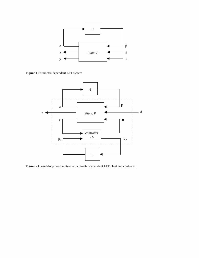
Figure 1 Parameter-dependent LFT system

Figure 2 Closed-loop combination of parameter-dependent LFT plant and controller

βα

d

u

e

y

Plant, P

θ

αKβK

βαd

u

e

y

Plant, P

θ

controller, K

θ