Survey of Polygonal Surface Simplification Algorithms

Paul S. Heckbert and Michael Garland

1 May 1997

School of Computer ScienceCarnegie Mellon University

Pittsburgh, PA 15213

Multiresolution Surface Modeling CourseSIGGRAPH ’97

This is a draft of a Carnegie Mellon University technical report, to appear. Seehttp://www.cs.cmu.edu/∼ph for final version.

Send comments or corrections to the authors at: fph,garlandg@cs.cmu.edu

Abstract

This paper surveys methods for simplifying and approximating polygonal surfaces. A polygonal surface is a piecewise-linear surface in 3-D defined by a set of polygons; typically a set of triangles. Methods from computer graphics, com-puter vision, cartography, computational geometry, and other fields are classified, summarized, and compared bothpractically and theoretically. The surface types range from height fields (bivariate functions), to manifolds, to non-manifold self-intersecting surfaces. Piecewise-linear curve simplification is also briefly surveyed.

This work was supported by ARPA contract F19628-93-C-0171 and NSF Young Investigator award CCR-9357763.

Keywords: multiresolution modeling, surface approx-imation, piecewise-linear surface, triangulated irregularnetwork, mesh coarsening, decimation, non-manifold,cartographic generalization, curve simplification, level ofdetail, greedy insertion.

Contents

1 Introduction 11.1 Characterizing Algorithms . . . . 21.2 Background on Application Areas 2

2 Curve Simplification 4

3 Surface Simplification 53.1 Height Fields and Parametric Sur-

faces . . . . . . . . . . . . . . . 63.2 Manifold Surfaces . . . . . . . . 163.3 Non-Manifold Surfaces . . . . . . 223.4 Related Techniques . . . . . . . . 23

4 Conclusions 23

5 Acknowledgements 23

6 References 24

1 Introduction

The simplification of surfaces has become increasinglyimportant as it has become possible in recent years to cre-ate models of greater and greater detail. Detailed sur-face models are generated in a number of disciplines. Forexample, in computer vision, range data is captured us-ing scanners; in scientific visualization, isosurfaces areextracted from volume data with the “marching cubes”algorithm; in remote sensing, terrain data is acquiredfrom satellite photographs; and in computer graphics andcomputer-aided geometric design, polygonal models aregenerated by subdivision of curved parametric surfaces.Each of these techniques can easily generate surface mod-els consisting of millions of polygons.

Simplification is useful in order to make storage, trans-mission, computation, and display more efficient. A com-pact approximation of a shape can reduce disk and mem-ory requirements and can speed network transmission. Itcan also accelerate a number of computations involvingshape information, such as finite element analysis, colli-sion detection, visibility testing, shape recognition, anddisplay. Reducing the number of polygons in a model canmake the difference between slow display and real time

display.

A variety of methods for simplifying curves and sur-faces have been explored over the years. Work on thistopic is spread among a number of fields, making literaturesearch quite challenging. These fields include: cartogra-phy, geographic information systems (GIS), virtual real-ity, computer vision, computer graphics, scientific visual-ization, computer-aided geometric design, finite elementmethods, approximation theory, and computational geom-etry.

Some prior surveys of related methods exist, notably abibliography on approximation [45], a survey of spatialdata structures for curves and surfaces [106], and surveysof triangulation methods with both theoretical [6] and sci-entific visualization [89] orientations. None of these sur-veys surface simplification in depth, however.

The present paper attempts to survey all previous workon surface simplification and place the algorithms in a tax-onomy. In this taxonomy, we intermix algorithms fromvarious fields, classifying algorithms not according to theapplication for which they were designed, but accordingto the technical problem they solve. By doing so, wefind great similarities between algorithms from disparatefields. For example, we find common ground betweenmethods for representing terrains developed in cartogra-phy, methods for approximating bivariate functions devel-oped in computational geometry and approximation the-ory, and methods for approximating range data developedin computer vision. This is not too surprising, since theseare fundamentally the same technical problem. By callingattention to these similarities, and to the past duplicationof work, we hope to facilitate cross-fertilization betweendisciplines.

Our emphasis is on methods that take polygonal sur-faces as input and produce polygonal surfaces as output,although we touch on curved parametric surface and vol-ume techniques. Our polygons will typically be planar tri-angles. Although surface simplification is our primary in-terest, we also discuss curve simplification, because manysurface methods are simple generalizations of curve meth-ods.

1

1.1 Characterizing Algorithms

Methods for simplifying curves and surfaces vary in theirgenerality and approach – among surface methods, someare limited to height fields, for example, while others areapplicable to general surfaces in 3-D. To systematize ourtaxonomy, we will classify methods according to the prob-lems that they solve and the algorithms they employ. Be-low is a list of the primary characteristics with which wewill do so:

Problem Characteristics

Topology and Geometry of Input: For curves, theinput can be a set of points, a function y(x), aplanar curve, or a space curve. For surfaces, theinput can be a set of points, samples of a heightfield z(x, y) in a regular grid or at scatteredpoints, a manifold1, a manifold with boundary,or a set of surfaces with arbitrary topology (e.g.a set of intersecting polygons).

Other Attributes of Input: Color, texture, and sur-face normals might be provided in addition togeometry.

Domain of Output Vertices: Vertices of the outputcan be restricted to be a subset of the inputpoints, or they can come from the continuousdomain.

Structure of Output Triangulation: Meshes canbe regular grids, they can come from a hier-archical subdivision such as a quadtree, orthey can be a general subdivision such as aDelaunay or data-dependent triangulation.

Approximating Elements: The approximatingcurve or surface elements can be piecewise-linear (polygonal), quadratic, cubic, highdegree polynomial, or some other basisfunction.

Error Metric: The error of the approximation istypically measured and minimized with respect

1A manifold is a surface for which the infinitesimal neighborhood ofevery point is topologically equivalent to a disk. In a triangulated mani-fold, each edge belongs to two triangles. In a triangulated manifold withboundary, each edge belongs to one or two triangles.

to L2 or L∞ error2. Distances can be measuredin various ways, e.g., to the closest point on agiven polygon, or closest point on the entire sur-face.

Constraints on Solution: One might request themost accurate approximation possible using agiven number of elements (e.g. line segmentsor triangles), or one might request the solu-tion using the minimum number of elementsthat satisfies a given error tolerance. Somealgorithms give neither type of guarantee, butgive the user only indirect control over thespeed/quality tradeoff. Other possible con-straints include limits on the time or memoryavailable.

Algorithm Characteristics

Speed/Quality Tradeoff: Algorithms that are opti-mal (minimal error and size) are typically slow,while algorithms that generate lower quality orless compact approximations can generally befaster.

Refinement/Decimation: Many algorithms canbe characterized as using either refinement, acoarse-to-fine approach starting with a minimalapproximation and building up more and moreaccurate ones, or decimation, a fine-to-coarseapproach starting with an exact fit, and dis-carding details to create less and less accurateapproximations.

1.2 Background on Application Areas

The motivations for surface simplification differ from fieldto field. Terminology differs as well.

2In this paper, we use the following error metrics: We define the L2

error between two n-vectors u and v as ||u−v||2 =[∑n

i=1(ui − vi )2]1/2

.The L∞ error, also called the maximum error, is ||u − v||∞ =maxn

i=1 |ui − vi|. We define the squared error to be the square of the L2error, and the root mean square or RMS error to be the L2 error dividedby√

n. Optimization with respect to the L2 and L∞ metrics are calledleast squares and minimax optimization, and we call such solutions L2–optimal and L∞–optimal, respectively.

2

Cartography. In cartography, simplification is onemethod among many for the “generalization” of geo-graphic information [86]. In that field, curve simplifica-tion is called “line generalization”. It is used to simplifythe representations of rivers, roads, coastlines, and otherfeatures when a map with large scale is produced. It isneeded for several reasons: to remove unnecessary detailfor aesthetic reasons, to save memory/disk space, and toreduce plotting/display time. The principal surface typesimplified in cartography is, of course, the terrain. Mapproduction was formerly a slow, off-line activity, but itis currently becoming more interactive, necessitating thedevelopment of better simplification algorithms.

The ideal error measures for cartographic simplificationinclude considerations of geometric error, viewer interest,and data semantics. Treatment of the latter issues is be-yond the scope of this study. The algorithms summarizedhere typically employ a geometric error measure based onEuclidean distance. The problem is thus to retain featureslarger than some size threshold, typically determined bythe limits of the viewer’s perception, the resolution of thedisplay device, or the available time or memory.

Computer Vision. Range data acquired by stereo orstructured light techniques (e.g. lasers) can easily producemillions of data points. It is desirable to simplify the sur-face models created from this data in order to remove re-dundancy, save space, and speed display and recognitiontasks. The acquired data is often noisy, so tolerance of andsmoothing of noise are important considerations here.

Computer Graphics. In computer graphics and theclosely related fields of virtual reality, computer-aided ge-ometric design, and scientific visualization, compact stor-age and fast display of shape information are vital. Forinteractive applications such as military flight simulators,video games, and computer-aided design, real time perfor-mance is a very important goal. For such applications, thegeometry can be simplified to multiple levels of detail, anddisplay can switch or blend between the appropriate lev-els of detail as a function of the screen size of each object[13, 52]. This technique is called multiresolution model-ing. Redisplaying a static scene from a moving viewpointis often called a walkthrough. For off-line, more realistic

simulations such as special effects in entertainment, realtime is not vital, but reasonable speed and storage are nev-ertheless important.

When 3-D shape models are transmitted, compression isvery important. This applies whether the channel has verylow bandwidth (e.g. a modem) or higher bandwidth (e.g.the Internet backbone). The rapid growth of the WorldWide Web is spurring some of the current work in surfacesimplification.

Finite Element Analysis. Engineers use the finite ele-ment method for structural analysis of bridges, to simulatethe air flow around airplanes, and to simulate electromag-netic fields, among other applications. A preprocess tosimulation is a “mesh generation” step. In 2-D mesh gen-eration, the domain, bounded by curves, is subdivided intotriangles or quadrilaterals. In 3-D mesh generation, the do-main is given by boundary surfaces. Surface meshes of tri-angles or quadrilaterals are first constructed, and then thevolume is subdivided into tetrahedra or hexahedra. Thecriteria for a good mesh include both geometric fidelityand considerations of the physical phenomena being simu-lated (stress, flow, etc). To speed simulation, it is desirableto make the mesh as coarse as possible while still resolvingthe physical features of interest. In 3-D simulations, sur-face details such as bolt heads might be eliminated, for ex-ample, before meshing the volume. This community callssimplification “mesh coarsening”.

Approximation Theory and Computational Geometry.What is called a terrain in cartography or a height field incomputer graphics is called a bivariate function or a func-tion of two variables in more theoretical fields. The goal inapproximation theory is often to characterize the error inthe limit as the mesh becomes infinitely fine. In compu-tational geometry the goal is typically to find algorithmsto generate approximations with optimal or near-optimalcompactness, error, or speed or to prove bounds on these.Implementation of algorithms and low level practical op-timizations receive less attention.

3

2 Curve Simplification

Curve simplification has been used in cartography, com-puter vision, computer graphics, and a number of otherfields.

A basic curve simplification problem is to take a poly-gonized curve with n vertices (a chain of line segments or“polyline”) as input and produce an approximating poly-gonized curve with m vertices as output. A closely relatedproblem is to take a curve with n vertices and approximateit within a specified error tolerance.

Douglas-Peucker Algorithm. The most widely usedhigh-quality curve simplification algorithm is probably theheuristic method commonly called the Douglas-Peucker3

algorithm. It was independently invented by many peo-ple [99], [31], [30, p. 338], [5, p. 92], [125], [91, p.176], [3]. At each step, the Douglas-Peucker algorithm at-tempts to approximate a sequence of points by a line seg-ment from the first point to the last point. The point far-thest from this line segment is found, and if the distanceis below threshold, the approximation is accepted, other-wise the algorithm is recursively applied to the two sub-sequences before and after the chosen point. This algo-rithm, though not optimal, has generally been found toproduce the highest subjective- and objective-quality ap-proximations when compared with many other heuristicalgorithms [85, 130]. Its best case time cost4 is �(n), itsworst case cost is O(mn), and its expected time cost isabout 2(n logm). The worst case behavior can be im-proved, with some sacrifice in the best case behavior, us-ing a2(n logn) algorithm employing convex hulls [54].

A variant of the Douglas-Peucker algorithm describedby Ballard and Brown [4, p. 234] on each iteration splitsat the point of highest error along the whole curve, insteadof splitting recursively. This yields higher quality approx-imations for slightly more time. If this subdivision tree is

3Pronounced, and later spelled, due to name change, “Poiker”.4A function is in O( f (n)) if it is less than or equal to c f (n) as n→∞,

for some positive constant c. “O” is used for upper bounds.A function is in2( f (n)) if it is between c1 f (n) and c2 f (n) as n→∞,for some positive constants c1, c2.A function is in�( f (n)) if it is greater than or equal to c f (n) as n→∞,for some positive constant c. “�” is used for lower bounds.

saved, it is possible to dynamically build an approximationfor any larger error tolerance very quickly [18].

A potential problem is that simplification can cause asimple polygon to become self-intersecting. This could bea problem in cartographic applications.

Faster or Higher Quality Algorithms. There are fasteralgorithms than Douglas-Peucker, but all of these aregenerally believed to have inferior quality [84]. Onesuch algorithm is the trivial method of regular subsam-pling (known as the “nth-point algorithm” in cartography),which simply keeps every kth point of the input, for somek, discarding the rest. This algorithm is very fast, but willsometimes yield very poor quality approximations.

Least squares techniques are commonly used for curvefitting in pattern recognition and computer vision, but theydo not appear to be widely used for that purpose in cartog-raphy.

Polygonal Boundary Reduction. While the Douglas-Peucker algorithm and its variants are refinement algo-rithms, curves can also be simplified using decimationmethods. Boxer et al. [8] describe two such algorithmsfor simplifying 2-D polygons. The first, due to Leu andChen [75], is a simple decimation algorithm. It considersboundary arcs of 2 and 3 edges. For each arc, it computesthe maximum distance between the arc and the chord con-necting its endpoints. It then selects an independent set ofarcs whose deviation is less than some threshold, and re-places them by their chords. The second algorithm is animprovement of this basic algorithm which guarantees thatthe approximate curve is always within some bounded dis-tance from the original. They state that the running time ofthe simple algorithm is 2(n), while the bounded-error al-gorithm requires O(n+ r2) time where r is the number ofvertices removed.

Optimal Approximations. Algorithms for optimalcurve simplification are much less common than heuristicmethods, probably because they are slower and/or morecomplicated to implement. In a common form of optimalcurve simplification, one searches for the approximationof a given size with minimum error, according to some

4

definition of “error”. Typically the output vertices arerestricted to be a subset of the input vertices. A naive,exhaustive algorithm would have exponential cost, sincethe number of subsets is exponential, but using dynamicprogramming and/or geometric properties, the cost can bereduced to polynomial. The L2–optimal approximationto a function y(x) can be found in O(mn2) time, worstcase, using dynamic programming. Remarkably, a slightvariation in the error metric permits a much faster algo-rithm: the L∞–optimal approximation to a function canbe found in O(n) time [63], using visibility techniques(see also [123, 91]). When the problem is generalizedfrom functions to planar curves, the complexity of the bestL∞–optimal algorithms we know of jumps to O(n2 log n)[63]. These methods use shortest-path graph algorithmsor convex hulls. For space curves (curves in 3-D), thereare O(n3 log m) L∞–optimal algorithms [62].

Asymptotic Approximation. In related work, McClureand de Boor analyzed the error when approximatinga highly continuous function y(x) using piecewise-polynomials with variable knots [82, 21]. We discussonly the special case of piecewise-linear approximations.They analyzed the asymptotic behavior of the Lp error ofapproximation in the limit as m, the number of vertices(knots) of the approximation, goes to infinity. Theyshowed that the asymptotic Lp error with regular subsam-pling is proportional to m−2, for any p. The Lp–optimalapproximation has the same asymptotic behavior, thoughwith a smaller constant. McClure showed that the spacingof vertices in the optimal approximation is closely re-lated to the function’s second derivative. Specifically, heproved that as m→∞, the density of vertices at each pointin the optimal L2 approximation becomes proportional to|y′′(x)|2/5. For optimal L∞ approximations, the density isproportional to |y′′(x)|1/2. Also, as m→∞, all intervalshave equal error in an Lp–optimal approximation.

The density property and the balanced error propertydescribed above can be used as the basis for curve sim-plification algorithms [82]. Although adherence to nei-ther property guarantees optimality for real simplificationproblems with finite m, iterative balanced error methodshave been shown to generate good approximations in prac-tice [91, p. 181]. Another caveat is that many curves in na-ture do not have continuous derivatives, but instead have

some fractal characteristics [80]. Nevertheless, these theo-retical results suggest the importance of the second deriva-tive, and hence curvature, in the simplification of curvesand surfaces.

Summary of Curve Simplification. The Douglas-Peucker algorithm is probably the most commonlyused curve simplification algorithm. Most implemen-tations have O(mn) cost, worst case, but typical costof 2(n logm). An optimization with worst case cost ofO(n logn) is available, however. Optimal simplificationtypically has quadratic or cubic cost, making it impracticalfor large inputs.

3 Surface Simplification

Surfaces are more difficult to simplify than curves. In theflight simulator field, lower level of detail models havetraditionally been prepared by hand [17]. The results canbe excellent, but the process can take weeks. Automaticmethods are preferable for large and dynamic databases,however.

If only a single level of detail is needed, then in somecases, simplification can be obviated by simply avoidinggeneration of redundant data in the first place. In scientificvisualization, for example, the marching cubes algorithm[90] is widely used. It generates many tiny triangles with-out testing for coplanarity between neighbors. A more so-phisticated alternative is adaptive polygonization that sub-divides finely only where the surface is highly curved [7].In computer aided geometric design, when polygonizingparametric surfaces, rather than subdivide and polygonizea surface with a regular (u, v) grid, better results are of-ten possible by subdividing adaptively based on curvature[10].

When simplification is needed however, one of the al-gorithms summarized below can be used.

Taxonomy of Surface Simplification Algorithms. Wecategorize algorithms at the highest level according to theclass of surfaces on which they operate:

• height fields and parametric surfaces,

5

• manifold surfaces, and

• non-manifold surfaces.

Within each surface class we often group algorithms ac-cording to whether they work by refinement or decima-tion. Within the subclasses, methods are generally listedchronologically. We have attempted to be fairly compre-hensive, so consequently the good methods are describedalong with the bad. As we summarize algorithms, welist their computational complexities and quote empiricaltimes, where known (of course, hardware, compilers, lan-guages, and programming styles differ between individu-als, so we must be careful when judging based on this in-formation). Complexities are given in terms of n, the num-ber of vertices in the input, and m, the number of verticesin the output. Typically, m� n.

3.1 Height Fields and Parametric Surfaces

Height fields and parametric surfaces are the simplestclass of surfaces. Within this class of surfaces, we dividemethods into the following six sub-classes: regular gridmethods, hierarchical subdivision methods, feature meth-ods, refinement methods, decimation methods, and opti-mal methods.

Regular grid methods are the simplest techniques, us-ing a grid of samples equally and periodically spaced inx and y. The hierarchical subdivision methods are basedon quadtree, k-d tree, and hierarchical triangulations us-ing a divide and conquer strategy. They recursively subdi-vide the surface into regions, constructing a tree-structuredhierarchy. The next four categories employ more generalsubdivision and triangulation methods, most commonlyDelaunay triangulation. Feature methods select a set ofimportant “feature” points in one pass and use them asthe vertex set for triangulation. Refinement methods areessentially generalizations of the Douglas-Peucker algo-rithm from curves to surfaces, where intervals are replacedby triangles and splitting is replaced by retriangulating.They start with a minimal approximation and use multiplepasses of point selection and retriangulation to build up thefinal triangulation. Decimation methods use an approachopposite that of refinement methods: they begin with a tri-angulation of all of the input points and iteratively delete

vertices from the triangulation, gradually simplifying theapproximation. Refinement methods thus work top-down,while decimation methods work bottom-up. The final cat-egory, “optimal methods” are distinguished more for theirtheoretical focus than for their method.

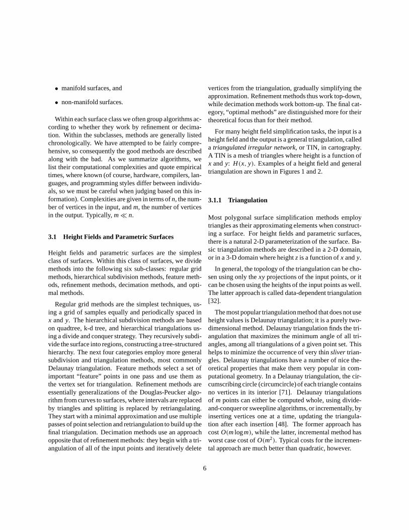
For many height field simplification tasks, the input is aheight field and the output is a general triangulation, calleda triangulated irregular network, or TIN, in cartography.A TIN is a mesh of triangles where height is a function ofx and y: H(x, y). Examples of a height field and generaltriangulation are shown in Figures 1 and 2.

3.1.1 Triangulation

Most polygonal surface simplification methods employtriangles as their approximating elements when construct-ing a surface. For height fields and parametric surfaces,there is a natural 2-D parameterization of the surface. Ba-sic triangulation methods are described in a 2-D domain,or in a 3-D domain where height z is a function of x and y.

In general, the topology of the triangulation can be cho-sen using only the xy projections of the input points, or itcan be chosen using the heights of the input points as well.The latter approach is called data-dependent triangulation[32].

The most popular triangulation method that does not useheight values is Delaunay triangulation; it is a purely two-dimensional method. Delaunay triangulation finds the tri-angulation that maximizes the minimum angle of all tri-angles, among all triangulations of a given point set. Thishelps to minimize the occurrence of very thin sliver trian-gles. Delaunay triangulations have a number of nice the-oretical properties that make them very popular in com-putational geometry. In a Delaunay triangulation, the cir-cumscribing circle (circumcircle) of each triangle containsno vertices in its interior [71]. Delaunay triangulationsof m points can either be computed whole, using divide-and-conqueror sweepline algorithms, or incrementally, byinserting vertices one at a time, updating the triangula-tion after each insertion [48]. The former approach hascost O(m logm), while the latter, incremental method hasworst case cost of O(m2). Typical costs for the incremen-tal approach are much better than quadratic, however.

6

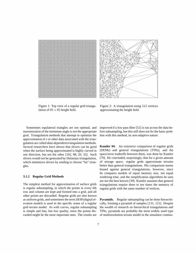
Figure 1: Top view of a regular grid triangu-lation of 65× 65 height field.

Figure 2: A triangulation using 512 verticesapproximating the height field.

Sometimes equilateral triangles are not optimal, andmaximization of the minimum angle is not the appropriategoal. Triangulation methods that attempt to optimize theapproximation of z or other data associated with the trian-gulation are called data-dependent triangulation methods.Several researchers have shown that slivers can be goodwhen the surface being approximated is highly curved inone direction, but not the other [102, 88, 20, 32]. Suchslivers would not be generated by Delaunay triangulation,which minimizes slivers by tending to choose “fat” trian-gles.

3.1.2 Regular Grid Methods

The simplest method for approximation of surface gridsis regular subsampling, in which the points in every kthrow and column are kept and formed into a grid, and allother points are discarded. Regular grids are also knownas uniform grids, and sometimes the term DEM (digital el-evation model) is used in the specific sense of a regulargrid terrain model. As with curves, regular subsamplingis simple and fast, but low quality, since the points dis-carded might be the most important ones. The results are

improved if a low pass filter [51] is run across the data be-fore subsampling, but this still does not fix the basic prob-lem with this method, its non-adaptive nature.

Kumler 94. An extensive comparison of regular grids(DEMs) and general triangulations (TINs), and thespace/error tradeoffs between them, was done by Kumler[70]. He concluded, surprisingly, that for a given amountof storage space, regular grids approximate terrainsbetter than general triangulations. His comparison seemsbiased against general triangulations, however, sincehe compares models of equal memory size, not equalrendering time, and the simplification algorithms he usesare not the best known [39]. Kumler assumes that generaltriangulations require three to ten times the memory ofregular grids with the same number of vertices.

Pyramids. Regular subsampling can be done hierarchi-cally, forming a pyramid of samples [131, 121]. Despitethe wealth of research on hierarchical triangulations andTINs, pyramids are probably the most widely used typeof multiresolution terrain model in the simulator commu-

7

nity [16, 17] and in the visualization/animation commu-nity [60], because of their simplicity and compactness.

3.1.3 Hierarchical Subdivision Methods

Hierarchical subdivision methods construct a triangula-tion by recursively subdividing a surface. They are theadaptive form of pyramids. The hierarchical pattern ofsubdivision, even if not stored explicitly in the data struc-ture, forms a tree, each node of which has no more than oneparent. With Delaunay triangulation and other general tri-angulation algorithms, the topology is not hierarchical, be-cause a triangle might have multiple parents. Hierarchicalsubdivision methods are generally fast, simple, and theyfacilitate multiresolution modeling. In perspective sceneswhere nearby portions of the terrain require more detailthan distant regions, the hierarchy facilitates rendering atadaptive levels of detail. Nearby portions are drawn at at afine level, while distant regions are drawn at a coarse level.The penalty for their simplicity and speed is that hierar-chical subdivision methods typically yield poorer qualityapproximations than more general triangulation methods.

Quadtrees and k-d Trees. Terrains and parametric sur-faces are easily simplified using adaptive quadtree and k-dtree subdivision methods [106, 105]. DeHaemer and Zydaused quadtree and k-d tree splitting at the point of max-imum error within each cell to approximate general 3-Dsurfaces described by a grid [27]. Taylor and Barrett de-scribed a similar method for terrains [122]. Von Herzenand Barr discuss a method for crack-free adaptive triangu-lation of parametric surfaces using quadtrees [128]. Gross,Gatti, and Staadt have used wavelets to construct quadtreeapproximations of height fields [44]. With an unoptimizedimplementation, they were able to simplify a 256×256 ter-rain in about 2 seconds on an SGI Indy.

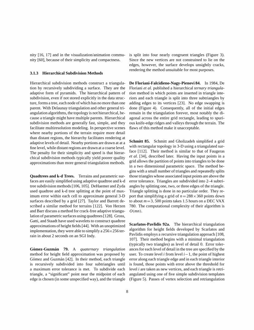
Gomez-Guzman 79. A quaternary triangulationmethod for height field approximation was proposed byGomez and Guzman [42]. In their method, each triangleis recursively subdivided into four subtriangles untila maximum error tolerance is met. To subdivide eachtriangle, a “significant” point near the midpoint of eachedge is chosen (in some unspecified way), and the triangle

is split into four nearly congruent triangles (Figure 3).Since the new vertices are not constrained to lie on theedges, however, the surface develops unsightly cracks,rendering the method unsuitable for most purposes.

De Floriani-Falcidieno-Nagy-Pienovi 84. In 1984, DeFloriani et al. published a hierarchical ternary triangula-tion method in which points are inserted in triangle inte-riors and each triangle is split into three subtriangles byadding edges to its vertices [23]. No edge swapping isdone (Figure 4). Consequently, all of the initial edgesremain in the triangulation forever, most notably the di-agonal across the entire grid rectangle, leading to spuri-ous knife-edge ridges and valleys through the terrain. Theflaws of this method make it unacceptable.

Schmitt 85. Schmitt and Gholizadeh simplified a gridwith rectangular topology in 3-D using a triangulated sur-face [112]. Their method is similar to that of Faugeraset al. [34], described later. Having the input points in agrid allows the partition of points into triangles to be donein a two dimensional parametric space. The method be-gins with a small number of triangles and repeatedly splitsthose triangles whose associated input points are above theerror tolerance. Triangles are subdivided into 2–4 subtri-angles by splitting one, two, or three edges of the triangle.Triangle splitting is done in no particular order. They re-port that simplifying a grid of n=288×360 points downto about m=3,500 points takes 1.5 hours on a DEC VAX780. The computational complexity of their algorithm isO(mn).

Scarlatos-Pavlidis 92a. The hierarchical triangulationalgorithm for height fields developed by Scarlatos andPavlidis employs a recursive triangulation approach [108,107]. Their method begins with a minimal triangulation(typically two triangles) as level of detail 0. Error toler-ances for each level of detail in the tree are specified by theuser. To create level i from level i−1, the point of highesterror along each triangle edge and in each triangle interioris found, those points with error above the threshold forlevel i are taken as new vertices, and each triangle is retri-angulated using one of five simple subdivision templates(Figure 5). Passes of vertex selection and retriangulation

8

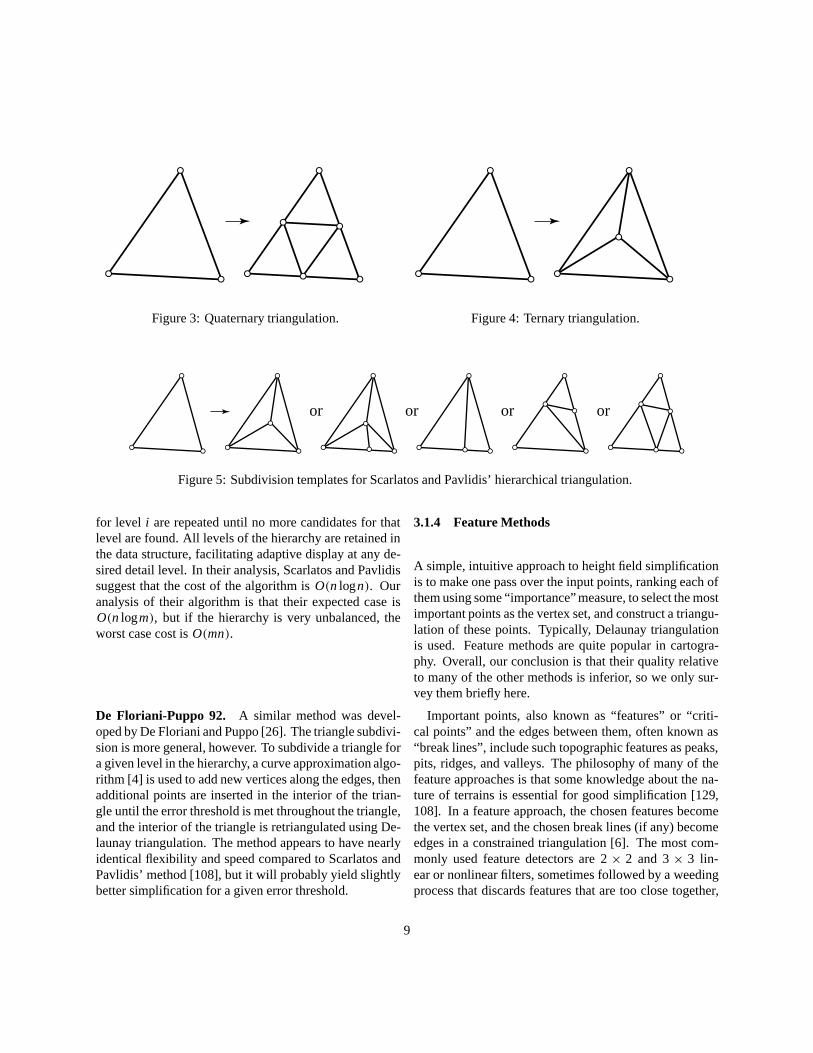
Figure 3: Quaternary triangulation. Figure 4: Ternary triangulation.

or or or or

Figure 5: Subdivision templates for Scarlatos and Pavlidis’ hierarchical triangulation.

for level i are repeated until no more candidates for thatlevel are found. All levels of the hierarchy are retained inthe data structure, facilitating adaptive display at any de-sired detail level. In their analysis, Scarlatos and Pavlidissuggest that the cost of the algorithm is O(n logn). Ouranalysis of their algorithm is that their expected case isO(n logm), but if the hierarchy is very unbalanced, theworst case cost is O(mn).

De Floriani-Puppo 92. A similar method was devel-oped by De Floriani and Puppo [26]. The triangle subdivi-sion is more general, however. To subdivide a triangle fora given level in the hierarchy, a curve approximation algo-rithm [4] is used to add new vertices along the edges, thenadditional points are inserted in the interior of the trian-gle until the error threshold is met throughout the triangle,and the interior of the triangle is retriangulated using De-launay triangulation. The method appears to have nearlyidentical flexibility and speed compared to Scarlatos andPavlidis’ method [108], but it will probably yield slightlybetter simplification for a given error threshold.

3.1.4 Feature Methods

A simple, intuitive approach to height field simplificationis to make one pass over the input points, ranking each ofthem using some “importance” measure, to select the mostimportant points as the vertex set, and construct a triangu-lation of these points. Typically, Delaunay triangulationis used. Feature methods are quite popular in cartogra-phy. Overall, our conclusion is that their quality relativeto many of the other methods is inferior, so we only sur-vey them briefly here.

Important points, also known as “features” or “criti-cal points” and the edges between them, often known as“break lines”, include such topographic features as peaks,pits, ridges, and valleys. The philosophy of many of thefeature approaches is that some knowledge about the na-ture of terrains is essential for good simplification [129,108]. In a feature approach, the chosen features becomethe vertex set, and the chosen break lines (if any) becomeedges in a constrained triangulation [6]. The most com-monly used feature detectors are 2 × 2 and 3 × 3 lin-ear or nonlinear filters, sometimes followed by a weedingprocess that discards features that are too close together,

9

such as a sequence of points along a ridge line. Such ap-proaches were employed by Peucker-Douglas and Chen-Guevara [92, 12]. Some methods examine larger neigh-borhoods of points in an attempt to measure importancemore globally.

Southard 91. One of the more interesting feature meth-ods is Southard’s [120]. He uses the Laplacian as a mea-sure of curvature. The rank of each point’s Laplacian iscomputed within a moving window, analogous to a me-dian filter in image processing, and all points whose rankis below some threshold are selected. This is an im-provement over the selection criteria of Peucker-Douglasand Chen-Guevara cited earlier, because it is less sus-ceptible to noise and high frequency variations, but un-fortunately, Southard’s ranking approach tends to dis-tribute points roughly uniformly across the domain, wast-ing points and leading to inferior approximations, in manycases. After computing the Delaunay triangulation of theselected points, Southard performs a data-dependent re-triangulation, swapping edges where that would reduce thesum of the absolute errors along the edges in the triangu-lation.

3.1.5 Refinement Methods

Refinement methods are multi-pass algorithms that beginwith a minimal initial approximation, on each pass theyinsert one or more points as vertices in the triangulation,and repeat until the desired error is achieved or the desirednumber of vertices is used. For input data in a rectangulargrid, the minimal approximation is two triangles; for othertopologies, the initial approximation might be more com-plex. Incremental methods are typically used to maintainthe triangulation as refinement proceeds.

To choose points, importance measures much like thoseof the feature methods can be used. Whereas feature meth-ods typically use importance measures that are indepen-dent of the approximation, in refinement algorithms, theimportance of a given point is usually a measure of theerror between it and the approximation. For a heightfield, the most common metric for the error is simplythe maximum absolute value of the vertical error, the L∞norm. This is the error measure most closely related to the

Douglas-Peucker algorithm.

Greedy Insertion. We call refinement algorithms thatinsert the point(s) of highest error on each pass greedy in-sertion algorithms, “greedy” because they make irrevoca-ble decisions as they go [15], and “insertion” because oneach pass they insert one or more vertices into the trian-gulation. Methods that insert a single point in each passwe call sequential greedy insertion and methods that in-sert multiple points in parallel on each pass we call paral-lel greedy insertion. The words “sequential” and “paral-lel” here refer to the selection and re-evaluation process,not to the architecture of the machine. Many variations onthe greedy insertion algorithm have been explored over theyears; apparently the algorithm has been reinvented manytimes.

Fowler-Little 79. In 1979, Fowler and Little publisheda hybrid algorithm that uses an initial pass of featureselection using 2 × 2 filters to “seed” the triangulation,followed by multiple passes of parallel greedy insertion[37]. On each of these latter passes, for each triangle, thepoint with highest error, or candidate point, is found, andall candidate points whose error is above the requestedthreshold are inserted into the triangulation. (When thepoint of highest error falls on an edge, they expand theirsearch for the candidate to a sector of the triangle’s circum-circle, a quirk unique to their algorithm.)

Fowler and Little discussed two methods for findingcandidates. In their exhaustive search method, the error ateach input point is computed and tested against the high-est error seen so far for that triangle. In the initial passesof a greedy insertion method, the triangles are big, neces-sitating the testing of many points, but in later passes thetriangles shrink and less testing per triangle is required.As a way to speed the selection of candidates, they pro-pose an alternative method using hill-climbing, in which atest point is initialized to the center of the triangle, and itrepeatedly steps to the neighboring input point of highesterror until it reaches a local maximum, where it becomesthe candidate. This latter method can be much faster, espe-cially for the initial passes, but it would also yield poorerquality approximations in many cases, because the hillclimbing might fail to find the global maximum within the

10

triangle. Unfortunately, Fowler and Little did not show acomparison of the results of the two methods, and did notanalyze the speed of their algorithm. An approach similarto Fowler and Little’s was very briefly described by Leeand Schachter [72].

De Floriani-Falcidieno-Pienovi 83. In 1983, De Flo-riani et al. presented a sequential greedy insertion algo-rithm [24, 25]. Their method is purer than Fowler andLittle’s: it does not seed the triangulation using featurepoints, and it inserts a single point on each pass, not multi-ple points. Consequently, the quality of its approximationscan be higher than Fowler and Little’s. The point insertedin each pass is the point of highest absolute error from theinput point set. To find this point they apparently visit allinput points on each pass, computing errors. Their papersays that their algorithm has worst case cost of O(n2), buttoo few details of the algorithm or its data structures areprovided to verify this. We will refer to this paper and al-gorithm as “DeFloriani83”.

De Floriani 89. In later work, De Floriani publishedan algorithm to build a “Delaunay pyramid” [22], a hier-archy of Delaunay triangulations, using a variant of her1983 greedy insertion algorithm to construct each levelof the pyramid. Her 1989 paper describes the greedy in-sertion algorithm in greater detail than her earlier papers([24, 25]).

Each triangle stores the set of input points it containsand the error of its candidate point. On each pass, the set oftriangles is scanned to find the candidate of highest error,this point is inserted using incremental Delaunay triangu-lation, and the candidates of all the triangles in the mod-ified region are recomputed. Recomputing the candidateof a triangle requires calculating the error at each point inthe triangle’s point set.

De Floriani states that the worst case time cost to createa complete pyramid of all n points is O(n2). We believethat the expected time cost of her algorithm, to select andtriangulate m points, is O(n logm+m2) (compare to Al-gorithm III in [40]).

Because point set traversal is used, rather than trianglescan conversion [36], this algorithm is not limited to input

points in a regular grid, as are most height field approxima-tion algorithms. The price of this generality is speed; theinner loops of a set traversal method cannot be optimizedas much as those of a scan conversion approach.

Heller 90. Heller explored a hybrid technique that hecalled “adaptive triangular mesh filtering” [53, p. 168].This technique is much like Fowler and Little’s. The prin-cipal difference is that the features are chosen not witha fixed-size local filter but by checking a variable-sizedneighborhood to determine if each point is a local ex-tremum within some height threshold. This feature selec-tion method, while more expensive than Fowler and Lit-tle’s, probably yields higher quality approximations.

His insertion method is sequential, like that of DeFlo-riani83. He optimizes the algorithm by storing the set ofcandidates, one candidate from each triangle, in a heap5.Below is an excerpt of Heller’s brief explanation of his al-gorithm [53, p. 168]:

The [insertion] of a point requires a local retrian-gulation which consists of swapping all neces-sary triangles, and readjusting the [importances]of all affected points. It is clear that the time forretriangulation is proportional to the number ofreadjusted points and the logarithm of the num-ber of queued points. It is, therefore, advisableto start the process with as many [feature] pointsas possible.

Due to his optimizations, Heller’s algorithm is probablyfaster than most others of comparable quality, such asDeFloriani83, but unfortunately, beyond the statementsquoted above he does not analyze the speed of his algo-rithm theoretically or empirically. It appears that the ex-pected complexity of the greedy insertion portion of hisalgorithm is O((m+n) logm), like Algorithm III in [40].

Schmitt-Chen 91. In order to segment computer visionrange data into planar regions, Schmitt and Chen use atwo stage process called split-and-merge [110, 91]. The

5Christoph Witzgall has also employed a heap. Personal communi-cation. 1994.

11

splitting stage is a form of greedy insertion with Delau-nay triangulation similar to DeFloriani83. The mergingstage joins together adjacent regions with similar normals,in the process destroying the triangulation, but yielding asegmentation of the image. Their splitting stage approxi-mated a height field with n=2562 points using about m=3,060 vertices in 67 seconds on a DEC VAX 8550.

Scarlatos-Pavlidis 92a and De Floriani-Puppo 92.The hierarchical triangulation methods of Scarlatos-Pavlidis [108] and De Floriani-Puppo [26] discussedearlier are analogous to greedy insertion in many ways,although their triangulations are quite different. Theirtechniques will typically use more triangles to achieve agiven error than sequential greedy insertion with Delau-nay triangulation, but on the other hand, they have theadvantage of a hierarchy.

Rippa 92. Rippa generalized the greedy insertion algo-rithm of DeFloriani83 to explore data-dependent triangu-lation and least squares fitting [101].

In place of incremental Delaunay triangulation, Rippa’salgorithm computes a data-dependent triangulation usinga version of Lawson’s local optimization procedure [71],repeatedly swapping edges around a new vertex until theglobal error reaches a local minimum. He tested two defi-nitions of global error. The first is a purely geometric mea-sure: the sum of the absolute values of the angles betweennormals of all pairs of adjacent triangles in the triangula-tion, and the second is a simple L2 measure: the sum ofsquares of absolute vertical errors over all input points.

From experiments with Delaunay and data-dependenttriangulation on several smooth, synthetic functions,Rippa concluded that data-dependent triangulation usu-ally yields more accurate approximations using a givennumber of vertices than Delaunay triangulation. Theangle criterion performed well in most cases, so he mildlyrecommended it over both the L2 criterion and Delaunaytriangulation. Rippa observed that the L2 criterion oc-casionally allowed long, extremely thin sliver trianglesthat did not fit the surface well to enter and remain inthe triangulation. The algorithm failed to eliminate suchtriangles because they were so thin that they contained noinput points, and hence they contributed zero error to the

L2 measure.

The angle criterion also made poor choices in somecases, so Rippa tried a hybrid scheme that on each passcompares the errors resulting from Delaunay triangula-tion and data-dependent triangulation with the angle crite-rion, and updates using the one with the smaller global er-ror. The hybrid scheme generated high quality approxima-tions more consistently than the other methods that Rippatested. Unfortunately, the hybrid is less elegant, and it ap-pears slower than the other methods. Margaliot and Gots-man reported an error measure yielding a better fit than theangle criterion [81].

Rippa also explored least squares methods that approx-imate the input points instead of interpolating them. The(x, y) coordinates of the vertices are frozen, but theirheights are allowed to vary, and the combination of heightsthat minimizes the global sum of squared errors is found.This involves solving a large, sparse, m×m system of lin-ear equations. He found that high quality results could beachieved fairly efficiently, on low-noise data, if the least-squares fitting was done as a post-process to greedy in-sertion. His empirical tests on simple functions showedthat least squares fitting roughly halved the error of thestandard interpolative methods. Overall, Rippa’s methodsappear expensive (data-dependent triangulation, particu-larly so) but the resulting approximations are higher qual-ity than those of simpler sequential greedy insertion meth-ods. The least squares technique appears to be particularlyeffective at improving the approximation.

Rippa tested his algorithm on rather small height fieldsand did not discuss computational costs of data-dependenttriangulation much.

Polis-McKeown 93. Polis and McKeown exploreda somewhat parallel variation of the greedy insertionmethod [95]. Their basic algorithm, in each pass, com-putes the absolute error at each input point. The set ofpoints of maximal absolute error is found, and these areinserted into the triangulation, one at a time, rejectingany that are within a tolerance distance of vertices al-ready in the triangulation (see paper for details). Thismethod might insert multiple points per triangle, unlikethe greedy insertion algorithms previously discussed. Itwould typically insert fewer points per pass than Fowler

12

and Little’s algorithm, however.

Several practical issues in the creation of large ter-rain models for simulators are raised by Polis and McK-eown. To facilitate dynamic loading of the terrain as aviewer roams, many display programs require that ter-rain databases be broken into small square blocks or “loadmodules”. This necessitates extra care along block bound-aries to avoid cracks between polygons. Polis and McKe-own also proposed selective fidelity, in which regions ofthe terrain could be assigned error weights according totheir visual importance, their likelihood of being seen, orsome other criterion. Thus, for example, for a tank simu-lator, one might weight navigable valleys more than inac-cessible mountain slopes.

Polis and McKeown tried a data-dependent triangu-lation method involving summing the squares of er-rors along all edges of the triangulation [94], much likeSouthard’s method. They found Delaunay triangulationto be preferable to data-dependent triangulation, however,because the former was much faster [95].

Polis and McKeown’s algorithm appears to have an ex-pected cost of O(mn) (like Algorithm I in [40]). They re-ported a compute time of 18 hours to select m= 76,500points total from an n=1,9792 terrain broken into 36 tileson a DECstation 5000. Speed was not the major issue forthem, however, since they were creating their TINs off-line. They later optimized their algorithm to select m=50,000 points from a terrain of n= 8,966,001 points in89 minutes on a DEC Alpha [93].

Franklin 93. Franklin has released code for a sequen-tial greedy insertion algorithm (PL/I code from 1973, Ccode from 1993) [38]. His algorithm is quite similar to De-Floriani83, but optimized in a manner similar to De Flo-riani’s Delaunay pyramid method ([22]). With each tri-angle, Franklin stores a candidate pointer, and he updatesonly the candidates of new or modified triangles on eachpass. He stores an array of input points with each triangle,as in [22], so the algorithm is more general but typicallyslower than a comparable surface simplification algorithmlimited to height fields.

Between his two implementations, Franklin has exper-imented with several triangulation methods: swapping an

edge if it reduces the maximum error of the approximation,swapping an edge if it has shorter length, and Delaunay tri-angulation.

Unfortunately, Franklin has not published his resultsand conclusions. By comparison to De Floriani’s De-launay pyramid algorithm and Algorithm III of [40], weconclude that the expected cost of Franklin’s algorithm isO(n logm+ m2). Franklin’s program can select m=100points from an n=2572 height field in 7 seconds on an SGIIndy.

Puppo-Davis-DeMenthon-Teng 94. Puppo et al. ex-plored terrain approximation algorithms for the Connec-tion Machine that are parallel both in the computer archi-tecture sense and also in the greedy insertion sense [98].Their algorithm is much like that of DeFloriani83, exceptthey insert all candidate points with error above the re-quested threshold on each pass, like Fowler and Little.They found that the number of points inserted on each passgrew exponentially, so the number of passes required toinsert m points would typically be2(log m). On a Think-ing Machines CM-2 with 16,384 processors, they reportedcompute times of 8 seconds to select m=379 points froman n=1282 terrain [98], or 86 seconds to select m=2,933points from an n=5122 terrain [97].

The algorithm was parallelized by assigning each in-put point to a different logical processor. Most of the par-allelization was straightforward, but parallel incrementaltriangulation required the use of special mutual exclusiontechniques to handle simultaneous topology changes inneighboring triangles.

Puppo et al. implemented both sequential and parallelgreedy insertion and concluded, surprisingly, that the latteris better. Our own experiments have indicated otherwise[40].

Chen-Schmitt 93. Chen and Schmitt explored a hybridfeature/refinement approach for triangulation of computervision range data [11]. To best approximate the step andslope discontinuities that are common in range data, theyfirst use edge detection to identify significant discontinu-ity features. These then become constraint curves duringgreedy insertion of additional vertices, using either con-

13

strained Delaunay or data-dependent triangulation. Chenand Schmitt found that data-dependent triangulation sim-plified better on surfaces with a preferred direction, suchas cylinders.

Silva-Mitchell-Kaufman 95. A rather different ap-proach to height field triangulation was proposed bySilva et al. [117]. We classify it here as a refinementmethod, although it is different in spirit from the previousmethods. Their method uses greedy cuts, triangulatingthe domain from the perimeter inward, on each pass“biting” out of the perimeter the triangle of largest areathat fits the input data within a specified maximum errortolerance. The method is thus a generalization of greedyvisibility techniques for curve simplification [123, 63],and also a form of data-dependent triangulation. In acomparison with Franklin’s greedy insertion algorithm,their unoptimized program was about two to four timesslower, but produced triangulations of a given qualityusing fewer vertices. They reported running times ofabout 8 seconds to select m=1,641 points from grids ofn=1202 points on a one-processor SGI Onyx.

Garland-Heckbert 95. Our own work in height fieldsimplification has explored fast and accurate variations ofthe greedy insertion algorithm [40, 39].

We explored two optimizations of the most basic greedyinsertion algorithm (as in DeFloriani83). First, we ex-ploited the locality of mesh changes, and only recalcu-lated the errors at input points for which the approxima-tion changed, and second, we used a heap to permit thepoint of highest error to be found more quickly. When ap-proximating an n point grid using an m vertex triangulatedmesh, these optimizations sped up the algorithm from anexpected time cost of O(mn) to O((m + n) logm). Wewere able to approximate an n=10242 grid to high qualityusing 1% of its points in about 21 seconds on a 150 MHzSGI Indigo2.

We also explored a data-dependent greedy insertiontechnique similar to Rippa’s method. We found an algo-rithm that yielded, in a fairly representative test, a solu-tion with 88% the error of Delaunay greedy insertion at acost of about 3–4 times greater. Source code for these al-gorithms is available.

In that paper, we propose several ideas for future workthat could improve the performance of the greedy inser-tion algorithm in the presence of cliff discontinuities, highfrequencies, and noise.

Arc/Info Latticetin. The geographic information sys-tem Arc/Info sold by the Environmental Systems ResearchInstitute (ESRI) can approximate terrain grids. Its “Lat-ticetin” command employs a hybrid feature/refinement ap-proach that starts with a regular grid of equilateral trian-gles and refines it with parallel greedy insertion [70, 95].

3.1.6 Decimation Methods

In contrast to refinement methods, the decimation ap-proach to surface simplification starts with the entire inputmodel and iteratively simplifies it, deleting vertices, trian-gles, or other geometric features on each pass. The deci-mation approach is not so common for height field simpli-fication; we will see far more decimation methods in thesection on manifold simplification.

Lee 89. A “drop heuristic” method for simplifying ter-rains was proposed by Lee [73]. We call it a vertex deci-mation approach because on each pass it deletes a vertex.The algorithm takes the height field grid as input and cre-ates an initial triangulation in which each 2× 2 square be-tween neighboring input points is split into two triangles[73]. On each pass, the error at each vertex is computedand the vertex with lowest error is deleted. The error at avertex is found by temporarily deleting the vertex from thetriangulation, doing a local Delaunay retriangulation, andmeasuring the vertical distance from the vertex to its con-taining triangle. The process continues until the error ex-ceeds the desired level, or the desired number of vertices isreached. Deletion in a Delaunay triangulation can be doneincrementally to avoid excessive cost [68].

The drop heuristic method yields high quality approx-imations, but its computational cost and memory cost ap-pear very high. When Lee compared his algorithm to Chenand Guevara’s method and to De Floriani’s ternary trian-gulation method [23], he found, not surprisingly, that hismethod yielded superior results [74]. The drop heuristic

14

method is expensive because of the need to visit each ver-tex on every pass. Its memory cost is high because a tri-angulation with n vertices must be created6.

Scarlatos-Pavlidis 92b. Scarlatos and Pavlidis exploreda method for adjusting a triangulation in order to equalizethe curvature of the input data within each triangle [109],extending McClure’s and Pavlidis’ earlier work [82, 91,83]. Their algorithm takes an initial triangulation and ap-plies three passes: shrinking triangles with high curvature,merging adjacent coplanar triangles, and swapping edgesto improve triangle shape and fit. In tests, the methodachieved little improvement when applied to the outputof their hierarchical triangulation algorithm [108, 107]: inmost cases, the method reduced the number of triangles,but it also increased the maximum error unless explicit er-ror tests were added [109]. Curvature equalization wasmore successful at improving regular subsampling meshes[107, p. 89]. No unshaded pictures of the resulting mesheswere given, however, so it is difficult to compare the qual-ity of the results to other methods.

Scarlatos 93. In addition to the recursive subdivisionmethod described earlier, Scarlatos also developed a ver-tex decimation method for constructing hierarchical trian-gulations [107]. The method begins with an initial trian-gulation and, to generate each level of the hierarchy, com-putes the “significance” of each vertex and deletes verticesin increasing order of significance until no more can bedeleted. Significance is an (unspecified) function of the er-ror between a vertex and a weighted average of its neigh-bors, and the degree of a vertex. The method is similar tothat of Schroeder et al., discussed later, except that Scar-latos’ method is limited to height fields, and it takes moreprecautions to minimize error accumulation. Scarlatos re-ported a running time of 7.75 minutes to build a completehierarchy for about n=5,900 points on a VAX 8530.

Hughes-Lastra-Saxe 96. The simplification algorithmdescribed by Hughes, Lastra, and Saxe [59] is targetedtowards simplifying global illumination meshes resulting

6We find that storing a triangulation with n vertices uses 5 to 100times the memory of a height field of n points because of the extra ad-jacency information required.

from radiosity systems. Consequently, the algorithm mustsimplify both the mesh geometry and the color values as-sociated with each mesh vertex. They rejected a greedy in-sertion algorithm because of its inability to deal well withsharp discontinuities (i.e., shadow borders). Instead, theychose a combination of local vertex decimation and sim-plification envelopes as in [126, 14]. Interestingly, theychose to select vertices for removal at random rather thanin order of increasing error. They claim that this providesmore uniform meshes, which they believe to be advan-tageous. Their method also uses higher-order elements(quadratic, cubic, etc.) for reconstructing the surface, apossibility which most simplification methods ignore.

3.1.7 Optimal Methods

The error of an optimal piecewise-linear, triangulated ap-proximation to a smooth function of two variables hasbeen analyzed in the limit as the number of triangles goesto infinity. Nadler showed that the L2–optimal approxima-tion has L2 error proportional to m−1 [88].

Finding the optimal approximation of a grid or surfaceusing triangulations of a subset of the input points could bedone by enumerating all possible subsets and all possibletriangulations, but this would take exponential time, andit would clearly be impractical. As with curves, certainproblems in optimal surface approximation are well under-stood, while others are not. It is known that L∞–optimalpolygonal approximation of convex surfaces is NP-hard(requires exponential time, in practice) [19, 9]. This im-plies, of course, that L∞–optimal approximation of heightfields and more general surfaces (in the space of all tri-angulations) is also NP-hard, since they are a superset ofconvex surfaces. We do not know if there are polyno-mial time algorithms for optimal surface simplification us-ing any other error metric (such as L2), or within a morerestricted class of triangulations. Even if some form ofthis problem permits an optimal algorithm with polyno-mial time, it would be surprising if it were as fast as theheuristic methods we have summarized above.

Polynomial time algorithms are known, however, forsub-optimal solutions with provable size and qualitybounds. If the optimal L∞ solution for a given errortolerance has mo vertices, there is an O(n7) algorithm

15

to find an approximation with the same error using m=O(mo log mo) vertices [87, 1], but this is far too slow to bepractical for large problems.

3.2 Manifold Surfaces

We now turn our attention from height fields and paramet-ric surfaces to manifolds and manifolds with boundary. Ingeneral, the manifold can have arbitrary genus and be non-orientable7 unless stated otherwise. Manifolds are moredifficult to simplify than height fields or parametric sur-faces because there is no natural 2-D parameterization ofthe surface. Delaunay triangulation is thus less easily ap-plied. We group manifold simplification methods into twoclasses: refinement methods and decimation methods.

3.2.1 Refinement Methods

Faugeras-Hebert-Mussi-Boissonnat 84. Faugeraset al. developed a technique somewhat similar to DeFloriani’s 1984 algorithm, but it does not have persistentlong edges, and it is applicable to the simplification of any3-D triangulated mesh of genus 0, not just height fields[34]. The method begins with a pancake-like two-triangleapproximation defined by three vertices of the input mesh.Associated with each triangle of the approximation is aset of input points. In successive passes, for each triangleof the approximation, the input point farthest from thetriangle is found, and if the distance is above threshold,the triangle is split into 3–6 subtriangles by insertingnew vertices at the interior point of highest error. Edgescommon to two subdivided triangles are split at theirpoints of highest error (Figure 6). Splitting in this wayeliminates the long edges of ternary triangulation.

During subdivision, each triangle’s point set must bepartitioned into 3–6 subsets. In methods that are limited toheight fields, the partition of input points to subtriangles isdone with simple projection and linear splitting. To parti-tion point sets on a surface in 3-D, Faugeras et al. insteadsplit using the shortest path along edges of the input mesh.

7A manifold is orientable if its two sides can be consistently labeledas “inside” and “outside”. A Mobius strip is non-orientable.

The method simplified an n= 2,000 point model in 1minute on a Perkin Elmer computer. The approximationsgenerated were sometimes poor, however, and the methodhad particular problems with concavities [96]. A later sub-division data structure, the “prism tree”, addressed theseproblems by recursively subdividing surface points intotruncated pyramidal volumes [96].

Delingette 94. A related method for the simplificationof orientable manifolds was developed by Delingette [28].He fits surfaces to sets of 3-D points by minimizing an en-ergy function which is a sum of an error term, an edgelength term, and a curvature term. The algorithm startswith a mesh that is the dual to a subdivided icosahedron.It then iteratively adjusts the geometry, attempting to min-imize the global energy [29]. After a good initial fit isachieved with this fixed topology, the mesh is refined. Re-gions of the mesh with high curvature, high local fit er-ror, or elongated faces are subdivided and vertices migrateto points of high curvature [28]. Delingette reports that ittakes 2 to 7 minutes to approximate a set of n=260,000points with a mesh of m= 1,700 vertices on a DEC Al-pha. The method is much faster than the related methodof Hoppe et al. [58], but it does not achieve comparablesimplification, and it has a number of parameters that ap-pear to require careful tuning.

Lounsbery-Eck-et al. 95. A two-stage method for mul-tiresolution wavelet modeling of arbitrary triangulatedpolyhedra was developed by Lounsbery, Eck, et al. [76,33]. The method is not limited to height fields or even totriangulated meshes with spherical topology; it can be ap-plied to any triangulated manifold with boundary. The ap-proach first constructs a base mesh which is a triangulatedpolyhedron with the same topology as the input surface.Geodesic-like distance measures are used in this step, rem-iniscent of the method of Faugeras et al.. It then uses re-peated quaternary subdivision of the base mesh to con-struct a new mesh that approximates the input surface veryclosely. A multiresolution model of the new mesh is thenbuilt using wavelet techniques, after which an approxima-tion at any desired error tolerance can be quickly gener-ated. Eck et al. simplified a model with about n=35,000vertices to m=5,400 vertices in 22 minutes of resampling

16

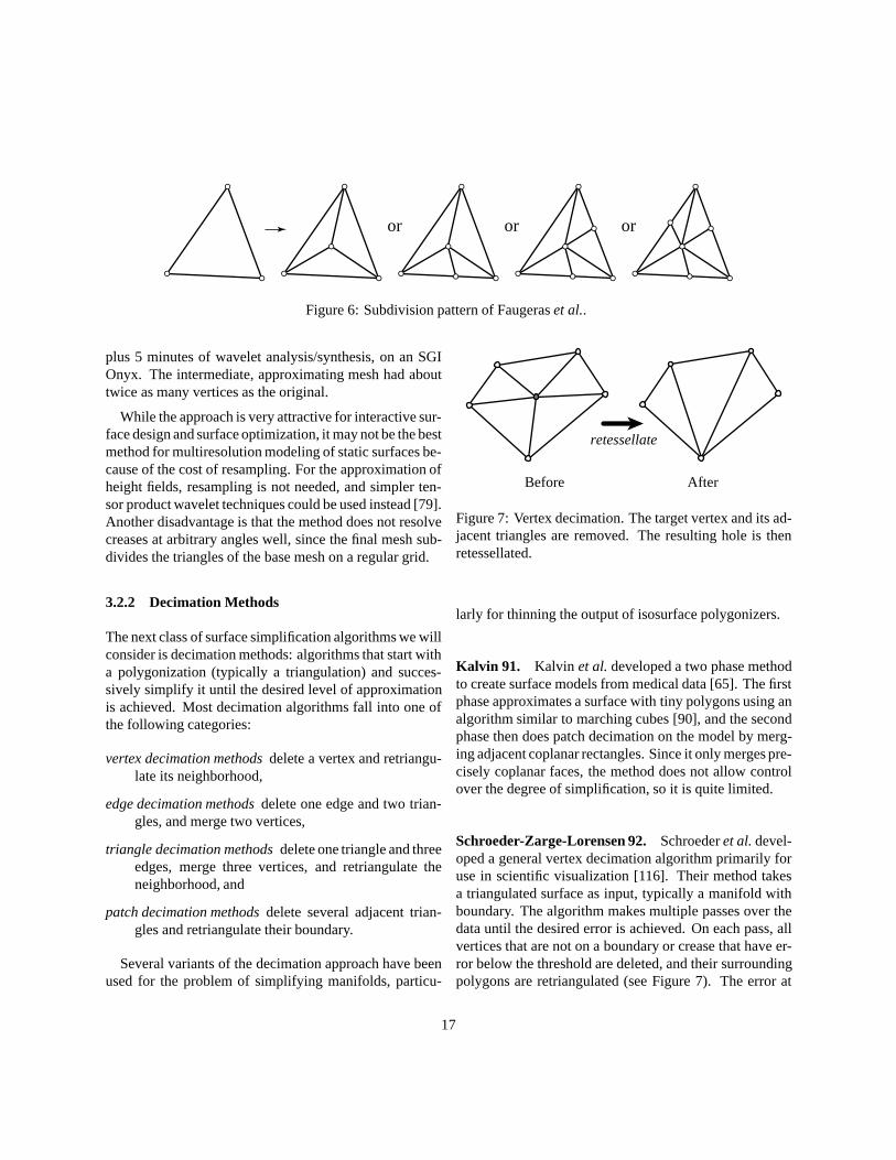
or or or

Figure 6: Subdivision pattern of Faugeras et al..

plus 5 minutes of wavelet analysis/synthesis, on an SGIOnyx. The intermediate, approximating mesh had abouttwice as many vertices as the original.

While the approach is very attractive for interactive sur-face design and surface optimization, it may not be the bestmethod for multiresolution modeling of static surfaces be-cause of the cost of resampling. For the approximation ofheight fields, resampling is not needed, and simpler ten-sor product wavelet techniques could be used instead [79].Another disadvantage is that the method does not resolvecreases at arbitrary angles well, since the final mesh sub-divides the triangles of the base mesh on a regular grid.

3.2.2 Decimation Methods

The next class of surface simplification algorithms we willconsider is decimation methods: algorithms that start witha polygonization (typically a triangulation) and succes-sively simplify it until the desired level of approximationis achieved. Most decimation algorithms fall into one ofthe following categories:

vertex decimation methods delete a vertex and retriangu-late its neighborhood,

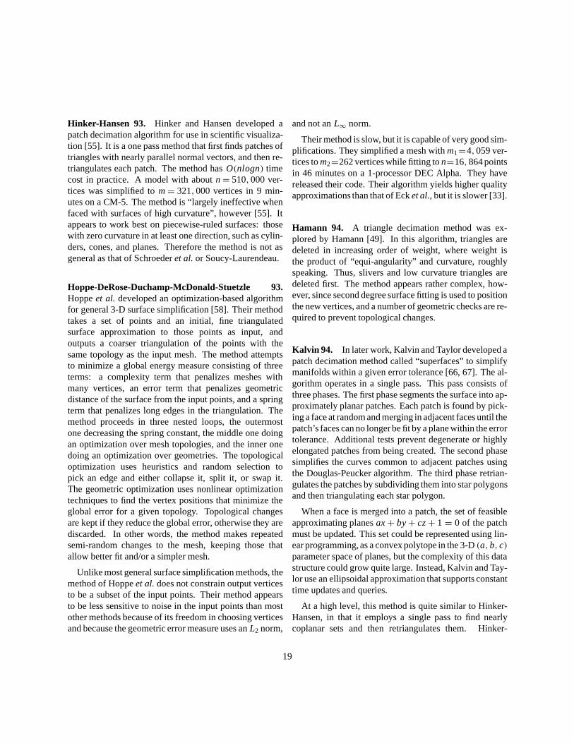
edge decimation methods delete one edge and two trian-gles, and merge two vertices,

triangle decimation methods delete one triangle and threeedges, merge three vertices, and retriangulate theneighborhood, and

patch decimation methods delete several adjacent trian-gles and retriangulate their boundary.

Several variants of the decimation approach have beenused for the problem of simplifying manifolds, particu-

retessellate

Before After

Figure 7: Vertex decimation. The target vertex and its ad-jacent triangles are removed. The resulting hole is thenretessellated.

larly for thinning the output of isosurface polygonizers.

Kalvin 91. Kalvin et al. developed a two phase methodto create surface models from medical data [65]. The firstphase approximates a surface with tiny polygons using analgorithm similar to marching cubes [90], and the secondphase then does patch decimation on the model by merg-ing adjacent coplanar rectangles. Since it only merges pre-cisely coplanar faces, the method does not allow controlover the degree of simplification, so it is quite limited.

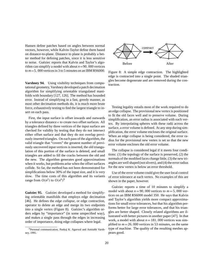
Schroeder-Zarge-Lorensen 92. Schroeder et al. devel-oped a general vertex decimation algorithm primarily foruse in scientific visualization [116]. Their method takesa triangulated surface as input, typically a manifold withboundary. The algorithm makes multiple passes over thedata until the desired error is achieved. On each pass, allvertices that are not on a boundary or crease that have er-ror below the threshold are deleted, and their surroundingpolygons are retriangulated (see Figure 7). The error at

17

a vertex is the distance from the point to the approximat-ing plane of the surrounding vertices. Note that errors aremeasured with respect to the previous approximation, notrelative to the input points, so errors can accumulate (thisflaw was fixed in later versions of the algorithm). Theirpaper demonstrated simplifications of models containingas many as 1,700,000 triangles. The computation time tosimplify a model of n= 400,000 vertices to m= 40,000vertices is about 14 minutes on an R4000 processor [115].This method uses significant memory, like Lee’s. To con-serve memory, compact data structures were developed[115]. Source code for this algorithm is available [114].

Relative to Lee’s method, the technique of Schroeder etal. is more general since it is not limited to height fields,it uses a less expensive and less accurate error measure,and it deletes multiple vertices per pass. Consequently, itis faster, but probably has lower quality.

Soucy and Laurendeau 92. To simplify manifolds withboundary, Soucy and Laurendeau also developed a vertexdecimation algorithm [118, 119]. Their application wasthe construction of surface models from multiple rangeviews. On each pass, the vertex with least error is deleted,and its neighborhood (the set of adjacent triangles) isretriangulated. The process stops when the error risesabove a specified tolerance or the desired size of model isachieved.

To compute rigorous error bounds, a set of deleted ver-tices is stored with each triangle. We will call these pointsthe ancestors of the triangle. To compute the error at avertex, a temporary vertex deletion and retriangulation aredone. The error of a vertex is a measure of the error thatwould result from its removal. More precisely, it is de-fined to be the maximum distance between either an an-cestor from the neighborhood or the vertex itself to the re-triangulated surface. Deletion of a non-boundary vertex isconsidered legal if the neighborhood triangles can be pro-jected to 2-D without foldover.

To retriangulate, Soucy and Laurendeau first computea constrained Delaunay triangulation in a 2-D projection,then this triangulation is improved using a version of Law-son’s local optimization procedure [71] adapted to sur-faces in 3-D. To update the data structures after retriangu-lation, first the ancestor lists are redistributed among the

new triangles, then the error of each formerly neighboringvertex is updated.

We can relate the method to several of its precursors.Like Lee’s method, this algorithm does vertex decimationby “one move lookahead”, but unlike his technique, it isnot limited to height fields. Like Faugeras et al. and DeFloriani et al. (1989), it stores a point set with each trian-gle, but unlike those methods, it is a decimation algorithm,and it is more general: it can simplify any manifold withboundary.

Soucy and Laurendeau estimate the expected complex-

ity of their algorithm to be O(

n log (n/(n−m)))

. Their

method appears to yield higher quality results than themethod of Schroeder et al., but it is slower and it uses morememory, since it maintains lists of all deleted points. A re-vised version of this algorithm is used in the IMCompresssoftware sold by InnovMetric [64].

Turk 92. Another method for simplifying a manifoldwith boundary is due to Turk [124]. This algorithm is nota decimation method in the same sense as the previousmethods, but we list it here because it also starts with a fulltriangulation and simplifies.

Turk’s algorithm takes a triangulated surface as input,sprinkles a user-specified number of points on these tri-angles at random, and uses an iterative repulsion proce-dure to spread the points out nearly uniformly. The pointsremain on the surface as they move about. After thesepoints are inserted into the original surface triangulation,the original vertices are deleted one by one, yielding a tri-angulation of the new vertices that has the same topologyas the original surface. Turk also demonstrated an im-proved variant of this technique that groups points mostdensely where the surface is highly curved.

Turk’s method appears to be best for smooth surfaces,since it tends to blur sharp features8. Overall, it appearsthat Turk’s algorithm is quite complex and that it will yieldresults inferior in quality to the methods of Schroeder et al.or Soucy-Laurendeau.

8William Schroeder, SIGGRAPH ’94 tutorial talk.

18

Hinker-Hansen 93. Hinker and Hansen developed apatch decimation algorithm for use in scientific visualiza-tion [55]. It is a one pass method that first finds patches oftriangles with nearly parallel normal vectors, and then re-triangulates each patch. The method has O(nlogn) timecost in practice. A model with about n= 510,000 ver-tices was simplified to m = 321,000 vertices in 9 min-utes on a CM-5. The method is “largely ineffective whenfaced with surfaces of high curvature”, however [55]. Itappears to work best on piecewise-ruled surfaces: thosewith zero curvature in at least one direction, such as cylin-ders, cones, and planes. Therefore the method is not asgeneral as that of Schroeder et al. or Soucy-Laurendeau.

Hoppe-DeRose-Duchamp-McDonald-Stuetzle 93.Hoppe et al. developed an optimization-based algorithmfor general 3-D surface simplification [58]. Their methodtakes a set of points and an initial, fine triangulatedsurface approximation to those points as input, andoutputs a coarser triangulation of the points with thesame topology as the input mesh. The method attemptsto minimize a global energy measure consisting of threeterms: a complexity term that penalizes meshes withmany vertices, an error term that penalizes geometricdistance of the surface from the input points, and a springterm that penalizes long edges in the triangulation. Themethod proceeds in three nested loops, the outermostone decreasing the spring constant, the middle one doingan optimization over mesh topologies, and the inner onedoing an optimization over geometries. The topologicaloptimization uses heuristics and random selection topick an edge and either collapse it, split it, or swap it.The geometric optimization uses nonlinear optimizationtechniques to find the vertex positions that minimize theglobal error for a given topology. Topological changesare kept if they reduce the global error, otherwise they arediscarded. In other words, the method makes repeatedsemi-random changes to the mesh, keeping those thatallow better fit and/or a simpler mesh.

Unlike most general surface simplification methods, themethod of Hoppe et al. does not constrain output verticesto be a subset of the input points. Their method appearsto be less sensitive to noise in the input points than mostother methods because of its freedom in choosing verticesand because the geometric error measure uses an L2 norm,

and not an L∞ norm.

Their method is slow, but it is capable of very good sim-plifications. They simplified a mesh with m1=4,059 ver-tices to m2=262 vertices while fitting to n=16,864 pointsin 46 minutes on a 1-processor DEC Alpha. They havereleased their code. Their algorithm yields higher qualityapproximations than that of Eck et al., but it is slower [33].

Hamann 94. A triangle decimation method was ex-plored by Hamann [49]. In this algorithm, triangles aredeleted in increasing order of weight, where weight isthe product of “equi-angularity” and curvature, roughlyspeaking. Thus, slivers and low curvature triangles aredeleted first. The method appears rather complex, how-ever, since second degree surface fitting is used to positionthe new vertices, and a number of geometric checks are re-quired to prevent topological changes.

Kalvin 94. In later work, Kalvin and Taylor developed apatch decimation method called “superfaces” to simplifymanifolds within a given error tolerance [66, 67]. The al-gorithm operates in a single pass. This pass consists ofthree phases. The first phase segments the surface into ap-proximately planar patches. Each patch is found by pick-ing a face at random and merging in adjacent faces until thepatch’s faces can no longer be fit by a plane within the errortolerance. Additional tests prevent degenerate or highlyelongated patches from being created. The second phasesimplifies the curves common to adjacent patches usingthe Douglas-Peucker algorithm. The third phase retrian-gulates the patches by subdividing them into star polygonsand then triangulating each star polygon.

When a face is merged into a patch, the set of feasibleapproximating planes ax+ by+ cz + 1 = 0 of the patchmust be updated. This set could be represented using lin-ear programming, as a convex polytope in the 3-D (a, b, c)parameter space of planes, but the complexity of this datastructure could grow quite large. Instead, Kalvin and Tay-lor use an ellipsoidal approximation that supports constanttime updates and queries.

At a high level, this method is quite similar to Hinker-Hansen, in that it employs a single pass to find nearlycoplanar sets and then retriangulates them. Hinker-

19

Hansen define patches based on angles between normalvectors, however, while Kalvin-Taylor define them basedon distance-to-plane. Distance to plane is probably a bet-ter method for defining patches, since it is less sensitiveto noise. Gueziec reports that Kalvin and Taylor’s algo-rithm can simplify a model with about n=90,000 verticesto m=5,000 vertices in 3 to 5 minutes on an IBM RS6000.

Varshney 94. Using visibility techniques from compu-tational geometry, Varshney developed a patch decimationalgorithm for simplifying orientable triangulated mani-folds with boundary [127, 126]. The method has boundederror. Instead of simplifying in a fast, greedy manner, asmost other decimation methods do, it is much more bruteforce, exhaustively testing to find the largest triangle to in-sert on each pass.

First, the input surface is offset inwards and outwardsby a tolerance distance ε to create two offset surfaces. Alltriangles defined by three vertices of the input surface arechecked for validity by testing that they do not intersecteither offset surface and that they do not overlap previ-ously inserted triangles. On each pass of the algorithm, thevalid triangle that “covers” the greatest number of previ-ously uncovered input vertices is inserted, the old triangu-lation of this portion of the surface is deleted, and smalltriangles are added to fill the cracks between the old andthe new. The algorithm generates good approximationswhen it works, but problems arise when the offset surfacescollide. So far, the method has not been demonstrated forsimplifications below 30% of the input size, and it is veryslow. The time costs of this algorithm and its variantsrange from O(n2) to O(n6)9

Gueziec 95. Gueziec developed a method for simplify-ing orientable manifolds that employs edge decimation[46]. He defines the edge collapse, or edge contraction,operator to delete an edge and merge its two endpointsinto a single vertex (Figure 8). Gueziec’s algorithm or-ders edges by “importance” (in some unspecified way),and makes a single pass through the edges in increasingorder of importance, doing edge collapses where legal.

9Personal communication, Pankaj K. Agarwal and Amitabh Varsh-ney, 1995.

Before After

contract

Figure 8: A simple edge contraction. The highlightededge is contracted into a single point. The shaded trian-gles become degenerate and are removed during the con-traction.

Testing legality entails most of the work required to doan edge collapse. The provisional new vertex is positionedto fit the old faces well and to preserve volume. Duringsimplification, an error radius is associated with each ver-tex. By interpolating spheres with these radii across thesurface, a error volume is defined. At any step during sim-plification, the error volume encloses the original surface.When an edge collapse is being considered, the error ra-dius for the provisional new vertex is set so that the newerror volume encloses the old error volume.

The collapse is considered legal if it meets four condi-tions: (1) the topology of the surface is preserved, (2) thenormals of the modified faces change little, (3) the new tri-angles are well shaped (not slivers), and (4) the error radiusfor the new vertex is below an error threshold.

Use of the error volume could give the user local controlof error tolerance at each vertex. No examples of this areshown in the paper, however.

Gueziec reports a time of 10 minutes to simplify amodel with about n= 90,000 vertices to m= 5,000 ver-tices on an IBM RS6000 model 350. He says that Kalvinand Taylor’s algorithm yields more compact approxima-tions for small error tolerances, but that his algorithm per-forms better for large error tolerances, and that his trian-gles are better shaped. Closely related algorithms are il-lustrated with better pictures in another paper [47]. In thatwork, a model with about n=181,000 vertices was sim-plified to m=26,000 vertices in 53 minutes, on the sametype of machine. The quality of the resulting meshes ap-pears good.

20

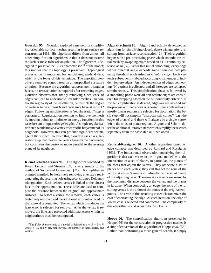
Gourdon 95. Gourdon explored a method for simplify-ing orientable surface meshes resulting from surface re-construction [43]. His algorithm differs from almost allother simplification algorithms in that it does not assumethe surface mesh to be a triangulation. The algorithm is de-signed to preserve the Euler characteristic10 of the model;this implies that the topology is preserved. Topologicalpreservation is important for simplifying medical data,which is the focus of this technique. The algorithm iter-atively removes edges based on an unspecified curvaturecriterion. Because the algorithm supports non-triangularfacets, no retessellation is required after removing edges.Gourdon observes that simply removing a sequence ofedges can lead to undesirable, irregular meshes. To con-trol the regularity of the tessellation, he restricts the degreeof vertices to be at most 6 and facet may have at most 12edges. Following simplification, a “regularization” step isperformed. Regularization attempts to improve the meshby moving points to minimize an energy function, in thiscase the sum of squared edge lengths. A simple regulariza-tion step would move a vertex towards the barycenter of itsneighbors. However, this can produce significant shrink-age of the surface. To avoid this, Gourdon uses a regular-ization step that moves the vertex towards the barycenter,but constrains the vertex to move parallel to the averageplane of its neighbors.

Klein-Liebich-Strasser 96. The algorithm described byKlein, Liebich, and Strasser [69] is very similar to themethod of Soucy and Laurendeau [119]. It simplifies anoriented manifold by iteratively removing a vertex a retri-angulating the resulting hole using a constrained Delaunaytriangulation. Each deleted vertex is linked to the closestface in the approximation. These links are used to com-pute the distance between the original and approximatesurfaces. To select a vertex for removal, each vertex istentatively removed and the additional error introduced bythe removal is computed. The vertex which introduces theleast error is selected for removal. After the vertex is re-moved, the links and projected additional errors within itsneighborhood must be recomputed.

10The Euler characteristic of a model is defined as χ = F − E + Vwhere F, E, and V are, respectively, the number of faces, edges, andvertices.

Algorri-Schmitt 96. Algorri and Schmitt developed analgorithm for simplifying closed, dense triangulations re-sulting from surface reconstruction [2]. Their algorithmbegins with a pre-processing phase which smooths the ini-tial mesh by swapping edges based on a G1-continuity cri-terion as in [32]. After this initial smoothing, every edgewhose dihedral angle exceeds some user-specified pla-narity threshold is classified as a feature edge. Each ver-tex is subsequently labeled according to its number of inci-dent feature edges. An independent set of edges connect-ing “0” vertices is collected, and all the edges are collapsedsimultaneously. This simplification phase is followed bya smoothing phase were all non-feature edges are consid-ered for swapping based on the G1-continuity criterion. Iffurther simplification is desired, edges are reclassified andthe process outlined above is repeated. Since only edges inmostly planar regions are selected for decimation, the ba-sic step will not simplify “characteristic curves” (e.g., theedges of a cube) and there will always be a single vertexleft in the midst of planar regions. Algorri and Schmitt de-scribe additional iterative steps which simplify these casesseparately from the basic step outlined above.

Ronfard-Rossignac 96. Another algorithm based onedge collapse was described by Ronfard and Rossignac[103]. The fundamental observation underlying their al-gorithm is that each vertex in the original model lies at theintersection of a set of planes, in particular, the planes ofthe faces that adjoin the vertex. They associate a set ofplanes with each vertex; they call this set the zone of thevertex. A vertex’s zone is initialized to be the set of planesof the adjoining faces. The error at a vertex is measured bythe maximum distance between the vertex and the planesin its zone. When contracting an edge, the zone of the re-sulting vertex is the union of the zones of the original end-points. The error of this resulting vertex characterizes thecost of contracting the edge. At each iteration, the edge oflowest cost is selected and contracted. The complexity ofthis algorithm would seem to be O(n logn).

Hoppe 96. The simplification algorithm presented byHoppe [56] for the construction of progressive meshes isa simplified version of the algorithm of Hoppe et al. [58].Rather than performing a more general search, it simply

21

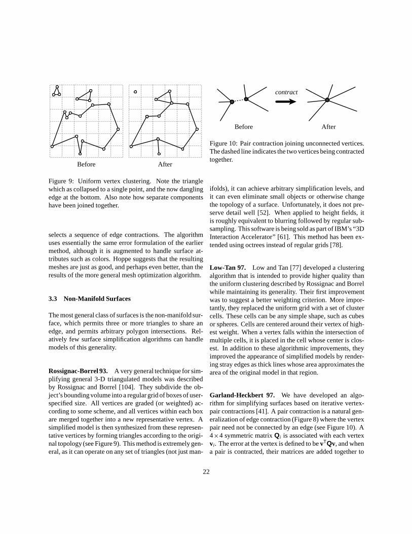
Before After

Figure 9: Uniform vertex clustering. Note the trianglewhich as collapsed to a single point, and the now danglingedge at the bottom. Also note how separate componentshave been joined together.

selects a sequence of edge contractions. The algorithmuses essentially the same error formulation of the earliermethod, although it is augmented to handle surface at-tributes such as colors. Hoppe suggests that the resultingmeshes are just as good, and perhaps even better, than theresults of the more general mesh optimization algorithm.

3.3 Non-Manifold Surfaces

The most general class of surfaces is the non-manifold sur-face, which permits three or more triangles to share anedge, and permits arbitrary polygon intersections. Rel-atively few surface simplification algorithms can handlemodels of this generality.

Rossignac-Borrel 93. A very general technique for sim-plifying general 3-D triangulated models was describedby Rossignac and Borrel [104]. They subdivide the ob-ject’s bounding volume into a regular grid of boxes of user-specified size. All vertices are graded (or weighted) ac-cording to some scheme, and all vertices within each boxare merged together into a new representative vertex. Asimplified model is then synthesized from these represen-tative vertices by forming triangles according to the origi-nal topology (see Figure 9). This method is extremely gen-eral, as it can operate on any set of triangles (not just man-

contract

Before After

Figure 10: Pair contraction joining unconnected vertices.The dashed line indicates the two vertices being contractedtogether.

ifolds), it can achieve arbitrary simplification levels, andit can even eliminate small objects or otherwise changethe topology of a surface. Unfortunately, it does not pre-serve detail well [52]. When applied to height fields, itis roughly equivalent to blurring followed by regular sub-sampling. This software is being sold as part of IBM’s “3DInteraction Accelerator” [61]. This method has been ex-tended using octrees instead of regular grids [78].

Low-Tan 97. Low and Tan [77] developed a clusteringalgorithm that is intended to provide higher quality thanthe uniform clustering described by Rossignac and Borrelwhile maintaining its generality. Their first improvementwas to suggest a better weighting criterion. More impor-tantly, they replaced the uniform grid with a set of clustercells. These cells can be any simple shape, such as cubesor spheres. Cells are centered around their vertex of high-est weight. When a vertex falls within the intersection ofmultiple cells, it is placed in the cell whose center is clos-est. In addition to these algorithmic improvements, theyimproved the appearance of simplified models by render-ing stray edges as thick lines whose area approximates thearea of the original model in that region.

Garland-Heckbert 97. We have developed an algo-rithm for simplifying surfaces based on iterative vertex-pair contractions [41]. A pair contraction is a natural gen-eralization of edge contraction (Figure 8) where the vertexpair need not be connected by an edge (see Figure 10). A4×4 symmetric matrix Qi is associated with each vertexvi. The error at the vertex is defined to be vTQv, and whena pair is contracted, their matrices are added together to

22

form the matrix for the resulting vertex. We derive thesematrices to calculate the sum of squared distances of thevertex to a set of planes (this is similar to the error metricof Ronfard and Rossignac [103]).

Our technique for tracking vertex error is quite efficient,and the algorithm is correspondingly fast. The qualityof the approximations is similar to those of Ronfard andRossignac, although the algorithm is more general in thatit can join model components.

3.4 Related Techniques

We have focused on approximation of surfaces by poly-gons, but there has been related work in fitting curved sur-faces to a set of points on a surface, and approximation ofvolumetric data. We include a partial survey.

Fitting a Curved Surface Model. Polygon models forcurved surfaces can be bulky. More compact representa-tions for surfaces are often possible using curved surfaceprimitives such as piecewise-polynomial surfaces. Thenext class of models beyond piecewise-linear surfaces aresurfaces with tangent continuity. Schmitt and others havedeveloped adaptive refinement methods for fitting rectan-gular Bezier patches [113] and triangular Gregory patches[111] to a grid of points in 3-D. The latter method is supe-rior to the former because it is better able to adapt to fea-tures at an angle to the grid. Another curved surface prim-itive, the subdivision surface, has been fit to points in 3-D by Hoppe et al., with very nice results [57]. Piecewisequadratic surfaces have been fit to range data using leastsquares techniques [35].

Fitting to a Volume. A generalization of the feature ap-proach to the approximation of volumes (scalar functionsof three variables) was explored by Hamann and Chen[50]. They ranked points according to an estimate of thecurvature of the function f (x, y, z) at each point, and in-crementally inserted vertices into a data-dependent tetra-hedrization, in decreasing order of curvature, until a givenerror tolerance was met. The errors for data-dependenttetrahedrization were measured using L2 or L∞ norms onall points inside each tetrahedron. The surface decima-

tion approach has also been generalized to tetrahedriza-tions [100].

4 Conclusions

Surface simplification is not as well understood ascurve simplification. Whereas there appears to be fairlywidespread agreement that one algorithm, Douglas-Peucker, does a high quality job of curve simplification atacceptable speeds, there is little agreement about the bestapproach for surface simplification. No thorough empir-ical comparison of surface simplification methods hasbeen done analogous to the studies for curves ([85, 130]).Furthermore, surface simplification seems inherentlymuch more difficult than curve simplification.

Why are surfaces so much harder? The biggest quali-tative difference we observe is that curves inherently lendthemselves to divide and conquer strategies like Douglas-Peucker, since splitting a curve at the point of highest er-ror yields two curves, breaking the task into two smallersubtasks of the same type. Splitting a surface at the pointof highest error is an ambiguous concept. Certain meth-ods arbitrarily choose some way of splitting at a point, aswith the hierarchical subdivision methods that split a tri-angle into three or more subtriangles; and other methodsabandon the divide and conquer strategy and employ themore complex general triangulations.

Our purpose has been primarily to survey the existingmethods, not to evaluate them, so we offer few conclu-sions here. Instead we hope that this survey, by collectingreferences and descriptions to the large body of work onthis topic, will draw attention to similar lines of researchin disparate fields, and facilitate future cross-fertilization.

5 Acknowledgements

We thank Frank Bossen, Marshall Bern, Jon Webb, andAnoop Bhattacharjya for their comments on drafts of thissurvey. The CMU Engineering & Science library has beenvery helpful in locating obscure papers.

23

6 References

[1] Pankaj K. Agarwal and Subhash Suri. Surface approxi-mation and geometric partitions. In Proc. 5th ACM-SIAMSympos. Discrete Algorithms, pages 24–33, 1994. (Alsoavailable as Duke U. CS tech report, ftp://ftp.cs.duke.edu/dist/techreport/1994/1994-21.ps.Z).

[2] Marıa-Elena Algorri and Francis Schmitt. Mesh simpli-fication. Computer Graphics Forum, 15(3), Aug. 1996.Proc. Eurographics ’96.

[3] Dana H. Ballard. Strip trees: A hierarchical representa-tion for curves. Communications of the ACM, 24(5):310–321, 1981.

[4] Dana H. Ballard and Christopher M. Brown. ComputerVision. Prentice Hall, Englewood Cliffs, NJ, 1982.

[5] Bruce G. Baumgart. Geometric Modeling for ComputerVision. PhD thesis, CS Dept, Stanford U., Oct. 1974.AIM-249, STAN-CS-74-463.

[6] Marshall Bern and David Eppstein. Mesh generation andoptimal triangulation. Technical report, Xerox PARC,March 1992. CSL-92-1. Also appeared in “Computing inEuclidean Geometry”, F. K. Hwang and D.-Z. Du, eds.,World Scientific, 1992.

[7] Jules Bloomenthal. Polygonization of implicit surfaces.Computer Aided Geometric Design, 5:341–355, 1988.

[8] Laurence Boxer, Chun-Shi Chang, Russ Miller, and An-drew Rau-Chaplin. Polygonal approximation by bound-ary reduction. Pattern Recognition Letters, 14(2):111–119, February 1993.

[9] H. Bronnimann and M. T. Goodrich. Almost optimalset covers in finite VC-dimension. In Proc. 10th AnnualACM Symp. on Computational Geometry, pages 293–302,1994.

[10] Edwin E. Catmull. A Subdivision Algorithm for ComputerDisplay of Curved Surfaces. PhD thesis, Dept. of CS, U.of Utah, Dec. 1974.

[11] Xin Chen and Francis Schmitt. Adaptive range dataapproximation by constrained surface triangulation. InB. Falcidieno and T. Kunii, editors, Modeling in Com-puter Graphics: Methods and Applications, pages 95–113. Springer-Verlag, Berlin, 1993.

[12] Zi-Tan Chen and J. Armando Guevara. Systematic se-lection of very important points (VIP) from digital terrainmodel for constructing triangular irregular networks. InN. Chrisman, editor, Proc. of Auto-Carto 8 (Eighth Intl.Symp. on Computer-Assisted Cartography), pages 50–56,

Baltimore, MD, 1987. American Congress of Surveyingand Mapping.

[13] James H. Clark. Hierarchical geometric models for vis-ible surface algorithms. CACM, 19(10):547–554, Oct.1976.

[14] Jonathan Cohen, Amitabh Varshney, Dinesh Manocha,Greg Turk, Hans Weber, Pankaj Agarwal, FrederickBrooks, and William Wright. Simplification envelopes.In SIGGRAPH ’96 Proc., pages 119–128, Aug. 1996.http://www.cs.unc.edu/∼geom/envelope.html.

[15] Thomas H. Cormen, Charles E. Leiserson, and Ronald L.Rivest. Introduction to Algorithms. MIT Press, Cam-bridge, MA, 1990.

[16] Michael A. Cosman, Allan E. Mathisen, and John A.Robinson. A new visual system to support advanced re-quirements. In Proceedings of the 1990 Image V Con-ference, pages 371–380. Image Society, Tempe, AZ, June1990.

[17] Michael A. Cosman and Robert A. Schumacker. Systemstrategies to optimize CIG image content. In Proceedingsof the Image II Conference, pages 463–480. Image Soci-ety, Tempe, AZ, June 1981.

[18] Robert G. Cromley. Hierarchical methods of line simpli-fication. Cartography and Geographic Information Sys-tems, 18(2):125–131, 1991.

[19] Gautam Das and Michael T. Goodrich. On the complex-ity of approximating and illuminating three-dimensionalconvex polyhedra. In Proc. 4th Workshop AlgorithmsData Struct., Lecture Notes in Computer Science.Springer-Verlag, 1995. To appear.

[20] Eduardo F. D’Azevedo. Optimal triangular mesh gen-eration by coordinate transformation. SIAM J. Sci. Stat.Comput., 12(4):755–786, July 1991.

[21] Carl de Boor. A Practical Guide to Splines. Springer,Berlin, 1978.

[22] Leila De Floriani. A pyramidal data structure for triangle-based surface description. IEEE Computer Graphics andAppl., 9(2):67–78, March 1989.

[23] Leila De Floriani, Bianca Falcidieno, George Nagy, andCaterina Pienovi. A hierarchical structure for surface ap-proximation. Computers and Graphics, 8(2):183–193,1984.

[24] Leila De Floriani, Bianca Falcidieno, and Caterina Pien-ovi. A Delaunay-based method for surface approxima-tion. In Eurographics ’83, pages 333–350. Elsevier Sci-ence, 1983.

24

[25] Leila De Floriani, Bianca Falcidieno, and Caterina Pien-ovi. Delaunay-based representation of surfaces de-fined over arbitrarily shaped domains. Computer Vision,Graphics, and Image Processing, 32:127–140, 1985.

[26] Leila De Floriani and Enrico Puppo. A hierarchicaltriangle-based model for terrain description. In A. U.Frank et al., editors, Theories and Methods of Spatio-Temporal Reasoning in Geographic Space, pages 236–251, Berlin, 1992. Springer-Verlag.

[27] Michael DeHaemer, Jr. and Michael J. Zyda. Simplifi-cation of objects rendered by polygonal approximations.Computers and Graphics, 15(2):175–184, 1991.

[28] Herve Delingette. Simplex meshes: a general rep-resentation for 3D shape reconstruction. Technicalreport, INRIA, Sophia Antipolis, France, Mar. 1994.No. 2214, http://zenon.inria.fr:8003/epidaure/personnel/delingette/delingette.html.

[29] Herve Delingette, Martial Hebert, and Katsushi Ikeuchi.Shape representation and image segmentation using de-formable surfaces. Image and Vision Computing,10(3):132–144, Apr. 1992.

[30] David H. Douglas and Thomas K. Peucker. Algorithmsfor the reduction of the number of points required to rep-resent a digitized line or its caricature. The Canadian Car-tographer, 10(2):112–122, Dec. 1973.

[31] Richard O. Duda and Peter E. Hart. Pattern Classificationand Scene Analysis. Wiley, New York, 1973.

[32] Nira Dyn, David Levin, and Shmuel Rippa. Data de-pendent triangulations for piecewise linear interpolation.IMA J. Numer. Anal., 10(1):137–154, Jan. 1990.

[33] Matthias Eck, Tony DeRose, Tom Duchamp, HuguesHoppe, Michael Lounsbery, and Werner Stuetzle.Multiresolution analysis of arbitrary meshes. In SIG-GRAPH ’95 Proc., pages 173–182. ACM, Aug. 1995.http://www.cs.washington.edu/research/projects/grail2/www/pub/pub-author.html.

[34] Olivier Faugeras, Martial Hebert, P. Mussi, and Jean-Daniel Boissonnat. Polyhedral approximation of 3-D ob-jects without holes. Computer Vision, Graphics, and Im-age Processing, 25:169–183, 1984.

[35] Olivier D. Faugeras, Martial Hebert, and E. Pauchon.Segmentation of range data into planar and quadraticpatches. In Proc. IEEE Intl. Conf. on Computer Visionand Pattern Recognition, pages 8–13, June 1983.

[36] James D. Foley, Andries van Dam, Steven K. Feiner, andJohn F. Hughes. Computer Graphics: Principles andPractice, 2nd ed. Addison-Wesley, Reading MA, 1990.

[37] Robert J. Fowler and James J. Little. Automatic extrac-tion of irregular network digital terrain models. ComputerGraphics (SIGGRAPH ’79 Proc.), 13(2):199–207, Aug.1979.

[38] W. Randolph Franklin. tin.c, 1993. C code, ftp://ftp.cs.rpi.edu/pub/franklin/tin.tar.gz.

[39] Michael Garland and Paul S. Heckbert. Fast triangular ap-proximation of terrains and height fields. Submitted forpublication.

[40] Michael Garland and Paul S. Heckbert. Fast polygonalapproximation of terrains and height fields. Technical re-port, CS Dept., Carnegie Mellon U., Sept. 1995. CMU-CS-95-181, http://www.cs.cmu.edu/∼garland/scape.

[41] Michael Garland and Paul S. Heckbert. Surface simpli-fication using quadric error metrics. In SIGGRAPH ’97Proc., August 1997. To appear. http://www.cs.cmu.edu/∼garland/.

[42] Dora Gomez and Adolfo Guzman. Digital modelfor three-dimensional surface representation. Geo-Processing, 1:53–70, 1979.

[43] Alexis Gourdon. Simplification of irregular surfacemeshes in 3D medical images. In Computer Vision, Vir-tual Reality, and Robotics in Medicine (CVRMed ’95),pages 413–419, Apr. 1995.

[44] Markus H. Gross, R. Gatti, and O. Staadt. Fast multireso-lution surface meshing. In Proc. IEEE Visualization ’95,July 1995. (Also ETH Zurich CS tech report 230, http://www.inf.ethz.ch/publications/tr.html).

[45] Eric Grosse. Bibliography of approximation algo-rithms. ftp://netlib.att.com/netlib/master/readme.html,link=“catalog”.

[46] Andre Gueziec. Surface simplification with variabletolerance. In Second Annual Intl. Symp. on MedicalRobotics and Computer Assisted Surgery (MRCAS ’95),pages 132–139, November 1995.

[47] Andre Gueziec and Robert Hummel. Exploiting trian-gulated surface extraction using tetrahedral decomposi-tion. IEEE Trans. on Visualization and Computer Graph-ics, 1(4):328–342, 1995.

[48] Leonidas Guibas and Jorge Stolfi. Primitives for the ma-nipulation of general subdivisions and the computationof Voronoi diagrams. ACM Transactions on Graphics,4(2):75–123, 1985.

[49] Bernd Hamann. A data reduction scheme for triangulatedsurfaces. Computer-Aided Geometric Design, 11:197–214, 1994.

25

[50] Bernd Hamann and Jiann-Liang Chen. Data point se-lection for piecewise trilinear approximation. Computer-Aided Geometric Design, 11:477–489, 1994.

[51] Richard W. Hamming. Digital Filters. Prentice-Hall, En-glewood Cliffs, NJ, 1983.

[52] Paul S. Heckbert and Michael Garland. Multiresolutionmodeling for fast rendering. In Proc. Graphics Interface’94, pages 43–50, Banff, Canada, May 1994. CanadianInf. Proc. Soc. http://www.cs.cmu.edu/∼ph.

[53] Martin Heller. Triangulation algorithms for adaptive ter-rain modeling. In Proc. 4th Intl. Symp. on Spatial DataHandling, volume 1, pages 163–174, Zurich, 1990.

[54] John Hershberger and Jack Snoeyink. Speeding upthe Douglas-Peucker line-simplification algorithm. InP. Bresnahan et al., editors, Proc. 5th Intl. Symp. onSpatial Data Handling, volume 1, pages 134–143,Charleston, SC, Aug. 1992. Also available as TR-92-07,CS Dept, U. of British Columbia, http://www.cs.ubc.ca/tr/1992/TR-92-07, code at http://www.cs.ubc.ca/spider/snoeyink/papers/papers.html.

[55] Paul Hinker and Charles Hansen. Geometric optimiza-tion. In Proc. Visualization ’93, pages 189–195, SanJose, CA, October 1993. http://www.acl.lanl.gov/Viz/vis93 abstract.html.

[56] Hugues Hoppe. Progressive meshes. In SIG-GRAPH ’96 Proc., pages 99–108, Aug. 1996. http://www.research.microsoft.com/research/graphics/hoppe/.

[57] Hugues Hoppe, Tony DeRose, Tom Duchamp, MarkHalstead, Hubert Jin, John McDonald, Jean Schweitzer,and Werner Stuetzle. Piecewise smooth surface recon-struction. In SIGGRAPH ’94 Proc., pages 295–302,July 1994. http://www.research.microsoft.com/research/graphics/hoppe/.

[58] Hugues Hoppe, Tony DeRose, Tom Duchamp, John Mc-Donald, and Werner Stuetzle. Mesh optimization. InSIGGRAPH ’93 Proc., pages 19–26, Aug. 1993. http://www.research.microsoft.com/research/graphics/hoppe/.

[59] Merlin Hughes, Anselmo A. Lastra, and Edward Saxe.Simplification of global-illumination meshes. ComputerGraphics Forum, 15(3):339–345, August 1996. Proc. Eu-rographics ’96.

[60] Peter Hughes. Building a terrain renderer. Computers inPhysics, pages 434–437, July/August 1991.

[61] IBM. IBM 3D Interaction Accelerator, 1995. Commer-cial software, http://www.research.ibm.com/3dix.

[62] Insung Ihm and Bruce Naylor. Piecewise linear approx-imations of digitized space curves with applications. InN. M. Patrikalakis, editor, Scientific Visualization of Phys-ical Phenomena, pages 545–569, Tokyo, 1991. Springer-Verlag.

[63] Hiroshi Imai and Masao Iri. Polygonal approximationsof a curve – formulations and algorithms. In G. T. Tou-ssaint, editor, Computational Morphology, pages 71–86.Elsevier Science, 1988.

[64] InnovMetric. Commercial software, http://www.innovmetric.com.

[65] Alan D. Kalvin, Court B. Cutting, B. Haddad, and M. E.Noz. Constructing topologically connected surfaces forthe comprehensive analysis of 3D medical structures. InMedical Imaging V: Image Processing, volume 1445,pages 247–258. SPIE, Feb. 1991.

[66] Alan D. Kalvin and Russell H. Taylor. Superfaces: Poly-hedral approximation with bounded error. In MedicalImaging: Image Capture, Formatting, and Display, vol-ume 2164, pages 2–13. SPIE, Feb. 1994. (Also IBM Wat-son Research Center tech report RC 19135).

[67] Alan D. Kalvin and Russell H. Taylor. Super-faces:polygonal mesh simplification with boundederror. IEEE Computer Graphics and Appl., 16(3), May1996. http://www.computer.org/pubs/cg&a/articles/g30064.pdf.

[68] Thomas Kao, David M. Mount, and Alan Saalfeld. Dy-namic maintenance of Delaunay triangulations. Techni-cal report, CS Dept., U. of Maryland at College Park, Jan.1991. CS-TR-2585.

[69] Reinhard Klein, Gunther Liebich, and W. Straßer. Meshreduction with error control. In Proceedings of Visualiza-tion ’96, pages 311–318, October 1996.

[70] Mark P. Kumler. An intensive comparison of triangulatedirregular networks (TINs) and digital elevation models(DEMs). Cartographica, 31(2), Summer 1994. Mono-graph 45.

[71] Charles L. Lawson. Software for C1 surface interpolation.In John R. Rice, editor, Mathematical Software III, pages161–194. Academic Press, NY, 1977. (Proc. of symp.,Madison, WI, Mar. 1977).

[72] D.T. Lee and Bruce J. Schachter. Two algorithms for con-structing a Delaunay triangulation. Intl. J. Computer andInformation Sciences, 9(3):219–242, 1980.

[73] Jay Lee. A drop heuristic conversion method for ex-tracting irregular network for digital elevation models.

26

In GIS/LIS ’89 Proc., volume 1, pages 30–39. AmericanCongress on Surveying and Mapping, Nov. 1989.

[74] Jay Lee. Comparison of existing methods for building tri-angular irregular network models of terrain from grid dig-ital elevation models. Intl. J. of Geographical Informa-tion Systems, 5(3):267–285, July-Sept. 1991.

[75] J.-G. Leu and L. Chen. Polygonal approximation of 2-Dshapes through boundary merging. Pattern RecognitionLetters, 7(4):231–238, April 1988.

[76] Michael Lounsbery. Multiresolution Analysis for Sur-faces of Arbitrary Topological Type. PhD thesis, Dept.of Computer Science and Engineering, U. of Washington,1994. http://www.cs.washington.edu/research/projects/grail2/www/pub/pub-author.html.

[77] Kok-Lim Low and Tiow-Seng Tan. Model simplificationusing vertex-clustering. In 1997 Symposium on Interac-tive 3D Graphics. ACM SIGGRAPH, 1997. To appear,http://www.iscs.nus.sg/∼tants/.

[78] David Luebke. Hierarchical structures for dynamicpolygonal simplification. TR 96-006, Departmentof Computer Science, University of North Carolina atChapel Hill, 1996.

[79] Stephane G. Mallat. A theory for multiresolution signaldecomposition: The wavelet representation. IEEE Trans.on Pattern Analysis and Machine Intelligence, 11(7):674–693, July 1989.

[80] Benoit Mandelbrot. Fractals – form, chance, and dimen-sion. Freeman, San Francisco, 1977.

[81] Michael Margaliot and Craig Gotsman. Approximationof smooth surfaces and adaptive sampling by piecewise-linear interpolants. In Rae Earnshaw and John Vince, ed-itors, Computer Graphics: Developments in Virtual Envi-ronments, pages 17–27. Academic Press, London, 1995.

[82] Donald E. McClure. Nonlinear segmented function ap-proximation and analysis of line patterns. Quarterly ofApplied Math., 33(1):1–37, Apr. 1975.

[83] Donald E. McClure and S. C. Shwartz. A method of im-age representation based on bivariate splines. Technicalreport, Center for Intelligent Control Systems, MIT, Mar.1989. CICS-P-113.

[84] Robert B. McMaster. Automated line generalization.Cartographica, 24(2):74–111, 1987.

[85] Robert B. McMaster. The geometric properties of numer-ical generalization. Geographical Analysis, 19(4):330–346, Oct. 1987.

[86] Robert B. McMaster and K. S. Shea. Generalization inDigital Cartography. Assoc. of American Geographers,Washington, D.C., 1992.

[87] Joseph S. B. Mitchell. Approximation algorithms for ge-ometric separation problems. Technical report, Dept. ofApplied Math. and Statistics, State U. of New York atStony Brook, July 1993.

[88] Edmond Nadler. Piecewise linear best L2 approximationon triangulations. In C. K. Chui et al., editors, Approxima-tion Theory V, pages 499–502, Boston, 1986. AcademicPress.

[89] Gregory M. Nielson. Tools for triangulations andtetrahedrizations and constructing functions defined overthem. In Gregory M. Nielson, Hans Hagen, and Hein-rich Mueller, editors, Scientific Visualization: Overviews,Methodologies, and Techniques. IEEE Comput. Soc.Press, 1997.

[90] Paul Ning and Jules Bloomenthal. An evaluation of im-plicit surface tilers. Computer Graphics and Applica-tions, pages 33–41, Nov. 1993.

[91] Theodosios Pavlidis. Structural Pattern Recognition.Springer-Verlag, Berlin, 1977.

[92] Thomas K. Peucker and David H. Douglas. Detection ofsurface-specific points by local parallel processing of dis-crete terrain elevation data. Computer Graphics and Im-age Processing, 4:375–387, 1975.

[93] Michael F. Polis, Stephen J. Gifford, and David M. McK-eown, Jr. Automating the construction of large-scale vir-tual worlds. Computer, pages 57–65, July 1995. http://www.cs.cmu.edu/∼MAPSLab.

[94] Michael F. Polis and David M. McKeown, Jr. IterativeTIN generation from digital elevation models. In Conf.on Computer Vision and Pattern Recognition (CVPR ’92),pages 787–790. IEEE Comput. Soc. Press, 1992. http://www.cs.cmu.edu/∼MAPSLab.

[95] Michael F. Polis and David M. McKeown, Jr. Issuesin iterative TIN generation to support large scale simu-lations. In Proc. of Auto-Carto 11 (Eleventh Intl. Symp.on Computer-Assisted Cartography), pages 267–277,November 1993. http://www.cs.cmu.edu/∼MAPSLab.

[96] Jean Ponce and Olivier Faugeras. An object centered hi-erarchical representation for 3D objects: The prism tree.Computer Vision, Graphics, and Image Processing, 38:1–28, 1987.

[97] Enrico Puppo, Larry Davis, Daniel DeMenthon, andY. Ansel Teng. Parallel terrain triangulation using the

27

Connection Machine. Technical Report CAR-TR-561,CS-TR-2693, Center for Automation Research, Univer-sity of Maryland, College Park, Maryland, June 1991.

[98] Enrico Puppo, Larry Davis, Daniel DeMenthon, andY. Ansel Teng. Parallel terrain triangulation. Intl. J. ofGeographical Information Systems, 8(2):105–128, 1994.

[99] Urs Ramer. An iterative procedure for the polygonal ap-proximation of plane curves. Computer Graphics and Im-age Processing, 1:244–256, 1972.

[100] Kevin J. Renze and James H. Oliver. Generalized sur-face and volume decimation for unstructured tessellateddomains. In VRAIS ’96 (IEEE Virtual Reality Annual Intl.Symp.), Mar. 1996. Submitted.

[101] Shmuel Rippa. Adaptive approximation by piecewise lin-ear polynomials on triangulations of subsets of scattereddata. SIAM J. Sci. Stat. Comput., 13(5):1123–1141, Sept.1992.

[102] Shmuel Rippa. Long and thin triangles can be good forlinear interpolation. SIAM J. Numer. Anal., 29(1):257–270, Feb. 1992.

[103] Remi Ronfard and Jarek Rossignac. Full-range approx-imation of triangulated polyhedra. Computer GraphicsForum, 15(3), Aug. 1996. Proc. Eurographics ’96.

[104] Jarek Rossignac and Paul Borrel. Multi-resolution 3D ap-proximations for rendering complex scenes. In B. Fal-cidieno and T. Kunii, editors, Modeling in ComputerGraphics: Methods and Applications, pages 455–465,Berlin, 1993. Springer-Verlag. Proc. of Conf., Genoa,Italy, June 1993. (Also available as IBM Research ReportRC 17697, Feb. 1992, Yorktown Heights, NY 10598).

[105] Hanan Samet. Applications of Spatial Data Structures.Addison-Wesley, Reading, MA, 1990.

[106] Hanan Samet. The Design and Analysis of Spatial DataStructures. Addison-Wesley, Reading, MA, 1990.

[107] Lori Scarlatos. Spatial Data Representations for RapidVisualization and Analysis. PhD thesis, CS Dept, StateU. of New York at Stony Brook, 1993.

[108] Lori Scarlatos and Theo Pavlidis. Hierarchical triangu-lation using cartographic coherence. CVGIP: Graphi-cal Models and Image Processing, 54(2):147–161, March1992.

[109] Lori L. Scarlatos and Theo Pavlidis. Optimizing triangu-lations by curvature equalization. In Proc. Visualization’92, pages 333–339. IEEE Comput. Soc. Press, 1992.

[110] Francis Schmitt and Xin Chen. Fast segmentation ofrange images into planar regions. In Conf. on ComputerVision and Pattern Recognition (CVPR ’91), pages 710–711. IEEE Comput. Soc. Press, June 1991.

[111] Francis Schmitt and Xin Chen. Geometric modeling fromrange image data. In Eurographics ’91, pages 317–328,Amsterdam, 1991. North-Holland.

[112] Francis Schmitt and Behrouz Gholizadeh. Adaptativepolyhedral approximation of digitized surfaces. In Com-puter Vision for Robots, volume 595, pages 101–108.SPIE, 1985.

[113] Francis J. M. Schmitt, Brian A. Barsky, and Wen-HuiDu. An adaptive subdivision method for surface-fittingfrom sampled data. Computer Graphics (SIGGRAPH ’86Proc.), 20(4):179–188, Aug. 1986.

[114] Will Schroeder, Ken Martin, and Bill Lorensen. TheVisualization Toolkit, An Object-Oriented Approach To3D Graphics. Prentice Hall, 1996. Code at http://www.cs.rpi.edu:80/∼martink/.

[115] William J. Schroeder and Boris Yamrom. A compactcell structure for scientific visualization. In SIGGRAPH’94 Course Notes CD-ROM, Course 4: Advanced Tech-niques for Scientific Visualization, pages 53–59. ACMSIGGRAPH, July 1994.

[116] William J. Schroeder, Jonathan A. Zarge, and William E.Lorensen. Decimation of triangle meshes. Com-puter Graphics (SIGGRAPH ’92 Proc.), 26(2):65–70,July 1992.

[117] Claudio T. Silva, Joseph S. B. Mitchell, and Arie E. Kauf-man. Automatic generation of triangular irregular net-works using greedy cuts. In Proc. Visualization ’95. IEEEComput. Soc. Press, 1995. http://www.cs.sunysb.edu:80/∼csilva/claudio-papers.html.

[118] Marc Soucy and Denis Laurendeau. Multi-resolution sur-face modeling from multiple range views. In Conf. onComputer Vision and Pattern Recognition (CVPR ’92),pages 348–353, June 1992.

[119] Marc Soucy and Denis Laurendeau. Multiresolutionsurface modeling based on hierarchical triangulation.Computer Vision and Image Understanding, 63(1):1–14,1996.

[120] David A. Southard. Piecewise planar surface modelsfrom sampled data. In N. M. Patrikalakis, editor, Sci-entific Visualization of Physical Phenomena, pages 667–680, Tokyo, 1991. Springer-Verlag.

28

[121] Steven L. Tanimoto and Theo Pavlidis. A hierarchicaldata structure for picture processing. Computer Graphicsand Image Processing, 4(2):104–119, June 1975.

[122] David C. Taylor and William A. Barrett. An algorithmfor continuous resolution polygonalizations of a discretesurface. In Proc. Graphics Interface ’94, pages 33–42,Banff, Canada, May 1994. Canadian Inf. Proc. Soc.

[123] Ivan Tomek. Two algorithms for piecewise-linear contin-uous approximation of functions of one variable. IEEETrans. Computers, C-23:445–448, Apr. 1974.

[124] Greg Turk. Re-tiling polygonal surfaces. Com-puter Graphics (SIGGRAPH ’92 Proc.), 26(2):55–64,July 1992.

[125] K. J. Turner. Computer perception of curved objects usinga television camera. PhD thesis, U. of Edinburgh, Scot-land, November 1974.

[126] Amitabh Varshney. Hierarchical Geometric Approxima-tions. PhD thesis, Dept. of CS, U. of North Carolina,Chapel Hill, 1994. TR-050.

[127] Amitabh Varshney, Pankaj K. Agarwal, Frederick P.Brooks, Jr., William V. Wright, and Hans Weber.Generating levels of detail for large-scale polygonalmodels. Technical report, Dept. of CS, Duke U.,Aug. 1995. CS-1995-20, http://www.cs.duke.edu/department.html#techrept.

[128] Brian Von Herzen and Alan H. Barr. Accurate trian-gulations of deformed, intersecting surfaces. ComputerGraphics (SIGGRAPH ’87 Proceedings), 21(4):103–110,July 1987.

[129] Robert Weibel. Models and experiments for adap-tive computer-assisted terrain generalization. Cartog-raphy and Geographic Information Systems, 19(3):133–153, 1992.

[130] Ellen R. White. Assessment of line-generalization algo-rithms using characteristic points. The American Cartog-rapher, 12(1):17–27, 1985.

[131] Lance Williams. Pyramidal parametrics. ComputerGraphics (SIGGRAPH ’83 Proc.), 17(3):1–11, July 1983.

29