Survey of Rotorcraft Navigation and Control - … · Survey of Rotorcraft Navigation and Control Report No.DU2SRI-2014-04-001 Jessica Alvarenga Nikos I. Vitzilaios Kimon P. Valavanis

Survey of Rotorcraft Navigation andControl

Report No.DU2SRI-2014-04-001

Jessica AlvarengaNikos I. VitzilaiosKimon P. ValavanisMatthew J. Rutherford

April 2014

This work was supported in part by NSF CNS-1229236


Contents

1 Introduction 81.1 Scope and Motivation . . . . . . . . . . . . . . . . . . . . . . . . . . . . . . . 10

2 Helicopter Dynamics 122.1 Helicopter Rigid Body Equations of Motion . . . . . . . . . . . . . . . . . . . 132.2 Position and Orientation Dynamics . . . . . . . . . . . . . . . . . . . . . . . . 192.3 Forces and Torques . . . . . . . . . . . . . . . . . . . . . . . . . . . . . . . . . 21

2.3.1 Main Rotor Forces . . . . . . . . . . . . . . . . . . . . . . . . . . . . . 212.3.2 Tail Rotor Forces . . . . . . . . . . . . . . . . . . . . . . . . . . . . . . 212.3.3 Gravity . . . . . . . . . . . . . . . . . . . . . . . . . . . . . . . . . . . 222.3.4 Torques . . . . . . . . . . . . . . . . . . . . . . . . . . . . . . . . . . . 222.3.5 Main Rotor Torque . . . . . . . . . . . . . . . . . . . . . . . . . . . . . 222.3.6 Tail Rotor Torque . . . . . . . . . . . . . . . . . . . . . . . . . . . . . 222.3.7 Main Rotor Drag . . . . . . . . . . . . . . . . . . . . . . . . . . . . . . 23

2.4 Rotor . . . . . . . . . . . . . . . . . . . . . . . . . . . . . . . . . . . . . . . . 232.4.1 Lift and Drag . . . . . . . . . . . . . . . . . . . . . . . . . . . . . . . . 232.4.2 Flapping Dynamics . . . . . . . . . . . . . . . . . . . . . . . . . . . . . 282.4.3 Main Rotor Forces . . . . . . . . . . . . . . . . . . . . . . . . . . . . . 302.4.4 Tail Rotor . . . . . . . . . . . . . . . . . . . . . . . . . . . . . . . . . . 31

3 Linearization 323.1 Trim . . . . . . . . . . . . . . . . . . . . . . . . . . . . . . . . . . . . . . . . . 323.2 Linearization . . . . . . . . . . . . . . . . . . . . . . . . . . . . . . . . . . . . 33

4 Control Approaches 394.1 Control Architecture Structures . . . . . . . . . . . . . . . . . . . . . . . . . . 40

4.1.1 Hover Control . . . . . . . . . . . . . . . . . . . . . . . . . . . . . . . . 404.1.2 Yaw or Heading Control . . . . . . . . . . . . . . . . . . . . . . . . . . 404.1.3 Attitude or Orientation Control . . . . . . . . . . . . . . . . . . . . . . 414.1.4 Velocity Control . . . . . . . . . . . . . . . . . . . . . . . . . . . . . . 414.1.5 Altitude Control . . . . . . . . . . . . . . . . . . . . . . . . . . . . . . 414.1.6 Position Control and Trajectory Tracking . . . . . . . . . . . . . . . . 42

4.2 Control Methods . . . . . . . . . . . . . . . . . . . . . . . . . . . . . . . . . . 434.2.1 Linear PID Controllers . . . . . . . . . . . . . . . . . . . . . . . . . . . 464.2.2 Linear LQG/LQR Controllers . . . . . . . . . . . . . . . . . . . . . . . 474.2.3 Linear H∞ Controllers . . . . . . . . . . . . . . . . . . . . . . . . . . 494.2.4 Linear Gain Scheduling Controllers . . . . . . . . . . . . . . . . . . . . 504.2.5 Nonlinear Controllers . . . . . . . . . . . . . . . . . . . . . . . . . . . 514.2.6 Nonlinear Backstepping Controllers . . . . . . . . . . . . . . . . . . . 514.2.7 Nonlinear Adaptive Control . . . . . . . . . . . . . . . . . . . . . . . . 524.2.8 Feedback Linearization Controllers . . . . . . . . . . . . . . . . . . . . 544.2.9 Nested Saturation Loops . . . . . . . . . . . . . . . . . . . . . . . . . . 554.2.10 Nonlinear Model Predictive Controllers . . . . . . . . . . . . . . . . . 564.2.11 Other Nonlinear Methods . . . . . . . . . . . . . . . . . . . . . . . . . 57

This work was supported in part by NSF CNS-1229236 1


5 Comparison of Approaches 585.1 Linear Controllers . . . . . . . . . . . . . . . . . . . . . . . . . . . . . . . . . 585.2 Nonlinear Controllers . . . . . . . . . . . . . . . . . . . . . . . . . . . . . . . . 695.3 Model-Free Controllers . . . . . . . . . . . . . . . . . . . . . . . . . . . . . . . 79

6 References 80



NOMENCLATURE

Acronyms

ACAH Attitude Command Attitude Hold

AHRS Attitude Heading Reference System

DDP Differential Dynamic Programming

DoF Degrees of Freedom

NDI Nonlinear Dynamic Inversion

EKF Extended Kalman Filter

EOM Equations of Motion

FLC Fuzzy Logic Control

KF Kalmn Filter

LTI Linear Time Invariant

MAV Micro-Aerial Vehicle

MIMO Multi-Input Multi-Output

MLPID Multi-Loop PID

MPC Model Predictive Control

MTFC Mamdani-Type Fuzzy Control

NLMPTC nonlinear Model Predictive Tracking Control

NN Neural Networks

PID Proportional Integral Derivative

RCAH Rate Command Attitude Hold

SISO Single-Input Single-Output

TPP Tip-Path Plane

UAS Unmanned Aircraft System

UAV Unmanned Aerial Vehicle

UKF Unscented Kalman Filter



Roman Symbols

P Particle point mass

V Volume

pI Inertial frame position vector

pB Body-fixed frame position vector

dP (t) Distance of particle from body center of mass

vB Translational velocity vector [u v w]T

FB = OB , ~iB , ~jB , ~kB Body-fixed frame

FI = OI , ~iI , ~jI , ~kI Inertial frame

Fh = Oh, ~ih, ~jh, ~kh Main rotor hub frame

Q = [q0, q1, q2, q3] Quaternion angle representation

~x State vector

~y Output vector

~uc Control input

p Pitch rate, θ

q Roll rate, φ

r Yaw rate, ψ

q0 quaternion constant

qi quaternion parameters

R Rotation matrix

g Gravity

~f Force vector [X,Y, Z]

m Mass

F Force

MCM Moments about the center of mass

G Linear momentum

HCM Angular momentum

Jxx Moment of inertia

Jxy Product of inertia

J Inertia matrix

I Inertia tensor



a0 Main rotor collective pitch

a1 Longitudinal tilt of main rotor blade

b1 Lateral tilt of main rotor blade

c1 Longitudinal tilt of stabilizer blade

d1 Lateral tilt of stabilizer blade

Rb Main rotor blade length

cb Blade chord

Clα Main rotor blade lift coefficient

CD Main rotor blade drag coefficient

ui Inflow velocity

U Total air velocity on blade

UT U component ‖ to the hub plane and ⊥ to the blade

UP U component ⊥ to the hub plane downward

UR U component radially outward from the blade

V∞ Free stream velocity

Nmb Number of main rotor blades

Ntb Number of tail rotor blades

cθ cosθ

sθ sinθ

tθ tanθ



Greek Symbols

Θ Attitude vector Θ = [θ, φ, ψ]

ω Angular rate vector [p, q, r]

υ velocity

θ Pitch angle

φ Roll angle

ψ Yaw angle

ψb Blade azimuth angle, ψb = Ωt

Ω Blade angular velocity

τ Moment vector [L,M,N ]

λi, i = 1, 2, 3 Inflow dynamics

δcol Main rotor collective input

δped Tail rotor collective input

δlat Lateral cyclic angle

δlon Longitudinal cyclic angle

β Blade flapping angle

ξ Blade lead-lag angle

ζ Blade pitch/feathering

φb Inflow angle

α Blade angle of attack

Θp Blade pitch angle

αhb Blade α with respect to hub plane

αb Blade α with respect to U

ρ Density

ρa Air density

Sub- and Super-scripts

CM Center of mass

p Refers to a point

N Inertial navigation reference frame

B Body-fixed frame



Mathematical Operators and Symbols

S(·) Skew symmetric matrix

T Matrix transpose

−1 Matrix inverse

−T Matrix inverse transpose

Time derivative

⊥ Perpendicular

‖ Parallel

× Cross-product

x Skew-symmetric matrix



1 Introduction

Over the past decades, there has been an increasing interest in Unmanned Aircraft Sys-tems (UAS) with autonomous capabilities for use in military and civilian applications. UASinclude two basic vehicle configurations, fixed-wing unmanned aerial vehicles (UAVs) androtorcraft1 UAVs (RUAVs). Each type has its advantages and disadvantages, as well asspecific applications. Fixed-wing UAVs are ideal for long flight and high payload applica-tions. However, rotorcraft UAVs have the advantage of hovering capability, lending themto applications including, but not limited to, aerial surveillance, search and rescue, andreconnaissance in environments and terrain unreachable by fixed-wing UAVs.

Potential applications of RUAVs have grown to include further involvement in law en-forcement, coast and border surveillance, road traffic monitoring, disaster and crisis man-agement, agriculture and forestry, as well as search and rescue operations [86]. The ability todeploy an unmanned vehicle eliminates danger to an onboard human pilot as the craft mayoperate in dangerous situations or environments. For example, the ability of the rotorcraftto maneuver through complex terrain quickly would allow for several small-scale, unmannedhelicopters fitted with state of the art vision systems to be deployed for search and locationof lost hikers or campers. The rotorcraft would be capable of searching a larger area thana rescue group could. It could then return location information of the lost individuals to abase station.

A large amount of research has been performed and is ongoing in the area of unmannedaircraft systems, especially rotorcraft. Various rotorcraft platforms have been explored,most notably and popular being traditional main and tail rotor configuration helicopters,quadrotor vehicles, and micro air vehicles (MAVs).

Figure 1: Typical helicopter control flow.

1In this report, rotorcraft, unmanned rotorcraft, unmanned helicopters or helicopter refer to the samething.



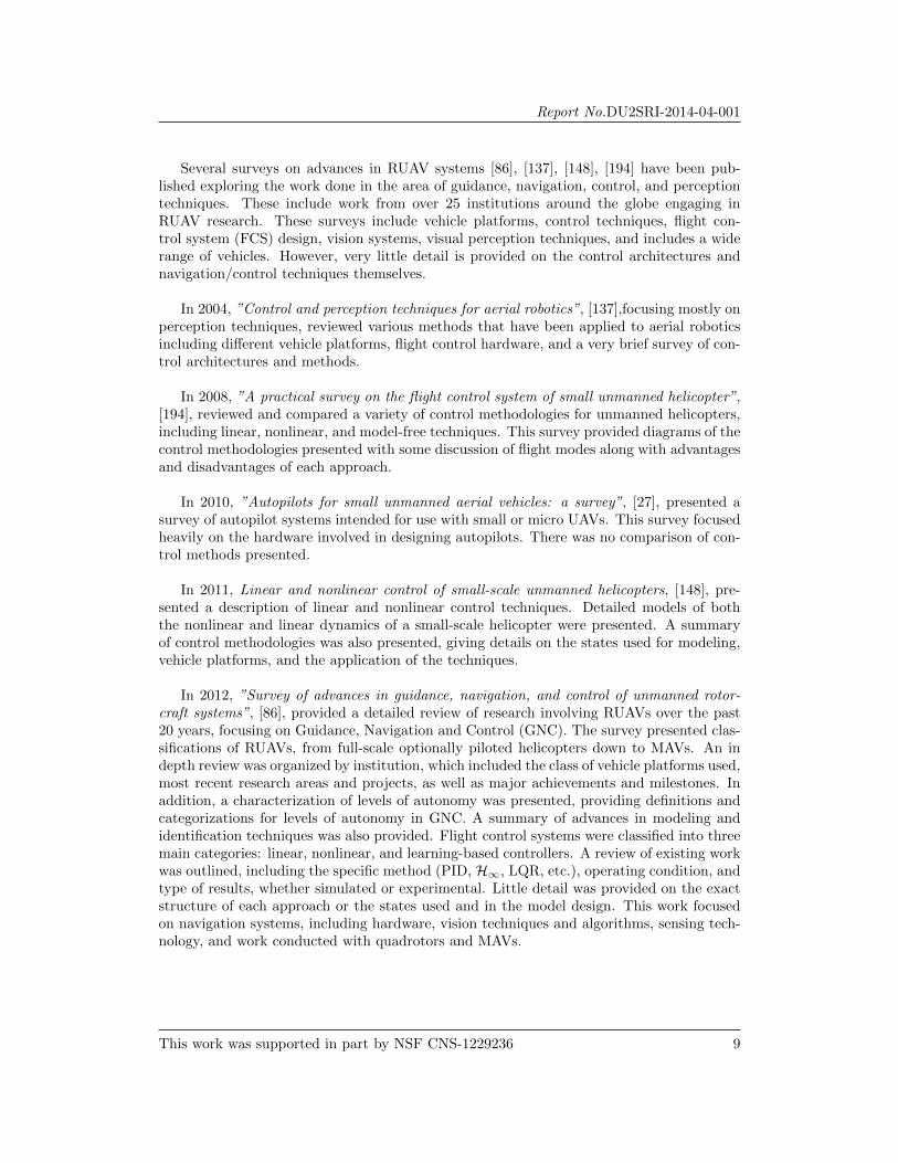
Several surveys on advances in RUAV systems [86], [137], [148], [194] have been pub-lished exploring the work done in the area of guidance, navigation, control, and perceptiontechniques. These include work from over 25 institutions around the globe engaging inRUAV research. These surveys include vehicle platforms, control techniques, flight con-trol system (FCS) design, vision systems, visual perception techniques, and includes a widerange of vehicles. However, very little detail is provided on the control architectures andnavigation/control techniques themselves.

In 2004, ”Control and perception techniques for aerial robotics”, [137],focusing mostly onperception techniques, reviewed various methods that have been applied to aerial roboticsincluding different vehicle platforms, flight control hardware, and a very brief survey of con-trol architectures and methods.

In 2008, ”A practical survey on the flight control system of small unmanned helicopter”,[194], reviewed and compared a variety of control methodologies for unmanned helicopters,including linear, nonlinear, and model-free techniques. This survey provided diagrams of thecontrol methodologies presented with some discussion of flight modes along with advantagesand disadvantages of each approach.

In 2010, ”Autopilots for small unmanned aerial vehicles: a survey”, [27], presented asurvey of autopilot systems intended for use with small or micro UAVs. This survey focusedheavily on the hardware involved in designing autopilots. There was no comparison of con-trol methods presented.

In 2011, Linear and nonlinear control of small-scale unmanned helicopters, [148], pre-sented a description of linear and nonlinear control techniques. Detailed models of boththe nonlinear and linear dynamics of a small-scale helicopter were presented. A summaryof control methodologies was also presented, giving details on the states used for modeling,vehicle platforms, and the application of the techniques.

In 2012, ”Survey of advances in guidance, navigation, and control of unmanned rotor-craft systems”, [86], provided a detailed review of research involving RUAVs over the past20 years, focusing on Guidance, Navigation and Control (GNC). The survey presented clas-sifications of RUAVs, from full-scale optionally piloted helicopters down to MAVs. An indepth review was organized by institution, which included the class of vehicle platforms used,most recent research areas and projects, as well as major achievements and milestones. Inaddition, a characterization of levels of autonomy was presented, providing definitions andcategorizations for levels of autonomy in GNC. A summary of advances in modeling andidentification techniques was also provided. Flight control systems were classified into threemain categories: linear, nonlinear, and learning-based controllers. A review of existing workwas outlined, including the specific method (PID, H∞, LQR, etc.), operating condition, andtype of results, whether simulated or experimental. Little detail was provided on the exactstructure of each approach or the states used and in the model design. This work focusedon navigation systems, including hardware, vision techniques and algorithms, sensing tech-nology, and work conducted with quadrotors and MAVs.



1.1 Scope and Motivation

This research focuses on surveying existing control methods and modeling techniques withthe objective of determining capabilities and effectiveness of algorithms for unmanned au-tonomous flight, navigation, obstacle avoidance, and performance of acrobatics. The sur-veyed control techniques can be fit into one of three categories: linear, nonlinear andmodel-free. After summarizing each controller, and its application, each control approachis categorized accordingly in the comparative table shown in Figure 2. The linear methodsare divided into single-input single-output (SISO) methods and multi-input multi-ouput(MIMO) methods. Proportional-Integral-Derivative (PID) controllers fall under the SISOlinear control category. MIMO linear controllers consist of linear feedback controllers, suchas linear quadratic regulators (LQG) and linear quadratic Gaussian (LQG), H∞ controllers,and gain scheduling controllers that may utilize synthesis techniques. Nonlinear methodsare divided into linearized and fully nonlinear methods. Linearized techniques start with anonlinear model, and utilize various techniques to linearize the system dynamics, includinginput/output feedback linearization. Other methods can then be applied, including adaptivecontrol, model predictive control (MPC), and nested saturation loops. Lastly, backsteppingcontrol approaches utilize fully nonlinear models. Lastly, model free and learning-basedmethods include neural networks (NN), fuzzy logic, and human-based learning techniques.Human-based learning techniques include differential dynamic programming (DDP) and re-inforcement learning.

Figure 2: Control techniques

In order to provide the same reference point for comparison purposes, the followingrationale is used:

• Helicopter model and platform

• Method of identification, including parameter estimation and system modeling



• Control technique and loop architecture

• Flight mode and maneuvers

• Types of results: theoretical, simulated, or experimental



2 Helicopter Dynamics

Rotorcraft have distinct advantages in maneuverability through the use of rotary blades.This design allows rotorcraft to produce the necessary aerodynamic thrust forces withoutthe need of relative velocity. However, control of rotorcraft has inherent complications.These include the complexity of helicopter dynamics due to their heavy nonlinearity andsignificant dynamic coupling between the aerodynamic forces and moments. In addition tononlinearity and dynamic coupling, helicopters are underactuated systems, since there arefewer control inputs than system states.

Figure 3: Basic helicopter configuration showing main and tail rotors.

Helicopter dynamics are generally governed by Six-Degrees-of-Freedom (6-DoF) rigidbody kinematics and dynamics. The forces and moments that affect the vehicle dynamicsare generated by the rotors, body, gravity and aerodynamics. These forces can be eithercontrolled (e.g. rotor thrust) or uncontrolled (e.g. drag forces, wind gusts). The forces aremodeled as functions of the vehicle states, pilot inputs, and environmental factors.

The modeling of aerodynamic forces is complicated and difficult. In order to achieve high-fidelity models of the aerodynamic properties of the vehicle, finite-element techniques areused. This, however, is time consuming and computationally complex. For the purposes ofcontrol design, the system may be divided into lumped-parameter models for each subsystemusing simplified aerodynamics. With this method each subsystem of the helicopter is viewedseparately in order to approximate the dynamics while considering certain assumptions.This approach can significantly reduce the state space of the system and the number ofparameters describing its behavior. The most basic helicopter configuration consists of asingle main rotor and tail rotor, as shown in Figure 3. In addition to the rotors, otherhelicopter components that affect the dynamics are typically lumped into the followingsubsystems for modeling purposes:

i Main rotor

ii Tail rotor

iii Fuselage body

iv Tail horizontal stabilizer (fin)

v Tail vertical stabilizer (fin)

vi Stabilizer or flybar

vii Engine



viii Servo linkages and swashplate

ix Actuators or servos

Figure 4 depicts the typical structure of the helicopter dynamics. The forces and mo-ments generated by each subsystem are determined and, then, combined into generalizedforces and moments relative to a body-fixed coordinate system. These forces, ultimately,drive the helicopter’s rigid body dynamics and kinematics equations, which ultimately de-fine the helicopter dynamic model.

For navigational purposes, a fixed reference coordinate system is established. This isan Earth-fixed coordinate system defined by the designer of the navigational system, andfully dependent on where the vehicle will be operating. Typically, GPS (Global PositioningSystem) receivers are used for navigational feedback.

2.1 Helicopter Rigid Body Equations of Motion

For a 6-DoF rigid body, the motion of the helicopter is defined relative to an inertial ref-erence frame in order for Newtonian mechanics to hold true. An inertial reference framefollows Newton’s first law of motion, where an object is either at rest or moves at a constantvelocity unless acted on by some external force. However, establishing a reference framefixed to the helicopter body significantly simplifies the analysis of forces acting on the he-licopter. In order to derive a set of equations describing the motion of the helicopter twoCartesian reference frames are established.

The first reference frame is chosen fixed to the helicopter body. In a body-fixed Carte-sian frame, FB = OB ,~iB ,~jB ,~kB; the origin is fixed at the helicopter center of mass. Inthis frame, the unit vector ~ib points from the origin outward toward the helicopter nose.The unit vector ~jB points from the origin to the right of the fuselage. The unit vector ~kbpoints downward. The orientation of these vectors in relation to the helicopter body is seenin Figure 5.

The second reference frame is an inertial Earth-fixed Cartesian frame, which follows theNorth-East-Down directional convention. In this Earth-fixed frame, FI = OI ,~iI ,~jI ,~kI.The unit vectors~iI , ~jI , and ~kI , point North, East and down towards the center of the Earth,respectively, as shown in Figure 6.

Rigid body dynamics are governed by the Newton-Euler laws of motion given in (1) and(2). These equations ultimately provide information on translational and angular velocitiesas a result of forces acting on the rigid body.

Fnet =d

dtG(t), (1)

MCMnet =

d

dtHCM (t). (2)

The net external forces, Fnet, are defined as the rate of change of the body’s linearmomentum, G(t). The net external moments about the body’s center of mass, MCM

net , are



Figure 4: Helicopter dynamics.This work was supported in part by NSF CNS-1229236 14


Figure 5: Body-fixed frame coordinate system, [148].

Figure 6: North-East-Down Earth-fixed reference frame, [41].



equal to the rate of change of angular momentum about the center of mass, HCM . Thesemoments are derived here for a rigid body following the procedure in [12].

For a point mass m with linear velocity v, the linear momentum is defined as:

G(t) = m(t)v(t). (3)

The angular momentum of the point mass about a point is defined in (4), where dP isthe distance of the mass from the point.

H(t) = d(t)×m(t)v(t). (4)

For a rigid body, the linear momentum is defined as the sum of infinitesimal linearmomentums of particles that make up an entire body. For each particle, the mass is definedas infinitesimally small, dm, for an infinitesimally small volume dV of density ρ. The totallinear momentum is summed for each particle over the volume of the object:

G =

∫V

vdm, where dm = ρdV. (5)

The total angular momentum of the mass about some point is defined as a sum ofinfinitesimal angular momentums of particles:

H =

∫V

d× vdm. (6)

The position of a particle P relative to the inertial reference frame, pPI is given as:

pPI (t) = pCMI +R(t)dPB (7)

where pCMI is the position of the helicopter center of mass with respect to the inertial frame,R(t) is a rotation matrix between the body-fixed frame and inertial frame, and dPB is thedistance of the particle from the center of mass with respect to the body-fixed frame.

The translational velocity of the particle relative to the inertial reference frame is ob-tained through differentiation of (7) and is given as:

vPI (t) = vCMI (t) + R(t)dPB (8)

where vCMI is the translational velocity of the helicopter center of mass relative to the inertialreference frame. The linear momentum is found by evaluating the integral over the volumeof the body:

GI(t) =

∫V

(vCMI (t) + R(t)dPB)dm = vCMI (t)

∫V

dm+ R(t)

∫dPBdm. (9)

The center of mass of an object is defined as:

dCM =1

m

∫V

dP dm. (10)

Typically, the body-fixed frame origin is defined at the helicopter’s center of mass. Sincethe center of mass from the body-frame origin coincides with the body-fixed frame origin,dCMB = 0. By equating this with (10) and assuming mass is non-zero, then:



∫V

dPBdm = 0. (11)

Additionally, the total mass m is found through integration of the infinitesimal pointmasses over the entire volume of the body and is given as m =

∫Vdm. Using these simpli-

fications the final linear momentum equation becomes:

GI(t) = mvCMI (t). (12)

Next, using (8) the angular momentum about the helicopter’s center of mass with respectto the inertial frame origin is evaluated as:

HCMI (t) =

∫V

dPI (t)× vCMI (t)dm+

∫V

dPI (t)× R(t)dPBdm. (13)

Here, dPI is the distance to the point from the center of mass with respect to the inertialreference frame. This distance may be defined with respect to the body-fixed frame asdPI = R(t)dPB , and is substituted into (13) as:

HCMI (t) =

∫V

R(t)dPB × vCMI (t)dm+

∫V

R(t)dPB × R(t)dPBdm. (14)

In order to further simplify the angular momentum equation, the following propertiesare used. First, the properties of cross products are defined as follows:

a× b = −b× a (15)∫~u× ~vdx = ~u×

∫~vdx = (

∫~udx)× ~v (16)

(Ax)× (Ay) = (detA)A−T (x× y) (17)

where for a 3 × 3 rotation matrix A, det A = 1 and A−T = A. Second, the rigid bodyrotational kinematics, [170], are introduced and given as:

R(t) = R(t)ωB(t) (18)

where ω(t) is the skew-symmetric matrix of the angular velocity vector, ω(t), such that:

x =

0 −x3 x2

x3 0 −x1−x2 x1 0

, for x =

x1

x2

x3

T

, (19)

x× y = xy, (20)

x, y ∈ R3. (21)

These assumptions in (15) – (17), (18), and (19) – (21) and the equality in (11) reduce theangular momentum in (14) to:

HCMI =

∫V

R(t)[dPB × ωB(t)dPB

]dm =

∫V

R(t)dPBωB(t)dPBdm. (22)



By defining dPB = [x y z]T and ωB(t) = [p q r]T it can be shown that dPB×ωB(t)dPB = IωB ,as shown in [12], where I is the inertial tensor of the rigid body. The inertia matrix for therigid body is defined as J =

∫vIdm. The final angular momentum is then given as:

HCI M(t) = R(t)

∫V

IωBdm = R(t)Jωb(t). (23)

The net external moments and forces in terms of the linear moments and angular mo-mentum simplifications described in (12) and (23) are then applied to the Newton-Eulerequations in (1) and (2) to find the forces and moments acting on the body with respect tothe inertial frame and are given as follows:

FI(t) = mvCMI (t), (24)

MCMI = ˙R(t)JωB(t) +R(t)JωB(t). (25)

Finally, the forces and moments can be expressed in the body-fixed frame following theprocedure in [12] as:

FB(t) = m(ωB(t)× vCMB (t) + vCMB

), (26)

MCMB = ωB × JωB(t) + JωB(t). (27)

The helicopter equations of motion described in (26) and (27) are known as the Newton-Euler equations of motion for a rigid body, where fB = FCMB and τB = MCM

B , and aregiven below as: mI3 0

0 J

υB

ωB

+

ωB ×mυB

ωB × JωB

=

fB

τB

. (28)

The forces, moments, and translational velocity may be separated into componentscorresponding to each of the principal axes of the body-fixed frame as fB = [X Y Z]T ,τB = [L M N ]T , and vCMB = [u v w]T , respectively. Transforming the gravity vector fromthe inertial frame, gI = [0 0 g]T , to body-frame results in gB = RT (t)gI , where:

R =

R11 R12 R13

R21 R22 R23

R31 R32 R33

. (29)

The equations of motion with respect to the body-fixed frame are given as:

u = rv − qw +R31g +X/m

v = pw − ru+R32g + Y/m

w = qu− pv +R33g + Z/m

p = qr(Jyy − Jzz)/Jxx + L/Jxx

q = pr(Jzz − Jxx)/Jyy +M/Jyy

r = qp(Jxx − Jyy)/Jzz +N/Jzz

(30)



2.2 Position and Orientation Dynamics

For flight navigation, it is necessary to express the position and orientation of the helicopterwith respect to an Earth-fixed inertial reference frame. To do so, a relationship betweenthe body-fixed and inertial frames must be established in order to provide a method of de-scribing the orientation of the frames relative to one another. This relationship is called therotation matrix R that represents a series of rotations from the body-fixed frame to the finalorientation of the inertial frame, [34, 170]. The rotation matrix is is typically expressedin terms of roll (φ), pitch (θ), and yaw (ψ) Euler angles. These rotations must occur in a

specific sequence, . The first rotation moves the helicopter an angle of φ about the k axis,as seen in Figure 7. The second rotation moves the helicopter an angle of θ about the new jaxis, as seen in Figure 8. Finally, the last rotation moves the helicopter an angle of ψ aboutthe new helicopter i axis, as seen in Figure 9.

Figure 7: Helicopter yaw motion.

Figure 8: Helicopter longitudinal motions. Figure 9: Helicopter lateral motions.

The final rotation matrix is obtained by multiplying the individual rotation matrices in(31) following the properties of transformations in [170]. This final rotation is given as



R = RψRθRφ and is expanded in terms of Euler angles below as:

Rψ =

cosψ sinψ 0

− sinψ cosψ 0

0 0 1

Rθ =

cos θ 0 − sin θ

0 1 0

sin θ 0 cos θ

Rφ =

1 0 0

0 cosφ sinφ

0 − sinφ cosφ

(31)

R(Θ) =

cosψ cos θ cosψ sinφ sin θ − cosφ sinψ sinφ sinψ + cosφ cosψ sin θ

cos θ sinψ cosφ cosψ + sinφ sinψ sin θ cosφ sinψ sin θ − cosψ sinφ

− sin θ cos θ sinφ cosφ cos θ

(32)

In order to determine the orientation dynamics, the time derivative of the rotation matrixis determined and is given in Equation 33. The proof may be seen in [170]:

R = RωB (33)

Next, the time derivative of the rotation matrix in (32), and the relationship in (33),are used to find the orientation dynamics of the helicopter, given in Equations 34 and 35.Details on these derivations can be found in [132, 148, 170, 64]. Here, the Euler angles aredenoted by Θ = [φ θ ψ]T :

Θ =

φ

θ

ψ

= Ψ(Θ)ωB (34)

Ψ(Θ) =

1 sinφ tan θ cosφ tan θ

0 cosφ − sinφ

0 sinφ/ cos θ cosφ/ cos θ

(35)

The position and velocity dynamics together with the orientation dynamics form thecomplete helicopter equations of motion in terms of the helicopter’s body-fixed frame forcesand moments and are given in below as:

pI = vI

vI = 1mRf

B

R = RωB

IωB = −ωB × (IωB) + τB

(36)

Here pI and vI denote the position and linear velocity of the helicopter center of gravity(CG) with respect to an earth-fixed reference frame. The position and orientation trajectorydynamics may be obtained by integrating the rigid body dynamics in (30) along through



the kinematic equations in (36). The inertial position can be found given the body velocitiesthrough pI = vI = RvB . The euler rates can be found through the relationship Θ = Ω(Θ)ωbin (34):

xI = cθcψu+ (sθsφcψ − cφsψ)v + (sθcφcψ + sφsψ)w (37)

yI = cθcψu+ (cφcψ + sφsψsθ)v + (cθsψsθ − cψsφ)w (38)

zI = −sθu+ cθsφv + cφcθx (39)

φ = p+ sφtθq + cφtθr (40)

θ = cφq − sφr (41)

ψ =sφcθq +

cφcθr (42)

2.3 Forces and Torques

A result of the main and tail rotor rotation is the generation of thrust and torques actingon the helicopter body. Gravity is also acting on the body of the helicopter, and must betaken into account while determining the total body forces on the helicopter. The forcesand torques acting on the helicopter are functions of the main rotor thrust, TMR, tail rotorthrust, TTR, and the main rotor cyclic angles, a1 and b1, [64].

2.3.1 Main Rotor Forces

The thrust generated by the main rotor results in a translational force on the helicopter.This thrust is perpendicular to the Tip-Path-Plane (TPP), Figure 10, which is the planeformed by the blade tips. This force vector can be decomposed into components along thebody-frame x, y, and z axis. The magnitude of the thrust vector is represented as TMR. Thecomponents of the main rotor forces as a result of the blade flapping and thrust are given as:

FBMR =

XMR

YMR

ZMR

=

−TMRsin(a1)

−TMRsin(b1)

−TMRcos(a1)cos(b1)

(43)

2.3.2 Tail Rotor Forces

Unlike the main rotor, the tail rotor generates a force perpendicular to the rotor hub. Thepilot has no control of the flapping angles. As a result, the resulting force component is inthe y-direction only. The components of the tail rotor thrust are given in (44):

FBTR =

XTR

YTR

ZTR

=

0

TTR

0

(44)



2.3.3 Gravity

The gravitational force on the helicopter is represented in the inertial Earth-fixed frame inthe downward direction. Thus, the gravity vector is given as F Ig = [0 0 mg]T . This forcemay be expressed as components with respect to the body-fixed frame as given in (45),[12, 64, 102].

FBg =

Xg

Yg

Zg

= R(Θ)F Ig =

−sin(θ)mg

sin(φ)cos(θ)mg

cos(φ)cos(θ)m]cdotg

(45)

2.3.4 Torques

The torques acting on the body of the helicopter are a result of the forces being offset fromthe center of gravity. The relation below defines the relationship between the force (F ),distance (d) and the resultant torque:

τ = Fd (46)

2.3.5 Main Rotor Torque

For the main rotor torque, the distance offset of the main rotor from the helicopter centerof gravity is defined as [lm, ym, hm]T , [147]. The resulting torque contributed by the mainrotor is given as:

LMR

MMR

NMR

=

YMRhm − ZMRym

−XMRhm − ZMRlm

XMRym + YMRlm

(47)

2.3.6 Tail Rotor Torque

For the tail rotor torque, the distance offset of the tail rotor from the helicopter center ofgravity is defined as [lt, 0, ht]

T . The resulting torque contributed by the main rotor is givenby:

LTR

MTR

NTR

=

YTRht

0

−YTRlt

(48)



2.3.7 Main Rotor Drag

The main rotor generates an aerodynamic drag as it rotates. This drag results in a torque,QMR, [64, 93]. This torque is perpendicular to the TPP and it can be decomposed intocomponents along the body frame by projecting the torque vector on to the hub plane. Theresultant components are given as:

LD

MD

ND

=

QMRsin(a1)

−QMRsin(b1)

QMRcos(a1)cos(b1)

(49)

2.4 Rotor

The helicopter receives most of its propulsive force from the main and tail rotors. Theaerodynamics of the rotors, especially that of the main rotor, are highly nonlinear andcomplex. In order to reduce the complexity and simplify the dynamics for use in modelingand control design, a number of assumptions are considered, [12, 148, 29, 147] as follows:

• Rotor blades are rigid in both bending and torsion

• Small flapping angles

• Uniform inflow across rotor blade, no inflow dynamics used

• Effects of coning, due to flapping angles, is constant

• Forward velocity effect omitted

• Coupling ratio for pitch-flap is disregarded

• Constant rotor speed

The dynamics of the main and tail rotors are controlled by input control commands.However, they are also affected by the motion of the helicopter. These control commandsare represented by ~uc = [δlon δlat δped δcol]

T . The thrust magnitudes of the main and tailrotors are controlled by the collective commands δcol and δped, respectively. The main rotorblade flapping dynamics is controlled by the cyclic inputs δlon and δlat, which control thetilt of the TPP. Control of the propulsive forces is achieved by controlling the direction andinclination of the TPP. Thrust produced by the rotor blades is perpendicular to the TPP.

The orientation of the TPP is dependent on main rotor blade flapping dynamics. Duringrotation, the blades exhibit a flapping motion, Figure 11, a lead-lagging motion, Figure 12and a pitching motion of the blade, Figure 13. These motions make-up the rotor blade DoFand are denoted by β, ξ, and ζ, respectively.

2.4.1 Lift and Drag

The aerodynamic forces on the rotor blade depend on the 3-DoF orientation of the bladeat any time. The blade’s pitch angle, ζ, affects the lift and drag of the blade elements.The flapping angle of the blade affects the inertial forces on the blade along the direction



Figure 10: Helicopter Tip-Path-Plane (TPP).

Figure 11: Helicopter blade flapping motion.

Figure 12: Helicopter blade lead-lagging motion.



Figure 13: Helicopter blade pitching motion.

of the main rotor thrust vector. In determining the lift and drag generated by the mainrotor requires consideration of the blade’s flapping motion, ζ, helicopter forward velocitywith respect to the air, also known as free stream velocity and denoted by V∞, rotation ofthe blade about the shaft in the form of angular velocity, Ω, and also the inflow velocity ofair through the rotor, [148]. This total air velocity on the blade, U , can be decomposed intothree components. These components are defined in relation to the plane perpendicularto the rotor shaft, known as the hub plane. The plane hub frame is defined as Fh =Oh, ~ih, ~jh, ~kh; where ~ih points backwards towards the tail, ~jh points to the right of thehelicopter, and ~kh points up. Two components are in the hub plane while the third is out ofthe plane. All three components are normal to the hub plane. The out of plane component isperpendicular to the hub plane pointing downward and is denoted by UP , as seen in Figure14(c). The next component, UT , is parallel to the hub plane and tangential to the bladein the direction of the blade rotational motion as seen in Figure 14(a) and (d). The lastcomponent, UR, lies on the hub plane and points radially pointing outward in the directionof and parallel to the blade, as seen in Figure 14(a) and (c). The total air velocity seen bythe blade is given as:

U =√U2T + U2

P . (50)

At any time during flight, the blade experiences a pitch angle, ζ, related to the angle ofattack αb of the blade with respect to the airstream U , which approaches the blade at aninflow angle φb. This relationship is given by (51), as seen in Figure 15:

ζ = αb + φb. (51)

The UT component is defined in terms of the blade angular velocity and the componentof the free stream velocity in the direction parallel to the hub plane as:

UT = Ωr + V∞cosαhbsinψb. (52)

The UP component is defined in terms of the main rotor flapping, the blade angular velocity,



(a) Rotor top view. (b) V∞ and vi relative to hub plane.

(c) Rotor side view. (d) 2D blade element.

Figure 14: Air velocity components relative to the blade element. [148]



the free stream velocity component perpenticular to the blade, and the inflow velocity ui,and is given as:

UP = rβ + (V∞cosαhbsinψb + Ωr)sinβ + V∞sinαhbcosβ + uicosβ (53)

= rβ + V∞cosαhbsinψbβ + Ωrβ + V∞sinαhb + ui. (54)

It should be noted that here r represents the distance from the rotor shaft along the blade.It is not to be mistaken for the pitch angular rate.

Figure 15: Helicopter blade cross-section. [148]

The lift and drag on the blade are determined through blade element analysis. Byconsidering the blade as a two-dimensional airfoil, the lift and drag vectors at each bladeelement may be determined. The infinitesimal lift of the blade element dr is given as:

dL = 1/2ρaU2cbClααbdr. (55)

The infinitesimal drag of the blade element is given as:

dD = 1/2ρaU2cbCddr. (56)

Here, ρa is the air density, cb is the blade chord, Clα is the blade lift coefficient, CD is theblade drag coefficient, and αb is the blade angle of attack with respect to the air velocity U .The total lift and drag may then be derived by integrating along the distance of the blade,r, from the rotor to the end of the blade length, Rb.

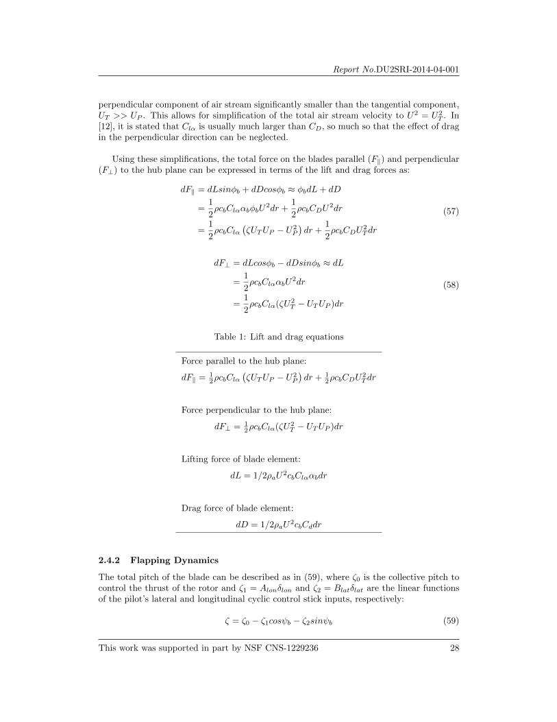
The forces perpendicular and parallel to the hub plane can be expressed in terms of thelifting and drag forces. These are given in (57) and (58). Since it is assumed that the inflow

angle is very small, sinφb ≈ φb, cosφb ≈ 1 − φ2

2 ≈ 1, and tan ≈ φb. Then, the relationship

between the inflow angle and the air stream velocity components, tanφb = UPUT

, becomes

φb = UPUT

. The angle of attack can then be written as αb = ζ − UPUT

= ζUT−UPUT

. In additionto the small inflow angle, the rotor rotational speed is assumed to be high, making the



perpendicular component of air stream significantly smaller than the tangential component,UT >> UP . This allows for simplification of the total air stream velocity to U2 = U2

T . In[12], it is stated that Clα is usually much larger than CD, so much so that the effect of dragin the perpendicular direction can be neglected.

Using these simplifications, the total force on the blades parallel (F‖) and perpendicular(F⊥) to the hub plane can be expressed in terms of the lift and drag forces as:

dF‖ = dLsinφb + dDcosφb ≈ φbdL+ dD

=1

2ρcbClααbφbU

2dr +1

2ρcbCDU

2dr

=1

2ρcbClα

(ζUTUP − U2

P

)dr +

1

2ρcbCDU

2T dr

(57)

dF⊥ = dLcosφb − dDsinφb ≈ dL

=1

2ρcbClααbU

2dr

=1

2ρcbClα(ζU2

T − UTUP )dr

(58)

Table 1: Lift and drag equations

Force parallel to the hub plane:

dF‖ = 12ρcbClα

(ζUTUP − U2

P

)dr + 1

2ρcbCDU2T dr

Force perpendicular to the hub plane:

dF⊥ = 12ρcbClα(ζU2

T − UTUP )dr

Lifting force of blade element:

dL = 1/2ρaU2cbClααbdr

Drag force of blade element:

dD = 1/2ρaU2cbCddr

2.4.2 Flapping Dynamics

The total pitch of the blade can be described as in (59), where ζ0 is the collective pitch tocontrol the thrust of the rotor and ζ1 = Alonδlon and ζ2 = Blatδlat are the linear functionsof the pilot’s lateral and longitudinal cyclic control stick inputs, respectively:

ζ = ζ0 − ζ1cosψb − ζ2sinψb (59)



As seen in Figure 16, the blade is modeled as a rigid thin plate rotating about the shaftat an anglar rate of Ω. The angular position of the blade in the hub plane is denoted asψb measured from the tail axis. The blade flapping hinge is modeled as a torsional springwith stiffness Kβ . The moments acting on the blade are due to the lifting force describedin Section 2.4.1, weight of the blade (MW ), the inertial forces acting on the blade (Mi andMc), and the restoring force of the spring (MKβ ). Equating all the moments acting on theblade results in (66). Substituting (61) – (65) into (66) results in (67), where the blade’sinertia is given by:

Ib =

∫ Rb

0

mbr2dr (60)

Figure 16: Blade spring model, [148].

MW =

∫ Rb

0

mbgrcosβdr =1

2mbgR

2b (61)

MKβ = −Kββ (62)

ML =

∫ Rb

0

rdFadr =1

2ρcbClα

∫ RB

0

r(ζU2T − UTUP )dr (63)

Mc =

∫ Rb

0

rdFcsinβ =

∫ Rb

0

mbΩ2r2cosβsinβdr = Ω2βIb (64)

Mi =

∫ Rb

0

rdF i =

∫ Rb

0

mbβr2dr = βIb (65)

Mi +Mc +MKβ +MW = ML (66)

β + (Ω2 +Kβ

Ib+

1

2IbmbgR

2b)β =

1

2IbρcbClα

∫ RB

0

r(ζU2T − UTUP )dr (67)

The flapping dynamics, β(t) in (68), can be expressed as a Fourier series neglecting thehigher order terms, only keeping the first order harmonics:



β(t) = a0 − a1cosψb − b1sinψb (68)

Substituting (68), its first and second time derivatives, (54), and (52) into (67), theequations can then be written as a system of the form x + Dx + Kx = F . Here, the statevector x = [a0 a1 b1]T , the coning, longitudinal tilt, and lateral title angle of the TPP. Thestate space representation is given below in (69), where x1 = x and x2 = x: x1

x2

=

0 I

−K −D

x1

x2

(69)

The TPP dynamics are simplified, [12, 148], by assuming a constant coning angle, dis-regarding the hinge offset, assuming a zero pitch-flap coupling ratio, and disregarding theeffects of forward velocity. The simplified dynamics are given in (70) for the longitudinaldynamics and (71) for the lateral dynamics.

τf a = −a− τfq +Abb+Alonδlon (70)

τf b = −b− τfp+Bba+Blatδlat (71)

Here, the time rotor constant, τf , is a function of the angular velocity, Ω, and the Locknumber, γ.

τf =16

γΩ(72)

γ =ρaClαR

4b

Ib(73)

Additionally, Ab and Ba are the rotor cross coupling terms:

Ab = −Ba =8

γ(λ2b − 1) (74)

and λβ is the flapping frequency ratio:

λ2β =Kβ

Ω2Ib+ 1. (75)

2.4.3 Main Rotor Forces

The total thrust and counter-torque produced by the main rotor is a function of the forcesacting on the blades perpendicular and parallel to the hub plane. The expressions are givenas:

Tmr =Nmb2π

∫ 2π

0

∫ Rt

0

dF⊥,tcosβdψm (76)

Qmr =Nmb2π

∫ 2π

0

∫ Rt

0

ldF‖,tdψm (77)

From here, the individual body-fixed frame components may be determined followingthe equations in section 2.3.



2.4.4 Tail Rotor

Unlike the main rotor, the tail rotor only has a collective pitch, ζt. The tail rotor bladeexperiences induced air velocity and has flow components similar to (54) and (52), but withcoefficients and constants specific to the tail rotor. Additionally, the perpendicular andparallel force components resemble (57) and (58) of the main rotor. The tail rotor thrustand counter-torque can be found using (78) and (79), [12].

Ttr =Ntb2π

∫ 2π

0

∫ Rt

0

dF⊥,tdψt (78)

Qtr =Ntb2π

∫ 2π

0

∫ Rt

0

rdF‖,tdψt (79)



3 Linearization

3.1 Trim

Aircraft in steady flight must operate at some conditions where the forces and moments arein equilibrium about the center of gravity. This is when the helicopter is in what is known astrim flight, [147]. Trim conditions correspond to certain trim values of the state and inputvariables, given by x0 and δi, respectively. The first step in determining trim values for thehelicopter, is to define the equations of equilibrium and reference flight conditions. Thesetrim values can be found both analytically, as seen in [147], or numerically, as seen in [152].

Figure 17: Forces and moments on the helicopter in trim flight, [147].



3.2 Linearization

There are two main methods to perform linearization of nonlinear dynamic equations. Thefirst is to use Taylor series expansion about some initial condition, [64]. The second methodis to follow small perturbation theory. Small perturbation theory is widely used to linearizethe nonlinear helicopter dynamics about a trim flight condition, usually hover. Examples ofthis are seen in [39, 147, 148, 152]. In the case of the helicopter dynamics, the total force ismade up of the forces and torques contributed by the various helicopter subsystems. Theseforces are either controlled, as a result of the pilot input, or uncontrolled, as a result of thedynamic parameters. These various forces are listed in Table 2.

Table 2: Input force categorized as controlled versus uncontrolled.

Force Type Notation Description

Controlled fδcol Collective input

fδped Tail rotor collective

fδlat Lateral cyclic

fδlon Longitudinal cyclic

fδthr Throttle

Uncontrolled fu, fv, fw Translational velocities

fp, fq, fr Angular rates

fφ, fθ, fψ Orientation angles

fa1 , fb1 Main rotor cyclic angles

fc1 , fd1 Stabilizer cyclic angles

Small perturbation analysis involves applying a small incremental force, ∆f , resultingin small perturbations to the dynamics. For the helicopter, the dynamic parameters thatmake up the state vector are given in (80), while the dynamic inputs are given by (81).

In most cases, the engine throttle is not controlled by the pilot, but rather remainsconstant during flight. As a result, the engine throttle is not included in the input vector.

~x = [u v w p q r φ θ ψ a1 b1 c1 d1 ]T

(80)

~uc = [δcol δped δlat δlon]T

(81)

In [39], the forces and moments are defined to be strictly functions of the state andinput variables. This allows for the forces and moments to be defined as linear functionsof the disturbed variables, ∆xi and ∆δi. This combination is seen in (83). Although itmay be desired to retain terms of higher order derivatives or nonlinear terms for the sake ofaccuracy and completeness, as in [102], many times only the first order terms are considered.



It is noted that for small enough motion, the effects of the nonlinear terms (e.g., ∂2F∂x2 ), and

derivatives of dynamic parameters, (e.g., u, q), are insignificant, [138]:

Fx =∂f

∂x|x0 =

f(x+ ∆x)− f(x)

∆x(82)

∆F =∑xi∈~x

Fxi ·∆xi +∑δi∈~u

Fδi ·∆δi (83)

The derivatives with respect to the controlled inputs are referred to as the control deriva-tives, while those with respect to the uncontrolled states are known as the stability deriva-tives. The notation is simplified to ∂f

∂α = Fα. The derivatives are listed in Table 3.

Table 3: Control and stability derivatives.

Derivative Type Notation Description

Control Derivatives Fδcol Collective input

Fδped Tail rotor collective

Fδlat Lateral cyclic

Fδlon Longitudinal cyclic

Fδthr Throttle

Stability Derivatives Fu, Fv, Fw Translational velocities

Fp, Fq, Fr Angular rates

Fφ, Fθ, Fψ Orientation angles

Fa1 , Fb1 Main rotor cyclic angles

Fc1 , Fd1 Stabilizer cyclic angles

The forces and moments of the helicopter dynamics, which drive the rigid body dynamicsin (30), are shown in Table 4. A small increment of each of these forces and moments isa sum of the derivatives and perturbations, as given in Table 3 and (83), and are given in(84).

∆X = Xu∆u+Xv∆v + · · ·+Xδcol∆δcol + · · ·∆Y = Yu∆u+ Yv∆v + · · ·+ Yδcol∆δcol + · · ·∆Z = Zu∆u+ Zv∆v + · · ·+ Zδcol∆δcol + · · ·∆L = Lu∆u+ Lv∆v + · · ·+ Lδcol∆δcol + · · ·∆M = Mu∆u+Mv∆v + · · ·+Mδcol∆δcol + · · ·∆N = Nu∆u+Nv∆v + · · ·+Nδcol∆δcol + · · ·

(84)

Next, small perturbations are applied to the rigid body dynamics given in (30). It isassumed that the perturbations and any derivative have very small values. As a result,



Table 4: Force and moment components.

Force X X component force

Y Y component force

Z Z component force

Moment L Moment about the X-axis

M Moment about the Y-axis

N Moment about the Z-axis

the product of perturbations are subsequently very small, and negligible, [148]. Theseassumptions result in the following properties, shown in (86). Applying the perturbedvariable in Table 5 to the the forward velocity component of the rigid body dynamics in(30) produces to (85).

u0 + ∆u = (r0 + ∆r)(v0 + ∆v)− (q0 + ∆q)(w0 + ∆w)− sin(θ0 + ∆θ)g +X0 + ∆X

m(85)

The perturbed dynamic equation for forward velocity can be further simplified by usingthe properties in (86).

∆x∆y = 0

cos(∆θ) = 1

sin(∆θ) = ∆θ

sin(θ0 + ∆θ) = sin θ0 + ∆θ cos θ0

sin(θ0 + ∆θ) = sin θ0 + ∆θ cos θ0

(86)

0 = −sinθ0g +X0/m (87)

Table 5: Perturbed Variables

u = ∆u+ u0 p = ∆p+ p0 φ = ∆φ+ φ0

v = ∆v + v0 q = ∆q + q0 θ = ∆θ + θ0

w = ∆w + w0 r = ∆r + r0 ψ = ∆ψ + ψ0

Following this same procedure, and applying the perturbed variables in Table 5 to theentire set of dynamic equations (30) and (37) – (42), along with the flapping dynamics (70)– (71) and the tail stabilizing gyro dynamics as given in [124]. The derived set of lineardynamic equations is given in Tables 6, 7, and 8. This set of dynamic equations is derived



following procedures from [147, 138, 124, 148, 39]. The dynamics may further be simplifiedaccording to the assumed flight condition (i.e., hover, cruise, turn, etc.).

At trim, it is assumed that the helicopter is operating in hover conditions where, u0 =v0 = w0 = p0 = q0 = r0 = 0. Additionally, it is assumed that there are no disturbances sothat δu = δu = δθ = δX = u0 = 0. Given these assumptions, the forward velocity dynamicsin (85) becomes (87). The set of equilibrium equations are derived and given as:

X0 = mgsinθ0 (88)

Y0 = −mgsinφ0cosθ0 (89)

Z0 = −mgcosθ0cosφ0 (90)

L0 = M0 = N0 = 0 (91)

xI = u0cosθ0 (92)

yI = 0 (93)

zI = −u0sinθ0. (94)

At level cruise, the trim conditions mimic those of hover except that the intial conditionfor translational velocity, usually forward, is set to a non-zero value. In the case of levelforward flight, u0 = u0 6= 0. In [134], the trim condition for a level banked turn is givenusing a constant forward velocity, constant yaw angle, and no sideslip.


Repo

rtN

o.D

U2S

RI-2014-04-001

Table 6: State Vector ~x

x =[u v w p q r φ θ ψ a1 b1 c1 d1 rfb

]T

Table 7: State Space A Matrix

Xu Xv + r0 Xw − q0 Xp Xq − w0 Xr + v0 0 −gcθ0 0 Xa1 0 0 0 0

Yu − r0 Yv Yw + p0 Yp + w0 Yq Yr − u0 gcφ0cθ0 −gsφ0sθ0 0 0 Yb1 0 0 0

Zu + q0 Zv − p0 Zw Zp − v0 Zq + u0 Zr −gsφ0cθ0 −gcφ0sθ0 0 Za1 Zb1 0 0 0

Lu Lv Lw Lp Lq + Jpr0 Lr + Jpq0 0 0 0 0 Lb1 0 0 0

Mu Mv Mw Mp + Jqr0 Mq Mr + Jqp0 0 0 0 Ma1 0 0 0 0

Nu Nv Nw Np + Jrq0 Nq + Jrp0 Nr 0 0 0 0 0 0 0 Nrfb

0 0 0 1 sφ0tθ0 cφ0tθ0 0 Ω/cθ0 0 0 0 0 0 0

0 0 0 0 cθ0 −sθ0 −Ωcθ0 0 0 0 0 0 0 0

0 0 0 0 sφ0/cθ0 cφ0

/cθ0 (q0sφ0− r0cφ0

)tθ0/cθ0 (q0cφ0− r0sφ0

)/cθ0 0 0 0 0 0 0

0 0 0 0 −1 0 0 0 0 −1/τf Ab Ac 0 0

0 0 0 −1 0 0 0 0 0 Ba −1/τf 0 Bd 0

0 0 0 0 −1 0 0 0 0 0 0 −1/τs 0 0

0 0 0 −1 0 0 0 0 0 0 0 0 −1/τs 0

0 0 0 0 0 Kr 0 0 0 0 0 0 0 Krf b

Th

isw

ork

was

supp

ortedin

part

by

NS

FC

NS

-122923637

Repo

rtN

o.D

U2S

RI-2014-04-001

Table 8: State Space B Matrix

B :

Xδlat Yδlat Zδlat Lδlat Mδlat Nδlat 0 0 0 Alat Blat 0 Dlat 0

Xδlon Yδlon Zδlon Lδlon Mδlon Nδlon 0 0 0 Alon Blon Clon 0 0

Xδped Yδped Zδped Lδped Mδped Nδped 0 0 0 0 0 0 0 0

Xδcol Yδcol Zδcol Lδcol Mδcol Nδcol 0 0 0 0 0 0 0 0

T

Th

isw

ork

was

supp

ortedin

part

by

NS

FC

NS

-122923638


4 Control Approaches

Considerable research has already been conducted in the area of flight control for rotorcraft.The platforms used in design of flight control systems and navigational control algorithmsrange from full to small scale rotorcraft which can be flown with or without pilot commandsand, especially in early research, may have been mounted on an experimental gimbaledstand for ease of indoor flight. Advances in both sensing and computing technology has ledto increased precision and reliability as well as significantly higher update rates in necessarynavigational sensors (i.e. GPS, IMUs, etc.) as well as increased processing capabilities forthe flight computer. As a result, along with advancements in control theory, a number ofcontrol strategies have been implemented for various flight modes and maneuvers of therotorcraft, validated using numerical simulations and/or experimental results.

Flight controllers typically fit in one of three main categories - linear, nonlinear, ormodel-free - depending on the model representation used to describe the dynamics of therotorcraft. The dynamics of the rotorcraft are inherently nonlinear, making determinationof a full and accurate model difficult. The rotorcraft is an underactuated system, since thereare significantly fewer control inputs than states to be controlled. There is major dynamiccoupling between the control inputs and the states, that is, each input affects multiple statesand may cause unintended responses. Nonlinear models are the most difficult to identifyand implement due to the complexity of the equations and often high order of polynomialor differential equation necessary to fully describe the system dynamics. Additionally, thereare a number of phenomena that exist in nonlinear systems, such as the existence of mul-tiple equilibria and modes of behavior that cannot be described by a linear model. Linearcontrollers use a number of assumptions in order to simplify the nonlinear dynamic models.Usually, this linearization occurs about some particular condition. They also are usuallyonly valid in a small subset of the entire flight envelope. This limits the capability, maneu-vers and flight scenarios of linear controllers. Despite their drawbacks, linear controllers arestill the easiest to design and implement. Finally, model-free control designs, as the namesuggests, do not require a model of the helicopter dynamics. Instead, model-free controldesigns utilize learning or human based algorithms. These types of controllers tend to relyheavily on pilot commanded flight testing in order to teach the algorithms to mimic thehuman pilot behavior and decision making.

Regardless of the type of flight controller used, the control architectures consist of anumber of interconnected loops in order to control navigation, translational dynamics andattitude dynamics of the helicopter. For rotorcraft, the attitude dynamics are much fasterthan the translational dynamics. Typically, flight controllers are designed with at least twoloops. The inner most loop controls the attitude dynamics. The next outer loop dealswith translational dynamics. An additional outer-most loop may be used for navigationalguidance, such as trajectory generation or tracking. A second approach to the control archi-tecture is to separate the lateral-longitudinal dynamics from the heave-yaw dynamics. Bothapproaches associate the system inputs with a rigid-body dynamic state to be controlled.These states include translational positions and velocities, angular rates, and attitude an-gles. However, since rotorcraft are underactuated systems, there are more states than inputsto the helicopter dynamics. In order to deal with this, many of the helicopter states may beused as intermediate or virtual inputs to subsequent cascaded loops. Generally, the rotor-craft main rotor collective and throttle are associated with heave, or altitude. The tail rotor



collective is associated with the yaw motion. Lastly, the main rotor lateral and longitudinalcollectives are associated with the roll and pitch of the helicopter which subsequently resultin lateral and longitudinal translation. A third, less frequently used, approach uses classicalcontrol analysis in order to manipulate system poles and gain or phase margins to stabilizethe helicopter. However, even this structure utilizes multiple loops.

4.1 Control Architecture Structures

Depending on the type of flight maneuver desired to achieve, the design of the control looparchitecture varies. This is due to the assumptions or simplifications that can be madeand the type of reference input to follow. The most common types of flight controllers canbe separated into the following categories: yaw or heading control, attitude or orientationcontrol, altitude control, velocity control, position control. Each of the control structurescan be designed using simplified dynamic models specific to the navigational dynamic statesand particular flight mode to be controlled. These same controllers may be combined inorder to achieve more advanced maneuvers, such as hover control and trajectory tracking.

4.1.1 Hover Control

Hover control is the most basic of maneuvers. Most linearizations of dynamic models aredone assuming hover conditions. At hover, the goal is to keep the helicopter at a desiredposition, sometimes while maintaining a certain heading or yaw rate.

4.1.2 Yaw or Heading Control

The rotorcraft yaw rate or heading can be controlled using the tail rotor collective input.One important consideration for control of yaw is the possible presence of a yaw-rate gyroin RC helicopters. These gyros are used to provide stabilization in the yaw channel duringpiloted flight and have their own dynamics that are not described by the dynamic equationsof the helicopter. It is possible to create model of the gyro dynamics through comparisonof flight tests with and without the gyro. This is done in [140, 124]. The yaw dynamicsare most easily decoupled for a helicopter in hover, while in translational flight a changein heading will affect the lateral-longitudinal dynamics. However, for very small changesin heading or at low enough velocities, the controller can be successful. A basic structureof a yaw controller, shown in Figure 18, may take in as a reference command a constantyaw angle or a yaw rate depending on the maneuver to be performed. The control blockrepresents any time of control that might be used, typically a PID controller.

Figure 18: Yaw control block diagram.



4.1.3 Attitude or Orientation Control

Attitude control is used to stabilize the orientation of the rotorcraft. A typical attitudecontrol architecture is shown in Figure 19. This control structure uses the rotorcraft cyclicinputs for pitch and roll and tail rotor collective for yaw stabilization. Attitude control isplaced as an inner loop. Typically, an attitude controller will either regulate the pitch androll only, the yaw only, or all three. This can depend on how the controller will be used inthe FCS, whether as part of a larger control structure, such as one for hover or trajectorytracking. For a SISO control architecture, a single controller is used for each channel. How-ever, with MIMO approaches, such as LQR and H∞, a single controller may be responsiblefor two or more channels at once. The method of decoupling the dynamics will determinehow these channels can be lumped. However, most approaches keep the pitch and roll anglestogether.

Figure 19: Attitude/orientation control block diagram.

4.1.4 Velocity Control

Velocity control is used to ensure that a particular velocity trajectory is achieved. Usually,this is used for cruise flight in parallel with a heading and attitude controller or in a trajec-tory tracking scheme in order to generate virtual attitude commands for the inner loop ofthe FCS, given desired positions or velocities. A typical architecture for velocity control isgiven in Figure 20. For SISO schemes, the control blocks represent individual controllers foreach channel. However, a MIMO control approach can be used. In most cases, the lateraland longitudinal translational velocities u and v are controlled together. The velocity con-trol block will generate desired roll and pitch orientation angles or rates in order to achievethe desired velocity and feed that virtual command to the inner loop attitude controller.

4.1.5 Altitude Control

Altitude control is used to ensure the helicopter maintains a desired height during flight.The main rotor collective and, if controllable, the engine throttle inputs are regulated inorder to maintain the desired altitude. Sometimes, altitude control is coupled with the inner



Figure 20: Velocity control block diagram.

loop attitude control and decoupled from the lateral-longitudinal dynamics. This is knownas lateral-longitudinal outerloop and heave-yaw inner-loop control. In this type of structure,the outer-loop controller produces the reference roll and pitch trajectories for the inner-loopcontroller. One such example is given below in Figure 21.

Figure 21: Lateral-longitudinal and heave-yaw control structure.

Another approach uses two individual controller to handle decoupled longitudinal-verticaland lateral-directional dynamics. This type of structure is shown below in Figure 22.

4.1.6 Position Control and Trajectory Tracking

Position control and trajectory tracking is achieved by providing a desired trajectory refer-ence to the FCS. In order to achieve this, a combination of velocity, altitude, and orientationcontrol must be used. This is shown in Figure 23. For position control, it may be desired



Figure 22: Longitudinal-vertical and lateral-directional control structure.

to maintain the helicopter at a particular position. This can be achieved by a two loopstructure. The outermost loop takes the desired position and determined the necessaryhelicopter orientation in order to maintain that position. The innermost loop will then de-termine necessary helicopter control inputs. A three loop structure may also be used. Herethe outer-most loop uses the desired trajectory in order to determine desired translationalvelocities. These velocities act as virtual inputs to the middle loop, which determines idealattitude trajectories as inputs the the inner-most loop. This inner-most loop determinedthe necessary helicopter control inputs. Trajectory tracking may have the additional re-quirement of maintaining a desired heading trajectory.

Figure 23: Block diagram for trajectory tracking.

4.2 Control Methods

In this section, two main classifications of control methods used in rotorcraft navigation andcontrol are presented. For each classification, specific methods are presented, giving detailson the theory and how they are used in the overall control architecture. For linear methods,PID, LQR/LQG,H∞, and gain scheduling techniques are presented. For nonlinear methods,backstepping, adaptive, model predictive, linearization, and nested saturation techniquesare presented. Table 9 summarizes the advantages and disadvantages of each approach and



lists typical maneuvers that have been achieved, either in simulation or experimentally, byvarious groups. Lastly, a comprehensive overview of the control approaches is given in Table10.



Table 9: Comparison of Control Methods

Control Algorithm Advantages Disadvantages Maneuvers

LIN

EAR

PID (SISO)

Easily implemented

Assumes simplified de-coupled dynamics

Gains can be tuned inflight

Lacks robustness

Ignores coupling of dy-namics

Mostly hovered flight

Attitude/Altitudecontrol

Lateral/ Longitudinalcontrol

LQG/ LQR

Multivariable capabil-ities

Used to stabilize bothinner and outer loops

-

Limited to certainflight conditions

Gain calculation is aniterative process

-

Hovering

Trajectory tracking

-

H∞

Deals with parametricuncertainty

Can handle unmod-eled dynamics can beused for loop-shaping

High level of math un-derstanding and com-putation

Need a reasonablygood system model

Hovering

Trajectory tracking

-

GainScheduling

Larger range of flightenvelope and operat-ing conditions

Can use a bank of sim-ple controllers

Requires ability tostore a number ofgains and controlapproaches

Transition betweenswitches might beunsteady

Hovering

Trajectory tracking

NONLIN

EAR Back-stepping

Good techniquefor underactuatedsystems

Need a nonlinearmodel

Trajectory tracking

FeedbackLinearization

Can deal with nonlin-earties while allowingfor application of lin-ear techniques

-

Higher computationalcomplexity

Transformed variablesand actual output mayvary greatly

Auto take-off andlanding

Hovering and aggres-sive maneuvers

AdaptiveControl

Robust technique

Can adapt to unmod-eled dynamics andparametric uncer-tainty

Complex analysis

Need good knowledgeof the system

Formation flight

Vision based naviga-tion

ModelPredictiveControl(MPC)

Can predict future be-havior, to some extent

Can place constraintson the input

Tracking errors can beminimized

Prediction modelmust be formulatedcorrectly

-

-

Target tracking

-

-



4.2.1 Linear PID Controllers

PID controllers are a type of single-input/single-output (SISO) control structure in whichone controlled input is associated with a single output. The PID algorithm consists of threegains: a proportional, integral, and derivative gain. A great advantage of the PID approachis the ease of implementation. PID controllers can be implemented without any sort ofmodel. This method requires multiple flight tests in order to manually tune each of thegains until a desired response is obtained. While the lack of need for a model may makethis approach appealing, it may become tedious and difficult to obtain desired gains, not tomention the added risk of failure or crash if improper gains are chosen.

A second approach to the PID structure is to determine a transfer function, which de-scribes the relationship between the chosen input/output pair to be controlled. Once asatisfactory function is identified and validated, classical methods may be used to determineideal gains for the PID controller. This can include looking at overshoot, settling or risetimes, and even gain and phase margins. Once identified, these ideal gains can be testedduring flight, where they may be manually fine tuned according to the observed response.These approaches, however, do not directly deal with the time scaling between the innerloop and outer loop dynamics.

Another structure using PID control requires the use of multiple loops in order to sep-arately address the inner loop and outer loop dynamics. For this type of control structureit is necessary to create virtual inputs from outer loops to the inner control loops. Ratherthan pairing one of the rotorcraft outputs to a controlled input directly, the outer loopscreate virtual inputs to the inner loops in the form of a desired trajectory needed in order toachieve stability in the outer loop. The inner loops are then tasked to achieve the trajectorydetermined by the outer loop. An example is a multi-loop PID (MLPID) controller thatseparates the attitude and translational dynamics. In this type of structure, see Figure 20,the outer loop is tasked with achieving the desired velocity in 3-axis. Because the cyclicinputs of the helicopter affect the lateral-longitudinal motion of the helicopter most, thelateral-longitudinal velocity controllers output desired pitch and roll in order to achieve thereferenced velocities. From there, the inner attitude controller will use these as virtual in-puts in order to determine the necessary controlled inputs to the rotorcraft.

In [18], a cascaded control architecture is used for a 13 state linear model of an R-MAXhelicopter. The proposed controller is based on a cascaded architecture with an inner andouter loop. However, rather than simply controlling the attitude (inner loop) and tracking(outer loop), this architecture looks at the poles of the dynamic model in order to stabilizethe system. The helicopter model is derived from [31]. This linear dynamic model, derivedat hover, consists of 14 states which include the linear velocities, angular rates, main rotorand stabilizer flapping dynamics, yaw rate feedback, main blade coning dynamics and firstderivative, and the inflow. This model is augmented and then reduced for the purpose ofthis study to 13 states. For trajectory tracking, the body frame positions are added, ratherthan inertia frame which cause nonlinearities. Attitude angles are approximated by time in-tegrals to remove nonlinearities, valid for small roll and pitch angles. Next, the states whichare not directly measured are removed, except the yaw rate feedback. The final state vectorincludes the body frame positions, linear velocities, attitude, angular rates and yaw-ratefeedback. This model is used for the purpose of control synthesis. The control architecture



consists of three loops. The innermost loop uses a linear quadratic regulator (LQR) con-troller to stabilize right hand plane poles. A feedback linearization mid loop controller isused to decouple the input/output pairs. Then a PD controller is used for trajectory track-ing. The final cascaded controller’s matrices are able to be compute off-line, allowing forrelatively simple implementation in real time. A simplified state estimator is used for realtime implementation to track the yaw-rate feedback parameter. Lastly, guidance waypointsare transformed to the body frame by a direct cosine matrix. Simulated and experimentalresults are presented for a figure 8 trajectory with constant altitude.

In [82, 83], an adaptive controller is designed on a 13 state linear model of the YamahaR-Max with decoupled translational and attitude dynamics. A PD compensator is addedto each of the loops.

In [89, 88], a tracking controller is designed for a 12 state LTI model, for the BerkeleyYamaha R-Max, using a Multi-Loop PID (MLPID) 3 loop architecture. This structure issimilar to that in Figure 23. The inner loop for attitude, middle loop for linear velocity andthe outermost loop for position control. The group compares two control approaches for aspiral ascent maneuver. Results of a spiral ascent are compared with a Nonlinear ModelPredictive Tracking Controller (NMPTC). The MLPID is able to track the trajectory withsome significant errors compared to the NMPTC.

In [161], a MLPID controller is designed for an 11 states linear model using a 3 looparchitecture shown in Figure 23. The three loops consist of inner attitude, mid velocity andouter position loop control. Loop gains are acquired using root locus methods for responsespeed and damping ratio. In this control scheme, loops may be disabled according to theflight maneuver. In cruise mode, only velocity and attitude loops are necessary, whereas inhover mode all loops are needed. Experimental results show adequate performance in hoverfor nearly 3 minutes with slight yet acceptable oscillatory motion. A pilot uses velocity con-trol to take-off and put the helicopter at a necessary altitude, then engages the hover control.

Lastly, in [155], a mixed controller architecture is used for a 2 loop architecture, lat-eral/longitudinal and attitude/altitude control, capable of hover, positioning and forwardflight at low velocities. Here, PID control is used for the innermost attitude/altitude control.

4.2.2 Linear LQG/LQR Controllers

Linear Quadratic Gaussian (LQG) and Linear Quadratic Regulators (LQR) controllers aretypes of optimal feedback controllers that utilize quadratic cost functions. They can be usedin a SISO or multi-input/multi-output (MIMO) structure. Linear quadratic controllers usefull state feedback in order to obtain an optimal input for the system. LQG controllers con-sists of a LQR controller and a Kalman filter, and is based on separation of control (LQR)and estimation (Kalman). LQG controllers are meant to operate in the presence of whitenoise. LQR controllers seek to find an optimal input that will drive the state to a desiredfinal state by minimizing a quadratic cost, a function of both the state vector, the inputvector, and two gain matrices.

Linear quadratic controllers have their drawbacks. First, if it is not possible to reachthe final state from the initial state, then it becomes impossible to determine any input



vector. Additionally, in the case that not all the states are observable, it becomes necessaryto implement a state observer to feedback the missing measurements for full state feedback.Additionally the output limitations are not considered in the controller design, which maylead to optimal input vectors beyond the operating conditions of the system.

Despite the drawbacks, LQG and LQR controllers have been implemented in a number ofUAV applications, including rotorcraft. In [16], the LQG controller is used in hover controlof a gimbaled model helicopter and a 6 state linear time-invariant (LTI) model. Simulatedresults are presented for both a 3DOF and 6DoF model for hover with pilot commandedattitude. In [129], an LQG controller with setpoint tracking is developed using this samelinear model for hover and a low velocity regime. Experimental results are presented forhover stabilization using the 3DoF stand.

In [18], an LQG controller is used on a 13-state linear model of the Yamaha RMAX forright hand plane stabilization and placed as an innermost loop.

In [53, 123], a LQR controller is used a two loop architecture where the dynamics areseparated into outer longitudinal-vertical and inner lateral-directional dynamics. The outerloop structure and control design is given in detail in [53], where integrators are added to theLQR controller in order to drive the forward speed and altitude rate tracking steady-stateerror to zero. Because of the limitations of the controller to the operating points assumedfor the purpose of linearization of the dynamics, different gains are designed for a set of for-ward speeds. The inner loop structure is given in detail in [123]. Here the structure followsa similar approach to the outer loop, only integrators are added to the sideways velocityand yaw rate. In both, the LQR control is augmented with feed-forward schemes and notchfilters for shaping of closed-loop responses and to compensate for the slight damping of thestabilizer bar, respectively.

In [80], a Linear Quadratic Regulator (LQR) based controller of a linearized model athover is enhanced with an Unscented Kalman Filter (UKF) for online active model errorapproximation between the simplified and full dynamic models. The UKF is used becauseof it’s ability to handle nonlinear systems with fast dynamics in online applications. UKFsuse nonlinear models without the need of some heavy computations that are required ofExtended Kalman Filters (EKF). The linearized model consists of 12 states, (linear veloci-

ties, angular rates, attitude and position), and 4 inputs, ~uc = [δcol δped δlat δlon]T

. Resultsare presented for simulations comparing the UKF estimation and true model difference thatshow the UKF’s ability to track the true model difference. Secondly, simulation results arepresented that show the ability of the enhanced LQR controller to track a desired trajectory.

In [106], hovering attitude controller is developed from an 8 state linearized model usinga Loop Transfer Recovery (LTR) approach, LQG/LTR.

In [196], a Linear Quadradic Guassian/ Loop Transfer Recovery (LQG/LTR) approachis used on an RC model helicopter on a mechanical stand that allows 6DoF flight in a2 meter cube area. The helicopter is modeled as an 18 state linear time-invariant modelwhich includes positions, linear velocities, attitude angles, angular rates, main rotor flappingangles, main rotor time constant, induced main and tail rotor velocities, and motor state(PI for constant speed). Output measurements of position and attitude. The helicopter



model is then split into two seperate dynamics: 1) the heave/yaw motion and 2) the lat-eral/longitudinal motion. The former consists of vertical position and speed, yaw angle andrate, induced velocities, motor state, and rotor speed. The latter consist of side and forwardpositions and velocities, roll and pitch angles and rates, main rotor flapping angles. Addi-tionally, a second order Pade approximation (transfer function) is used before each input tomodel the delay of transmitting the controller commands through the multiplexing radio.This adds 4 states to each subsystem. The controller design goals are to reject disturbancesin the low-frequencies while maintaining a good robustness margin. A cascaded PD con-troller is used for flight in order to determine necessary model parameters. A PD controlleris added to each input of the system, with a cascade on the forward/pitch and sideways/rollinputs. Next, a LQG/LTR controller is used, one for each subsystem. The results for theLQG/LTR show unsatisfactory input-output behavior despite good closed-loop behavior.This is is somewhat remedied by leading the reference signal statically to the controlleroutput.

In [155], a mixed 2 loop controller is designed for a 6 state LTI model of an EC Ceonceptelectric RC model helicopter. Here, the outer loop handles lateral-longitudinal control whilethe inner loop handles altitude-attitude control. A LQR is used on the inner loop for heaveand yaw control. Simulated results are presented for hover and position control and in alow velocity regime.

4.2.3 Linear H∞ Controllers

H∞ control is a type of multi-variable robust model based control. One major advantage ofH∞ control is its robustness in the presence of model uncertainties and disturbances. Thisquality becomes very useful for highly complex systems. Since complete modeling of therotorcraft dynamics is very difficult and a number of assumptions and simplifications aremade in order to obtain a workable dynamic model.

A number of works have applied H∞ controllers for both loop shaping, which uses clas-sical control approaches, and synthesis, where a feedback gain is determined.

In [16], an H∞ for a 6 state linear model, of a helicopter on a 3DoF stand, is designed forhover with piloted attitude commands. In this design, the weighting functions are specifiedfor continuous time, and are chosen so that the yaw dynamics are faster than the pitch androll. The controller is discretized using a bi-linear transformation. It is shown in simulatedresults that the H∞ controller is able to decouple the modes while maintaining fast dynam-ics. Experimental results are done with a pilot assistance to place the helicopter in hover,then engaging the controller and finally providing attitude commands. Overall, the H∞controller responded quickly on the pitch and roll access with higher damping in the yawaccess, allowing for greater and faster disturbance rejection and reduce cross coupling.

In [103], an H∞ controller is designed for a 30 state linear model of the CMU YamahaR-50 helicopter and designed for hover operation. This model includes the 9 rigid bodystates, 6 main rotor states, 4 stabilizer bar states, 3 states for Pitt-Peters inflow dynamics,and 2 states for each of the 4 actuators. This controller uses a 3 loop architecture, as seenin Figure 23, to perform heading and tracking control. The inner-most loop handles atti-tude and altitude control. The mid loop handles lateral-longitudinal velocity control. And



finally, the outer-most loop handles position control in the form of a reference trajectory.The controller is implemented using four maneuvers: a forward coordinated turn, a back-ward coordinated turn, a nose-out pirouette, and a nose-in pirouette. In the case of the twoturns the helicopter starts at hover, then the pilot commands forward velocity. Afterwards,the pilot commands the turn giving a forward velocity, vx, and yaw rate command, ψ, whilemaintaining zero side-ways velocity, Vy. Since the command is on vx, the x-position loop isdisengaged, however the y-position loop is engaged to drive the tracking error to zero. In thecase of the pirouettes the helicopter starts at hover, then the pilot commands a side-waysvelocity, vy, until the turn is commanded. For this, the controller is given a constant vy and

ψ, while maintaining zero vx. Similar to the turns, the y-position loop is disengaged, butthe x-position loop is engaged to drive the error to zero.

In [197], a robust controller that uses H2 and H∞ methods is designed for positioncontrol at hover. The helicopter testbed and model are identical to that in [196]. Thiscontrol scheme takes advantage of the fact that the interaction between vertical/yaw motionand lateral/longitudinal motion of the helicopter is weak at hover in order to design controlof the two systems separately. In the H2 design, an augmented scheme is used and weightingmatrices are presented. In the H∞ design, a a 2DoF design is used for the vertical/yawdynamics in order to deal with resonance and reference tracking. For the lateral/longitudinaldynamics, a weighting scheme is used to shape the sensitivity matrices since the numberof measurements is larger than the number of control signals. Results for each controllerare compared using the static gain and bandwidths. It is shown that the H∞ design showshigher performance, but with the need of additional knowledge than the H2 design.

4.2.4 Linear Gain Scheduling Controllers

Gain scheduling is a term that describes approaches that seek to switch between variouscontrollers designed for specific operating conditions. Since linear controllers are designedthrough linearization about some operating conditions, it may be necessary to determinemultiple linear models, controller gains, or even control methods in order to be able tooperate the helicopter in a larger flight envelope. Some of the considerations with gainscheduling is choosing which parameters and operating points will be used to determine theswitching requirements as well as how the switching will occur.

In [172], a switching controller using piece-wise quadratic Lyapunov-like functions ispresented based Mettler’s 13 state linear model of the Yamaha R-50 model parametersidentified for hover and cruise. Simulations are chosen with a simple flight scenario, allow-ing focus on the switching phenomena for smoothing the transition between hover and cruise.

In [53], an adaptive control scheme using neural networks, linear quadratic regulators,and notch filters, is designed for various sets of gains. Each set of gains is determined for 6forward speed values. Switching occurs between the gains once the helicopter enters a newflight regime.



Figure 24: Gain scheduling control block diagram.

4.2.5 Nonlinear Controllers

While linear techniques have proven capable of performing maneuvers in hover or low ve-locity regimes, there are still a number of limitations associated with linearization andsimplification of the dynamics models for the purpose of control law design. By using anonlinear dynamic model of the helicopter, new control laws can be designed with greatercapabilities to perform more complex maneuvers at higher velocities. Much of the workinvolving nonlinear models includes backstepping, adaptive control, feedback linearizationor dynamic inversion, model predictive control, and nested saturation loops.

4.2.6 Nonlinear Backstepping Controllers

Backstepping is a recursive control method used to find a control Lyapunov function (clf)for stabilizing nonlinear systems of a lower triangle form, known pure-feedback form, [98].Design of backstepping controllers starts with looking at creating a feedback control lawand Lyapunov function to a general rigid body model of Newton Euler form with force andmoments as system inputs, [54]. In order to ensure this cascaded structure, it is commonpractice to neglect the small parasitic, or small body, forces, [26, 150]. In [26], a con-troller is presented based on backstepping techniques for an Euler-Lagrange dynamic modelin addition to the traditional Newton-Euler helicopter dynamic model used more commonly.

A theoretical analysis for guaranteed tracking using a Lyapunov based backstepping con-troller is presented in [115]. The work is continued in [116] on a nonlinear model of the Vario23cc helicopter. Simulations show the ability of the controller to perform trajectory trackingfor position adjustments while in hover and following an ascending helical trajectory.

In [42], a backstepping controller is presented with the purpose of avoiding artificialsingularities that are caused by representation of the attitude angles using Euler coordi-nates. The controller uses an approximate model of the helicopter based on [94]. Thehelicopter dynamics are modeled using to states, an element matrix representing the heli-copter orientation and translation vector, and an element of the Lie algebra which containsthe angular and translational velocities in the body axes. The control law is designed withthe objective of tracking a smooth, feasible reference trajectory. The translational dynam-



ics are controlled with the use of a quadratic Lyapunov function and PD control law inorder to determine desired attitude trajectories. The attitude dynamics are controlled usingbackstepping techniques in order to track the reference attitude trajectories and stabilizethe system. Simulated results are presented helicopter undergoing 4 different maneuvers: 1)point stabilization, 2) point stabilization during inverted flight, 3) trim trajectory trackingof a climbing turn, and 4) transition to inverted flight. The first two maneuvers show similarresponses. The third manever showed good results, though tracking of a time-parameterizedtrajectory resulted in aggressive flying and excessive control effort. The final maneuver showsthe effect of going through the singularity, causing larger deviations in the second half ofthe maneuver. However, the results show ability to perform the maneuver.

In [144], a velocity control law based on backstepping techniques is developed for anonlinear Newton-Euler dynamic model of a Yamaha R-MAX as part of an overall schemeto land the helicopter on a moving platform by tracking its velocity. The model includesforces and torques generated by the main and tail rotors, as well as the flapping and thrustdynamics. Simulations show the ability of the controller to track a desired velocity.

In [3], a position controller using backstepping is designed for a nonlinear model of anEagle UAV, with tune-able parameters for position and velocity control. Again, the modelis derived from Newton-Euler equations of motion and includes models of induced velocity,thrust, forces and moments, and flapping dynamics of the rotors and flybar. Simulationshows the ability of the controller to perform position and velocity control.

In [4], backstepping control is used for autonomous landing control using a tether andcorrection to the flapping and servo dynamics. In [32], backstepping is used to stabilizethe translational and attitude dynamics for hover and trajectory tracking. Backstepping isalso used to perform trajectory generation for target tracking using a discretized nonlinearcontroller in [158]. In [175], backstepping is used in attitude control using a nonlinear modelbased on quaternion feedback. Other works involving backstepping include [181, 184, 188,202, 203].

4.2.7 Nonlinear Adaptive Control

Adaptive control is an area of control law with a wide range of techniques and algorithms.It seeks to address the issues of parameter uncertainties. This can include parametric,structural and environmental uncertainties as well as unmodeled or changes in dynamics,[76, 182]. The goal of an adaptive controller is to adapt itself to changes in these uncertain-ties based on a desired performance criteria. Adaptive controllers typically include someclass of parameter estimator, or adaptive element, and a control law that adapts accordingto the estimation. The various classes of adaptive controllers result from the choice of es-timator and control law, [75]. This type of control has a great potential for applicabilityin a much larger flight envelope than other traditional control approaches. The adaptiveelement or parameter estimator uses the input to the plant as well as the output in orderto determine the changes to the control law gains or parameters. This type of structure isshown in Figure 25. Another type of popular controller utilizes an ideal reference model inaddition to the adaptive element, or parameter estimator. This class of adaptive control isknown as model reference adaptive control (MRAC). The desired system behavior is givenby the reference model and is governed by the reference input. This type of architecture is



shown in Figure 26.

Figure 25: Adaptive control block diagram.

Figure 26: Model referenced adaptive control block diagram.

In [33], an adaptive nonlinear controller design, presented in [25], is implemented on aYamaha R-50 helicopter which utilized approximate inversion linearization. The controllercan be configured for each rotational access as an attitude command attitude hold (ACAH)scheme or rate command controller. The adaptive element is achieved through the use ofneural networks for online adaptation and to cancel the effects of inversion errors. Real-timeHardware-in-the-Loop (HIL) testing is performed using piloted commands and visualizationsoftware. The simulations show the controller’s ability for online learning and tolerance ofunmodeled dynamics, noise and delays.

In [63], a high bandwidth inner loop controller for attitude and velocity stabilization isdesigned for a Vario X-treme helicopter using L1 adaptive control theory. to test the con-trollers robustness against uncertainties and disturbances, Von Karman wind models and



gusts were implemented in simulation. The simulation trajectory included three stages: 1)sideways translation, 2) helical motion with nose pointed inward, and 3) hover.

4.2.8 Feedback Linearization Controllers

Feedback linearization, also known as Nonlinear Dynamic Inversion (NDI), is a techniqueused to find a feedback control law by transforming the nonlinear system dynamics into anequivalent fully or partial linear form through some algebraic transform. There exist variouslevels of feedback linearization, from full state feedback linearization, which yields a fullylinearization, to input-output linearization, where the mapping between inputs and partic-ular outputs of interest are linearized but the state equations are only partially linearized,[87]. This method allows the application of linear control techniques to the system.

In [10], a 3DOF reduced-order nonlinear model of a scale model helicopter mounted onan experimental platform is presented. This is in part of the development of a 7DOF nonlin-ear model and nonlinear control design for a VARIO Benzin-Trainer scale model helicopter.Different to this modeling method is the inclusion of the main and tail rotor dynamics in theLagrangian equations. Additionally, the inputs are taken as the actual helicopter inputs.The aerodynamic forces and torques used in the Lagrangian equations are presented. Next,the dynamics of the helicopter mounted on the experimental platform are derived usingLagrangian dynamics. Details on the derivation of the dynamics are given in [9]. Nexta linearizing control design is presented on the reduced order model. This reduced ordermodel only considers the pilot inputs for collective pitch of the main and tail rotors. Thedesign is split into two phases: 1) start-up and take-off, and 2) vertical flight. Simulationresults show the ability of the controller to track a desired trajectory. However, it is ob-vious that the design of trajectory is crucial for control design and must be chosen so asnot to saturate the inputs. Experimental results are also presented for stabilization of thehelicopter dynamics for various values of altitude and yaw.

In [19], a theoretical stability analysis is presented for a proposed nonlinear UAV rotor-craft controller. The controller proposed is a hierarchical controller for position and attitudecontrol using partial state feedback with time-scale separation between the translational andorientation dynamics. The proposed controller is analyzed using single perturbation theory,and is found to be stable.

In [94], output tracking control is investigated. The helicopter dynamic model is derivedfrom Newton-Euler equations. The controller is based on input/output linearization and byneglecting coupling between roll/pitch and lateral/longitudinal forces. Positions and head-ings are chosen as outputs in order to ensure that the approximated system is dynamicallylinearizable without zero dynamics. Simulation results are shown for a control based on ex-act input/output linearization and the approximated input/output linearization presentedhere. The results show that the approximate model is able to track the trajectories withoutexciting oscillations in the internal model.

In [95], a control design based on differential flatness is presented. This design involvesneglecting the coupling between the rolling/pitching moment and the lateral/longitudinalforces. The details of the dynamics equations used is given in [94] and are based on



Newton-Euler equations. An approximate model is presented for control design followed byan modification for the exact helicopter model under trim flight conditions. The controlscheme features an inner attitude control loop and outer position control loop. The outercontroller consists a mapping function that utilizes the flatness of the outer loop to generatethe inner trajectory. It is assumed that there is an inner controller to drive the error tozero. For the inner loop two controllers are used. One is for tracking the attitude, and theother for tracking main rotor thrust. Attitude control is based on feedback linearization.Simulations are performed in which the controllers are required to achieve hover from aninitial position relatively large compared to the desired origin and turning the heading tothe desired orientation. The results show the controllers ability to drive trajectory errorto zero with the exact model and with the condition that the trajectory is in trim flightconditions.

In [17], dynamic feedback linearization is used for tracking the longitudinal dynamics.Feedback linearization is implemented on a Bergen Industrial Twin with compensation ofsmall body forces in [56] and also combined with nonlinearH∞ in [68] for trajectory tracking.Incremental nonlinear dynamic inversion is used on an 8 DOF nonlinear model for velocityreference tracking and attitude control in [165]. Other examples include [157, 163, 181, 184].

4.2.9 Nested Saturation Loops

In [14], a nonlinear controller is designed with the goal of asymptotically tracking a ver-tical, lateral and longitudinal reference while maintaining a constant yaw angle. This isdone by taking advantage of techniques from [78] and modifying the control structure. Thehelicopter model is based on [94]. An external wrench nonlinear model is used to derive

the helicopter dynamics with 5 control inputs, u = [PM PT a b Th]T

, the main and tail ro-tor collective pitch, the lateral and longitudinal cyclic angles, and engine throttle control,respectively. The dynamics are divided into 4 groups: the vertical, attitude, engine, andlateral/longitudinal dynamics. Quaternions are used to describe the rotation between thebody and inertial reference frames and the helicopter attitude. The controller is designedto handle large uncertainties in parameters, including vehicle mass, inertia, aerodynamiccoefficients, and the engine model. The inner loop is a high-gain feedback and controlsthe attitude dynamics. The outer loop is designed with a nested saturation structure andcontrols the lateral/longitudinal dynamics. The attitude dynamics for pitch and roll areused as virtual inputs to the lateral/longitudinal dynamics and for a virtual control law

which is ”step back” to the actual control inputs v = [a b Th]T

. The control law developedis inspired by [77]. Simulations are performed using parameters with assumed uncertaintiesof 30%. The chosen trajectory is created using the 3rd order spline interpolation methodand must satisfy bounds on the higher order time derivatives. The trajectory has threemain movements: forward/lateral movement with ascent, lateral movement with descent,and reverse movement to start position. The simulations show the ability of the controllerto maintain a relatively constant yaw angle while tracking a vertical/lateral/longitudinalreference trajectory.

In [119], a nonlinear controller is presented with the objective of controlling vertical,lateral, longitudinal and yaw attitude of a helicopter along a trajectory. The control designincludes a combination of feed-forward control actions, high gain feedback laws, and nestedsaturation feedback laws. The control structure consists of an inner loop to govern attitude



dynamics, and an outer loop to govern the lateral-longitudinal dynamics. It is proposedthat this control structure can achieve very aggressive maneuvers characterized by largeattitude angles. In addition, it is proposed the controller is able to cope with the possibilityof large uncertainties in the physical parameters. The helicopter dynamic model is derivedfrom Newton-Euler equations of motion of a rigid body. This model includes 5 inputs, themain and tail rotor collective pitches, the lateral/longitudinal cyclic angles, and the motorthrottle. The desired trajectories are defined as known time profiles with restrictions on thetime derivatives dictated by functional controllability and physical constraints on the in-puts. Experimental results are presented using a miniature commercial 60 series helicopter.Nominal values of controller gains are refined by trial an error. An aggressive maneuveris used to test the controller, which consists of fast forward speed with a constant desiredyaw such that the maneuver required both pitch and roll aggressive attitudes. Altitude isfixed. A polynomial describing the maneuver is provided. The controller presented a smalltracking error and slight fluctuations. These have been attributed to measurement precisionand model uncertainty.

4.2.10 Nonlinear Model Predictive Controllers

Model predictive control (MPC) is a technique that utilizes a dynamic model of the systemin order to anticipate and predict future behavior of the plant while considering constraintson states and inputs, [5] This ability to predict future behavior allows for on-line solvingof an optimization problem that minimizes the error over a future horizon. MPC is alsoknown as moving horizon or receding horizon control (RHC). [89]. The general structureof an MPC controller is shown in Figure 27.

Figure 27: Model predictive control block diagram

In [89, 88], a nonlinear model predictive tracking controller (NMPTC) is designed forthe Berkeley Yamaha R-MAX. The helicopter model is a 12 parameter nonlinear model ofthe Yamaha R-Max. The Model Predictive Controller (MPC), or Receding Horizon Con-troller (RHC), uses a cost minimization function with gradient descent for trajectory andtracking control. Simulations in both show the NMPTC is superior over the MLPID for aspiral ascent in the presence of heavy nonlinearities and coupling along with being robust toparameter uncertainty. This paper also presents an application to collision avoidance andvision guided landing. Experimental results are presented in [88].

In [36, 37], a nonlinear MPC is used for auto-rotation landing using a nonlinear modelof the autorotation dynamics of a helicopter which includes the drop rate, altitude, engineRPM and inflow dynamics.



In [40], a predictive controller with a disturbance observer is designed for a Hirobo Shut-tle Plus30 helicopter. The model used is a 10 parameter attitude model. A PID controlleris used for comparison of the controller performance and experimental results are presentedfor attitude control using a testbench.

In [110], a piecewise MPC is used on a 14 parameter nonlinear model of a Humming-bird helicopter. Simulated and experimental results are presented for a square trajectory. In[112, 113], explicit nonlinear MPC (ENMPC) is used for trajectory tracking using a Trex 250nonlinear model for square, pirouette and figure-8 trajectories. Both simulated and exper-imental results are presented. Lastly, nonlinear MPC is presented in [109] for path planning.

Other examples of MPC control include [169, 168].

4.2.11 Other Nonlinear Methods

In addition to the nonlinear control methods discussed, there has been a fair amount ofresearch introducing new or novel nonlinear techniques to helicopter navigation and sta-bility control. One such method is sliding mode control, a robust method that forces thesystem behavior toward a particular trajectory, known as a sliding surface or manifold, ina finite amount of time and then maintain that behavior. Sliding mode control has beenshown to be robust against uncertainties, [87]. Examples of sliding mode control include[23, 43, 166, 185].

Another approach involves using Linear Matrix Inequalities (LMI) in the design process,such as with H∞ and H2 or optimal control techniques. This can be seen in [62, 122].

Lastly, the use of model-free or learning-based methods, such as Neural Networks andFuzzy Control, have been used to augment model-based methods or tune gains. Theseapproaches include [33, 36, 37? ].


Repo

rtN

o.D

U2S

RI-2014-04-001

5 Comparison of Approaches

5.1 Linear Controllers

Table 10: Linear Control Survey

Paper Year Vehicle Model Control Technique Maneuver Results

Ahmed: “DynamicCompensation for

Control of a Rotary wingUAV Using Positive

Position Feedback” [2]

2010 2nd order linear roll andpitch model based on Hi-robo ”Eagle” identified at50 Hz using frequency re-sponse

Positive Position Feed-back inner loop with PIlow bandwidth outer loopcontroller

Attitude Controlfor roll and pitch

Simulation

Antequera: “A HelicopterControl based onEigenstructure

Assignment” [6]

2006 9 state linear model Eigenvalue assignment(EA) compared with LQR

Hover and low ve-locities

Simulation compar-isons

Bai: “Control systemdesign of a small-scaleunmanned helicopter”

[11]

2010 8 state linear model:[u v p q φ θ a b]

H∞ loop-shaping for lat-eral and forward velocity;outer loop PD for lateraland forward velocity, in-ner loop PID for attitude

Forward velocity Simulation results,summary of flighttesting

Bendotti: “Robust hovercontrol for a model

helicopter” [16]

1995 EC Concept electricRC model helicopterDiscretized linear timeinvariant model decoupledat hover with 6 states(attitude and angularrates) sampled at 50Hz,similar to [129]

H∞ and LQG Hover with pilot at-titude commands

Simulation and ex-perimental resultsusing a model heli-copter on a 3DOFand 6DOF stand

Continued on next page

Th

isw

orkw

assu

pp

ortedin

part

by

NS

FC

NS

-122923658

Repo

rtN

o.D

U2S

RI-2014-04-001

continued from previous page


Bergerman: “Cascadedposition and headingcontrol of a robotic

helicopter” [18]

2007 Linear model with 13states including positionin body frame for R-Maxhelicopter

Cascaded position con-troller with inner loopto LQG for RHP sta-bilization, feedback lin-earization to decouple in-put/output pairs, and PDfor trajectory tracking

Figure 8 with head-ing tangential topath, constant alti-tude and constantspeed along path

Simulation, HIL,and flight tests

Budiyono: “OptimalTracking Controller

Design for a Small ScaleHelicopter” [22]

2007 Yamaha R-50 linearmodel based on [123]with parameters identi-fied at hover and cruise:[u v p q φ θ a b w r rfb c d]

LQR with reference track-ing and bounded control

Tracking control:square trajectory& square to circletrajectory

Simulation

Cai: “Design andImplementation of a

Flight Control System foran Unmanned Rotorcraft

using RPT ControlApproach” [24]

2013 Helion based on Raptor90-SE

Robust and Perfect Track-ing with 3-layer controlstructure. Inner loop H∞attitude control and outerloop translational control

Take-off, hover,lateral/longitudinaltranslation, turnin place, slalom,pirouette, turn totarget

HIL simulationsand flight testresults

Chen: “Modeling andattitude control of theminiature unmanned

helicopter” [30]

2013 8 state linear model:[u v p q φ θ a b], identifiedwith PEM

H∞ loop-shaping Attitude control(roll and pitch)

Simulated stepresponse and pi-lot commandedattitude reference

Datta: “Digital controllerfor attitude control of a

rotary-winged flyingrobot in hover” [38]

2009 Bergen Turbine ObserverLinear model from Met-tler. Helicopter strappedto a platform

First order compensatorfor attitude control

Attitude control Simulation


Th

isw

orkw

assu

pp

ortedin

part

by

NS

FC

NS

-122923659

Repo

rtN

o.D

U2S

RI-2014-04-001



Gadewadikar:“Structured H∞Command and

Control-Loop Design forUnmanned Helicopters”

[44]

2008 Raptor90 SE 11 state lin-ear model based on [126]

Position control with in-ner loop orientation andouter loop tracking con-trol using H∞ and L2

Hovering, posi-tion tracking, yawtracking

Simulated results

Gadewadikar: “H∞Static Output-feedbackControl for Rotorcraft”

[45]

2008 Raptor90 SE 11 state lin-ear model based on [126]

Attitude control usingH∞ loop shaping

Hover and bank an-gles tracking pitchand roll

Simulated resultswith response todisturbances

Gavrilets: “Control logicfor automated aerobatic

flight of miniaturehelicopter” [50]

2002 X-Cell 60 decoupledlinear model. Lon-gitudinal/vertical[u, a1, w, q, zθ] andLateral/directional[v, b, p, r, φ]

LQR with 6 trim pointsand notch filter

Roll command andVertical ACAH

Flight test

Gavrilets: “AggressiveManeuvering Flight Tests

of a Miniature RoboticHelicopter” [53] MIT

2003 XCell 60 HelicopterLinearized decoupledlongitudinal-vertical(4 state, 2 input) andlateral-directional (4state, 2 input) dynamicsbased on nonlinear modelin [51]

Linear quadratic regula-tors with feed forwardsschemes to improve tran-sient response and shapeclosed loop response.Notch filters are addedto reduce gain marginproblems on longitudinaland lateral cyclics. Gainswere calculated for 6forward speed values forswitching.

Roll maneuver us-ing human pilot in-spired strategy. Pi-lot engages axialroll maneuver dur-ing flight

Experimental re-sults for a rollmaneuver


Th

isw

orkw

assu

pp

ortedin

part

by

NS

FC

NS

-122923660

Repo

rtN

o.D

U2S

RI-2014-04-001



Godbolt: “ExperimentalValidation of a Helicopter

Autopilot Design usingModel-Based PID

Control” [60]

2012 Bergen Industrial Twin PID with feedforwardgravity compensationtuned in flight

Translational con-trol

Experimental vali-dation

Godbolt: “Model-BasedHelicopter UAV Control:Experimental Results”

[57]

2013 Bergen Industrial Twin PID Attitude Control Experimentalresults

He: “Modeling,identification and robustH∞ static output

feedback control of lateraldynamics of a miniature

helicopter” [69]

2011 Lateral dynamic linialmodel: [v ψ p b] andactuator dynamics

Robust H∞ static outputfeedback (RHSOF)

Lateral speedtracking control

Simulation

Ji: “Study on dual-loopcontroller of helicopter

based on the robust H∞loop shaping and mixed

sensitivity” [79]

2011 9 state linear model Dual loop: robust H∞inner-loop loop-shapingwith outer-loop mixedsensitivity

Outer loop velocitycontrol with innerloop ACAH

Simulation

Jiang: “Enhanced LQRControl for Unmanned

Helicopter in Hover” [80]

2006 Linear 12 state model forLQR and nonlinear modelfor UKF

UKF enhanced LQR con-trol

Hover Matlab simulation

*Joelianto: “Modelpredictive control for

autonomous unmannedhelicopters” [81]

2011 MPC Trajectory trackingat hover and cruise


Th

isw

orkw

assu

pp

ortedin

part

by

NS

FC

NS

-122923661

Repo

rtN

o.D

U2S

RI-2014-04-001



Johnson: “Adaptive flightcontrol for an

autonomous unmannedhelicopter” [82]

2002 Yamaha RMax 13 statelinearized model withquaternions for controldesign and nonlinearmodel for simulation

NN Adaptive Element,PD compensator, PseudoControl Hedging and ap-proximate inversion

Trajectory trackingand attitude con-trol

Simulations andone step commandresponse duringflight

Kannan: “AdaptiveTrajectory Control for

Autonomous Helicopters”[83]

2005 GTMax (Yamaha R-MAxVariant) 13 state lin-earization of nonlinearmodel around hover

PID, Dynamic inversion,Neural networks

Trajectory and atti-tude control

Simulation and suc-cessful flights

Kim: “A flight controlsystem for aerial robots:

algorithms andexperiments” [88]

2003 12 state LTI model forMLPID, Nonlinear modelfor NMPTC

Multi-Loop PID withinner/mid/outer loop,Nonlinear Model Predic-tive Tracking Controller(NMPTC) as a trackinglayer

Spiral ascent withperturbation to sys-tem dynamics

Simulated and ex-perimental results

Kureemun: “HelicopterFlight Control LawDesign Using H∞Techniques” [99]

2005 Bell 412 9 statelinear model[u, v, w, p, q, r, ψ, φ, θ]

H∞ control H∞ robust sta-bilization & loopshaping, LQR., PIcompensators

Simulated results

La Civita: “Design andflight testing of a

gain-scheduled H∞ loopshaping controller for

wide-envelope flight of arobotic helicopter” [101]

“Design and FlightTesting of a

High-Bandwidth H∞Loop Shaping Controllerfor a Robotic Helicopter”

[100]

2003 CMU Yamaha R-50 30state nonlinear model

Gain scheduling and H∞loop shaping

- Simulation andflight testing


Th

isw

orkw

assu

pp

ortedin

part

by

NS

FC

NS

-122923662

Repo

rtN

o.D

U2S

RI-2014-04-001



La Civita: “Design andFlight Testing of an H∞Controller for a Robotic

Helicopter” [103]

2006 Yamaha R-50. 30 statemodel

H∞, 3 loops for headingand tracking. Position,velocities, attitude

- -

Lee, Bang: “Model-freelinear quadratic tracking

control for unmannedhelicopters using

reinforcement learning”[105] “Model-free LQcontrol for unmanned

helicopters usingreinforcement learning”

[104]

2011 Model Free LQR tuned with reinforce-ment learning

Tracking control Simulation

Lee, Shim: “Design ofhovering attitude

controller for a modelhelicopter” [106]

1993 8 state linearized model LQR/LTR feedback con-trol

Hovering flight con-trol

Simulation and ex-perimental resultson gimbal-like de-vice

*Liang: “Combined ofvector field and linearquadratic Gaussian forthe path following of a

small unmannedhelicopter” [108]

2012 Align T-Rex 600linear model:lateral-longitudinal[u v θ φ p q a b] andheave-yaw [w r rfb]

LQR with set-point track-ing

Inner loop control

Lungu: “Optimal controlof helicopter motion”

[114]

2012 Linear model from [44]:[u v p q ψ θ a b w r]

LQR based optimal con-trol with linear velocityand yaw rate error aug-mentation

Linear velocitytracking

Simulation


Th

isw

orkw

assu

pp

ortedin

part

by

NS

FC

NS

-122923663

Repo

rtN

o.D

U2S

RI-2014-04-001



Marantos: “Robustattitude control for anunmanned helicopter innear-hover flights” [117]

“Robust H2 / H∞Position Tracking control

of an UnmannedHelicopter for near-hover

flights” [118]

2013 Family of linear mod-els with inner-loop[p q r φ θ ψ a b rfb] andouter-loop [x y z u v w]

Robust H∞/H2 method-ologies

Attitude controlusing multi-sectiontrajectory

Simulation

Masajedi: “OptimalControl Designing for a

Discrete Model ofHelicopter in Hover”

[120]

2012 Yamaha R-50 dis-crete linear model[u v w p q r φ θ ψ a b]

LQR with integration op-eration and Kalman ob-server

Steady-state hover Simulation

Megawati: “Robustswitched linear controllerfor multimode helicopter

models” [122]

2011 5 linearized models at trimfor hover, acceleration andupward flight

Switched LMI/H2 Hover, acceleration,flying up

Simulation

Mettler: “Attitudecontrol optimization for a

small-scale unmannedhelicopter” [127] CMU

2000 Yamaha R-50 13 statelinear model w/ frequencydomain identification(CIFER)

PID attitude control Hover and forwardflight

MATLAB

Mettler: “Attitudecontrol optimization for a

small-scale unmannedhelicopter” [123] MIT

2002 X-Cell linear model, 4states lateral-directionaldynamics

Notch filter for dynamiccompensation of stabilizerbar with PID and LQfeedback

Roll bank angle Flight test resultsfor a bank anglestep command

Morris: “Identificationand control of a model

helicopter in hover” [129]Caltech

1994 EC Concept electric RCmodel helicopter with6 states linear time-invariant model also usedin [16]

LQG control with setpointtracking

Hover and low ve-locities

Experimental re-sult of hover usinga 3DOF stand


Th

isw

orkw

assu

pp

ortedin

part

by

NS

FC

NS

-122923664

Repo

rtN

o.D

U2S

RI-2014-04-001



*Oktay: “SimultaneousHelicopter and

Control-System Design”[136]

2013 Linear model based on[138] at level cruise andhover

MPC Trajectory trackingwith discontinuoustrajectories

Simulation

*Oktay: “Constrainedpredictive control ofhelicopters” [135]

2013 PUMA SA330 25 state lin-ear model around trim de-tailed in [134]

LQG based Output Vari-ance Constrained (OVC)control

Cruise, banekdturn, helical turn

Simulation

Pan: “PID Control ofMiniature Unmanned

Helicopter Yaw Systembased on RBF Neural

Network” [139]

2011 Yaw dynamics 2nd ordertransfer function

Radial Basis Functionbased PID

Yaw Control Simulation

Peng: “ComprehensiveModeling and Control ofthe Yaw Dynamics of aUAV Helicopter” [140]

2006 NUSIX Frequency Re-sponse Identification ofYaw Dynamics

Linear Feedback Control,Observer

Yaw Control Simulation

Pieper: “Linear-quadraticoptimal model-followingcontrol of a helicopter in

hover” [142]

1994 Bell 205 linear model LQ optimal model follow-ing control

Hover Simulated results

Postlethwaite: “Designand flight testing of

various controllers for theBell 205 helicopter” [143]

2005 Bell 205 30 state nonlin-ear model simplified to 13states

H∞ frequency domain op-timization

Simulation andflight test results

Pradana: “Robust MIMOIntegral-Backstepping

PID Controller forHovering Control ofUnmanned ModelHelicopter” [145]

2011 11 state linear model:[u v w φ θ p q r a b rfb]based on [123]

Robust H∞ and Integral-Backstepping PID control

Hover stabilizationunder parametricuncertainties

Simulated


Th

isw

orkw

assu

pp

ortedin

part

by

NS

FC

NS

-122923665

Repo

rtN

o.D

U2S

RI-2014-04-001



Raptis: “Velocity andheading tracking controlfor small-scale unmanned

helicopters” [149]

2011 Raptor90 SE 11 statedecoupled linear model:lateral/longitudinal andheave/yaw

Velocity and yaw tracking Reference trajecto-ries

X-plane simula-tions

*Safaee: “Systemidentification and robustcontroller design for the

autopilot of an unmannedhelicopter” [153]

2013 Trex-600 SISO transferfunctions

Robust H2/H∞, mixedsensitivity

Tracking control Piloted flight re-sults

*Samal: “Modelpredictive flight controller

for longitudinal andlateral cyclic control of an

unmanned helicopter”[154]

2012 Vario-XLC decoupled lat-eral [v p φ b] and longitu-dinal [u q θ a] models

MPC with time delay andservo dynamic considera-tion

Lateral and longi-tudinal cyclic con-trol

Simulation at hoverwith commanded x-y positions

Sanchez: “Combiningfuzzy, PID and regulation

control for anautonomous

mini-helicopter” [155]

2007 X-Cell mini helicopter 14state model

1)PID, Mamdani-typeFuzzy Control 2)MTFC,PID, LQR

1)Attitude/ Al-titude, Lateral/longitudinal 2)Lat-eral/ longitudinal,Roll/ pitch, alti-tude/ yaw

Simulation resultsfor hover and posi-tion and low speeds

Shim: “A comprehensivestudy of control design

for an autonomoushelicopter” [159] Berkeley

1998 Non-linear model at hover PID (8 state model), µ-synthesis, fuzzy logic, I/Olinearization

– Simulation results

Shim: “Control systemdesign for

rotorcraft-basedunmanned aerial vehiclesusing time-domain system

identification” [161]

2000 Kyosho Concept 60Graphite 11 state linearmodel based on [126]

Multi-loop SISO PID con-trol

Hover and low-velocity maneuvers

Experimental datafor hover


Th

isw

orkw

assu

pp

ortedin

part

by

NS

FC

NS

-122923666

Repo

rtN

o.D

U2S

RI-2014-04-001



Shin: “Model-basedoptimal attitude andpositioning control ofsmall-scale unmannedhelicopter” [162] Chiba

University

2005 SF-40 helicopter, 8 statelinear attitude model withroll, pitch, their rates,and the main and sta-bilizer flapping dynamics.Model adopted from Met-tler’s model.

MIMO attitude and tra-jectory controller withKalman Filter basedLinear Quadratic Integral(LQI)

Hover and referencetracking

Simulation results

*Sira-Ramirez: “ALiouvillian systems

approach for thetrajectory planning-based

control of helicoptermodels” [167]

2000 Lynx heli 9 state modelsimplified to LTV model

Louivillan system feed-back control

Trajectory Track-ing

Simulation

Sun: “Application of µ /H∞ Control to Modern

Helicopters” [171]

1994 10 state model Hybrid µ/H∞ - Simulation results

Sutarto: “SwitchedLinear Control of a

Model Helicopter” [172]

2006 Yamaha R-50, followsMettler for EOM (13states)

Switched control Hover, cruise Simulation results

Tang: “Static H∞Loop-Shaping Control for

Unmanned Helicopter”[179]

2012 AF25B 10 state lin-ear model at hover:[ v w p q r φ θ a b]

Static H∞ loop-shapingoutput feedback (OPFB)control with inner loopACAH

Hover Simulation

*Teimoori: “Planartrajectory tracking

controller for asmall-sized helicopterconsidering servos and

delay constraints” [183]

2011 Vario-XLC linear model[154]

LQR with Integral action(LQI)and LQI with feedforward (LQIFF) control

Trajectory trackingof circular trajec-tory

Simulated compar-ison of LQI andLQIFF


Th

isw

orkw

assu

pp

ortedin

part

by

NS

FC

NS

-122923667

Repo

rtN

o.D

U2S

RI-2014-04-001



Wang: “Agust-attenuation robustH∞ output-feedback

control design forunmanned autonomous

helicopters” [191]

2012 Linear model of inner-loop[p q a b δlat δlon] andouter-loop [x y u v p q φ θ]dynamics

RobustH∞ OPFB control Trajectory Track-ing with positiontracking of a helicalascent

Simulation

*Wang: “Robust flightcontrol of small-scaleunmanned helicopter”[193] “Robust attitude

tracking control ofsmall-scale unmanned

helicopter” [192]

2013 THeli 260 roll and pitchlinear SISO models withfrequency response SIDand time-domain valida-tion

PD with robust compen-sation

Hover and attitudecontrol with trajec-tory tracking

Flight test athover and trackingsquare trajectorywith constantheading

Weilenmann: “Test benchfor rotorcraft hover

control” [196]

1994 Graupner Avant GardeRC model helicopter. 18state linear model angles.

ChannelwisePD,LQG/Loop Trans-fer Recovery (LTR),Modal controllers

Hover and flightwith low velocities

-

Weilenmann: “Robusthelicopter position

control at hover” [197]

1994 Graupner Avant GardeRC model helicopter. 18state linear model angles.[196]

H2 and H∞ Position control -

*Xia: “Finite-horizonoptimal linear control forautonomous soft landingof small-scale helicopter”

[198]

2010 12 state linear model[u v p q φ θ ψ q r x y h]

LQR with two-pointboundary value problemusing: 1) Riccati equationand 2) transition matrix

Trajectory trackingand landing

Simulation

Th

isw

orkw

assu

pp

ortedin

part

by

NS

FC

NS

-122923668

Repo

rtN

o.D

U2S

RI-2014-04-001

5.2 Nonlinear Controllers

Table 11: Nonlinear Control Survey


Ahmed: “Flight controlof a rotary wing UAV

using backstepping” [4]

2009 Tethered Eagle RUAV Backstepping Autonomous land-ing

High fidelity simu-lation

Avila-Vilchis: “Nonlinearmodelling and control of

helicopters” [10]

2003 VARIO Benzin-TrainerScale Model 3DOF Non-linear model

Linearizing controller de-sign

Altitude and yawstabilization

Simulation for tra-jectory tracking inaltitude and yaw,experimentation forstabilization of alti-tude and yaw.

Bejar: “Robust Verti-cal/Lateral/LongitudinalControl of a Helicopter

with ConstantYaw-Attitude” [14]

2005 Helicopter model param-eters from [94] Nonlin-ear external wrench modelwith 5 inputs includingengine throttle.

Nonlinear controller withhigh feedback gain innerattitude control loop andnested saturation struc-ture for the outer lat-eral/longitudinal controlloop.

vertical, lat-eral/longitudinalcontrol with con-stant yaw.

Simulations withgiven maneuverwith referencetrajectories satis-fying bounds onhigher order timederivatives.

Benitez-Morales: “Astatic feedback stabilizer

for the longitudinaldynamics of a small scalehelicopter including the

rotor dynamics withstabilizer bar” [17]

2013 Longitudinal dynamicmodel: [u w q]

Dynamic Feedback Lin-earization with Differen-tial Flatness

Trajectory track-ing (longitudinaldynamics)

Simulation


Th

isw

orkw

assu

pp

ortedin

part

by

NS

FC

NS

-122923669

Repo

rtN

o.D

U2S

RI-2014-04-001



Bertrand: “Stabilityanalysis of an UAV

controller using singularperturbation theory” [19]

2008 Nonlinear dynamics withforces and torques as in-puts.

Nonlinear partial statefeedback control withtime-scale separationbetween translational andorientation dynamics.

Position and atti-tude control.

Theoretical stabil-ity analysis is per-formed. No numer-ical results.

Butt: “Robust altitudetracking of a helicopter

using sliding modecontrol structure” [23]

2012 Heave-yaw dynamicmodel: [z w Ω β β]

Lyapunov stability analy-sis and Sliding Mode con-trol

Altitude tracking Simulation at hover

Chingozha: “Low costcontroller for small scale

helicopter” [32]

2013 Translational/attitudedynamic loops

Backstepping Take-off and hover Simulated and ex-perimental results

Corban: “Implementationof adaptive nonlinear

control for flight test onan unmanned helicopter”

[33]

1998 Yamaha R-50 NonlinearModel with approximateinversion linearization.

Adaptive Nonlinear Con-trol with Neural Networksand approximate inver-sion.

Attitude hold, ratecommand.

HIL simulationswith pilot com-mands.

Cunha: “A path followingcontroller for model-scale

helicopters” [35]

2003 Vario X-treme non-linearmodel

Gain scheduling and D-methodology

Path following Simlation at levelflight, climbing he-lix and ascendingramp


Th

isw

orkw

assu

pp

ortedin

part

by

NS

FC

NS

-122923670

Repo

rtN

o.D

U2S

RI-2014-04-001



Dalamagkidis:“Autonomous

Autorotation ofUnmanned Rotorcraftusing Nonlinear Model

Predictive Control” [36]“Nonlinear Model

Predictive Control WithNeural NetworkOptimization for

AutonomousAutorotation of Small

Unmanned Helicopters”[37]

2009,2011

Thundertiger Raptor30v2 Vertical autorota-tion model: [vH z Ω ui]

Nonlinear MPC with Neu-ral Networks

Autorotation land-ing

Simulation withhardware testing

Fan: “Nonlinearpredictive attitude

control with adisturbance observer ofan unmanned helicopteron the test bench” [40]

2011 Hirobo Shuttle Plus30 attitude model:[φ θ ψ p q r a b c d]

Nonlinear Predictive Con-troller with disturbanceobserver and PID compar-ison

Attitude control ona testbench

Experimental

Frazzoli: “Trajectorytracking control design

for autonomoushelicopters using a

backstepping algorithm”[42] MIT

2000 Approximate model basedon [94]. New coordinatesdefined to deal with singu-larities.

Backstepping, PD controllaw.

Trajectory track-ing.

Simulation forpoint stabilizationwith regular andinverted flight, trimtrajectory trackingfor a turning climband transition toinverted flight.


Th

isw

orkw

assu

pp

ortedin

part

by

NS

FC

NS

-122923671

Repo

rtN

o.D

U2S

RI-2014-04-001



Fu: “Sliding mode controlfor a miniaturehelicopter” [43]

2011 Trex-250 with offboardflight controller

Sliding Mode with uni-directional auxiliary sur-faces and PID comparisonusing 3 nested loops forposition, velocity and at-titude control and open-loop rotor dynamic con-troller

Position Trackingfor take-off andlanding

Experimental reslts

Godbolt: “A novelcascade controller for ahelicopter UAV with

small body forcecompensation” [55]

2013 Bergen Industrial Twin[60]

Feedback linearizationwith small body forcecompensation

Trajectory trackingof a figure-8 trajec-tory

Simulation

Guerreiro: “Trajectorytracking H2 controller forautonomous helicopters:

An application toindustrial chimneyinspection” [62]

2007 Vario X-treme nonlinearmodel from Cunha’s 2005thesis (don’t have cita-tion)

H2 synthesis with LMIfor parameter varying sys-tems

Trajectory trackingof a helical climb

Simulation

Guerreiro: “L1 adaptivecontrol for autonomous

rotorcraft” [63]

2009 Vario X-treme linear time-variant model.

L1 Adaptive Control forinner loop velocity and at-titude stabilization.

Velocity and atti-tude control.

Simulation withsideways trans-lation, helicalmaneuver andhover.

He: “Acceleration-Feedback-Enhanced

Robust Control of anUnmanned Helicopter”

[68]

2010 Nonlinear Feedback linearizationwith nonlinear H∞ andacceleration feedback

Tracking Simulation


Th

isw

orkw

assu

pp

ortedin

part

by

NS

FC

NS

-122923672

Repo

rtN

o.D

U2S

RI-2014-04-001



Isidori: “Robustnonlinear motion control

of a helicopter” [78]

2003 Nonlinear based onNewton-Euler, VarioX-Treme.

L1 Adaptive Control:high bandwidth innerloop.

Attitude and veloc-ity stabilization.

Simulation re-sults for sidewaystranslation, helicalclimb, hover.

Kim: “Nonlinear modelpredictive tracking

control forrotorcraft-basedunmanned aerial

vehicles” [89]

2002 12 state LTI model forMLPID, Nonlinear modelfor NMPTC

NMPTC and MPLPID Trajectory trackingand heading control

Simulation of a spi-ral ascent

Koo: “Output trackingcontrol design of a

helicopter model based onapproximate

linearization” [94]

1998 Nonlinear model based onNewton-Euler equations

Input Output lineariza-tion

Position and head-ing tracking

Simulated results

Koo: “Differentialflatness based full

authority helicoptercontrol design” [95]

1999 Nonlinear model based on[94]

Differential flatness andfeedback linearization

Position and atti-tude tracking

Simulated results

Leonard: “RobustNonlinear Controls of

Model-Scale HelicoptersUnder Lateral and

Vertical Wind Gusts”[107]

2012 7 DOF Lagrangian modelusing Tiny CP3 Heli-copter based on VarioBenzin Trainer

Robust Feedback lin-earization and activedisturbance rejectioncontrol (ADJC) based onextended state observer(ESO)

Lateral and verticalgust attenuation

Simulation of hoverwith 2 position setpoints and verticalhelix. Experimen-tal of a 5 DOF[φ θ ψ z γ] standwith wind gusts

Liu: “Piecewise constantmodel predictive control

for autonomoushelicopters” [110]

2011 Hummingbird heliwith 14 state model:[x y z u v w p q r φ θ ψ a b]

Piece-wise MPC Square trajectory Simulation andflight-test


Th

isw

orkw

assu

pp

ortedin

part

by

NS

FC

NS

-122923673

Repo

rtN

o.D

U2S

RI-2014-04-001



Liu: “Explicit non-linearmodel predictive control

for autonomoushelicopters” [112]

2011 Trex 250 Explicit nonlinear MPC(ENMPC)


Simulation of asquare trajectorywith parameteruncertainties.Experimental ofsquare and figure 8trajectories.

Liu: “Tracking control ofsmall-scale helicoptersusing explicit nonlinearMPC augmented withdisturbance observers”

[111]

2012 Trex 250 ENMPC with disturbanceobserver

Trajectory trackingsquare and pirou-ette

Simulations andflight tests

Liu: “Hierarchical pathplanning and flight

control of smallautonomous helicoptersusing MPC techniques”

[109]

2013 Lateral-longitudinal andheave-yaw decoupleddynamics

Hierarchical MPC. Linearfor tracking control. Non-linear for path planning.

Path planning Experimental

Mahony: “Hover controlvia Lyapunov control for

an autonomous modelhelicopter” [115]

1999 Vario 23cc Lyapunov based controlusing backstepping

Analysis for guar-anteed tracking

Theoretical analy-sis

Mahony: “Robusttrajectory tracking for ascale model autonomous

helicopter” [116]

2004 Vario 23cc Continued from [115](Lyapunov based controlusing backstepping)

Trajectory trackingof ascending helixand position ad-justments

Simulation

Marconi: “Robust fulldegree-of-freedom

tracking control of ahelicopter” [119]

2007 60 series helicopter, non-linear model based onNewton-Euler equations

feedforward, high gainfeedback, nested satura-tion feedback

vertical, lat-eral/longitudinal,yaw attitude

Experimentalresults


Th

isw

orkw

assu

pp

ortedin

part

by

NS

FC

NS

-122923674

Repo

rtN

o.D

U2S

RI-2014-04-001



Nodland: “NeuralNetwork-Based Optimal

Adaptive OutputFeedback Control of aHelicopter UAV” [133]

2013 Nonlinear 6DOF model Neural Networks, Back-stepping and Lyapunov-based methods

Trajectory tracking Simulation of take-off and circular tra-jectory

Peng: “Design andImplementation of a Fully

Autonomous FlightControl System for a

UAV Helicopter” [141]

2007 HeLion, 12 State lin-earized model

Dynamic Inversion, PolePlacement, Compos-ite Nonlinear Feedback(CNF)

Full Envelope Experimental re-sults for take-off,landing, hover andpirouette

Pota: “Velocity Controlof a UAV using

Backstepping Control”[144]

2006 Yamaha R-Max Nonlinearmodel based on NewtonEuler

Backstepping Velocity control Simulated results

Pota: “Rotary wing UAVposition control using

backstepping” [3]

2007 Nonlinear model for anEagle UAV

Backstepping Position and Veloc-ity control

Simulation forhover stabilization

Sandino: “Improvinghovering performance of

tethered unmannedhelicopters with nonlinearcontrol strategies” [157]

2013 Tethered helicopter non-linear model

Model inversion, PID andfeedforward techniques

Tethered Hover Simulation

Sconyers: “Rotorcraftcontrol and trajectorygeneration for target

tracking” [158]

2011 Discretized nonlinearmodel

Backstepping Trajectory gen-eration for targettracking

Simulation


Th

isw

orkw

assu

pp

ortedin

part

by

NS

FC

NS

-122923675

Repo

rtN

o.D

U2S

RI-2014-04-001



Sieberling: “RobustFlight Control Using

Incremental NonlinearDynamic Inversion andAngular Acceleration

Prediction” [163]

2010 Nonlinear model of a T-tail helicopter

Incremental Nonlin-ear Dynamic Inversion(INDI) and AngularAcceleration Prediction

Trajectory gen-eration for targettracking

Simulations

Simplicio: “Anacceleration

measurements-basedapproach for helicopternonlinear flight control

using IncrementalNonlinear Dynamic

Inversion” [165]

2013 8 DOF Nonlinear Heli-copter Model

Incremental nonlineardynamic inversion withpseudo control hedging,see [163]

Velocity refer-ence tracking andattitude control

Simlation of heaveand pirouette

Sira-Ramirez:“Dynamical sliding mode

control approach forvertical flight regulation

in helicopters” [166]

1994 Xcell 50 on a stand(parameters from Pallet,”Realtime HelicopterFlight Control Tested”),NL model at hover

Dynamical Sliding Modelcontrol

Altitude control Simulations

*Song: “Active modelbased predictive controlfor unmanned helicopterin full flight envelope”

[169]

2010 ServoHeli-20 Active MPC, Generil-ized Predictive Control(GPC), and Active ModelBased Stationary Incre-ment Predictive Control(AMSIPC)

Hover to cruiseflight mode change

Flight experiments


Th

isw

orkw

assu

pp

ortedin

part

by

NS

FC

NS

-122923676

Repo

rtN

o.D

U2S

RI-2014-04-001



Song: “ActiveModel-Based Predictive

Control andExperimental

Investigation onUnmanned Helicopters in

Full Flight Envelope”[168]

2013 ServoHeli-40 Semi-decoupled linear modelin hover: longitudinal,lateral, and heave-yawdynamics

Active MPC, see [169] Tracking Flight tests

Suzuki: “AttitudeControl of Small Electric

Helicopter by UsingQuaternion Feedback”

[175]

2011 Nonlinear model usingquaternion derivatives,Euler based rotationequation and flappingdynamics.

Backstepping with quater-nion feedback comparedwith Euler based SISOLQR

Attitude control Simulations andExperiments

Taamallah: “OptimalControl For Power-Off

Landing Of A Small-ScaleHelicopter A

PseudospectralApproach” [177]

2012 13 state nonlinear model:[x y z u v w p q r φ θ ψ Ω]

Direct Optimal controland pseudospectral dis-cretization

Autorotation land-ing

Simulation

Tang: “Adaptive heightand attitude control ofsmall-scale unmanned

helicopter” [181]

2013 AF25B Nonlinear model Adaptive feedback lin-earization and backstep-ping

Height and attitudecontrol

Simulation

Teimoori: “Helicopterflight control using

inverse optimal controland backstepping” [184]

2012 Vario XLC Carrier Non-linear model

Inverse optimal controland backstepping atti-tude, velocity and positioncontrol inner/outerloopstructure with input delayconsideration


Simulation


Th

isw

orkw

assu

pp

ortedin

part

by

NS

FC

NS

-122923677

Repo

rtN

o.D

U2S

RI-2014-04-001



Teimoori: “Attitudecontrol of a miniature

helicopter using optimalsliding mode control”

[185]

2012 Nonlinear model withnormalized quaternions(Cayley-Rodrigues pa-rameters)

Optimal sliding mode Attitude control Simulation in hover

Tsai: “Intelligentadaptive trajectory

tracking control usingfuzzy basis function

networks for anautonomous small-scale

helicopter” [188]

2011 Nonlinear model based on[49]

Fuzzy basis Fuzzy Net-works (FBFN) augmentedadaptive backstepping

Intelligent adaptivetrajectory tracking

Simulation of a he-lical trajectory withperformance indexcomparisons

Yang: “Nonlinear H∞Decoupling Hover Control

Of Helicopter WithParameter Uncertainties”

[199]

2003 6DOF hover, 3DOF de-coupled translational androtational dynamics athover

Nonlinear H∞ decouplingusing quaternions

6DOF hover controlcompared to 3DOFattitude and veloc-ity control

Theoretical analy-sis

Zhang: “Nonlinearcontrol design and

stability analysis of asmall-scale unmanned

helicopter” [202]

2013 Orientation inner-loopand translational outer-loop with flapping dy-namics

Backstepping Simultaneousinner/outer-loopcontrol

Simulation

Zhu: “Adaptivebackstepping control for a

miniature autonomoushelicopter” [203]

2011 Nonlinear model and pa-rameters from [49]

Adaptive Backstepping 3D TrajectoryTracking

Simulation

Th

isw

orkw

assu

pp

ortedin

part

by

NS

FC

NS

-122923678

Repo

rtN

o.D

U2S

RI-2014-04-001

5.3 Model-Free Controllers

Table 12: Model-free Control Survey


Abeel: “An application ofreinforcement learning to

aerobatic helicopterflight” [1] Stanford

2007 XCell Tempest Model-free Model free reinforcementlearning using differentialdynamic programming(DDP)

Acrobatic maneu-vers

Successful flights

Prasad: “Adaptivenonlinear controller

synthesis and flight testevaluation on an

unmanned helicopter”[146] GaTech

1999 Yamaha R-50 [33] Ap-proximate linear model

Inner Loop Rate-Command/Attitude-Hold(RCAH): PD, First ordercommand filter, NN adap-tive element, approximateinversion. Outer looptrajectory tracking.

Take-off, anding,vertical climb,hover, forward &sideways flight,elliptical turn

Simulation of vari-ous maneuvers, Ex-perimental RCAHwith and withoutNN.

Th

isw

orkw

assu

pp

ortedin

part

by

NS

FC

NS

-122923679


6 References

[1] Pieter Abbeel and Adam Coates. An application of reinforcement learning to aerobatichelicopter flight. Advances in Neural Information Processing Systems, 19:1–8, 2007.

[2] Bilal Ahmed and Hemanshu R. Pota. Dynamic Compensation for Control of a Rotarywing UAV Using Positive Position Feedback. Journal of Intelligent & Robotic Systems,61(1-4):43–56, October 2010.

[3] Bilal Ahmed, Hemanshu R. Pota, and Matt Garratt. Rotary wing UAV positioncontrol using backstepping. 2007 46th IEEE Conference on Decision and Control,pages 1957–1962, 2007.

[4] Bilal Ahmed, Hemanshu R. Pota, and Matt Garratt. Flight control of a rotary wingUAV using backstepping. International Journal of Robust and Nonlinear Control,2009.

[5] Frank Allgower, Rolf Findeisen, and Zoltan K. Nagy. Nonlinear model predictive con-trol: From theory to application. Journal of Chinese Institute of Chemical Engineers,35(3):299–315, 2004.

[6] N. Antequera, M. Santos, and J.M. de la Cruz. A Helicopter Control based on Eigen-structure Assignment. 2006 IEEE Conference on Emerging Technologies and FactoryAutomation, pages 719–724, September 2006.

[7] M.C. Arlinghaus. Autopilot Development for an RC Helicopter. Master of science,Wright State University, 2009.

[8] Giulio Avanzini, Douglas Thomson, and Alberto Torasso. Model Predictive ControlArchitecture for Rotorcraft Inverse Simulation. Journal of Guidance, Control, andDynamics, 36(1):207–217, January 2013.

[9] J.C. Avila Vilchis. Modelisation et commande d’helicoptere. Phd thesis, INGP, 2001.

[10] J.C. Avila Vilchis, B. Brogliato, A. Dzul, and R. Lozano. Nonlinear modelling andcontrol of helicopters. Automatica, 39(9):1583–1596, September 2003.

[11] Zhiqiang Bai, Peizhi Liu, Jinhua Wang, Xiongwen Hu, and Xinxin Zhao. Controlsystem design of a small-scale unmanned helicopter. In 2010 IEEE InternationalConference on Control and Automation, pages 1414–1417, June 2010.

[12] Martin Barczyk. Nonlinear State Estimation and Modeling of a Helicopter UAV. Phdthesis, University of Alberta, 2012.

[13] Martin Barczyk and A.F. Lynch. Control-oriented modeling of a helicopter UAVwith a Bell-Hiller stabilizer mechanism. American Control Conference (ACC), pages313–320, 2013.

[14] M. Bejar, A. Isidori, L. Marconi, and R. Naldi. Robust Vertical/Lateral/LongitudinalControl of a Helicopter with Constant Yaw-Attitude. In Proceedings of the 44th IEEEConference on Decision and Control, pages 6192–6197, 2005.



[15] Manuel Bejar, Anibal Ollero, and Federico Cuesta. Modeling and control of au-tonomous helicopters. Advances in Control Theory and Applications, 353/2007:1–29,2007.

[16] Pascale Bendotti and J.C. Morris. Robust hover control for a model helicopter. InProceedings of 1995 American Control Conference, volume 1, pages 682–687, 1995.

[17] J. G. Benitez-Morales, H. Rodriguez-Cortes, and R. Castro-Linares. A static feedbackstabilizer for the longitudinal dynamics of a small scale helicopter including the rotordynamics with stabilizer bar. 2013 International Conference on Unmanned AircraftSystems (ICUAS), pages 634–641, May 2013.

[18] Marcel Bergerman, Omead Amidi, James Ryan Miller, Nicholas Vallidis, and ToddDudek. Cascaded position and heading control of a robotic helicopter. In 2007IEEE/RSJ International Conference on Intelligent Robots and Systems, pages 135–140, October 2007.

[19] S. Bertrand, T. Hamel, and H. Piet-Lahanier. Stability analysis of an UAV controllerusing singular perturbation theory. In Proceedings of the 17th World Congress TheInternational Federation of Automatic Control, pages 5706–5711, Seoul, Korea, 2008.

[20] Morten Bisgaard. Modeling , Estimation , and Control of Helicopter Slung LoadSystem. Phd thesis, Aalborg University, 2007.

[21] A. R. S. Bramwell, David Balmford, and George Done. Bramwell’s helicopter dynam-ics. Butterworth-Heinemann, 2nd edition, 2001.

[22] Agus Budiyono and Singgih S. Wibowo. Optimal Tracking Controller Design for aSmall Scale Helicopter. Journal of Bionic Engineering, 4(4):271–280, December 2007.

[23] Yasir Awais Butt and Aamer Iqbal Bhatti. Robust altitude tracking of a helicopterusing sliding mode control structure. 2012 International Conference on EmergingTechnologies, pages 1–7, October 2012.

[24] Guowei Cai, Biao Wang, Ben M. Chen, and Tong H. Lee. Design and Implementationof a Flight Control System for an Unmanned Rotorcraft using RPT Control Approach.Asian Journal of Control, 15(1):95–119, January 2013.

[25] A.J. Calise and R.T. Rysdyk. Nonlinear adaptive flight control using neural networks.IEEE Control Systems Magazine, 18(6):14–25, 1998.

[26] Pedro Castillo, Rogelio Lozano, and A.E. Dzul. Modelling and Control of Mini-FlyingMachines. Springer, 2005.

[27] HaiYang Chao, YongCan Cao, and YangQuan Chen. Autopilots for small unmannedaerial vehicles: A survey. International Journal of Control, Automation and Systems,8(1):36–44, February 2010.

[28] Robert T. N. Chen. A simplified rotor system mathematical model for piloted flightdynamics simulation. Technical Report A-7538; NASA-TM-78575, NASA, May 1979.

[29] Robert T. N. Chen. Effects of primary rotor parameters on flapping dynamics. Tech-nical Report A-7777; NASA-TP-1431, NASA, January 1980.



[30] Xianxiang Chen, Ying Liu, and Xiongwen Hu. Modeling and attitude control of theminiature unmanned helicopter. Control Conference (CCC2013 32nd Chinese, pages2723–2726, 2013.

[31] R.P. Cheng, M.B. Tischler, and G.J. Schulein. RMAX Helicopter State-Spaec ModelIdentification fo Hober and Forward-Flight. Journal of the American Helicopter Soci-ety, pages 202–210, April 2006.

[32] Tinashe Chingozha, Otis Nyandoro, and Ayushi Malani. Low cost controller for smallscale helicopter. 2013 IEEE 8th Conference on Industrial Electronics and Applications,pages 439–444, June 2013.

[33] J.E. Corban, A.J. Calise, and J.V.R. Prasad. Implementation of adaptive nonlinearcontrol for flight test on an unmanned helicopter. In Proceedings of the 37th IEEEConference on Decision and Control, volume 4, pages 3641–3646, December 1998.

[34] John C. Craig. Introduction to Robotics: Mechanics and Control. Prentice Hall, 3rdedition, 2004.

[35] R. Cunha, C. Silvestre, and A. Pascoal. A path following controller for model-scalehelicopters. Proceedings of European Control Conference, 2003.

[36] Konstantinos Dalamagkidis, Kimon P. Valavanis, and Les A. Piegl. Autonomous Au-torotation of Unmanned Rotorcraft using Nonlinear Model Predictive Control. Journalof Intelligent and Robotic Systems, 57(1-4):351–369, September 2009.

[37] Konstantinos Dalamagkidis, Kimon P. Valavanis, and Les A. Piegl. Nonlinear ModelPredictive Control With Neural Network Optimization for Autonomous Autorotationof Small Unmanned Helicopters. IEEE Transactions on Control Systems Technology,19(4):818–831, July 2011.

[38] S. Datta, U.S. Patkar, and S. Majumder. Digital controller for attitude control of arotary-winged flying robot in hover. 2009 IEEE International Symposium on IndustrialElectronics, pages 390–395, July 2009.

[39] Bernard Etkin and Lloyd Duff Reid. Dynamics of Flight: Stability and Control. JohnWiley & Sons, Inc., 3rd edition, 1996.

[40] Caizhi Fan, Shengpeng Guo, Dongxu Li, and Yunhui Liu. Nonlinear predictive attitudecontrol with a disturbance observer of an unmanned helicopter on the test bench.2011 IEEE 5th International Conference on Robotics, Automation and Mechatronics(RAM), pages 304–309, September 2011.

[41] Jay A. Farrell. Aided Navigation: GPS with High Rate Sensors. McGraw-Hill, 2008.

[42] Emilio Frazzoli, M.A. Dahleh, and E. Feron. Trajectory tracking control design forautonomous helicopters using a backstepping algorithm. In Proceedings of the 2000American Control Conference, volume 6, pages 4102–4107. American Autom. ControlCouncil, June 2000.

[43] Jian Fu, W.H. Chen, and Qing-xian Wu. Sliding mode control for a miniature heli-copter. Automation and Computing (ICAC), 2011 17th International Conference on,pages 98–103, 2011.



[44] Jyotirmay Gadewadikar, Frank Lewis, Kamesh Subbarao, and Ben M. Chen. Struc-tured H∞ Command and Control-Loop Design for Unmanned Helicopters. Journal ofGuidance, Control, and Dynamics, 31(4):1093–1102, July 2008.

[45] Jyotirmay Gadewadikar, Frank L. Lewis, Kamesh Subbarao, Kemao Peng, and Ben M.Chen. H∞ Static Output-feedback Control for Rotorcraft. Journal of Intelligent andRobotic Systems, 54(4):629–646, August 2008.

[46] Richard D. Garcia. Designing an Autonomous Helicopter Testbed: From ConceptionThrough Implementation. Phd thesis, University of South Florida, 2008.

[47] Matt Garratt, Bilal Ahmed, and Hemanshu R. Pota. Platform Enhancements andSystem Identification for Control of an Unmanned Helicopter. In 2006 9th Interna-tional Conference on Control, Automation, Robotics and Vision, pages 1–6. IEEE,December 2006.

[48] Matthew Garratt and Sreenatha Anavatti. Non-linear Control of Heave for an Un-manned Helicopter Using a Neural Network. Journal of Intelligent & Robotic Systems,66(4):495–504, September 2011.

[49] V Gavrilets. Autonomous aerobatic maneuvering of miniature helicopters. Phd thesis,Massachusetts Institute of Technology, 2003.

[50] V. Gavrilets, I. Martinos, B. Mettler, and E. Feron. Control logic for automatedaerobatic flight of miniature helicopter. In AIAA Guidance, Navigation, and ControlConference and Exhibit, pages 1–8, Monterey, California, 2002.

[51] V. Gavrilets, B. Mettler, and E. Feron. Nonlinear model for a small-size acrobatichelicopter. AIAA Guidance, Navigation, and Control Conference, 2001.

[52] V. Gavrilets, B. Mettler, and E. Feron. Dynamic model for a miniature aerobatichelicopter. Massachusetts Institute of Technology, pages 1–22, 2003.

[53] Vladislav Gavrilets, Ioannis Martinos, Bernard Mettler, and Eric Feron. AggressiveManeuvering Flight Tests of a Miniature Robotic Helicopter. In Bruno Siciliano andPaolo Dario, editors, Experimental Robotics VIII, volume 5 of Springer Tracts inAdvanced Robotics, pages 456–465. Springer Berlin Heidelberg, June 2003.

[54] S.T. Glad and O. Harkegard. Backstepping control of a rigid body. In Proceedings ofthe 41st IEEE Conference on Decision and Control, 2002., volume 4, pages 3944–3945.IEEE, 2002.

[55] Bryan Godbolt and A.F. Lynch. A novel cascade controller for a helicopter UAV withsmall body force compensation. American Control Conference (ACC), 2013, (2):1–6,2013.

[56] Bryan Godbolt and Alan F. Lynch. Control-Oriented Physical Input Modelling for aHelicopter UAV. Journal of Intelligent & Robotic Systems, 73(1-4):209–217, October2013.

[57] Bryan Godbolt and Alan F. Lynch. Model-Based Helicopter UAV Control: Exper-imental Results. Journal of Intelligent & Robotic Systems, 73(1-4):19–31, October2013.



[58] Bryan Godbolt and Alan F. Lynch. Physical input modelling and identification fora helicopter UAV. 2013 International Conference on Unmanned Aircraft Systems(ICUAS), pages 890–896, May 2013.

[59] Bryan Godbolt, Nikolaos Vitzilaios, Chris Bergen, and Alan F. Lynch. Experimentalvalidation of a helicopter autopilot: Time-varying trajectory tracking. 2013 Inter-national Conference on Unmanned Aircraft Systems (ICUAS), pages 392–397, May2013.

[60] Bryan Godbolt, Nikolaos I. Vitzilaios, and Alan F. Lynch. Experimental Validation ofa Helicopter Autopilot Design using Model-Based PID Control. Journal of Intelligent& Robotic Systems, 70(1-4):385–399, August 2012.

[61] Wolfgang von Grunhagen, Gerd Bouwer, Heinz-Jurgen Pausder, Fromhut enschel, andJurgen Kaletka. A high bandwidth control system for a helicopter in-flight simulator.International Journal of Control, 59(1):239–261, January 1994.

[62] B.J. Guerreiro. Trajectory tracking H2 controller for autonomous helicopters: An ap-plication to industrial chimney inspection. Automatic Control in Aerospace, 17(1):431–436, June 2007.

[63] B.J. Guerreiro, C. Silvestre, R. Cunha, C. Cao, and N. Hovakimyan. L1 adaptivecontrol for autonomous rotorcraft. In American Control Conference, 2009. ACC ’09.,pages 3250–3255, 2009.

[64] Ulrik B. Hald and Mikkel V. Hesselbæk. Autonomous Helicopter Modelling and Con-trol. Technical report, Aalborg University, 2005.

[65] Johnnie A. Ham, Charles K. Gardner, and Mark B. Tischler. Flight-Testing andFrequency-Domain Analysis for Rotorcraft Handling Qualities. Journal of the Amer-ican Helicopter Society, 40(2):28, 1995.

[66] Peter G. Hamel and Jurgen Kaletka. Advances in rotorcraft system identification.Progress in Aerospace Sciences, 33(3-4):259–284, March 1997.

[67] Raymond S. Hansen. Toward a Better Understanding of Helicopter Stability Deriva-tives. Journal of the American Helicopter Society, 29(1):15, 1984.

[68] Y. Q. He and J. D. Han. Acceleration-Feedback-Enhanced Robust Control of anUnmanned Helicopter. Journal of Guidance, Control, and Dynamics, 33(4):1236–1250, July 2010.

[69] Yuebang He, Hailong Pei, Tairen Sun, and Hongbo Zhou. Modeling, identification androbustH∞ static output feedback control of lateral dynamics of a miniature helicopter.2011 IEEE 5th International Conference on Robotics, Automation and Mechatronics(RAM), pages 310–315, September 2011.

[70] R.K. Heffley and M.A. Mnich. Minimum-complexity helicopter simulation mathmodel. Technical report, NASA, 1988.

[71] Robert K. Heffley. A Compilation and Analysis of Helicopter Handling Qualities Data:Volume Two, Data Analysis. Technical Report NASA-CR-3145; TR-1087-2, NASA,Aug 1979.



[72] Robert K. Heffley, Simon M. Bourne, Howard C. Curtiss, Jr., William S. Hindson, andRonald A. Hess. Study of Helicopter Roll Control Effectiveness Criteria. Technicalreport, NASA, 1986.

[73] Robert K. Heffley, Wayne F. Jewell, John M. Lehman, and Richard A. Van Winkle.A Compilation and Analysis of Helicopter Handling Qualities Data: Volume 1, Datacompilation. Technical Report NASA-CR-3144; TR-1087-1, NASA, August 1979.

[74] K.H. Hohenemser. Hingeless rotorcraft flight dynamics. 1974.

[75] P.A. Ioannou and Baris Fidan. Adaptive Control Tutorial (Advances in Design andControl). SIAM, Society for Industrial and Applied Mathematics, 2006.

[76] P.A. Ioannou and J Sun. Robust adaptive control. Prentice Hall, 1996.

[77] A. Isidori, L. Marconi, and A. Serrani. Robust Autonomous Guidance. Springer US,Boston, MA, 2003.

[78] A. Isidori, L. Marconi, and A. Serrani. Robust nonlinear motion control of a helicopter.IEEE Transactions on Automatic Control, 48(3):413–426, March 2003.

[79] Shiyong Ji and Aiguo Wu. Study on dual-loop controller of helicopter based on therobust H∞ loop shaping and mixed sensitivity. 2011 International Conference onElectrical and Control Engineering, (2):1291–1294, September 2011.

[80] Zhe Jiang, Jianda Han, Yuechao Wang, and Qi Song. Enhanced LQR Control forUnmanned Helicopter in Hover. 2006 1st International Symposium on Systems andControl in Aerospace and Astronautics, pages 1438–1443, 2006.

[81] Endra Joelianto, Edwina Maryami Sumarjono, Agus Budiyono, and Dini RetnaningPenggalih. Model predictive control for autonomous unmanned helicopters. AircraftEngineering and Aerospace Technology, 83(6):375–387, 2011.

[82] E.N. Johnson and S.K. Kannan. Adaptive flight control for an autonomous unmannedhelicopter. In AIAA Guidance, Navigation, and Control Conference and Exhibit, Au-gust 2002.

[83] Eric N. Johnson and Suresh K. Kannan. Adaptive Trajectory Control for AutonomousHelicopters. Journal of Guidance, Control, and Dynamics, 28(3):524–538, May 2005.

[84] B. Kadmiry and D. Driankov. A fuzzy flight controller combining linguistic and model-based fuzzy control. Fuzzy Sets and Systems, 146(3):313–347, September 2004.

[85] S.K. Kannan and E.N. Johnson. Adaptive trajectory based control for autonomoushelicopters. In Proceedings. The 21st Digital Avionics Systems Conference, volume 2,pages 8D1–1 – 8D1–12. IEEE, 2002.

[86] Farid Kendoul. Survey of advances in guidance, navigation, and control of unmannedrotorcraft systems. Journal of Field Robotics, 29(2):315–378, 2012.

[87] Hassan L. Khalil. Nonlinear Systems. Prentice Hall, 3rd edition edition, 2001.

[88] H. Kim and D.H. Shim. A flight control system for aerial robots: algorithms andexperiments. Control Engineering Practice, 11(12):1389–1400, December 2003.



[89] H.J. Kim, D.H. Shim, and S. Sastry. Nonlinear model predictive tracking controlfor rotorcraft-based unmanned aerial vehicles. In Proceedings of the 2002 AmericanControl Conference, volume 5, pages 3576–3581, 2002.

[90] S.K. Kim. Modeling, identification, and trajectory planning for a model-scale heli-copter. Phd thesis, The University of Michigan, 2001.

[91] S.K. Kim and D.M. Tilbury. Mathematical Modeling and Experimental Identificationof a Model Helicopter. AIAA Guidance, Navigation and Control Conference, 1998.

[92] S.K. Kim and D.M. Tilbury. Mathematical Modeling and Experimental Identificationof an Unmanned Helicopter Robot with Flybar Dynamics. Journal of Robotic Systems,21(3):95–116, March 2004.

[93] T.J. Koo, Y. Ma, and S.S. Sastry. Nonlinear control of a helicopter based unmannedaerial vehicle model. Technical report, 2001.

[94] T.J. Koo and Shankar Sastry. Output tracking control design of a helicopter modelbased on approximate linearization. In Proceedings of the 37th IEEE Conference onDecision and Control, volume 4, pages 3635–3640. IEEE, December 1998.

[95] T.J. Koo and Shankar Sastry. Differential flatness based full authority helicoptercontrol design. In Proceedings of the 38th IEEE Conference on Decision and Control,volume 2, pages 1982–1987. IEEE, December 1999.

[96] Markus Koslowski, Amr A. Kandil, and Essameddin Badreddin. Modeling and identi-fication of a small-scale unmanned autonomous helicopter. 2012 IEEE/RSJ Interna-tional Conference on Intelligent Robots and Systems, pages 2160–2165, October 2012.

[97] Markus Koslowski, Amr A. Kandil, and Essameddin Badreddin. Platform descrip-tion and system modelling for control of an unmanned helicopter. In 2012 6thIEEE INTERNATIONAL CONFERENCE INTELLIGENT SYSTEMS, pages 391–396, September 2012.

[98] Kenallakopoulos Krstc, Mirslav, Ioannis, and Petar Kokotovic. Nonlinear and Adap-tive Control Design. John Wiley & Sons, 1995.

[99] R. Kureeemun, D.J. Walker, B. Manimala, and M. Voskuijl. Helicopter Flight ControlLaw Design Using H∞ Techniques. In Proceedings of the 44th IEEE Conference onDecision and Control, pages 1307–1312. IEEE, 2005.

[100] M. La Civita, G. papageorgiou, W.C. Messner, and T. Kanade. Design and FlightTesting of a High-Bandwidth H∞ Loop Shaping Controller for a Robotic Helicopter.In AIAA Guidance, Navigation, and Control Conference, August 2002.

[101] M. La Civita, George Papageorgiou, W.C. Messner, and T. Kanade. Design and flighttesting of a gain-scheduled H∞ loop shaping controller for wide-envelope flight of arobotic helicopter. In Proceedings of the 2003 American Control Conference, 2003.,volume 5, pages 4195–4200. IEEE, 2003.

[102] Marco La Civita. Integrated modeling and robust control for full-envelope flight ofrobotic helicopters. Phd thesis, Carnegie Mellon Universiy, 2002.



[103] Marco La Civita. Design and Flight Testing of an H∞ Controller for a RoboticHelicopter. Journal of Guidance, Control and Dynamics, 29(2):485 – 494, 2006.

[104] Dong Jin Lee and Hyochoong Bang. Model-free LQ control for unmanned helicoptersusing reinforcement learning. Control, Automation and Systems (ICCAS), 2011 11thInternational Conference on, (6):117–120, 2011.

[105] Dongjin Lee, Mooncheon Choi, and Hyochoong Bang. Model-free linear quadratictracking control for unmanned helicopters using reinforcement learning. The 5th Inter-national Conference on Automation, Robotics and Applications, (3):19–22, December2011.

[106] E.H. Lee, H. Shim, H. Park, and K.I. Lee. Design of hovering attitude controller for amodel helicopter. Proceedings of Society of Instrument and Control Engineers, pages1385–1389, 1993.

[107] F. Leonard, Adnan Martini, and Gabriel Abba. Robust Nonlinear Controls of Model-Scale Helicopters Under Lateral and Vertical Wind Gusts. IEEE Transactions onControl Systems Technology, 20(1):154–163, January 2012.

[108] J. Liang, T. Wang, C. Wang, Y. Zhang, and Y. Chen. Combined of vector field andlinear quadratic Gaussian for the path following of a small unmanned helicopter. IETControl Theory & Applications, 6(17):2696–2703, November 2012.

[109] Cunjia Liu and Wen-Hua Chen. Hierarchical path planning and flight control of smallautonomous helicopters using MPC techniques. In 2013 IEEE Intelligent VehiclesSymposium (IV), number Iv, pages 417–422, June 2013.

[110] Cunjia Liu, Wen-Hua Chen, and John Andrews. Piecewise constant model predictivecontrol for autonomous helicopters. Robotics and Autonomous Systems, 59(7-8):571–579, July 2011.

[111] Cunjia Liu, Wen-Hua Chen, and John Andrews. Tracking control of small-scale heli-copters using explicit nonlinear MPC augmented with disturbance observers. ControlEngineering Practice, 20(3):258–268, March 2012.

[112] Cunjia Liu, W.H. Chen, and John Andrews. Explicit non-linear model predictivecontrol for autonomous helicopters. Proceedings of the Institution of Mechanical Engi-neers, Part G: Journal of Aerospace Engineering, 226(9):1171–1182, November 2011.

[113] Lijun Liu, Yi Shen, and Earl H. Dowell. Integrated Adaptive Fault-TolerantmathcalH∞ Output Feedback Control with Adaptive Fault Identification. Journalof Guidance, Control, and Dynamics, 35(3):881–889, May 2012.

[114] Romulus Lungu, Stefan Ispas, Mihaela Iancu, and Mihai Lungu. Optimal control ofhelicopter motion. 2012 International Conference on Applied and Theoretical Elec-tricity (ICATE), (4):1–5, October 2012.

[115] R. Mahony, T. Hamel, and A. Dzul. Hover control via Lyapunov control for anautonomous model helicopter. In Proceedings of the 38th IEEE Conference on Decisionand Control, volume 4, pages 3490–3495. IEEE, 1999.



[116] Robert Mahony and Tarek Hamel. Robust trajectory tracking for a scale modelautonomous helicopter. International Journal of Robust and Nonlinear Control,14(12):1035–1059, August 2004.

[117] Panos Marantos, Leonidas Dritsas, and Kostas J. Kyriakopolos. Robust attitudecontrol for an unmanned helicopter in near-hover flights. 2013 European ControlConference (ECC), pages 347–352, 2013.

[118] Panos Marantos, Leonidas Dritsas, and Kostas J. Kyriakopoulos. Robust H2 / H∞Position Tracking control of an Unmanned Helicopter for near-hover flights. 21stMediterranean Conference on Control and Automation, pages 161–166, June 2013.

[119] Lorenzo Marconi and Roberto Naldi. Robust full degree-of-freedom tracking controlof a helicopter. Automatica, 43(11):1909–1920, nov 2007.

[120] Pedram Masajedi, Afshin Ghanbarzadeh, and Mohammad Shishesaz. Optimal ControlDesigning for a Discrete Model of Helicopter in Hover. 2012 International Conferenceon Control Engineering and Communication Technology, pages 407–412, December2012.

[121] Matthew D Mcewen, Russ Duren, E Roberts Wood, S Author, and D Matthew.Dynamic System Identification and Modeling of a Rotary Wing UAV for Stability.Master of science, Naval Postgraduate School, June 1998.

[122] Noorma Yulia Megawati, Salham Solikhatun, Endra Joelianto, and Agus Budiyono.Robust switched linear controller for multimode helicopter models. In 2011 2nd Inter-national Conference on Instrumentation Control and Automation, number November,pages 152–156, November 2011.

[123] B. Mettler, V. Gavrilets, E. Feron, and T. Kanade. Dynamic compensation for high-bandwidth control of small-scale helicopter. American Helicopter Society SpecialistMeeting, 2002.

[124] Bernard Mettler. Identification Modeling and Characteristics of Miniature Rotorcraft.Springer US, Boston, MA, 2003.

[125] Bernard Mettler, Takeo Kanade, and M.B. Tischler. System identification modelingof a model-scale helicopter. Journal of the American Helicopter Society, pages 1–25,2000.

[126] Bernard Mettler, Mark B. Tischler, and Takeo Kanade. System identification of small-size unmanned helicopter dynamics. Presented at the American Helicopter Society 55thForum, 1999.

[127] Bernard Mettler and M.B. Tischler. Attitude control optimization for a small-scaleunmanned helicopter. In AIAA Guidance, Navigation, and Control Conference andExhibit, 2000.

[128] Manfred Morari. Model predictive control: Multivariable control technique of choisein the 1990s? In Advances in Model-Based Predictive Control.



[129] J.C. Morris, M. van Nieuwstadt, and P. Bendotti. Identification and control of a modelhelicopter in hover. In Proceedings of 1994 American Control Conference, volume 2,pages 1238–1242, 1994.

[130] Roberto Naldi. Prototyping , Modeling and Control of a Class of VTOL Aerial Robots.PhD thesis, University of Bologna, 2008.

[131] Arbab Nighat Khizer, Dai Yaping, Syed Amjad Ali, and Xu Xiang Yang. Takagi-Sugeno Fuzzy Model Identification for Small Scale Unmanned Helicopter. TELKOM-NIKA Indonesian Journal of Electrical Engineering, 12(1), January 2014.

[132] Parviz E. Nikravesh. Computer-Aided Analysis of Mechanical Systems. Prentice Hall,1988.

[133] David Nodland, Hassan Zargarzadeh, and Sarangapani Jagannathan. Neural Network-Based Optimal Adaptive Output Feedback Control of a Helicopter UAV. IEEE Trans-actions on Neural Networks and Learning Systems, 24(7):1061–1073, July 2013.

[134] T. Oktay. Constrained control of complex helicopter models. Phd thesis, VirginiaPolytechnic Institute and State University, 2012.

[135] Tugrul Oktay and Cornel Sultan. Constrained predictive control of helicopters. Air-craft Engineering and Aerospace Technology, 85(1):32–47, 2013.

[136] Tugrul Oktay and Cornel Sultan. Simultaneous Helicopter and Control-System Design.Journal of Aircraft, 50(3):911–925, May 2013.

[137] Anıbal Ollero and Luıs Merino. Control and perception techniques for aerial robotics.Annual Reviews in Control, 28(2):167–178, January 2004.

[138] Gareth D Padfield. Helicopter Flight Dynamics. Blackwell Publishing Ltd, Oxford,UK, January 2007.

[139] Yue Pan, Ping Song, and Kejie Li. PID Control of Miniature Unmanned HelicopterYaw System based on RBF Neural Network. Intelligent computing and InformationScience, pages 308–313, 2011.

[140] Kemao Peng, Guowei Cai, Ben M. Chen, Miaobo Dong, and Tong Lee. ComprehensiveModeling and Control of the Yaw Dynamics of a UAV Helicopter. 2006 ChineseControl Conference, pages 2087–2092, August 2006.

[141] Kemao Peng, Dong Miaobo, Ben M. Chen, Guowei Cai, Lum Kai-Yew, and Tong H.Lee. Design and Implementation of a Fully Autonomous Flight Control System for aUAV Helicopter. 2007 Chinese Control Conference, pages 662–667, July 2007.

[142] J.K. Pieper, S. Baillie, and K.R. Goheen. Linear-quadratic optimal model-followingcontrol of a helicopter in hover. In Proceedings of 1994 American Control Conference- ACC ’94, volume 3, pages 3470–3474, June 1994.

[143] Ian Postlethwaite, Emmanuel Prempain, Ercument Turkoglu, Matthew C. Turner,Kris Ellis, and A.W. Gubbels. Design and flight testing of various controllers for theBell 205 helicopter. Control Engineering Practice, 13(3):383–398, March 2005.



[144] Hemanshu R. Pota, Bilal Ahmed, and Matt Garratt. Velocity Control of a UAV usingBackstepping Control. Proceedings of the 45th IEEE Conference on Decision andControl, pages 5894–5899, 2006.

[145] Wisnu Adi Pradana, Endra Joelianto, Agus Budiyono, and WidyawardanaAdiprawita. Robust MIMO Integral-Backstepping PID Controller for Hovering Con-trol of Unmanned Model Helicopter. Journal of Aerospace Engineering, 24(4):454–462,October 2011.

[146] J.V.R. Prasad, A.J. Calise, Y. Pei, and J.E. Corban. Adaptive nonlinear controllersynthesis and flight test evaluation on an unmanned helicopter. Proceedings of the1999 IEEE International Conference on Control Applications, 1:137–142, 1999.

[147] Raymond W. Prouty. Helicopter Performance, Stability and Control. Krieger Pub-lishing Company, 1995.

[148] Ioannis A. Raptis and Kimon P. Valavanis. Linear and nonlinear control of small-scale unmanned helicopters. Intelligent Systems, Control and Automation: Scienceand Engineering. Springer Netherlands, 2011.

[149] Ioannis A. Raptis and Kimon P. Valavanis. Velocity and heading tracking controlfor small-scale unmanned helicopters. In American Control Conference (ACC), 2011,pages 1579–1586, 2011.

[150] Ioannis A. Raptis, Kimon P. Valavanis, and Wilfrido A. Moreno. System Identificationand Discrete Nonlinear Control of Miniature Helicopters Using Backstepping. Journalof Intelligent and Robotic Systems, 55(2-3):223–243, December 2008.

[151] Ioannis A. Raptis, Kimon P. Valavanis, and George J. Vachtsevanos. Linear Track-ing Control for Small-Scale Unmanned Helicopters. IEEE Transactions on ControlSystems Technology, 20(4):995–1010, July 2012.

[152] Beibei Ren, Shuzhi Sam Ge, Chang Chen, Cheng-Heng Fua, and Tong Heng Lee.Modeling, Control and Coordination of Helicopter Systems. Springer New York, 2012.

[153] Ahmad Safaee and Hamid D. Taghirad. System identification and robust controllerdesign for the autopilot of an unmanned helicopter. 2013 9th Asian Control Conference(ASCC), pages 1–6, June 2013.

[154] Mahendra Kumar Samal, Matthew Garratt, Hemanshu Pota, and Hamid Teimoori.Model predictive flight controller for longitudinal and lateral cyclic control of an un-manned helicopter. 2012 2nd Asutralian Control Conference, (November):386–391,2012.

[155] Edgar N. Sanchez, Hector M. Becerra, and Carlos M. Velez. Combining fuzzy, PIDand regulation control for an autonomous mini-helicopter. Information Sciences,177(10):1999–2022, May 2007.

[156] C.P. Sanders, P.A. DeBitetto, E. Feron, H.F. Vuong, and N. Leveson. Hierarchicalcontrol of small autonomous helicopters. In Proceedings of the 37th IEEE Conferenceon Decision and Control, volume 4, pages 3629–3634, 1998.



[157] Luis A. Sandino, Manuel Bejar, Konstantin Kondak, and Anibal Ollero. Improvinghovering performance of tethered unmanned helicopters with nonlinear control strate-gies. 2013 International Conference on Unmanned Aircraft Systems (ICUAS), pages443–452, May 2013.

[158] Christopher Sconyers, Ioannis A. Raptis, and George J. Vachtsevanos. Rotorcraftcontrol and trajectory generation for target tracking. In 2011 19th MediterraneanConference on Control & Automation (MED), pages 1235–1240, June 2011.

[159] H. Shim, T.J. Koo, F. Hoffmann, and S. Sastry. A comprehensive study of controldesign for an autonomous helicopter. In Proceedings of the 37th IEEE Conference onDecision and Control, volume 4, pages 3653–3658, 1998.

[160] Hyunchul D. Shim. Hierarchical Flight Control System Synthesis for Rotorcraft-basedUnmanned Aerial Vehicles. Phd thesis, University of California, Berkeley, 2000.

[161] Hyunchul D. Shim and S. Sastry. Control system design for rotorcraft-based un-manned aerial vehicles using time-domain system identification. In Proceedings of the2000. IEEE International Conference on Control Applications. Conference Proceed-ings, pages 808–813. IEEE, 2000.

[162] Jinok Shin, Kenzo Nonami, Daigo Fujiwara, and Kensaku Hazawa. Model-basedoptimal attitude and positioning control of small-scale unmanned helicopter. Robotica,23(1):51–63, January 2005.

[163] S. Sieberling, Q. P. Chu, and J. A. Mulder. Robust Flight Control Using Incremen-tal Nonlinear Dynamic Inversion and Angular Acceleration Prediction. Journal ofGuidance, Control, and Dynamics, 33(6):1732–1742, November 2010.

[164] Simone, Duranti. In-flight identification of the augmented flight dynamics of theRMAX unmanned helicopter. In Houria, Siguerdidjane, editor, 17th IFAC Symposiumon Automatic Control in Aerospace, pages 217–222, June 2007.

[165] P. Simplıcio, M.D. Pavel, E. van Kampen, and Q.P. Chu. An accelerationmeasurements-based approach for helicopter nonlinear flight control using IncrementalNonlinear Dynamic Inversion. Control Engineering Practice, 21(8):1065–1077, August2013.

[166] H. Sira-Ramirez. Dynamical sliding mode control approach for vertical flight regula-tion in helicopters. In IEEE Proceedings - Control Theory and Applications, volume141, page 19, 1994.

[167] Hebertt Sira-Ramirez, Rafael Castro-Linares, and Eduardo Liceaga-Castro. A Liouvil-lian systems approach for the trajectory planning-based control of helicopter models.International Journal of Robust and Nonlinear Control, 10(4):301–320, April 2000.

[168] Dalei Song, Jianda Han, and Guangjun Liu. Active Model-Based Predictive Controland Experimental Investigation on Unmanned Helicopters in Full Flight Envelope.IEEE Transactions on Control Systems Technology, 21(4):1502–1509, July 2013.

[169] Dalei Song, Juntong Qi, Jianda Han, and Guangjun Liu. Active model based predictivecontrol for unmanned helicopter in full flight envelope. 2010 IEEE/RSJ InternationalConference on Intelligent Robots and Systems, pages 616–621, October 2010.



[170] Mark W. Spong, Seth Hutchinson, and M. Vidyasagar. Robot Modeling and Control.Wiley, 2005.

[171] X-D. Sun and T. Clarke. Application of µ / H∞ Control to Modern Helicopters. InInternational Conference on Control ’94, pages 1532–1537. IEEE, 1994.

[172] H.Y. Sutarto, Agus Budiyono, Endra Joelianto, and Go Tiauw Hiong. Switched Lin-ear Control of a Model Helicopter. 2006 9th International Conference on Control,Automation, Robotics and Vision, pages 1–8, 2006.

[173] Satoshi Suzuki. Low accuracy sensor-based navigation and fully autonomous guidancecontrol of small electric helicopter. 2011 IEEE International Conference on Roboticsand Automation, pages 4442–4448, May 2011.

[174] Satoshi Suzuki. Automatic Take-Off and Landing Control for Small Unmanned He-licopter. In Robot Intelligence Technology and Applications 2012, volume 208 of Ad-vances in Intelligent Systems and Computing, pages 155–167. Springer Berlin Heidel-berg, 2013.

[175] Satoshi Suzuki, Daisuke Nakazawa, Kenzo Nonami, and Makoto Tawara. AttitudeControl of Small Electric Helicopter by Using Quaternion Feedback. Journal of SystemDesign and Dynamics, 5(2):231–247, 2011.

[176] M. Svanfeldt. Design of the hardware platform for the flight control system in anunmanned aerial vehicle. PhD thesis, Linkoping University, 2010.

[177] Skander Taamallah, Xavier Bombois, and Paul Van Den Hof. Optimal Control ForPower-Off Landing Of A Small-Scale Helicopter A Pseudospectral Approach. 2012American Control Conference, pages 914–919, 2012.

[178] P.D. Talbot, B.E. Tinling, W.A. Decker, and R.T.N. Chen. A mathematical model ofa single main rotor helicopter for piloted simulation. (September), 1982.

[179] Jie Tang, Chen Wei, and Fan Yang. Static H∞ Loop-Shaping Control for UnmannedHelicopter. Proceedings of the 10th World Congress on Intelligent Control and Au-tomation, pages 2882–2886, 2012.

[180] K. Tang, B. Wang, W. Kang, and B. Chen. Minimum time control of helicopter UAVsusing computational dynamic optimization. 2011 9th IEEE International Conferenceon Control and Automation (ICCA), pages 848–852, December 2011.

[181] Shuai Tang, Li Zhang, and ZhiQiang Zheng. Adaptive height and attitude control ofsmall-scale unmanned helicopter. 2013 25th Chinese Control and Decision Conference(CCDC), pages 1–6, May 2013.

[182] Gang Tao. Adaptive Control Design and Analysis. Wiley-IEEE Press, 2003.

[183] Hamid Teimoori, Hemanshu R. Pota, Matt Garratt, and Mahendra K. Samal. Planartrajectory tracking controller for a small-sized helicopter considering servos and delayconstraints. IECON 2011 - 37th Annual Conference of the IEEE Industrial ElectronicsSociety, pages 681–686, November 2011.



[184] Hamid Teimoori, Hemanshu R. Pota, Matt Garratt, and Mahendra K. Samal. He-licopter flight control using inverse optimal control and backstepping. In 2012 12thInternational Conference on Control Automation Robotics & Vision (ICARCV), vol-ume 2012, pages 978–983, December 2012.

[185] Hamid Teimoori and H.R. Pota. Attitude control of a miniature helicopter using opti-mal sliding mode control. 2012 2nd Australian Control Conference, (November):295–300, 2012.

[186] M.B. Tischler. System identification methods for aircraft flight control developmentand validation. Advances in Aircraft Flight Control, 1996.

[187] M.B. Tischler and M.G. Cauffman. Frequency-response method for rotorcraft systemidentification: Flight applications to BO 105 coupled rotor/fuselage dynamics. Journalof the American Helicopter Society, 37(3 July):3–17, 1992.

[188] Ching-Chih Tsai, Chi-Tai Lee, and Kao-Shing Hwang. Intelligent adaptive trajectorytracking control using fuzzy basis function networks for an autonomous small-scalehelicopter. 2011 IEEE International Conference on Systems, Man, and Cybernetics,pages 2255–2260, October 2011.

[189] Vincent Verdult, Marco Lovera, and Michel Verhaegen. Identification of linearparameter-varying state-space models with application to helicopter rotor dynamics.International Journal of Control, 77(13):1149–1159, September 2004.

[190] Guanlin Wang, Jihong Zhu, Chengxu Yang, and H Xia. System identification forhelicopter yaw dynamic modelling. In 2011 3rd International Conference on ComputerResearch and Development, pages 54–57, March 2011.

[191] Jun Wang, Hailong Pei, Weizhou Su, and Yuebang He. A gust-attenuation robustH∞ output-feedback control design for unmanned autonomous helicopters. AmericanControl Conference (ACC), 2012, pages 3260–3265, 2012.

[192] Xiafu Wang, You Chen, Geng Lu, and Yisheng Zhong. Robust attitude trackingcontrol of small-scale unmanned helicopter. International Journal of Systems Science,00(0):1–14, August 2013.

[193] Xiafu Wang, You Chen, Geng Lu, and Yisheng Zhong. Robust flight control of small-scale unmanned helicopter. Control Conference (CCC), 2013 32nd Chinese, pages2700–2705, 2013.

[194] Xiaodong Wang and Xiaoguang Zhao. A practical survey on the flight control systemof small-scale unmanned helicopter. 2008 7th World Congress on Intelligent Controland Automation, pages 364–369, 2008.

[195] Xiaoyan Wang, Xinmin Wang, and Congchao Yao. Design of hovering altitude holdingcontrol system for helicopter. In 2012 IEEE International Conference on Informationand Automation, number June, pages 180–183, June 2012.

[196] Martin F. Weilenmann and Hans P. Geering. Test bench for rotorcraft hover control.Journal of Guidance, Control, and Dynamics, 17(4):729–736, July 1994.



[197] M.F. Weilenmann, U. Christen, and H.P. Geering. Robust helicopter position controlat hover. In Proceedings of 1994 American Control Conference - ACC ’94, volume 3,pages 2491–2495. IEEE, 1994.

[198] Xiaohu Xia and Yunjian Ge. Finite-horizon optimal linear control for autonomoussoft landing of small-scale helicopter. In The 2010 IEEE International Conference onInformation and Automation, pages 1160–1164, June 2010.

[199] Ciann-dong Yang and Wen-hsiung Liu. Nonlinear H∞ Decoupling Hover ControlOf Helicopter With Parameter Uncertainties. Proceedings of the American ControlConference, pages 3454–3459, 2003.

[200] Xilin Yang, Matt Garratt, and Hemanshu Pota. Flight validation of a feedforwardgust-attenuation controller for an autonomous helicopter. Robotics and AutonomousSystems, 59(12):1070–1079, December 2011.

[201] Ilkay Yavrucuk and J.V.R. Prasad. Online Dynamic Trim and Control Limit Esti-mation. Journal of Guidance, Control, and Dynamics, 35(5):1647–1656, September2012.

[202] Lin Zhang and Zhengtao Ding. Nonlinear control design and stability analysis of asmall-scale unmanned helicopter. In 2013 10th IEEE International Conference onControl and Automation (ICCA), pages 1662–1667, June 2013.

[203] Bing Zhu and Wei Huo. Adaptive backstepping control for a miniature autonomoushelicopter. IEEE Conference on Decision and Control and European Control Confer-ence, (1):5413–5418, December 2011.


Documents

Survey of Rotorcraft Navigation and Control - … · Survey of Rotorcraft Navigation and Control Report No.DU2SRI-2014-04-001 Jessica Alvarenga Nikos I. Vitzilaios Kimon P. Valavanis