Embed Size (px)
Citation preview

Available online at www.sciencedirect.com
Automatica 39 (2003) 1125–1144
www.elsevier.com/locate/automatica
Survey Paper
Generic properties and control of linear structured systems: a survey�
Jean-Michel Diona, Christian Commaulta ;∗, Jacob van der Woudeb
aLaboratoire d’Automatique de Grenoble (UMR 5528-CNRS), ENSIEG, INPG, BP 46, 38402 Saint-Martin-d’Heres, FrancebDelft University of Technology, Faculty ITS, Mekelweg 4, 2628 CD Delft, The Netherlands
Received 19 March 2001; received in revised form 15 July 2002; accepted 10 March 2003
Abstract
In this survey paper, we consider linear structured systems in state space form, where a linear system is structured when each entry ofits matrices, like A; B; C and D, is either a 1xed zero or a free parameter. The location of the 1xed zeros in these matrices constitutesthe structure of the system. Indeed a lot of man-made physical systems which admit a linear model are structured. A structured systemis representative of a class of linear systems in the usual sense. It is of interest to investigate properties of structured systems which aretrue for almost any value of the free parameters, therefore also called generic properties. Interestingly, a lot of classical properties oflinear systems can be studied in terms of genericity. Moreover, these generic properties can, in general, be checked by means of directedgraphs that can be associated to a structured system in a natural way. We review here a number of results concerning generic propertiesof structured systems expressed in graph theoretic terms. By properties we mean here system-speci1c properties like controllability, the1nite and in1nite zero structure, and so on, as well as, solvability issues of certain classical control problems like disturbance rejection,input–output decoupling, and so on. In this paper, we do not try to be exhaustive but instead, by a selection of results, we would like tomotivate the reader to appreciate what we consider as a wonderful modelling and analysis tool. We emphasize the fact that this modellingtechnique allows us to get a number of important results based on poor information on the system only. Moreover, the graph theoreticconditions are intuitive and are easy to check by hand for small systems and by means of well-known polynomially bounded combinatorialtechniques for larger systems.? 2003 Elsevier Science Ltd. All rights reserved.
Keywords: Linear systems; Structured systems; Graph theory; Genericity
1. Introduction
Since the last World War a huge amount of literature hasbeen dedicated to the theory of linear systems. Such sys-tems have been studied thanks to various approaches basedon for instance state space models, transfer matrices, matrixpencils, polynomial factorizations, and so on (cf. Kailath,1980; Rosenbrock, 1970; Wonham, 1985). These studiesmay be roughly divided into two parts. On the one hand,there are studies concerning system-speci1c properties,which often lead to the search for invariants of systemsunder some given transformations. In these studies, the
� This paper was not presented at any IFAC meeting. This paper wasrecommended for publication in revised form by Editor Manfred Morari.
∗ Corresponding author.E-mail addresses: [email protected] (J.-M. Dion),
[email protected] (C. Commault), [email protected] (J. van der Woude).
notion of zero (1nite or in1nite) plays a fundamental role.On the other hand, there are studies which try to determineconditions under which the systems will behave in a speci-1ed way when using some type of control. It turns out thatboth types of studies are intimately related, and in partic-ular, the solvability conditions for several classical controlproblems can be stated in terms of invariants of systems.Both types of studies have been performed starting from aspeci1ed system with given values for the parameters.In practice however, we are often faced with the fol-
lowing situation when trying to model a physical system.The system may contain 1xed parameters representing thespeci1c role that certain variables in the system play. Thismay for instance happen if the system is a composition ofsubsystems, like in a series connection. Another reason for1xed parameters to show up are 1xed algebraic relations be-tween variables, like for instance one state variable being thederivative of another state variable. Finally, the absence ofrelations between variables gives rise to 1xed zero entries.
0005-1098/03/$ - see front matter ? 2003 Elsevier Science Ltd. All rights reserved.doi:10.1016/S0005-1098(03)00104-3
1126 J.-M. Dion et al. / Automatica 39 (2003) 1125–1144
The system may also contain parameters that representempirical relations between variables and that enter the sys-tem description through the physical modelling. Examplesare for instance masses, inertia, and so on. Such parameterscan be obtained by means of identi1cation. The commonfeature of all these parameters is that they are subject touncertainties and modelling errors. Another common situ-ation is when using linearized models, in which case thezero/nonzero structure is 1xed while the value of the nonzeroentries will depend on the operating point.The usual approaches of linear systems suCer from two
main drawbacks. First, they do not allow to take intoaccount available parametric information and second theyoften assume full knowledge of the parameters. Of course,a number of approaches have been developed that deal withuncertainty, like stochastic systems, robustness studies, andso on. But the use of these approaches in general leads toan increase of the complexity of analysis, and the resultsobtained with these models generally are rather conserva-tive and limited to suDcient conditions. Furthermore, theseapproaches do not allow to obtain structural informationfrom the systems.An interesting notion which allows to cope with some of
the previous points is the notion of structured system. In caseof state space representations, a structured system is de1nedby the system matrices, like for instance in the quadruple(A; B; C; D), where each of the entries of the matrices A, B,C and D is either a 1xed zero or is a free parameter. In thisway a structured system represents a large class of linearsystems in the usual sense. Note that the structure basicallyis determined by location of the 1xed zeros in the matrices.To a structured system, we can associate in a natural way
a directed graph whose vertices correspond to the variables(say input, state and output variables), and with an edgebetween two vertices if there is a nonzero parameter relat-ing the corresponding variables in the equations. It is a re-markable aspect of structured systems that many properties,which include structural properties, but also generic solv-ability conditions of control problems, can be characterizedin terms of quite simple properties of the associated graphs.This makes that these results have intuitive interpretations.It is quite surprising how in that way powerful results canbe obtained from so little information!Structured systems have been studied for a long time. The
study of structured systems may be considered to have beenstarted with Lin (1974). In this paper, and also in later papers(Glover & Silverman, 1976; Shields & Pearson, 1976), thecontrollability of structured systems is studied. The genericrank of the transfer matrix of a structured system is discussedin Ohta and Kodama (1985), van der Woude (1991a). Thegeneric structure at in1nity which plays a key role for solv-ing classical control problems is discussed in Commault,Dion, and Perez (1991), Sote (1980), Suda, Wan, and Ueno(1989), Svaricek (1986), van der Woude (1991b). The in1-nite zero orders are given in terms of sets of shortest disjointinput–output paths in the associated graph. The generic num-
ber of various types of zeros for structured systems has beenstudied in Davison and Wang (1974), Hovelaque, Com-mault, and Dion (1999). Recently, the number of invariantzeros has been treated in full generality in van der Woude(2000). The 1xed part, i.e. parameter independent part, ofsubspaces like the maximal output-nulling invariant sub-space of a linear structured system is treated in Commault,Dion, and Hovelaque (1997), van der Woude (1993a).Standard control problems have been thoroughly inves-
tigated in the structured system framework. The problemof input–output decoupling for structured systems has beencharacterized graph theoretically in Dion and Commault(1993), Linnemann (1981). In Commault et al. (1991),van der Woude (1991b), the state feedback disturbancerejection problem for structured systems is discussed. Themore general and practical interest problem of disturbancerejection by measurement feedback has been tackled inCommault, Dion, and BenahcJene (1993), Commault et al.(1997); Kobayashi and Nakamizo (1987), van der Woude(1993a,b). In van der Woude (1997), the disturbance rejec-tion problem with pole placement for structured systems istreated. Almost disturbance decoupling problems for struc-tured systems are treated in van der Woude (1991a). Thesolvability of the latter problems can be expressed in termsof the ranks of the transfer matrices of certain subsystemsof the original structured system. Several works have dealtwith the problem of decentralized control of structured sys-tems (Hayakawa & Silijak, 1988; Kobayashi & Yoshikawa,1982; Linnemann, 1983; Reinschke, 1988; Trave, Titli, &Tarras, 1989). In Commault, Dion, Sename, and Motyeian(2002), results on the fault diagnosis problem for struc-tured systems can be found. Extensions towards structuredversions of more general systems can be found in Murota(2000), Murota and van der Woude (1991), van der Woudeand Murota (1995). The book (Reinschke, 1988) is a ba-sic text book on the approach followed in this paper. Toconclude this short overview, we want to stress that theprevious list of references by far is not complete. Manymore references can be given and can be found in the twotext books Murota (2000), Reinschke (1988) for example.
This survey paper presents in a uni1ed way a collectionof results spread out in the literature and focuses on thegeneric properties of parameter-dependent linear systems.This paper is not a survey in the usual sense since we donot try to be exhaustive on the vast literature concerningstructured systems. Our objective is more to convince thereader of the practical interest of the approach and of thenumber and the simplicity of the results it leads to. For eachproblem we generally give in detail only one result, whichis not necessarily the most complete or the most recent one,but is the one which seems to us the most representative andillustrative.The outline of the paper is as follows. In Section 2, start-
ing from a simple example, we present and discuss somemodels which allow us to take into account various as-pects of the structure of a system. In Section 3, we give the

J.-M. Dion et al. / Automatica 39 (2003) 1125–1144 1127
mathematical description of structured systems, introducethe associated graphs and give some preliminary resultswhich relate the rank of a structured matrix with some char-acteristics of the associated graph. Section 4 is dedicatedto the famous result on structural controllability. Section5 gives the graph theoretic characterization of the genericstructure at in1nity, including the generic rank of the trans-fer matrix. The 1nite structure, that is the position and theorders of the 1nite zeros, is analysed in Section 6. Section7 is dedicated to the generic solvability conditions for anumber of classical control problems concerned with dis-turbance rejection and input–output decoupling using vari-ous types of control laws. In Section 8, we give one of themain results concerning decentralized control and a condi-tion which guarantees the absence of generic 1xed modes.Section 9 considers the observer-based fault detection andisolation problem for linear systems. Section 10 presentssome numerical methods to eDciently verify the graph the-oretic solvability conditions given in the preceding sections.In Section 11, we consider the example of a distillation col-umn which exhibits an interesting structure and we studyvarious generic properties of the model. In Section 12, weconclude with some discussions and open problems.This survey paper is an extended version of Dion, Com-
mault, and van der Woude (2001) which was presented asa plenary lecture at the First IFAC Symposium on SystemStructure and Control (Prague, 2001).
2. Modelling issues
In this section, we present some linear models that enableus to take into account the possible structure present in asystem, and we try to motivate the study of such structuredsystems. Further, we will discuss the interest of the graphrepresentation and the limitations of various models existingin the literature. All this will be illustrated by means of asimple example. In the last section of the paper we will studya more complex example of a distillation column whichwill be used to illustrate the basic notions and results onstructured systems to be presented later on in this paper.
2.1. Example 1
We consider a small cart with two driving wheels. Eachwheel is driven by a DC motor through a reducer. If we call� the angular velocity of the motor axis and u the armaturevoltage, it is well known from standard electromechanicalequations (and usual approximations) that we can write
�(t) =− k2
rJ�(t) +
krJ
u(t); (1)
where k is the electromechanical constant of the motor, Jthe moment of inertia seen from the motor axis, and r thearmature resistance. Let us denote by m the reduction factor
of the speed reducer, we have
!(t) =1m�(t); (2)
where !(t) is the angular velocity of the wheel. We de-note by �(t) the angular position of the wheel. We areinterested in two output variables, namely the overall ve-locity v(t) of the cart and the angular deviation �(t) whichwe assume to remain small. Giving indices 1 and 2 to thetwo driving wheels, and writing R for the radius of thewheels and D for the distance between the wheels, we cande1ne the state vector x(t)T = (�1(t); !1(t); �2(t); !2(t))T,the input vector u(t)T = (u1(t); u2(t))T and output vectory(t)T = (v(t); �(t))T. We can then write a standard statespace linearized model as follows:
x(t) = Ax(t) + Bu(t);
y(t) = Cx(t); (3)
where
A=
0 1 0 0
0 − k21r1J1
0 0
0 0 0 1
0 0 0 − k22r2J2
; B=
0 0k1
r1J1m0
0 0
0k2
r2J2m
;
C =
(0 R=2 0 R=2
−R=D 0 R=D 0
):
The above simpli1ed physical model clearly has a lot ofstructure. This structure has several aspects:
• some entries are zeros, which represents the fact that somevariables have no direct action on others,
• some entries are constants, here 1’s that simply indicatethat some state variables are the derivative of some otherones,
• some entries depend on the parameters in the system, herein a rational way, implying that these nonzero entries arerelated to each other by means of algebraic relationships.
2.2. How to model and study such systems?
When we want to study the properties and the possibilityof control of such systems, we can use several approaches.A 1rst and common approach is to obtain the value of
the physical parameters by various means (in the example,they may be given by the constructor of the motor or maybe identi1ed in some experiment). Then we get a standardstate space representation with numerical data and the wholemachinery of state space theory can be applied. This worksgenerally well but the knowledge on the structure of thesystem is lost (or at least not used), in particular, the zeroentries which have a strong meaning (for example the fact
1128 J.-M. Dion et al. / Automatica 39 (2003) 1125–1144
that the two motors are driven independently) are treated asnumerical numbers like others. The conclusions that we willderive from our study will depend on the parameter values,which are not precisely known in practice.Another extreme position would be to study the proper-
ties of the system using the physical laws and formal calcu-lus. We could draw conclusions in the style “this propertyhappens if this relation between parameters holds”. This ap-proach is more appealing but not feasible in general, eitherbecause the physical laws describing the relations betweenvariables are badly known or because for large systemsformal calculus is known to be very time and memoryconsuming. Moreover, getting very complicated conditionsin terms of the physical parameters will not give us any in-sight in our system or help us in solving control problems.Between these two extreme positions, we would like to
have a modelling technique which ideally would have thefollowing features:
(1) it allows to capture most of the structural informationavailable from physical laws and from the decomposi-tion of the system into subsystems,
(2) it provides with a visual representation which makesclear the structure,
(3) it allows the study of properties which depend only onthe structure, almost independently of the value of theunknown parameters, these unknown parameters beingin general functions of the physical parameters,
(4) the computational burden is low and allows to deal withlarge-scale systems, specially if they are sparse.
We will present several models which have been proposedto ful1ll these requirements, but of course they do not avoidthe tradeoC between the accuracy of the modelling and thesimplicity of the analysis techniques.
2.3. Structured systems
The model which allows to deal with the previous ques-tions is called “structured system”. The idea is that we onlykeep the zero/nonzero information in the matrices of thestate space representation. The 1xed zeros are conserved,while the nonzero entries are replaced by free parameters.For the previous example we will deal with matrices
A=
0 �1 0 0
0 �2 0 0
0 0 0 �3
0 0 0 �4
; B=
0 0
�5 0
0 0
0 �6
;
C =
(0 �7 0 �8
�9 0 �10 0
);
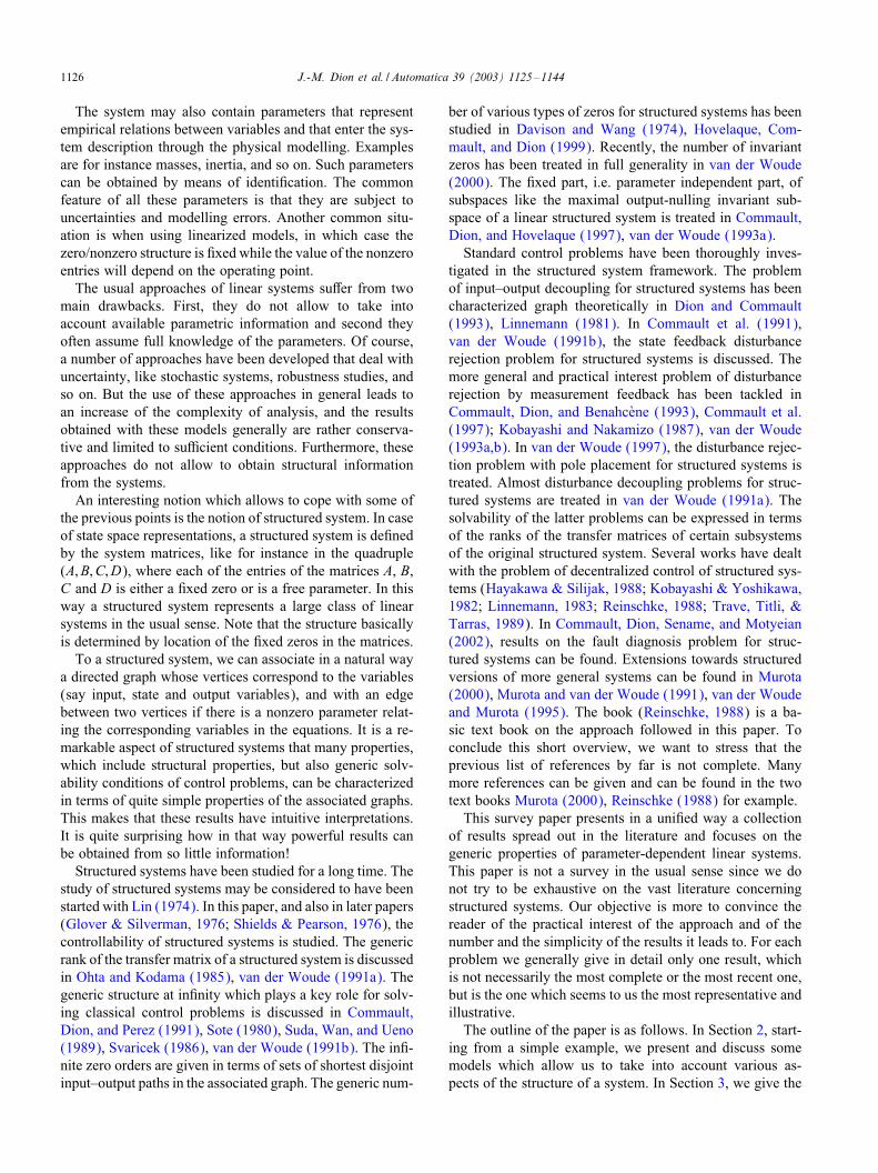
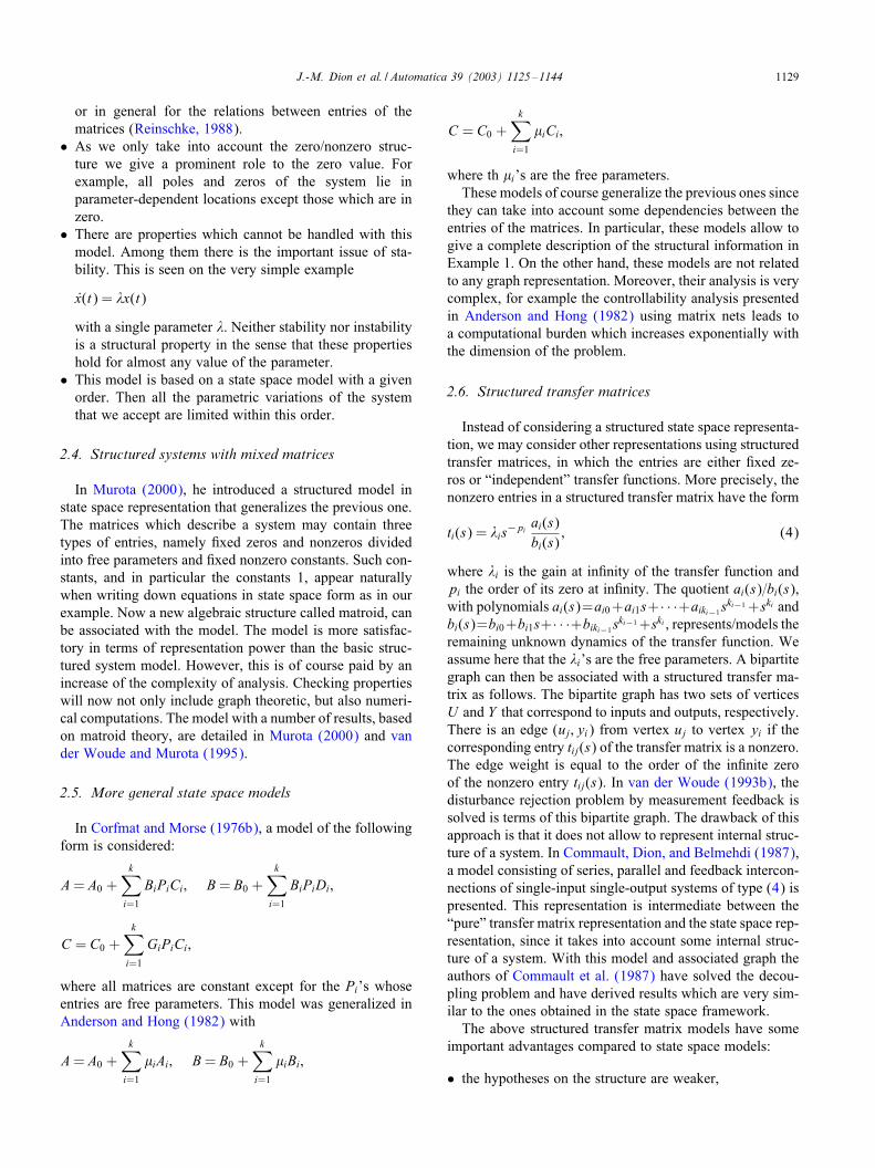
where the �i’s are the new parameters. To such a modelwe can associate in a natural way a directed graph. In this
Fig. 1.
graph, the vertices correspond to the variables (inputs, states,outputs) and the edges to the relations between variables,indeed each edge is associated with a parameter in the aboverepresentation. For the example we get the graph of Fig. 1.This graph has the advantage to clearly visualize the de-
pendence between variables in the system. Moreover, this(unweighted) graph contains the same information as thestructured matrices (A; B; C). Then the properties of the sys-tem which depend only on the zero/nonzero structure of thesystem may as well be studied on this graph. With this re-mark and using the power of graph theory, a lot of propertiesof the system can be translated into graph conditions. Thesegraph conditions are generally very intuitive and informa-tive on the system. Most of the remaining part of the paperis dedicated to this kind of results. We can summarize theinterest of this model as follows:
• The model captures an essential part of the structure, i.e.the zero/nonzero structure. A structured model representsthe class of systems which have the same zero/nonzerostructure. An important class of applications is the use inlinearized models. In this case, the zero/nonzero structureis 1xed and the value of the nonzero entries depends onthe operating point (Morari & Stephanopoulos, 1980).
• The associated graph contains all the information on themodel.
• There is a huge amount of interesting results availablein the literature using this model, they concern proper-ties and control of such systems. These results, generallyexpressed in terms of the associated graph, are often in-tuitive and easy to interpret physically.
• The conditions are expressed in graph terms and it turnsout that they can be checked by very eDcient polynomialalgorithms. This can be regarded special since in generalchecking graph conditions may be NP-hard.
The simplicity of the model is of course also paid by somedrawbacks:
• Some aspects of the structure, which may stronglyinRuence the properties of the system, are completelyignored. This is the case for the nonzero 1xed entries,
J.-M. Dion et al. / Automatica 39 (2003) 1125–1144 1129
or in general for the relations between entries of thematrices (Reinschke, 1988).
• As we only take into account the zero/nonzero struc-ture we give a prominent role to the zero value. Forexample, all poles and zeros of the system lie inparameter-dependent locations except those which are inzero.
• There are properties which cannot be handled with thismodel. Among them there is the important issue of sta-bility. This is seen on the very simple example
x(t) = �x(t)
with a single parameter �. Neither stability nor instabilityis a structural property in the sense that these propertieshold for almost any value of the parameter.
• This model is based on a state space model with a givenorder. Then all the parametric variations of the systemthat we accept are limited within this order.
2.4. Structured systems with mixed matrices
In Murota (2000), he introduced a structured model instate space representation that generalizes the previous one.The matrices which describe a system may contain threetypes of entries, namely 1xed zeros and nonzeros dividedinto free parameters and 1xed nonzero constants. Such con-stants, and in particular the constants 1, appear naturallywhen writing down equations in state space form as in ourexample. Now a new algebraic structure called matroid, canbe associated with the model. The model is more satisfac-tory in terms of representation power than the basic struc-tured system model. However, this is of course paid by anincrease of the complexity of analysis. Checking propertieswill now not only include graph theoretic, but also numeri-cal computations. The model with a number of results, basedon matroid theory, are detailed in Murota (2000) and vander Woude and Murota (1995).
2.5. More general state space models
In Corfmat and Morse (1976b), a model of the followingform is considered:
A= A0 +k∑i=1
BiPiCi; B= B0 +k∑i=1
BiPiDi;
C = C0 +k∑i=1
GiPiCi;
where all matrices are constant except for the Pi’s whoseentries are free parameters. This model was generalized inAnderson and Hong (1982) with
A= A0 +k∑i=1
�iAi; B= B0 +k∑i=1
�iBi;
C = C0 +k∑i=1
�iCi;
where th �i’s are the free parameters.These models of course generalize the previous ones since
they can take into account some dependencies between theentries of the matrices. In particular, these models allow togive a complete description of the structural information inExample 1. On the other hand, these models are not relatedto any graph representation. Moreover, their analysis is verycomplex, for example the controllability analysis presentedin Anderson and Hong (1982) using matrix nets leads toa computational burden which increases exponentially withthe dimension of the problem.
2.6. Structured transfer matrices
Instead of considering a structured state space representa-tion, we may consider other representations using structuredtransfer matrices, in which the entries are either 1xed ze-ros or “independent” transfer functions. More precisely, thenonzero entries in a structured transfer matrix have the form
ti(s) = �is−piai(s)bi(s)
; (4)
where �i is the gain at in1nity of the transfer function andpi the order of its zero at in1nity. The quotient ai(s)=bi(s),with polynomials ai(s)=ai0+ai1s+· · ·+aiki−1s
ki−1 +ski andbi(s)=bi0+bi1s+· · ·+biki−1s
ki−1+ski , represents/models theremaining unknown dynamics of the transfer function. Weassume here that the �i’s are the free parameters. A bipartitegraph can then be associated with a structured transfer ma-trix as follows. The bipartite graph has two sets of verticesU and Y that correspond to inputs and outputs, respectively.There is an edge (uj; yi) from vertex uj to vertex yi if thecorresponding entry tij(s) of the transfer matrix is a nonzero.The edge weight is equal to the order of the in1nite zeroof the nonzero entry tij(s). In van der Woude (1993b), thedisturbance rejection problem by measurement feedback issolved is terms of this bipartite graph. The drawback of thisapproach is that it does not allow to represent internal struc-ture of a system. In Commault, Dion, and Belmehdi (1987),a model consisting of series, parallel and feedback intercon-nections of single-input single-output systems of type (4) ispresented. This representation is intermediate between the“pure” transfer matrix representation and the state space rep-resentation, since it takes into account some internal struc-ture of a system. With this model and associated graph theauthors of Commault et al. (1987) have solved the decou-pling problem and have derived results which are very sim-ilar to the ones obtained in the state space framework.The above structured transfer matrix models have some
important advantages compared to state space models:
• the hypotheses on the structure are weaker,
1130 J.-M. Dion et al. / Automatica 39 (2003) 1125–1144
• the 1nite poles and zeros of the individual transfer func-tions are not relevant and may be dependent,
• a structured transfer matrix model represents a muchlarger class of structured systems than the one introducedearlier in this paper, since the McMillan degree of thesystems is not a priori 1xed.
In the next sections, we will focus our interest on the typeof the structured model presented in Section 2.3, becausethis type of model is easy to handle and frequently used inliterature.
3. Mathematical description and preliminaries
3.1. Structured systems
We study linear time-invariant systems of the followingform:
":x(t) = Ax(t) + Bu(t);
y(t) = Cx(t) + Du(t);(5)
where x(t)∈Rn denotes the state of the system, u(t)∈Rm
the input and y(t)∈Rp the output. As indicated, the vectorsx; u and y all depend on the time t, but this dependency willbe omitted in the notation in the remainder. The matricesA; B; C and D are real valued matrices of suitable dimen-sions.In this paper, we assume that we only know the struc-
ture of the matrices A; B; C and D. By this we mean thatwe know which entries in the matrices are 1xed to zero,and consequently which entries are not 1xed to zero. In theremainder, the latter nonzero entries are referred to as thenonzeros. Besides the zero/nonzero information, we assumein this paper that the actual value of each of the nonzerosis unknown too. In fact, we assume that the nonzeros canattain any real value, including possibly even zero. We cantherefore parametrize each nonzero by means of a real scalarparameter. Then, if the system has f nonzeros, it can beparametrized by means of a parameter vector �∈% = Rf.The set of parametrized systems thus obtained is referred toas a structured system and is denoted by
"�:x(t) = A�x(t) + B�u(t);
y(t) = C�x(t) + D�u(t)(6)
with �∈%. For each value of � system (6) is completelyknown. In this paper, we refer to such a completely knownsystem as a system of type (5), whereas a structured systemwill be denoted as a system of type (6) with � unspeci1ed.
3.2. Generic properties
By choosing �∈%, system (6) becomes completelyknown and can be written as a system of the form (5).Hence, for each value of �∈% system theoretic propertiescan be studied in the normal way. However, it is clear that
the properties do depend on the chosen parameter value.For some values a property may be true, while for othervalues not. For a number of system theoretic properties,however it turns out that once a property is true for oneparameter value, it is true for almost all parameter values.Here “for almost all parameter values” is to be understoodas “for all parameter values except for those in some properalgebraic variety in the parameter space %”. The properalgebraic variety for which a property is not true is the zeroset of some nontrivial polynomial with real coeDcients inthe f parameters of the system, which can be written downexplicitly, i.e. we can precisely describe when a propertyfails to be true. A proper algebraic variety has Lebesguemeasure zero. Therefore, a property which is true for almostall parameter values, is also often said to be true generically(Davison & Wang, 1973).
3.3. Graph of a structured system
Structured systems can be represented elegantly by meansof directed graphs. Using such type of representation, itis possible to study well-known system theoretic proper-ties from a graph theoretic point of view. The results ofthese studies are conditions that only depend on the struc-ture/the graph of the system, and therefore, besides excep-tional cases, do not depend on the numerical values of theparameters of the system, i.e. the values of the nonzeros inthe matrices describing the system.The graph G = (V; E) of a structured system of type (6)
is de1ned by a vertex set V and an edge set E. The vertexset V is given by U ∪ X ∪ Y with U = {u1; : : : ; um} the setof input vertices, X = {x1; : : : ; xn} the set of state vertices,Y = {y1; : : : ; yp} the set of output vertices. Denoting (v; v′)for a directed edge from the vertex v∈V to the vertex v′ ∈V ,the edge set E is described by EA ∪ EB ∪ EC ∪ ED withEA = {(xj; xi)|A�; ij = 0}, EB = {(uj; xi)|B�; ij = 0}, EC ={(xj; yi)|C�; ij = 0} and ED = {(uj; yi)|D�;ij = 0}. In thelatter, for instance A�; ij = 0 means that the (i; j)th entry ofthe matrix A� is a parameter (a nonzero). An example of thegraph of a structured system is given below.
3.4. Example of graph of a structured system
Consider structured system (6) described by the matrices
A� =
0 0 0
�1 0 0
0 0 0
; B� =
�2 0
0 0
0 �3
;
C� =
(0 �4 0
0 0 �5
); D� =
(0 �6
0 0
):
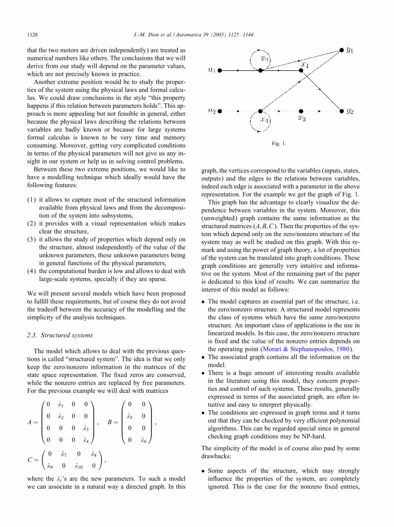
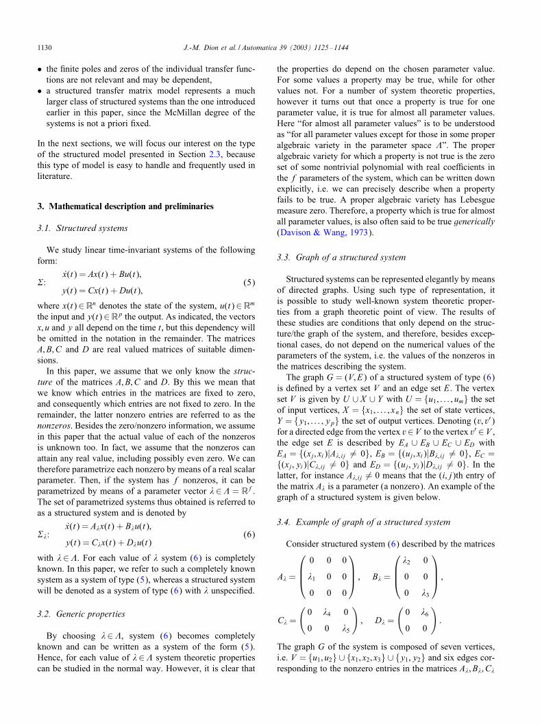
The graph G of the system is composed of seven vertices,i.e. V = {u1; u2} ∪ {x1; x2; x3} ∪ {y1; y2} and six edges cor-responding to the nonzero entries in the matrices A�; B�; C�
J.-M. Dion et al. / Automatica 39 (2003) 1125–1144 1131
Fig. 2.
and D�. For example the edge (x1; x2) is associated with theparameter �1 in A� and the edge (u2; y1) is associated withthe parameter �6 in D�. The resulting graph can be depictedas in Fig. 2.
3.5. Linkings, cycle families, strong components
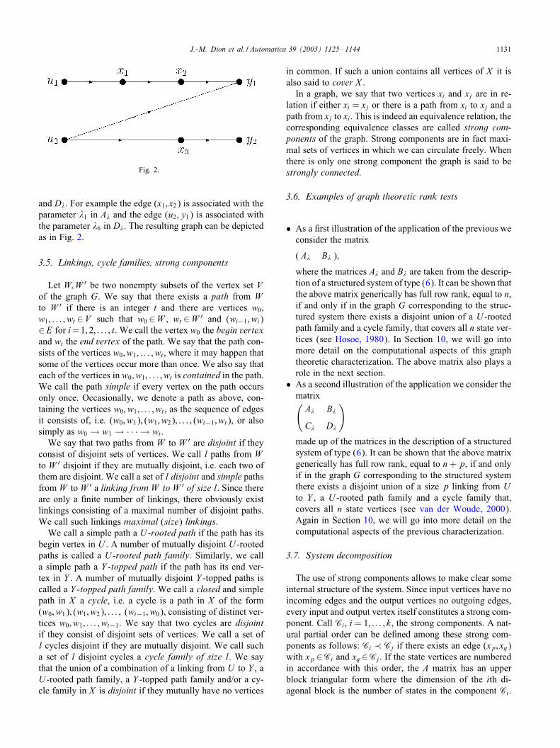
Let W;W ′ be two nonempty subsets of the vertex set Vof the graph G. We say that there exists a path from Wto W ′ if there is an integer t and there are vertices w0;w1; : : : ; wt ∈V such that w0 ∈W , wt ∈W ′ and (wi−1; wi)∈E for i=1; 2; : : : ; t. We call the vertex w0 the begin vertexand wt the end vertex of the path. We say that the path con-sists of the vertices w0; w1; : : : ; wt , where it may happen thatsome of the vertices occur more than once. We also say thateach of the vertices in w0; w1; : : : ; wt is contained in the path.We call the path simple if every vertex on the path occursonly once. Occasionally, we denote a path as above, con-taining the vertices w0; w1; : : : ; wt , as the sequence of edgesit consists of, i.e. (w0; w1); (w1; w2); : : : ; (wt−1; wt), or alsosimply as w0 → w1 → · · · → wt .We say that two paths from W to W ′ are disjoint if they
consist of disjoint sets of vertices. We call l paths from Wto W ′ disjoint if they are mutually disjoint, i.e. each two ofthem are disjoint. We call a set of l disjoint and simple pathsfromW toW ′ a linking from W to W ′ of size l. Since thereare only a 1nite number of linkings, there obviously existlinkings consisting of a maximal number of disjoint paths.We call such linkings maximal (size) linkings.We call a simple path a U -rooted path if the path has its
begin vertex in U . A number of mutually disjoint U -rootedpaths is called a U -rooted path family. Similarly, we calla simple path a Y -topped path if the path has its end ver-tex in Y . A number of mutually disjoint Y -topped paths iscalled a Y -topped path family. We call a closed and simplepath in X a cycle, i.e. a cycle is a path in X of the form(w0; w1); (w1; w2); : : : ; (wt−1; w0), consisting of distinct ver-tices w0; w1; : : : ; wt−1. We say that two cycles are disjointif they consist of disjoint sets of vertices. We call a set ofl cycles disjoint if they are mutually disjoint. We call sucha set of l disjoint cycles a cycle family of size l. We saythat the union of a combination of a linking from U to Y , aU -rooted path family, a Y -topped path family and/or a cy-cle family in X is disjoint if they mutually have no vertices
in common. If such a union contains all vertices of X it isalso said to cover X .In a graph, we say that two vertices xi and xj are in re-
lation if either xi = xj or there is a path from xi to xj and apath from xj to xi. This is indeed an equivalence relation, thecorresponding equivalence classes are called strong com-ponents of the graph. Strong components are in fact maxi-mal sets of vertices in which we can circulate freely. Whenthere is only one strong component the graph is said to bestrongly connected.
3.6. Examples of graph theoretic rank tests
• As a 1rst illustration of the application of the previous weconsider the matrix
( A� B� );
where the matrices A� and B� are taken from the descrip-tion of a structured system of type (6). It can be shown thatthe above matrix generically has full row rank, equal to n,if and only if in the graph G corresponding to the struc-tured system there exists a disjoint union of a U -rootedpath family and a cycle family, that covers all n state ver-tices (see Hosoe, 1980). In Section 10, we will go intomore detail on the computational aspects of this graphtheoretic characterization. The above matrix also plays arole in the next section.
• As a second illustration of the application we consider thematrix(A� B�
C� D�
)
made up of the matrices in the description of a structuredsystem of type (6). It can be shown that the above matrixgenerically has full row rank, equal to n+p, if and onlyif in the graph G corresponding to the structured systemthere exists a disjoint union of a size p linking from Uto Y , a U -rooted path family and a cycle family that,covers all n state vertices (see van der Woude, 2000).Again in Section 10, we will go into more detail on thecomputational aspects of the previous characterization.
3.7. System decomposition
The use of strong components allows to make clear someinternal structure of the system. Since input vertices have noincoming edges and the output vertices no outgoing edges,every input and output vertex itself constitutes a strong com-ponent. Call Ci, i= 1; : : : ; k, the strong components. A nat-ural partial order can be de1ned among these strong com-ponents as follows: Ci ≺ Cj if there exists an edge (xp; xq)with xp ∈Ci and xq ∈Cj. If the state vertices are numberedin accordance with this order, the A matrix has an upperblock triangular form where the dimension of the ith di-agonal block is the number of states in the component Ci.
1132 J.-M. Dion et al. / Automatica 39 (2003) 1125–1144
When the part of the graph corresponding to state verticesis strongly connected, matrix A is said to be irreducible.To the initial graph we can associate another graph, called
condensed graph, in which a vertex corresponds to a strongcomponent, and there is an edge between two vertices ifthere is an edge between two vertices of the correspondingstrong components in the initial graph. There are qualitativeproperties of the original graph, in particular reachabilityproperties, which can be studied on the condensed graph.This may considerably reduce the complexity of analysis ofthe system (see Jantzen, 1994).
4. Controllability
In this section, we treat controllability for structured sys-tems of type (6). The results of this section are well-knownand can be found in for instance Glover & Silverman (1976),Lin (1974), Reinschke (1988), Shields and Pearson (1976).
4.1. DeBnitions
In order to present results on generic controllability weneed some additional de1nitions.The notion of controllability for completely speci1ed sys-
tems of type (5) is well-known. For this we refer to manytextbooks on system theory that are available. As for eachchoice of �∈% a system of type (6) is completely known,it consequently can be checked for controllability for each�∈%. It turns out that once a structured system is control-lable for one choice of �∈%, it is controllable for almostall �∈%, in which case the structured system then will besaid to be generically controllable.A structured system of type (6) is said to be reducible, or
to be in form I, if there exists a permutation matrix P, withPT denoting the transpose of P, such that
PTA�P =
(A�;11 0
A�;21 A�;22
); PTB� =
(0
B�;2
);
where A�; ij is an ni × nj matrix for appropriate i; j = 1; 2,with 0¡n16 n and n1+n2=n, and where B�;2 is an n2×mmatrix. A structured system of type (6) is said to be notof full generic row rank, or to be in form II, if the genericrank of (A� B�) is less than n. Recall that the latter can beexpressed in terms of graphs as explained in the previoussection.In the graph of a structured system, a bud is an elementary
cycle in X with an additional edge that ends, but not begins,in a vertex of the cycle. The begin vertex of the edge is thenalso said to be the begin vertex of the bud. A stem is anelementary path starting in U . A cactus is a subgraph that isde1ned recursively as follows. A cactus C is either a stem,or is obtained from a smaller cactus C′, to which a bud hasbeen added that is vertex disjoint from C′ apart from the
begin vertex of the bud, which can be any vertex of C′,except for the last vertex of the stem that is contained in C′.
4.2. Structural controllability
For structured systems of type (6), the following resultshave been proved (see Glover & Silverman, 1976; Lin, 1974;Reinschke, 1988; Shields & Pearson, 1976).
Theorem 1. The next statements for a structured systemof type (6) with a graph G are equivalent.
a. The structured system is generically controllable.b. The structured system is neither in form I nor in form
II.c. In G there exists a vertex disjoint union of cacti that
covers all state vertices.d. In G every state vertex is the end vertex of a U -rooted
path and there exists a disjoint union of aU -rooted pathfamily and a cycle family that covers all state vertices.
This theorem allows to check the structural (generic) con-trollability of the system on the associated graph. Note thatsimilar graph results hold for structural observability.
4.3. Examples with generic controllability
We consider a structured system of type (6) with
A� =
(0 0
0 0
); B� =
(�1
�2
)
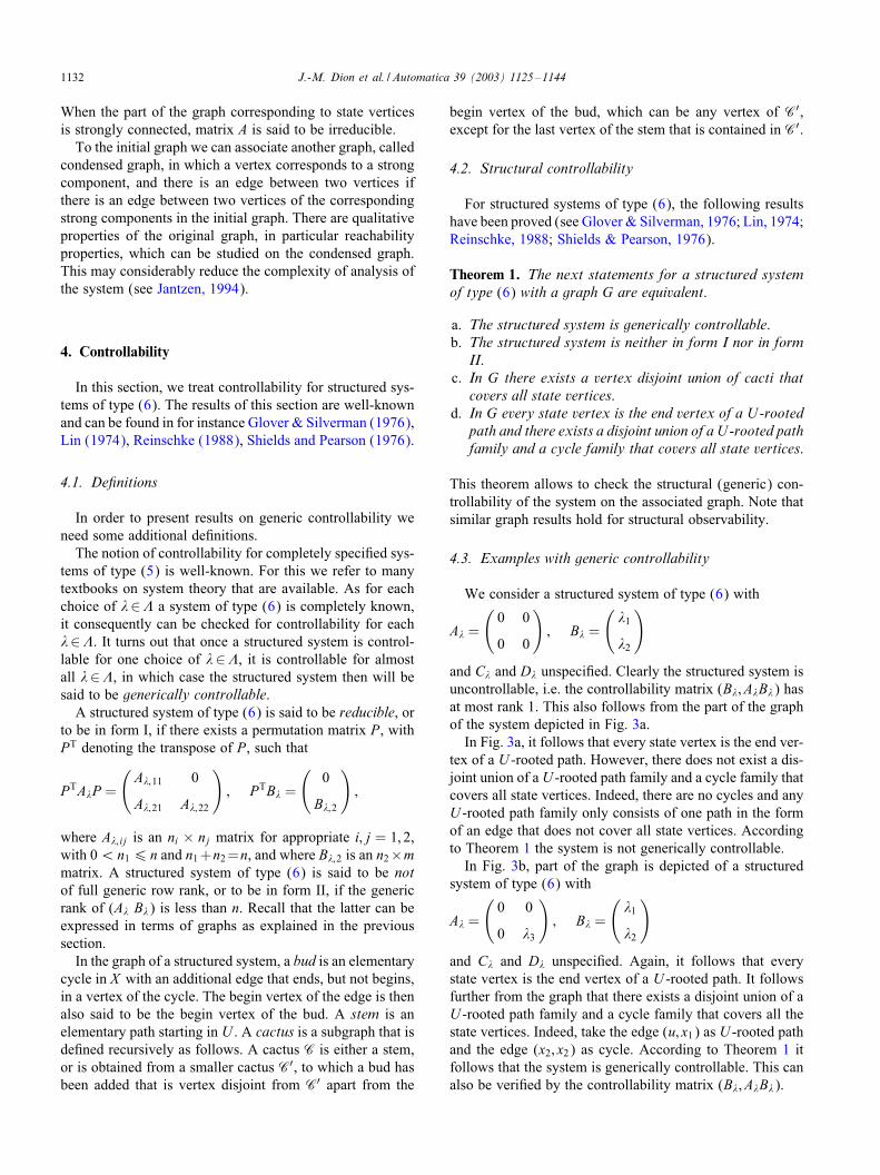
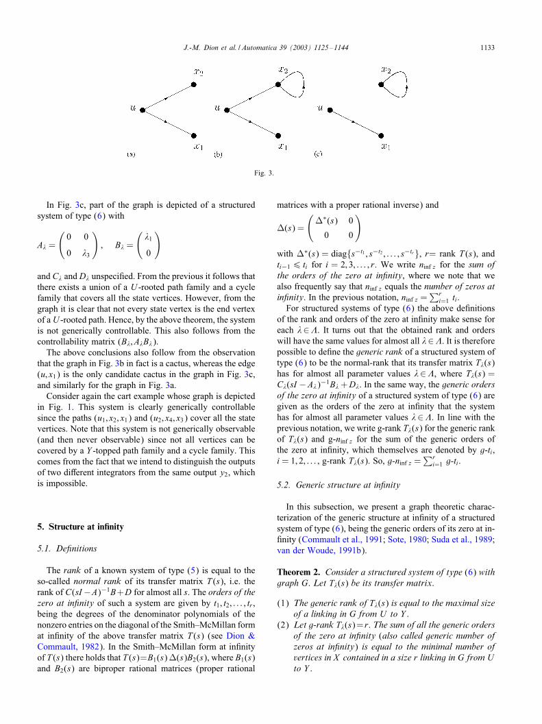
and C� and D� unspeci1ed. Clearly the structured system isuncontrollable, i.e. the controllability matrix (B�; A�B�) hasat most rank 1. This also follows from the part of the graphof the system depicted in Fig. 3a.In Fig. 3a, it follows that every state vertex is the end ver-
tex of a U -rooted path. However, there does not exist a dis-joint union of a U -rooted path family and a cycle family thatcovers all state vertices. Indeed, there are no cycles and anyU -rooted path family only consists of one path in the formof an edge that does not cover all state vertices. Accordingto Theorem 1 the system is not generically controllable.In Fig. 3b, part of the graph is depicted of a structured
system of type (6) with
A� =
(0 0
0 �3
); B� =
(�1
�2
)
and C� and D� unspeci1ed. Again, it follows that everystate vertex is the end vertex of a U -rooted path. It followsfurther from the graph that there exists a disjoint union of aU -rooted path family and a cycle family that covers all thestate vertices. Indeed, take the edge (u; x1) as U -rooted pathand the edge (x2; x2) as cycle. According to Theorem 1 itfollows that the system is generically controllable. This canalso be veri1ed by the controllability matrix (B�; A�B�).
J.-M. Dion et al. / Automatica 39 (2003) 1125–1144 1133
Fig. 3.
In Fig. 3c, part of the graph is depicted of a structuredsystem of type (6) with
A� =
(0 0
0 �3
); B� =
(�1
0
)
and C� and D� unspeci1ed. From the previous it follows thatthere exists a union of a U -rooted path family and a cyclefamily that covers all the state vertices. However, from thegraph it is clear that not every state vertex is the end vertexof aU -rooted path. Hence, by the above theorem, the systemis not generically controllable. This also follows from thecontrollability matrix (B�; A�B�).The above conclusions also follow from the observation
that the graph in Fig. 3b in fact is a cactus, whereas the edge(u; x1) is the only candidate cactus in the graph in Fig. 3c,and similarly for the graph in Fig. 3a.Consider again the cart example whose graph is depicted
in Fig. 1. This system is clearly generically controllablesince the paths (u1; x2; x1) and (u2; x4; x3) cover all the statevertices. Note that this system is not generically observable(and then never observable) since not all vertices can becovered by a Y -topped path family and a cycle family. Thiscomes from the fact that we intend to distinguish the outputsof two diCerent integrators from the same output y2, whichis impossible.
5. Structure at in�nity
5.1. DeBnitions
The rank of a known system of type (5) is equal to theso-called normal rank of its transfer matrix T (s), i.e. therank of C(sI−A)−1B+D for almost all s. The orders of thezero at inBnity of such a system are given by t1; t2; : : : ; tr ,being the degrees of the denominator polynomials of thenonzero entries on the diagonal of the Smith–McMillan format in1nity of the above transfer matrix T (s) (see Dion &Commault, 1982). In the Smith–McMillan form at in1nityof T (s) there holds that T (s)=B1(s)S(s)B2(s), where B1(s)and B2(s) are biproper rational matrices (proper rational
matrices with a proper rational inverse) and
S(s) =
(S∗(s) 0
0 0
)
with S∗(s) = diag{s−t1 ; s−t2 ; : : : ; s−tr}, r= rank T (s), andti−16 ti for i = 2; 3; : : : ; r. We write ninf z for the sum ofthe orders of the zero at inBnity, where we note that wealso frequently say that ninf z equals the number of zeros atinBnity. In the previous notation, ninf z =
∑ri=1 ti.
For structured systems of type (6) the above de1nitionsof the rank and orders of the zero at in1nity make sense foreach �∈%. It turns out that the obtained rank and orderswill have the same values for almost all �∈%. It is thereforepossible to de1ne the generic rank of a structured system oftype (6) to be the normal-rank that its transfer matrix T�(s)has for almost all parameter values �∈%, where T�(s) =C�(sI −A�)−1B�+D�. In the same way, the generic ordersof the zero at inBnity of a structured system of type (6) aregiven as the orders of the zero at in1nity that the systemhas for almost all parameter values �∈%. In line with theprevious notation, we write g-rank T�(s) for the generic rankof T�(s) and g-ninf z for the sum of the generic orders ofthe zero at in1nity, which themselves are denoted by g-ti,i = 1; 2; : : : ; g-rank T�(s). So, g-ninf z =
∑ri=1 g-ti.
5.2. Generic structure at inBnity
In this subsection, we present a graph theoretic charac-terization of the generic structure at in1nity of a structuredsystem of type (6), being the generic orders of its zero at in-1nity (Commault et al., 1991; Sote, 1980; Suda et al., 1989;van der Woude, 1991b).
Theorem 2. Consider a structured system of type (6) withgraph G. Let T�(s) be its transfer matrix.
(1) The generic rank of T�(s) is equal to the maximal sizeof a linking in G from U to Y .
(2) Let g-rank T�(s)= r. The sum of all the generic ordersof the zero at inBnity (also called generic number ofzeros at inBnity) is equal to the minimal number ofvertices in X contained in a size r linking in G from Uto Y .
1134 J.-M. Dion et al. / Automatica 39 (2003) 1125–1144
(3) Let g-rank T (s) = r and let 2i be the minimal numberof vertices in X contained in a size i linking in G fromU to Y for i = 1; 2; : : : ; r. Then the generic orders ofthe zeros at inBnity of the system are given by the listg-linf z = {g-ti|i = 1; : : : ; r}, where g-ti = 2i − 2i−1 fori=1; 2; : : : ; r, with 20 =0. Clearly,
∑ri=1 g-ti=g-ninf z.
Consider the example in Section 3.4 with a graph G asdepicted in Fig. 2. From the graph G, it is clear that themaximal number of disjoint paths from U ={u1; u2} to Y ={y1; y2} is equal to 2. Indeed, consider the two paths u1 →x1 → x2 → y1 and u2 → x3 → y2. Clearly, this set of twopaths is the only possibility for a size 2 linking from U toY . Hence, the minimal number of vertices in X covered bya size 2 linking from U to Y is 3. From the graph it furtherfollows that the minimal number of vertices in X coveredby a size 1 linking (a single path) from U to Y is 0. Forthis consider the path given by the edge (u2; y1). In terms ofthe notation in Theorem 2 it follows that 21 = 0 and 22 = 3.From Theorem 2, it therefore follows that the generic rankof the structured system in Section 3.4 is equal to 2, and thegeneric orders of its zero at in1nity are given by 0 and 3.The previous conclusions can also be veri1ed directly
from the transfer matrix of the structured system in Section3.4. This transfer matrix equals
T�(s) =
�1�2�4s2
�6
0�3�5s
:
The matrix T�(s) clearly has rank 2, for almost all parametervalues. Hence, g-rank T�(s) = 2. Furthermore, it follows bystraightforward calculation that
1�6
0
−�3�5�6s
1
�1�2�4s2
�6
0�3�5s
0 − �6�1�2�3�4�5
11
�3�5s2
=
1 0
01s3
:
Note that the left and right factors in the left-hand side ofthe equality generically are biproper rational matrices. So, itfollows that generically the zero at in1nity has orders 0 and3, i.e. g-t1=0 and g-t2=3, and that consequently g-ninf z=3.By this the statements in Theorem 2 have been illustratedagain.
6. Finite structure
6.1. DeBnitions
We 1rst consider a known system of type (5). The follow-ing subspaces are well-known and play a prominent role in
the geometric approach towards system theory (see Aling &Schumacher, 1984; Basile &Marro, 1969; Wonham, 1985).
• Themaximal output-nulling invariant subspaceV∗ is themaximal subspace V for which there exists a feedbackmatrix F such that (A + BF)V ⊂ V ⊂ Ker(C + DF).Here maximal is to be seen in subspace inclusion sense.This subspace is also called the maximal (A; B)-invariantsubspace contained in Ker(C + DF).
• The maximal output-nulling controllability subspace R∗
is the maximal subspace R such that for any x0; x1 ∈Rthere exists a time t1¿ 0 and a control (function) u(t) fort¿ 0; such that x(0) = x0; x(t1) = x1, while y(t) = 0 forall t with 06 t6 t1.
In system theory the notion of invariant zero plays an im-portant role. Invariant zeros are the zeros of the nonzeropolynomials on the diagonal of the Smith form of the sys-tem pencil
P(s) =
(A− sI B
C D
):
We write ninv z for the number of invariant zeros where wecount the multiplicity.For structured systems of type (6) the above makes sense
for each individual �∈%. In fact, we can even talk aboutthe generic number of invariant zeros of a structured systemas the number of invariant zeros that the structured systemhas for almost all �∈%. We write g-ninv z for the genericnumber of invariant zeros where we count the multiplicity.It turns out that we can make a distinction between invariantzeros that are located at s = 0 and invariant zeros that arelocated outside s = 0. It can be shown that the latter aremutually distinct, while the former can occur with one ormore nonnegative orders. This is analogous to zero at in1nitywhich also can occur with one or more nonnegative orders.We will go deeper into this matter in Section 6.2.In the proposition below, we recall two well-known re-
lations between the numbers of the two types of zeros in-troduced up to now, i.e. invariant zeros and zero at in1n-ity, and the dimensions of the two maximal invariant sub-spaces de1ned above. (See also Aling & Schumacher, 1984;Rosenbrock, 1970).
Proposition 3. Given a known system of type (5).
(1) dimV∗ = n − ninf z, whenever the system pencil P(s)is right invertible,
(2) dimR∗ = dimV∗ − ninv z.
For structured systems of type (6) generic versions of theabove relations follow directly, i.e.
1. g-dimV∗�=n−g-ninf z, whenever the system pencil P�(s)
is generically right invertible,2. g-dimR∗
� = g-dimV∗� − g-ninv z,
J.-M. Dion et al. / Automatica 39 (2003) 1125–1144 1135
where P�(s) denotes the pencil of the structured systemparametrized by �, i.e.
P�(s) =
(A� − sI B�
C� D�
);
which is said to be generically right invertible if P�(s) isright invertible for almost all �∈%. Further, g-dimV∗
� de-notes the generic dimension of V∗
� , i.e. the dimension thatthe maximal output-nulling subspace corresponding to struc-tured system (6) has for almost all �∈%. Likewise forg-dimR∗
� .Like the spaces themselves, also their generic dimensions
play a prominent role for structured systems. By the above itis clear how, for the case that the system generically is rightinvertible, the generic dimensions of V∗
� and R∗� can be
obtained from the generic number of invariant zeros and thesum of the generic orders of the zero at in1nity. In Section5, we presented how the sum of the generic orders of zero atin1nity of a structured system, i.e. g-ninf z, can be determinedfrom the graph G of the system. The determination of thegeneric number of invariant zeros is not that easy, exceptfrom some special cases which are presented below.
6.2. Generic number of invariant zeros
We start this section by presenting graph theoretic char-acterizations of the generic number of invariant zeros of astructured system for some special cases. For proofs werefer to van der Woude (2000).
Theorem 4. Let a linear structured system of type (6) withgraph G be given.
(1) Letm=p and g-rank T (s)=p (system"� is square andgenerically invertible). The generic number of invari-ant zeros of system "� is equal to n minus its genericnumber of zeros at inBnity, i.e. n minus the minimalnumber of vertices in X contained in a size p linkingfrom U to Y .
(2) Let g-rank P(s) = n + p, even after the deletion ofan arbitrary column from P(s). Then generically theinvariant zeros of system "� are all located at s=0 andtheir generic number is equal to n minus the maximalnumber of vertices in X contained in the disjoint unionof a size p linking from U to Y , a cycle family in Xand a U -rooted path family.
In van der Woude (2000), it is proved that any structuredsystem can be decomposed in three subsystems. The pencilof the 1rst subsystem is full row rank even after the dele-tion of an arbitrary column, the second subsystem is squareinvertible and the pencil of the third one is full column rankeven after the deletion of an arbitrary row. Using this de-composition and the above theorem enables us to computethe total number of invariant zeros, the complete structureof the zero in s=0 and the dimensions of V∗
� and R∗� in the
Fig. 4.
general case, see van der Woude (2000) and van der Woudeet al. (2000) for details.
6.3. Example of computation of the generic structure
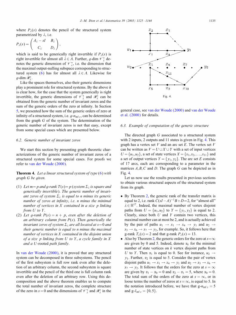
The directed graph G associated to a structured systemwith 2 inputs, 2 outputs and 11 states is given in Fig. 4. Thisgraph has a vertex set V and an arc set E. The vertex set Vcan be written as V =U ∪X ∪Y with a set of input verticesU ={u1; u2}, a set of state vertices X ={x1; x2; : : : ; x11} anda set of output vertices Y = {y1; y2}. The arc set E consistsof 17 arcs, each arc corresponding to a parameter in thematrices A; B; C and D. The graph G can be depicted as inFig. 4.Let us now use the results presented in previous sections
to obtain various structural aspects of the structured systemfrom its graph.
• By Theorem 2, the generic rank of the transfer matrix isequal to 2, i.e. rank C(sI−A)−1B+D=2, for “almost all”�∈R17. Indeed, the maximal number of vertex disjointpaths from U = {u1; u2} to Y = {y1; y2} is equal to 2.Clearly, since both U and Y contain two vertices, thismaximal number can at most be 2, and is actually achievedby the pair of paths u1 → x1 → x4 → y1 and u2 →x5 → x6 → x7 → y2, for example. So, it follows here thatg-rank T�(s) = 2 and that g-rank P�(s) = 13.
• Also by Theorem 2, the generic orders for the zero at s=∞are given by 0 and 5. Indeed, denote 2k for the minimalnumber of state vertices on k vertex disjoint paths fromU to Y . Then 21 is equal to 0. See for instance, u2 →y1. Further, 22 is equal to 5. Consider the pair of vertexdisjoint paths u1 → x1 → x4 → y1 and u2 → x5 → x6 →x7 → y2. It follows that the orders for the zero at s=∞are given by 21 − 20 = 0 and 22 − 21 = 5, where 20 = 0.The total sum of the orders of the zero at s = ∞, or inloose terms the number of zeros at s=∞, is equal to 5. Inthe notation introduced before, we have that g-ninf z = 5and g-linf z = {0; 5}.

1136 J.-M. Dion et al. / Automatica 39 (2003) 1125–1144
• By Theorem 4, if a system is square and generically in-vertible, the generic number of invariant zeros can be ob-tained by subtracting the sum of the orders of the zerosat s=∞ from the state space dimension. Here this yieldsthat there are 11−5=6 invariant zeros. Using the resultsof van der Woude et al. (2000) it is possible to prove thatthe generic invariant zero orders at s = 0 are 1 and 3. Itfollows that there are two invariant zeros outside s = 0.As mentioned before, it can be shown that these latter twozeros generically are mutually distinct.
7. Decoupling and disturbance rejection
In this section, we revisit some classical feedback con-trol problems in our framework of structured systems. Ourpurpose is to answer the question whether or not these clas-sical control problems generically have a solution. It turnsout that for some of these problems this question can be an-swered by verifying some simple graph theoretic conditions.If the answer is yes, then classical synthesis methods haveto be applied to obtain a practical solution. If the answer isno, the graph theoretic analysis tells us where the bottleneckof the problem is located.Most of the problems tackled below received a complete
solution in the early seventies. The systems were supposedto be known and the solutions were expressed in algebraicor geometric terms. The original solvability conditions weresimpli1ed in the eighties and were expressed in terms ofthe in1nite structure of linear systems. Using the results ofthe previous sections on the characterization of the in1nitestructure of linear structured systems, it is therefore possibleto derive simple graph theoretic conditions for the genericsolvability of the classical control problems studied in thissection.
7.1. State feedback decoupling
The decoupling or noninteracting control problem is oneof the most famous problems of control theory. Besides itspractical interest it has also led to a number of fundamentalresults of general interest in system theory.Let us recall the formulation of the problem (also known
as the row-by-row decoupling problem or Morgan’s prob-lem) in its simplest form for known systems. We considera system of type (5), where we assume that the system issquare, i.e. m=p, so that the system has the same number ofinputs as outputs. We look for a state feedback u=Fx+ Jv,with J nonsingular, such that the closed loop system transfermatrix
TF;J (s) = (C + DF)(sI − A− BF)−1BJ + DJ (7)
is diagonal and nonsingular. It was shown in Descusse andDion (1982) that this problem has a solution if and onlyif the in1nite structure of the system coincides with theunion of the in1nite structures of the p subsystems obtained
by focusing on each output component individually as theoutput of a subsystem. In the framework of linear structuredsystems, the formulation of the generic problem and theprevious result can be combined in a natural way. After somesimpli1cation the result can be stated as in the followingtheorem (Dion & Commault, 1993; Linnemann, 1981).
Theorem 5. Consider a structured system of type (6) withgraph G and with m = p. The state feedback decouplingproblem is generically solvable if and only if
(1) There exists a size m linking L in G from U to Y , and(2) Lm =
∑mi=1 L
(i)1 , where Lm is the minimal number of
vertices in X contained in a size m linking in G fromU to Y , and L(i)1 is the minimal number of vertices inX contained in a size 1 linking (a path) in G from Uto the output vertex set {yi}.
In alternative terms, Theorem 5 simply says that the decou-pling problem has a solution if and only if we can 1nd asize m linking in G from U to Y such that, for any i, thepath of this linking with end vertex yi is a “minimal length”path from U to {yi}. Roughly speaking, we try to 1nd aone-to-one correspondence between inputs and outputs suchthat each input is the “closest” to its corresponding output.
7.2. Examples
Consider again the cart example described by the matrices
A=
0 �1 0 0
0 �2 0 0
0 0 0 �3
0 0 0 �4
; B=
0 0
�5 0
0 0
0 �6
;
C =
(0 �7 0 �8
�9 0 �10 0
):
The resulting graph is depicted in Fig. 1. For this exampleit can be checked easily using Theorems 2 and 4 that thegeneric rank is 2, the generic orders of the zeros at in1nityare 1 and 2 and that the system possesses generically oneinvariant zero located at s = 0. Let us consider now thisexample with respect to Theorem 5. There are two size 2linkings in G from U to Y , for example u1 → x2 → y1 andu2 → x4 → x3 → y2. The minimal number of vertices inX on a size 2 linking is equal to 3, so that L2 = 3. Thereare two size 1 linkings in G from U to {y1}. The minimalnumber of vertices in X on such linkings to y1 is equal to1, implying that L(1)1 = 1. There are two size 1 linkings in Gfrom U to {y2}. The minimal number of vertices in X onthese linkings to y2 is 2, implying that L(2)1 = 2. It followstherefore that the conditions of Theorem 5 are ful1lled and
J.-M. Dion et al. / Automatica 39 (2003) 1125–1144 1137
the system is generically decouplable. It can be checked thatwith a state feedback control u= Fx + Jv where
F =
0 −�2�5
0 0
0 0 0 −�4�6
and
J =
(�5�7 �6�8
�1�5�9 �3�6�10
)−1
;
we get the closed loop transfer matrix
T�F;J (s) =
1s
0
01s2
:
If we consider again the example in Section 3.4, there is onesize 2 linking in G from U to Y . The (minimal) number ofvertices in X on this linking is equal to 3, so that L2 = 3.There are two size 1 linkings in G from U to {y1}. Theminimal number of vertices in X on such a linking to y1 isequal to 0, implying that L(1)1 = 0. Finally, there is one size1 linking in G from U to {y2}. The (minimal) number ofvertices in X on this linking is 1, implying that L(2)1 = 1. Itfollows therefore that the second condition of Theorem 5 isnot ful1lled and the system is not generically decouplable.It should be noted that when a system is generically not
decouplable, as in the latter example, the system may bedecouplable for some values of the parameters. In the latterexample this is the case if �6 = 0.
7.3. State feedback disturbance rejection
The disturbance rejection problem received a very ele-gant solution in geometric terms (see Basile & Marro, 1969;Wonham, 1985). As for the decoupling problem, the geo-metric conditions were interpreted later in structural terms,more precisely in terms of the in1nite structure of linear sys-tems. It can be shown that the disturbance rejection prob-lem has a solution if and only if the system considering thecontrol inputs alone, and the system considering control anddisturbance inputs together, have the same in1nite structure.The latter includes that the rank of both systems is equal, asthe rank simply is the number of orders of zero at in1nity.Let us recall the statement of the problem. We consider a
known system of type (5) with an additional input q(t)∈Rd
which is called disturbance and which we would like to haveno eCect on the output.
"q:x(t) = Ax(t) + Bu(t) + Eq(t);
y(t) = Cx(t) + Du(t):(8)
We look for a state feedback u=Fx+Jq such that the closedloop system transfer matrix from disturbance to output is
equal to zero, i.e.
TF;G(s) = (C + DF)(sI − A− BF)−1(BJ + E) + DJ = 0:(9)
This problem is called the disturbance rejection problemby state feedback and disturbance measurement, where thephrase “disturbance measurement” indicates that the distur-bances are available for measurement and will be used forcontrol purposes. The problem can also be stated in thestructured system framework, where we have to deal with alinear structured system "q� described as follows:
"q�:x(t) = A�x(t) + B�u(t) + E�q(t);
y(t) = C�x(t) + D�u(t):(10)
We associate a graph Gq to the linear structured system "q�
by adding to the graph G of the original structured systema set of vertices Q corresponding to the disturbances anda set of edges corresponding to the parameters in E�. Inaddition to Gq, we also will consider the graph G of theoriginal system without disturbances, which can be seen asa subgraph of Gq. The conditions for disturbance rejectioncan now be stated in terms of the two graphs G and Gq asfollows (see Commault et al., 1991).
Theorem 6. Consider a structured system of type (10)withgraph Gq. The disturbance rejection problem by state feed-back and disturbance measurement is generically solvableif and only if
(1) A maximum size linking in G from U to Y and amaximum size linking in Gq from U ∪Q to Y have thesame size. Let this size be r.
(2) Lr=Ld;r , where Lr is the minimal number of vertices inX contained in a size r linking in G from U to Y , andLd;r is the minimal number of vertices in X containedin a size r linking in Gq from U ∪ Q to Y .
In simple words, Theorem 6 says that the disturbance rejec-tion problem with state feedback and disturbance measure-ment has a solution if and only if the control inputs are “nu-merous” and “quick enough” to compensate the inRuence ofdisturbances before they reach the outputs.In case the disturbances are not available for control pur-
poses, so that we have to take J =0, we have the followingresult.
Theorem 7. Consider a structured system of type (10)withgraph Gq. The disturbance rejection problem by state feed-back (and without disturbance measurement) is genericallysolvable if and only if
(1) A maximum size linking in G from U to Y and amaximum size linking in Gq from U ∪Q to Y have thesame size. Let this size be r.
(2) Lr = L′d;r , where Lr is the minimal number of verticesin X contained in a size r linking in G from U to Y ,
1138 J.-M. Dion et al. / Automatica 39 (2003) 1125–1144
and L′d;r is the minimal number of vertices in X ∪ Qcontained in a size r linking in Gq from U ∪ Q to Y .
The results with or without disturbance measurement arequite similar. In fact, solving the problem with only statefeedback is just as solving the problem with state feedbackand disturbance measurement for another system whosegraph is obtained by putting in front of each control ver-tex an extra edge. Note that the problem of simultaneousdisturbance rejection and decoupling by state feedbackcan be solved using similar techniques. It turns out thatthe combined problem has a solution if and only if bothdecoupling and disturbance rejection have a solution. Acondensed condition that is necessary and suDcient for thegeneric solvability of the combined problem is given inDion, Commault, and Montoya (1994).
7.4. Disturbance rejection by measurement feedback
We start from system (8) and assume that the disturbanceis completely unavailable for control purposes. In addition,we assume the state is also not completely available forfeedback, but we only have access to a measured outputz = Hx, which can be seen as a partial state. Further, weassume that the matrix D is the zero matrix. Hence, weconsider the system "qz given by
"qz:
x(t) = Ax(t) + Bu(t) + Eq(t);
y(t) = Cx(t);
z(t) = Hx(t);
(11)
where all matrices and variables are as explained before.The problem of disturbance rejection then becomes to 1nda dynamic measurement feedback de1ned by
"fb:w(t) = Lw(t) +Mz(t);
u(t) = Nw(t) + Pz(t):(12)
such that the closed loop system transfer matrix from thedisturbance q to the output y is zero. This problem has avery elegant solution in geometric terms (see Schumacher,1980). A necessary and suDcient condition for the problemto be solvable is
N∗ ⊂ V∗; (13)
where N∗ is the minimal (H; A)-invariant subspace con-taining Im E and V∗ is the maximal (A; B)-invariant sub-space contained in Ker C. In the context of linear structuredsystems, a subspace as V∗ becomes a parameter-dependentsubspace V∗
� , which means that this subspace varies in Rn
as � varies in %, although its dimension is generically 1xed,as seen in Section 6. We can however de1ne a subspace,called the 1xed part of V∗
� and denoted V∗�F, which is the
maximal 1xed subspace contained in almost all V∗� ’s when
� varies in %. The subspace V∗�F can be characterized in
Fig. 5.
graph theoretic terms by means of the following set of statevertices I∗ introduced in van der Woude (1993a):
I∗ = {i∈{1; 2; : : : ; n} | the maximal size of a linkingin G from U ∪ xi to Y is the same as the maximal sizeof a linking in G from U to Y , and the minimal numberof vertices in X is the same for both such maximallinkings}
Then we haveV∗�F={ei|i∈I∗}, where ei is the ith vector
of the canonical basis of Rn. From the previous subsectionit is clear that V∗
�F, or I∗, characterizes the set of statecomponents such that if a disturbance reaches one of thesestate components, then disturbance rejection is possible.In a dual way, we can de1ne the set of indicesJ∗. For this
consider an extension of the graph Gq, introduced before,to a graph Gqz, by taking into account the measured outputsz=Hx. The graphGqz consists of the graphGq extended witha set of vertices Z corresponding to the measured outputsand a set of edges corresponding to the nonzeros in H . Then
J∗={j∈{1; 2; : : : ; n} | the maximal size of a linking inGqz from Q to Z ∪xj is the same as the maximal size ofa linking in Gqz from Q to Z , and the minimal numberof vertices in X is the same for both such maximallinkings},
We then have N∗�F = {ej|j∈ ({1; 2; : : : ; n}=J∗)}, where
N∗�F is the minimal 1xed subspace containing almost all
N∗� ’s when � varies in %. Finally, the geometric condition
in (13) can be translated for linear structured systems asfollows (Commault et al., 1997; van der Woude, 1993a).
Theorem 8. Consider a structured system of type (11) withgraph Gqz. The disturbance rejection problem by measure-ment feedback is generically solvable if and only if
I∗ ∪J∗ = {1; 2; : : : ; n}: (14)
7.5. Examples of disturbance rejection
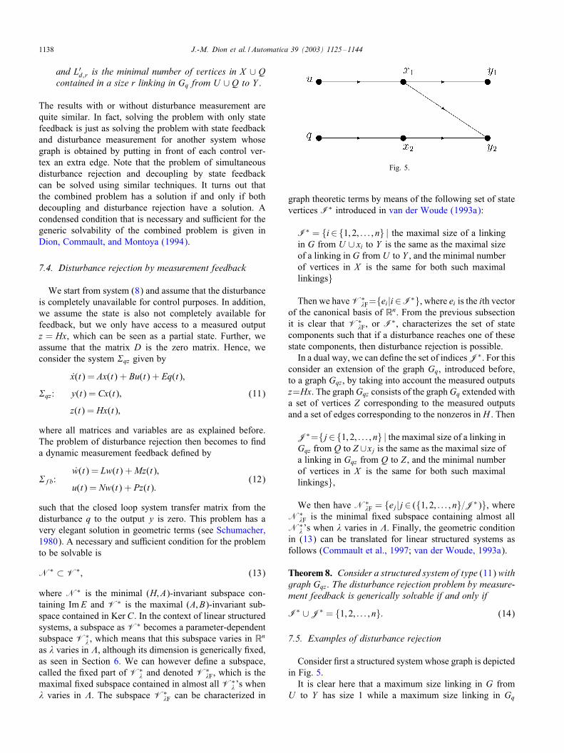
Consider 1rst a structured system whose graph is depictedin Fig. 5.It is clear here that a maximum size linking in G from
U to Y has size 1 while a maximum size linking in Gq

J.-M. Dion et al. / Automatica 39 (2003) 1125–1144 1139
Fig. 6.
from U ∪ Q to Y have size 2. Then, from Theorem 6 thedisturbance rejection problem has no solution.Consider now a system whose graph is depicted in Fig. 6.Now a maximum size linking in G from U to Y has size 1
and a maximum size linking in Gq from U ∪Q to Y has alsosize 1. The second condition of Theorem 6 is also satis1edsince L1=Ld;1=1, so that the disturbance rejection problemis solvable when the disturbance is available for controlpurposes. In contrast, the second condition of Theorem 7 isnot satis1ed, implying that disturbance rejection with statefeedback only is not possible. Roughly speaking, if we knowthe disturbance we can compensate for its action on the statex, if not the information on the disturbance comes from theknowledge of x, and it is then “too late” to compensate withthe control u for the eCect of the disturbance on the output.
8. Decentralized control
The classical problem of decentralized control can bestated as follows. We consider a system of type (5) withD = 0:
x(t) = Ax(t) + Bu(t);
y(t) = Cx(t); (15)
where x(t)∈Rn, u(t)∈Rm and y(t)∈Rp. We de1ne a feed-back pattern as a matrix< of dimension m×p consisting ofzeros and ones only. The entry<ij is one precisely when thejth output is available to control the ith input. This formula-tion allows to represent a lot of every day situations wherefor practical considerations not all outputs are allowed to beused for every input. A particular case which is often en-countered is when the matrix < is (block) diagonal. Whenapplying an output feedback F we require in this sectionthat F ∈F< where F< is de1ned as
F< = {F ∈Rm×p|Fij = 0 if <ij = 0;
for 16 i6m; 16 j6p}: (16)
The set of 1xed modes of the system (A; B; C) with respectto < is de1ned as
S< =⋂
F∈F<
>(A+ BFC); (17)
where >(·) stands for the set of eigenvalues of a matrix,counting multiplicity. This set of 1xed modes has a funda-mental importance in decentralized control since, in the case
of a (dynamic) output feedback relative to <, all the eigen-values are assignable except for the 1xed modes. The studyof 1xed modes has therefore motivated a lot of research(see for example Anderson & Clements, 1981; Corfmat &Morse, 1976a; Davison, 1973; Wang & Davison, 1973). Inthe framework of structured systems one may wonder if agiven linear structured system, being a structural version ofa system of type (15), together with a given feedback pat-tern < will give rise to generic 1xed modes. To study thisproblem 1rst we associate a graph G< to the structured sys-tem and the pattern <. For the system part this graph is ob-tained as graph G as usual. The pattern < is incorporatedby adding edges (yj; ui) to the graph G for those i; j forwhich<ij = 0. Such newly added edges are called feedbackedges. The elegant solution to the above problem is givenin Linnemann (1983) and needs the introduction of somenew botanic objects in our graph theoretic language. We callpanicle a set P composed of l mutually vertex disjoint cy-cles C1; : : : ;Cl and l+1 edges (vi; wi+1); i=0; 1; : : : ; l, suchthat viw∈Ci ; i= 0; 1; : : : ; l− 1, and the vertices v0; wl+1 donot belong to the cycles C1; : : : ;Cl. The vertex v0 is calledbegin vertex of the panicle and wi+1 the end vertex. A bunchis a subgraph that is de1ned recursively as follows. A bunchB is either a cycle, or is formed from a smaller bunch B′ towhich a panicle has been added that is vertex disjoint fromB′ apart from its begin and end vertices, which can be anytwo of vertices of B′. Finally, a bush is a set of mutuallyvertex disjoint bunches and it is called a feedback bush ifeach of its bunches contains a feedback edge. We can thenstate the next theorem (see Linnemann, 1983).
Theorem 9. Consider a structural version of system (15)with feedback pattern < as in (16) and associated graphG<. The system has no generic Bxed modes with respect to< if and only if G< contains a feedback bush which coversall the vertices of X .
For further graphic theoretic investigations on the possi-bility of control under decentralized information pattern (seeKobayashi & Yoshikawa, 1982; Kobayashi & Nakamizo,1987; Kong & Seo, 1996; Reinschke, 1991; Sezer & Siljak,1981; Trave et al., 1989).
9. Fault detection and isolation problems
In this section, we will brieRy present standard fault detec-tion and isolation (FDI) problems and some generic resultsin the context of structured systems. We will give graph the-oretic conditions under which such problems have a solutionfor almost any value of the parameters. The FDI problemhas received a considerable attention in the past 20 years,see for example Chen and Patton (1999), Frank (1996) andreferences therein. We will consider the FDI problem forlinear systems with disturbances. The problem consists ofdesigning a set of signals, called residuals, via observers for

1140 J.-M. Dion et al. / Automatica 39 (2003) 1125–1144
example, such that the transfer matrix from the disturbanceand control inputs to the residuals is zero, and the transfermatrix from the faults to the residuals has a speci1c form,e.g. diagonal or triangular. These residuals, which are insen-sitive to controls and disturbances, but sensitive to faults,will allow to detect and isolate the faults. In the frameworkof this paper we consider a structured system with faults anddisturbances (we do not consider here control inputs sinceit is well-known that their eCect can be taken into accountin the observer).
"qf�:x(t) = A�x(t) + E1�q(t) + F1�f(t);
y(t) = C�x(t) + E2�q(t) + F2�f(t);(18)
where x(t)∈Rn denotes the state of the system, q(t)∈Rd
is the disturbance, f(t)∈Rh is the fault and y(t)∈Rp themeasured output of the system. We obtain the graph Gqf
of the system "qf� from the graph G of the structured sys-tem (6) (without U ), by adding sets of vertices Q and Fcorresponding to the disturbances and faults, respectively,and edges corresponding to parameters in E1�; F1�; E2�; F2�.Consider the following observer:
˙x(t) = A�x(t) + K(�)(y(t)− C�x(t)): (19)
Note that the observer gain K(�) will depend on the param-eter �. We de1ne the residual vector as
r(t) = Q(�)(y(t)− C�x(t)); (20)
where Q(�) is a h × p matrix depending on �. Theobserver-based triangular FDI problem with disturbancesconsists in 1nding matrices K(�) and Q(�) such that
• (A� − K(�)C�) is stable,• The transfer matrix from the disturbance to the residualis zero,
• The transfer matrix from the fault to the residual is trian-gular with nonzero elements on the diagonal.
We have the following result (Commault et al., 2002).
Theorem 10. Consider a structured system of type (18)and associated graph Gqf. The observer-based triangularFDI problem with disturbances is generically solvable ifand only if
• The pair (A�; C�) is structurally observable.• k = kq + h, where k is the maximum size of a linking inGqf from Q∪F to Y , kq is the maximum size of a linkingin Gqf from Q to Y and h denotes the number of faults.
Note that this easily checkable condition is necessary andsuDcient and ensures the generic solvability of the FDI prob-lem with stability. In order to be able to detect simultaneousfaults, it is advisable to consider the observer-based diago-nal FDI problem where the transfer matrix from the fault tothe residual is required to be diagonal and nonsingular. Ithas been proved in Commault et al. (2002) that using a bank
of observers instead of a single one, the necessary and suf-1cient conditions for solving the bank of observers-baseddiagonal FDI problem with disturbances are the same asthe conditions of Theorem 10.
10. Computational aspects
10.1. Graph theoretic methods
In some parts of this paper we assumed that every ver-tex is contained in a path from U to Y in the graph G. Thisassumption is equivalent with the fact that every vertex isthe end vertex of some U -rooted path and the begin vertexof some Y -topped path. In Reinschke (1988) an algorithmis presented, using a 1nite number of boolean operations,to determine a decomposition of the graph G based on itsstrong components, (see also Schizas & Evans, 1981). Thesame techniques allow to check the solvability of the decou-pling or disturbance rejection problems (Reinschke, Jantzen,& Evans, 1991). These operations can be performed usingsymbolic calculus as in Franksen, Falster, and Evans (1979).
10.2. Flow theoretic methods
A lot of the results appearing in the previous sections areexpressed in terms of input–output linkings in the graph Gassociated with a structured system. In the determination ofthe rank of the transfer matrix we look for the maximumsize of a linking in G between U and Y , while in the deter-mination of the structure at in1nity we search for minimalnumber of vertices in X contained in linkings in G fromU to Y of increasing sizes. It turns out that these problemscan be transformed into standard Row problems for instance.For this we need 1rst to transform the graph G into a Rownetwork as follows:
• Create a dummy vertex, called a source, and add edgesfrom this vertex to all input vertices in U .
• Create a dummy vertex, called sink, and add edges fromall output vertices in Y to this vertex.
• Split each state vertex xi into two vertices xi1 and xi2,and create an edge from xi1 to xi2, i.e. an edge (xi1; xi2).Further, transform each edge of the form (xi; xj); (ui; xj)and (xi; yj) of the original graph into an edge of the form(xi2; xj1); (ui; xj1) and (xi2; yj), respectively, in the Rownetwork. Leave edges of the form (ui; yj) as they are.
• Give a capacity 1 to each edge of the Row network. Assigna cost 1 to each of the newly introduced edges (xi1; xi2)and cost 0 to all the other edges.
The maximal size linking problem in the original graph isthen equivalent to the maximal Row problem in the Rownetwork, and the minimal number of vertices in X con-tained in a size k linking in G from U to Y is equal to theminimal costs of a Row of strength k in the Row network.
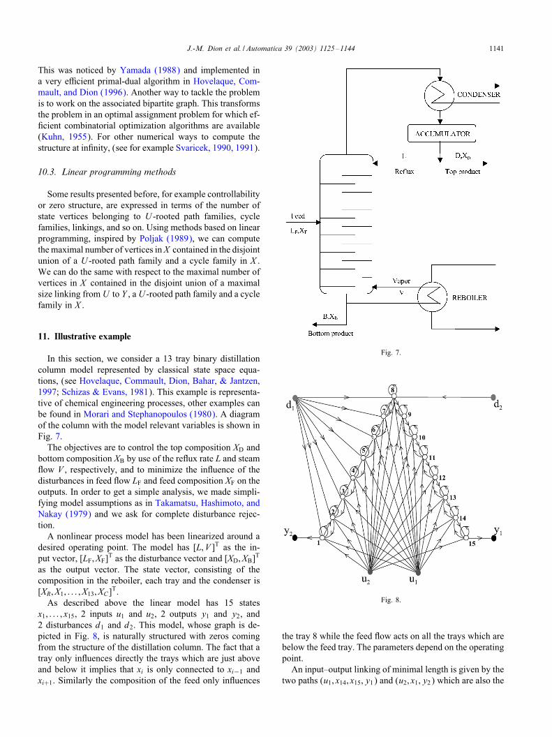
J.-M. Dion et al. / Automatica 39 (2003) 1125–1144 1141
This was noticed by Yamada (1988) and implemented ina very eDcient primal-dual algorithm in Hovelaque, Com-mault, and Dion (1996). Another way to tackle the problemis to work on the associated bipartite graph. This transformsthe problem in an optimal assignment problem for which ef-1cient combinatorial optimization algorithms are available(Kuhn, 1955). For other numerical ways to compute thestructure at in1nity, (see for example Svaricek, 1990, 1991).
10.3. Linear programming methods
Some results presented before, for example controllabilityor zero structure, are expressed in terms of the number ofstate vertices belonging to U -rooted path families, cyclefamilies, linkings, and so on. Using methods based on linearprogramming, inspired by Poljak (1989), we can computethe maximal number of vertices in X contained in the disjointunion of a U -rooted path family and a cycle family in X .We can do the same with respect to the maximal number ofvertices in X contained in the disjoint union of a maximalsize linking fromU to Y , aU -rooted path family and a cyclefamily in X .
11. Illustrative example
In this section, we consider a 13 tray binary distillationcolumn model represented by classical state space equa-tions, (see Hovelaque, Commault, Dion, Bahar, & Jantzen,1997; Schizas & Evans, 1981). This example is representa-tive of chemical engineering processes, other examples canbe found in Morari and Stephanopoulos (1980). A diagramof the column with the model relevant variables is shown inFig. 7.The objectives are to control the top composition XD and
bottom composition XB by use of the reRux rate L and steamRow V , respectively, and to minimize the inRuence of thedisturbances in feed Row LF and feed composition XF on theoutputs. In order to get a simple analysis, we made simpli-fying model assumptions as in Takamatsu, Hashimoto, andNakay (1979) and we ask for complete disturbance rejec-tion.A nonlinear process model has been linearized around a
desired operating point. The model has [L; V ]T as the in-put vector, [LF; XF]T as the disturbance vector and [XD; XB]T
as the output vector. The state vector, consisting of thecomposition in the reboiler, each tray and the condenser is[XR; X1; : : : ; X13; XC]T.As described above the linear model has 15 states
x1; : : : ; x15, 2 inputs u1 and u2, 2 outputs y1 and y2, and2 disturbances d1 and d2. This model, whose graph is de-picted in Fig. 8, is naturally structured with zeros comingfrom the structure of the distillation column. The fact that atray only inRuences directly the trays which are just aboveand below it implies that xi is only connected to xi−1 andxi+1. Similarly the composition of the feed only inRuences
Fig. 7.
Fig. 8.
the tray 8 while the feed Row acts on all the trays which arebelow the feed tray. The parameters depend on the operatingpoint.An input–output linking of minimal length is given by the
two paths (u1; x14; x15; y1) and (u2; x1; y2) which are also the
1142 J.-M. Dion et al. / Automatica 39 (2003) 1125–1144
shortest paths from control inputs to y1 and y2, respectively.Then the generic in1nite structure is given by (2; 1), seeTheorem 2, and the decoupling condition of Theorem 5 issatis1ed. The distillation column is generically decouplableby a state feedback control law of the form u(t) = Fx(t) +Gv(t), where F and G depend on the parameters. Such afeedback is given in Hovelaque et al. (1997).Consider now the disturbance rejection problem when
the disturbance is available for measurement. Since theabove-mentioned linking is also a linking of minimal lengthfrom control inputs plus disturbances to the outputs, thecondition of Theorem 6 is also satis1ed and state feed-back disturbance rejection with disturbance measurement isgenerically solvable. It can be shown using Theorem 7 thatwhen the disturbances are not available for measurementthe disturbance d1 cannot be rejected.
12. Concluding remarks
In this paper, we have dealt with generic properties oflinear systems. We have focused our interest on linear struc-tured systems which arise naturally when modelling real sys-tems. We have shown that a lot of structural properties andgeneric solvability conditions of classical control problemscan be checked easily on the graph associated to a linearsystem. It appears that strong generic results can be obtainedfrom poor information on the system. Similar graph theo-retic ideas have been used also for analysing other classesof systems. We can mention for example extensions to timedelay systems (Sename, Hovelaque, Commault, & Dion,2001), implicit systems (Pantelides, 1988; van der Woude,1995) or nonlinear systems (Kasinski & Levine, 1984). In-teresting similar ideas have also been applied to bond graphmodels which do not require the parameters independency(Bertrand, Sueur, & Dauphin-Tanguy, 1997; Gawthrop &Smith, 1996), as it is implicitly assumed in the frameworkof this paper.Some interesting questions remain open in the frame-
work of this paper. For example, the characterization ofthe generic controllability indices (Poljak, 1992; Reinschke,1984) of a linear structured system. We gave some stabilityresults, for instance in the FDI problems, but in general to getstabilizability results in our framework, more information onthe system is required than just the zero/nonzero structurealone (JeCries, 1974; JeCries, Klee, & van der Driessche,1977).The major part of this paper is based on structured state
space models whose analysis is fairly simple. Starting fromother models presented in Section 2, the same kind of re-sults as those of this paper could be looked for. Much workremains also to be done concerning the modelling aspects,in particular it would be of strong interest to get “minimal”parametrizations in terms of independent parameters.
References
Aling, H., & Schumacher, J. M. (1984). A nine-fold canonicaldecomposition for linear systems. International Journal of Control,39, 779–805.
Anderson, B. D. O., & Clements, D. J. (1981). Algebraic characterizationof 1xed modes in decentralized control systems. Automatica, 17, 703–712.
Anderson, B. D. O., & Hong, H. M. (1982). Structural controllabilityand matrix nets. International Journal of Control, 17, 397–416.
Basile, G., & Marro, G. (1969). Controlled and conditioned invariantsubspaces in linear system theory. Journal of Optimization Theoryand Applications, 3(5), 306–315.
Bertrand, J., Sueur, C., & Dauphin-Tanguy, G. (1997). Bond graph formodeling and control: Structural analysis tools for the design of input–output decoupling state feedbacks. In International conference on bondgraph modeling and simulation.
Chen, J., & Patton, R. J. (1999). Robust model-based fault diagnosis fordynamic systems. Dordrecht: Kluwer Academic Publishers.
Commault, C., Dion, J. M., & Belmehdi, A. (1987). Structured systemswithin the transfer matrix approach: Application to decoupling.Systems & Control Letters, 9, 335–339.
Commault, C., Dion, J. M., & BenahcJene, M. (1993). Output feedbackdisturbance decoupling—graph interpretation for structured systems.Automatica, 29, 1463–1472.
Commault, C., Dion, J. M., & Hovelaque, V. (1997). A geometricapproach for structured systems: Application to the disturbancedecoupling problem. Automatica, 33, 403–409.
Commault, C., Dion, J. M., & Perez, A. (1991). Disturbance rejectionfor structured systems. IEEE Transactions on Automatic Control,AC-36, 884–887.
Commault, C., Dion, J. M., Sename, O., & Motyeian, R. (2002).Observer-based fault diagnosis for structured systems. IEEETransactions on Automatic Control, AC-47, 2074–2079.
Corfmat, J. P., & Morse, A. S. (1976a). Decentralized control of linearmultivariable systems. Automatica, 12, 479–495.
Corfmat, J. P., & Morse, A. S. (1976b). Structurally controllable andstructurally canonical systems. IEEE Transactions on AutomaticControl, AC-21, 129–131.
Davison, E. J. (1973). Connectability and structural controllability ofcomposite systems. IEEE Transactions on Automatic Control, AC-18,24–32.
Davison, E. J., & Wang, S. H. (1973). Properties of linear time-invariantmultivariable systems subject to arbitrary output and state feedback.IEEE Transactions on Automatic Control, AC-18, 24–32.
Davison, E. J., & Wang, S. H. (1974). Properties and calculationof transmission zeros of linear multivariable time-invariant systems.Automatica, 10, 643–658.
Descusse, J., & Dion, J. M. (1982). On the structure at in1nity oflinear square decouplable systems. IEEE Transactions on AutomaticControl, AC-27, 971–974.
Dion, J. M., & Commault, C. (1982). Smith-Mcmillan factorisations atin1nity of rational matrix functions and their control interpretation.Systems & Control Letters, 1, 312–320.
Dion, J. M., & Commault, C. (1993). Feedback decoupling of structuredsystems. IEEE Transactions on Automatic Control, AC-38, 1132–1135.
Dion, J. M., Commault, C., & Montoya, J. (1994). Simultaneousdecoupling and disturbance rejection—a structural approach.International Journal of Control, 59, 1325–1344.
Dion, J. M., Commault, C., & van der Woude, J. (2001). Genericproperties and control of linear structured systems. In First IFACsymposium on system structure and control, Prague.
Frank, P. M. (1996). Analytical and qualitative model-based faultdiagnosis—a survey and some new results. European Journal ofControl, 2, 6–28.

J.-M. Dion et al. / Automatica 39 (2003) 1125–1144 1143
Franksen, O. I., Falster, P., & Evans, F. J. (1979). Qualitative aspectsof large scale systems. Berlin: Springer.
Gawthrop, P., & Smith, L. (1996). Metamodelling: Bond graphs anddynamic systems. Englewood CliCs, NJ: Prentice-Hall.
Glover, K., & Silverman, L. M. (1976). Characterization of structuralcontrollability. IEEE Transactions on Automatic Control, AC-21,534–537.
Hayakawa, Y., & Silijak, D. D. (1988). On almost invariant subspacesof structured systems and decentralized control. IEEE Transactionson Automatic Control, AC-33, 931–939.
Hosoe, S. (1980). Determination of generic dimensions of controllablesubspaces and its application. IEEE Transactions on AutomaticControl, AC-25, 1192–1196.
Hovelaque, V., Commault, C., & Dion, J. M. (1996). Analysis of linearstructured systems using a primal-dual algorithm. Systems & ControlLetters, 27, 73–85.
Hovelaque, V., Commault, C., & Dion, J. M. (1999). Zeros of structuredlinear systems. Automatica, 35, 1683–1688.
Hovelaque, V., Commault, C., Dion, J. M., Bahar, M., & Jantzen, J.(1997). Graph modelling approach, application to a distillation column.Studies in Informatics and Control, 6, 87–96.
Jantzen, J. (1994). Digraph approach to multivariable control. Technicalreport, Technical University of Denmark, Lyngby.
JeCries, C. (1974). Qualitative stability and digraphs in ecosystems.Ecology, 55, 1415–1419.
JeCries, C., Klee, V., & van den Driessche, P. (1977). When is a matrixsign stable. Canadian Journal of Mathematics, XXIX, 315–326.
Kailath, T. (1980). Linear systems. Englewood CliCs, NJ: Prentice-Hall.Kasinski, A., & Levine, J. (1984). A fast graph theoretic algorithm for the
feedback decoupling problem of nonlinear systems. In Mathematicaltheory of networks and systems, Lectures notes in control andinformation sciences, Vol. 58, Prague (pp. 550–562). Berlin: Springer.
Kobayashi, N., & Nakamizo, T. (1987). A disturbance rejection problem instructural aspects. Transactions of Society of Instrument and ControlEngineers, 23, 48–54 (in Japanese).
Kobayashi, H., & Yoshikawa, T. (1982). Graph–theoretic approach tocontrollability and localizability of decentralized control systems. IEEETransactions on Automatic Control, AC-27, 1096–1107.
Kong, J., & Seo, J. H. (1996). Graph-theoretic characterization of 1xedmodes in frequency domain. Automatica, 32, 1057–1060.
Kuhn, H. W. (1955). The hungarian method for the assignment problem.Naval Research Logistics Quarterly, 2, 83–97.
Lin, C. T. (1974). Structural controllability. IEEE Transactions onAutomatic Control, AC-19, 201–208.
Linnemann, A. (1981). Decoupling of structured systems. Systems &Control Letters, 1, 79–86.
Linnemann, A. (1983). Fixed modes in parametrized systems.International Journal of Control, 38, 319–335.
Morari, M., & Stephanopoulos, G. (1980). Studies in the synthesis ofcontrol structures for chemical processes, Part II: Structural aspectsand the synthesis of alternative feasible control schemes. A.I.Ch.E.Journal, 26, 232–246.
Murota, K. (2000). Matrices and matroids for systems analysis. InAlgorithms and combinatorics, Vol. 20. Berlin: Springer.
Murota, K., & van der Woude, J. W. (1991). Structure at in1nity ofstructured descriptor systems and its applications. SIAM Journal onControl and Optimization, 29, 878–894.
Ohta, Y., & Kodama, S. (1985). Structural invertibility of transferfunctions. IEEE Transactions on Automatic Control, AC-30, 818–819.
Pantelides, C. C. (1988). The consistent initialization of diCerential-algebraic systems. SIAM Journal on Statistical Computation, 9, 213–231.
Poljak, S. (1989). Maximum rank of powers of a matrix of a given pattern.Proceedings of the American Mathematical Society, 4, 1137–1144.
Poljak, S. (1992). On the gap between the structural controllabilityof time-varying and time-invariant systems. IEEE Transactions onAutomatic Control, AC-37, 1961–1965.
Reinschke, K. J. (1984). Graph-theoretic characterisation of structuralproperties by means of paths and cycle families. In IFAC worldcongress, Budapest.
Reinschke, K. J. (1988). Multivariable control, a graph-theoreticapproach. Berlin: Springer.
Reinschke, K. J., Jantzen, J., & Evans, F. J. (1991). CAD techniques fora structural approach to non interaction and disturbance rejection. InIFAC symposium on design methods of control systems, Zurich (pp.825–830).
Rosenbrock, H. H. (1970). State-space and multivariable theory. NewYork: Wiley.
Schizas, C., & Evans, F. J. (1981). A graph theoretic approach tomultivariable control system design. Automatica, 17, 371–377.
Schumacher, J. M. (1980). Compensator synthesis using (C,A,B) pairs.IEEE Transactions on Automatic Control, AC-25, 1133–1138.
Sename, O., Hovelaque, V., Commault, C., & Dion, J. M. (2001).Structured time delay systems: A graph approach. InternationalJournal of Control, 74, 373–386.
Sezer, M. E., & Siljak, D. D. (1981). Structurally 1xed modes. Systems& Control Letters, 1, 60–64.
Shields, R. W., & Pearson, J. B. (1976). Structural controllability ofmulti-input linear systems. IEEE Transactions on Automatic Control,AC-21, 203–212.
Sote, W. (1980). Eine graphische methode zur ermittlung der nullstellenin mehrgr[ossen-systemen. Reglungstechnik, 28, 346–348.
Suda, N., Wan, B., & Ueno, I. (1989). The orders of in1nite zeros ofstructured systems. Transactions of the Society of Instrument ControlEngineers, 25, 346–348.
Svaricek, F. (1986). Graphentheoretische ermittlung der anzahlvon strukturellen und streng strukturellen invarianten nullstellen.Automatisierungstechnik, 34, 488–497.
Svaricek, F. (1990). An improved graph-theoretic algorithm for computingthe structure at in1nity of linear systems. In IEEE CDC conference,Hawaii.
Svaricek, F. (1991). Computation of the generic structure at in1nity oflinear systems: A Toeplitz-matrix approach. In 13th IMACS worldcongress on computation and applied mathematics, Dublin (pp. 1130–1132).
Takamatsu, T., Hashimoto, I., & Nakay, Y. (1979). A geometric approachto multivariable system design of a distillation column. Automatica,15, 387–402.
Trave, L., Titli, A., & Tarras, A.M. (1989). Large scale systems:Decentralization, structure constraints and Bxed modes. Berlin:Springer.
van der Woude, J. W. (1991a). A graph theoretic characterization for therank of the transfer matrix of a structured system. Mathematics ofControl, Signals and Systems, 4, 33–40.
van der Woude, J. W. (1991b). On the structure at in1nity of a structuredsystem. Linear Algebra and its Applications, 148, 145–169.
van der Woude, J. W. (1993a). Disturbance decoupling by measurementfeedback for structured systems: A graph theoretic approach. InProccedings of second European control conference ECC’93,Groningen (pp. 1132–1137).
van der Woude, J. W. (1993b). Disturbance decoupling by measurementfeedback for structured transfer matrix systems. Automatica, 32, 357–364.
van der Woude, J. W. (1995). The generic dimension of a minimalrealization of an AR-system. Mathematics of Control, Signals andSystems, 8, 50–64.
van der Woude, J. W. (1997). Graph theoretic conditions for structuraldisturbance decoupling with pole placement. In European controlconference ECC’97, Brussels.
van der Woude, J. W. (2000). The generic number of invariant zeros of astructured linear system. SIAM Journal on Control and Optimization,38, 1–21.

1144 J.-M. Dion et al. / Automatica 39 (2003) 1125–1144
van der Woude, J. W., Commault, C., & Dion, J. M. (2000). Invariants forlinear structured systems. Technical report, Laboratoire d’Automatiquede Grenoble, France.
van der Woude, J. W., & Murota, K. (1995). Disturbance decouplingwith pole placement for structured systems; a graph theoreticapproach. SIAM Journal on Matrix Analysis and Applications, 16(3),922–942.
Wang, S. H., & Davison, E. J. (1973). On the stabilisation of decentralizedcontrol systems. IEEE Transactions on Automatic Control, AC-18,473–478.
Wonham, W. M. (1985). Linear multivariable control: A geometricapproach. Berlin: Springer.
Yamada, T. (1988). A network Row algorithm to 1nd an elementary i/omatching. Networks, 18, 105–109.
Jean-Michel Dion was born in 1950 in LaTronche, France. He received the Ph.D. de-gree from the National Polytechnic Insti-tute of Grenoble (INPG), France in 1977.From 1977 to 1979 he was a visiting pro-fessor at the National Polytechnic Instituteof Mexico city. Since 1979, he has beena researcher at the French National Centerfor Scienti1c Research (CNRS). He was di-rector of the Laboratoire d’Automatique deGrenoble and vice president of the National-Polytechnic Institute of Grenoble. He is cur-
rently director of a federative research institute (ELESA) in the 1eldsof microelectronics, signal processing, electrical engineering, control andtelecommunications and is director of the department of Physics and En-gineering Sciences at the French Ministry of Research. His main researchinterests are in the 1elds of linear system theory, adaptive control, robustcontrol, and time delay systems with application to electromechanicalsystems. Jean-Michel Dion was associate editor of Automatica. He waschairman of the IFAC technical committee Linear Systems, he is nowmember of the IFAC Council.
Christian Commault was born in 1950 inLe Gouray, France. He received the En-gineer degree, the Doctor-Engineer degreeand the ‘Docteur d’ Etat’ degree from theInstitut National Polytechnique de Greno-ble in 1973, 1978 and 1983, respectively.He taught 2 years in the Dakar Instituteof Technology (S]en]egal). He was a visit-ing researcher in the department of mathe-matics at the University of Groningen (TheNetherlands) during 1 year. From 1986 to1988 he worked in the Research Centre of
Renault, Rueil-Malmaison. He is currently a professor at the Ecole Na-tionale Sup]erieure d’ Ing]enieurs Electriciens de Grenoble (ENSIEG). Heteaches basic control systems, multivariable systems, operation researchand performance evaluation.He is a researcher of the Laboratoire d’Automatique de Grenoble (LAG).His main research interests are in performance evaluation of productionsystems and in linear multivariable systems (mainly in structured systemsboth for control and diagnosis).
Jacob W. van der Woude obtained the M.S.degree in mathematics from the Rijksuni-versiteit Groningen in 1981. In 1982, hewas involved as a researcher in a project ofthe N.V. Nederlandse Gasunie in Gronin-gen. From 1983 till 1987 he worked in thesystem theory group of the Department ofMathematics and Computing Science of theEindhoven University of Technology wherehe obtained the doctoral degree in 1987. In1988 and 1989 he was attached as a re-search fellow at the Center for Mathematics
and Computer Science in Amsterdam. Since 1990 he is working in thesystem theory group of the Faculty of Information Technology and Sys-tems of the Delft University of Technology. His current research inter-ests include system and control theory, discrete event systems, switchingnetworks and applied graph theory.