Embed Size (px)
DESCRIPTION
survivalpart8
Citation preview
1
Survival Models in SAS Part 8: PROC PHREG – Part 3
June 18, 2008
Charlie Hallahan
2
Chapter 5: Estimating Cox Regression Models with PROC PHREG
These talks are based on the book “Survival Analysis Using the SAS System: A Practical Guide” (1995) by Paul Allison.
The book is part of the SAS Books-by-Users series and can be found at http://www.sas.com/apps/pubscat/bookdetails.jsp?catid=1&pc=55233
3
Chapter 5: Estimating Cox Regression Models with PROC PHREG
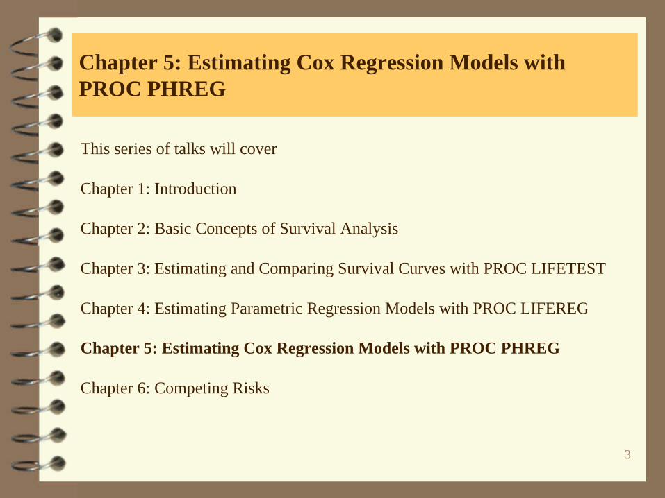
This series of talks will cover
Chapter 1: Introduction
Chapter 2: Basic Concepts of Survival Analysis
Chapter 3: Estimating and Comparing Survival Curves with PROC LIFETEST
Chapter 4: Estimating Parametric Regression Models with PROC LIFEREG
Chapter 5: Estimating Cox Regression Models with PROC PHREG
Chapter 6: Competing Risks
4
Chapter 5: Estimating Cox Regression Models with PROC PHREG
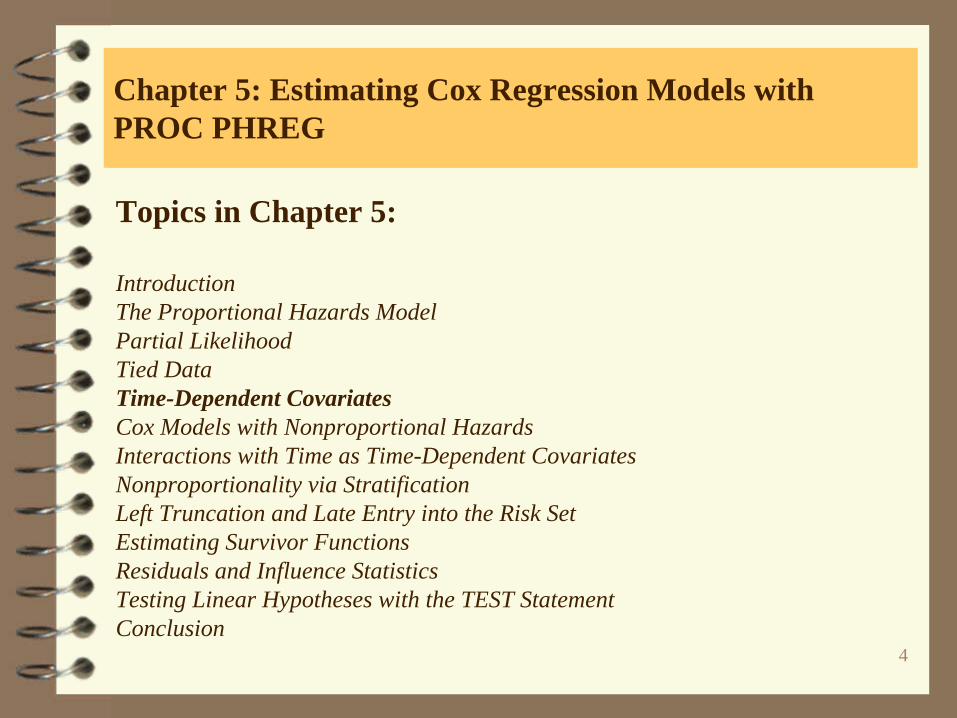
Topics in Chapter 5:
IntroductionThe Proportional Hazards ModelPartial LikelihoodTied DataTime-Dependent CovariatesCox Models with Nonproportional HazardsInteractions with Time as Time-Dependent CovariatesNonproportionality via StratificationLeft Truncation and Late Entry into the Risk SetEstimating Survivor FunctionsResiduals and Influence StatisticsTesting Linear Hypotheses with the TEST StatementConclusion
5
Chapter 5: Estimating Cox Regression Models with PROC PHREG: Time-Dependent Covariates
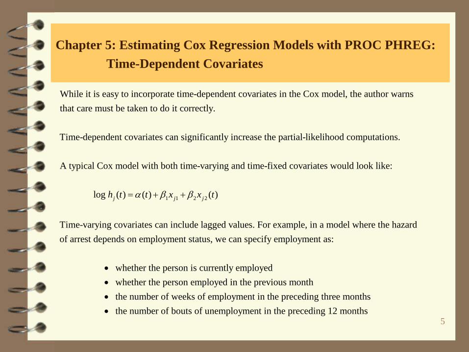
While it is easy to incorporate time-dependent covariates in the Cox model, the author warnsthat care must be taken to do it correctly.
Time-dependent covariates can significantly increase the partial-
1 1 2 2
likelihood computations.
A typical Cox model with both time-varying and time-fixed covariates would look like:
log ( ) ( ) ( )
Time-varying covariates can include lagged value
j j jh t t x x tα β β= + +
s. For example, in a model where the hazardof arrest depends on employment status, we can specify employment as:
whether the person is currently employed whethe
•• r the person employed in the previous month
the number of weeks of employment in the preceding three months the number of bouts of unemployment in the preceding
•• 12 months
6
Chapter 5: Estimating Cox Regression Models with PROC PHREG: Time-Dependent Covariates: Heart Transplant Example
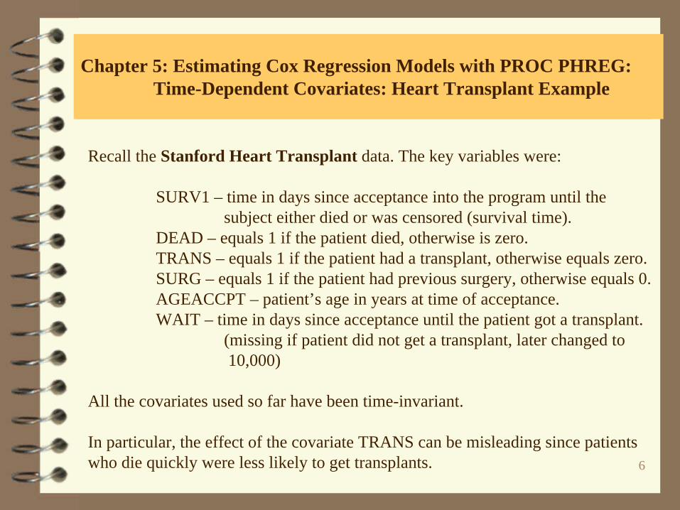
Recall the Stanford Heart Transplant data. The key variables were:
SURV1 – time in days since acceptance into the program until the subject either died or was censored (survival time).
DEAD – equals 1 if the patient died, otherwise is zero.TRANS – equals 1 if the patient had a transplant, otherwise equals zero.SURG – equals 1 if the patient had previous surgery, otherwise equals 0.AGEACCPT – patient’s age in years at time of acceptance.WAIT – time in days since acceptance until the patient got a transplant.
(missing if patient did not get a transplant, later changed to 10,000)
All the covariates used so far have been time-invariant.
In particular, the effect of the covariate TRANS can be misleading since patients who die quickly were less likely to get transplants.
7
Chapter 5: Estimating Cox Regression Models with PROC PHREG: Time-Dependent Covariates: Heart Transplant Example
The author introduces a new time-varying covariate called PLANT which is equal to 1 if the patient already had a transplant at day t, otherwise PLANT is equal to 0.
PHREG provides a number of the DATA step operators and functions that are needed to create time-varying covariates.
In this example, an IF statement is used in PHREG to create PLANT.
The behavior of the IF statement in PHREG is radically different than its behavior in the DATA step.
This will become much clearer in the next section when it is shown how the partial likelihood function is created in the presence of an IF statement.
8
Chapter 5: Estimating Cox Regression Models with PROC PHREG: Time-Dependent Covariates: Heart Transplant Example
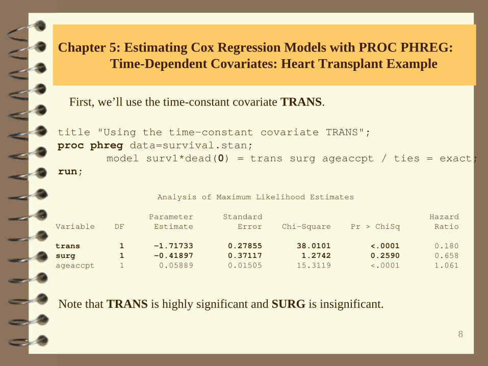
title "Using the time-constant covariate TRANS";proc phreg data=survival.stan;
model surv1*dead(0) = trans surg ageaccpt / ties = exact;run;
Analysis of Maximum Likelihood Estimates
Parameter Standard HazardVariable DF Estimate Error Chi-Square Pr > ChiSq Ratio
trans 1 -1.71733 0.27855 38.0101 <.0001 0.180surg 1 -0.41897 0.37117 1.2742 0.2590 0.658ageaccpt 1 0.05889 0.01505 15.3119 <.0001 1.061
First, we’ll use the time-constant covariate TRANS.
Note that TRANS is highly significant and SURG is insignificant.
9
Chapter 5: Estimating Cox Regression Models with PROC PHREG: Time-Dependent Covariates: Heart Transplant Example
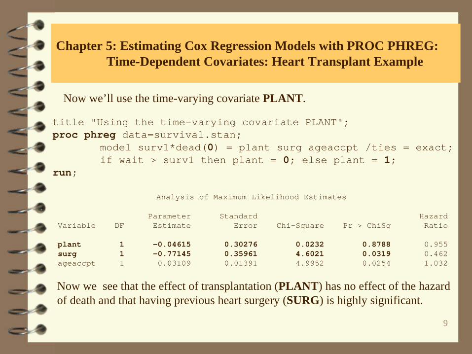
Now we’ll use the time-varying covariate PLANT.
title "Using the time-varying covariate PLANT";proc phreg data=survival.stan;
model surv1*dead(0) = plant surg ageaccpt /ties = exact;if wait > surv1 then plant = 0; else plant = 1;
run;
Analysis of Maximum Likelihood Estimates
Parameter Standard HazardVariable DF Estimate Error Chi-Square Pr > ChiSq Ratio
plant 1 -0.04615 0.30276 0.0232 0.8788 0.955surg 1 -0.77145 0.35961 4.6021 0.0319 0.462ageaccpt 1 0.03109 0.01391 4.9952 0.0254 1.032
Now we see that the effect of transplantation (PLANT) has no effect of the hazard of death and that having previous heart surgery (SURG) is highly significant.
10
Chapter 5: Estimating Cox Regression Models with PROC PHREG: Time-Dependent Covariates: Heart Transplant Example
If we put this same IF statement in a DATA step, we would see that the new variable PLANT would be identical to TRANS. The value of SURV1 and WAIT used for each comparison would always be for the current observation.
However, in PHREG (which needs to calculate the partial likelihood function), the value of SURV1 would be for a given observation and the values for WAIT would range over all observations in the current risk set.
This will become clearer in the next section.
11
Chapter 5: Estimating Cox Regression Models with PROC PHREG: Time-Dependent Covariates: Construction of the Partial
Likelihood with Time-dependent Covariates
1 1
1
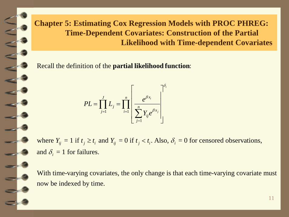
Recall the definition of the :
where = 1 if and = 0 if . Also, = 0 for censored
i
i
j
xJ n
j nxj i
ijj
ij j i ij j i i
ePL LY e
Y t t Y t t
δ
β
β
δ
= =
=
⎡ ⎤⎢ ⎥⎢ ⎥= =⎢ ⎥⎢ ⎥⎣ ⎦
≥ <
∏ ∏∑
partial likelihood function
observations,
and = 1 for failures.
With time-varying covariates, the only change is that each time-varying covariate mustnow be indexed by time.
iδ
12
Chapter 5: Estimating Cox Regression Models with PROC PHREG: Time-Dependent Covariates: Construction of the Partial
Likelihood with Time-dependent Covariates
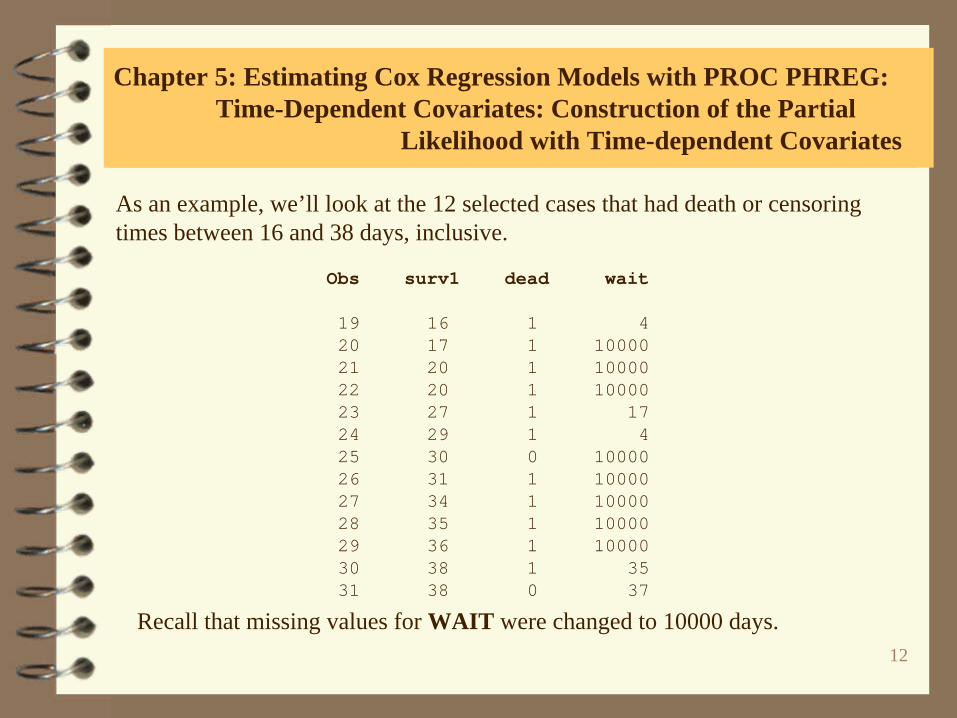
As an example, we’ll look at the 12 selected cases that had death or censoring times between 16 and 38 days, inclusive.
Obs surv1 dead wait
19 16 1 420 17 1 1000021 20 1 1000022 20 1 1000023 27 1 1724 29 1 425 30 0 1000026 31 1 1000027 34 1 1000028 35 1 1000029 36 1 1000030 38 1 3531 38 0 37
Recall that missing values for WAIT were changed to 10000 days.
13
Chapter 5: Estimating Cox Regression Models with PROC PHREG: Time-Dependent Covariates: Construction of the Partial
Likelihood with Time-dependent Covariates
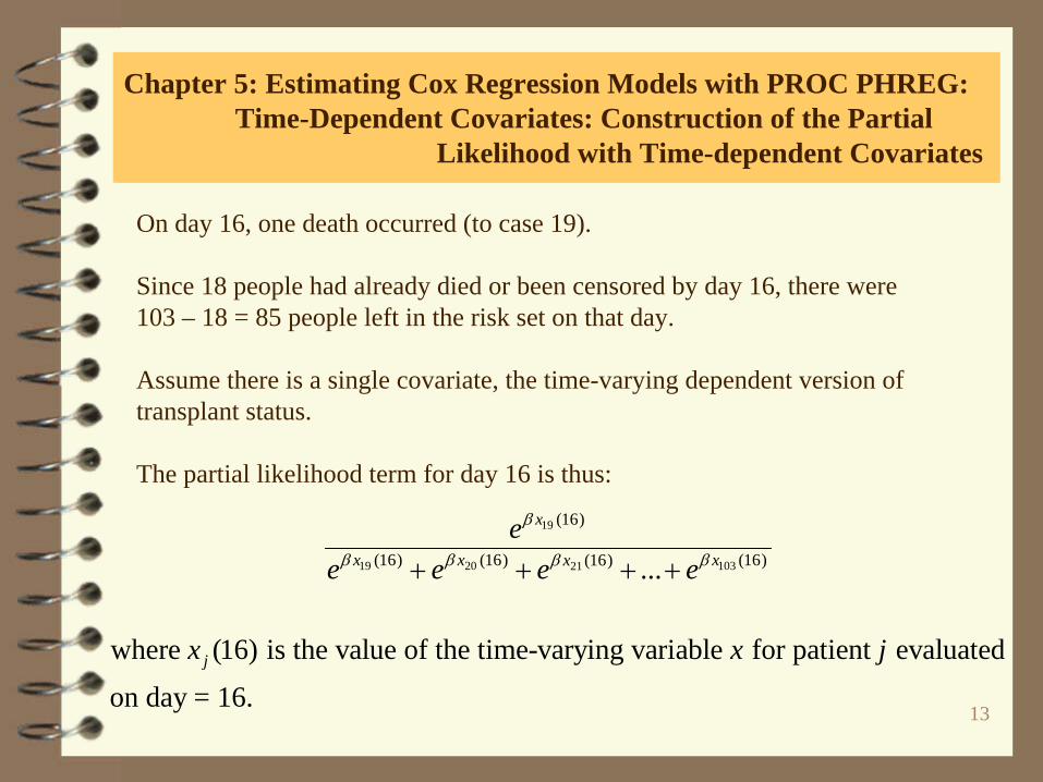
On day 16, one death occurred (to case 19).
Since 18 people had already died or been censored by day 16, there were 103 – 18 = 85 people left in the risk set on that day.
Assume there is a single covariate, the time-varying dependent version of transplant status.
The partial likelihood term for day 16 is thus:
19
19 20 10321
(16)
(16) (16) (16)(16) ...
where (16) is the value of the time-varying variable for patient evaluated
on day = 16.
x
x x xx
j
ee e e e
x x j
β
β β ββ+ + + +
14
Chapter 5: Estimating Cox Regression Models with PROC PHREG: Time-Dependent Covariates: Construction of the Partial
Likelihood with Time-dependent Covariates
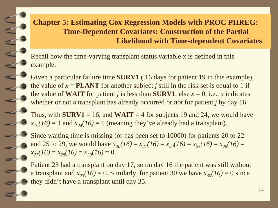
Recall how the time-varying transplant status variable x is defined in this example.
Given a particular failure time SURV1 ( 16 days for patient 19 in this example), the value of x = PLANT for another subject j still in the risk set is equal to 1 if the value of WAIT for patient j is less than SURV1, else x = 0, i.e., x indicates whether or not a transplant has already occurred or not for patient j by day 16.
Thus, with SURV1 = 16, and WAIT = 4 for subjects 19 and 24, we would have x19 (16) = 1 and x24 (16) = 1 (meaning they’ve already had a transplant).
Since waiting time is missing (or has been set to 10000) for patients 20 to 22 and 25 to 29, we would have x20 (16) = x21 (16) = x22 (16) = x25 (16) = x26 (16) = x27 (16) = x28 (16) = x29 (16) = 0.
Patient 23 had a transplant on day 17, so on day 16 the patient was still without a transplant and x23 (16) = 0. Similarly, for patient 30 we have x30 (16) = 0 since they didn’t have a transplant until day 35.
15
Chapter 5: Estimating Cox Regression Models with PROC PHREG: Time-Dependent Covariates: Construction of the Partial
Likelihood with Time-dependent Covariates
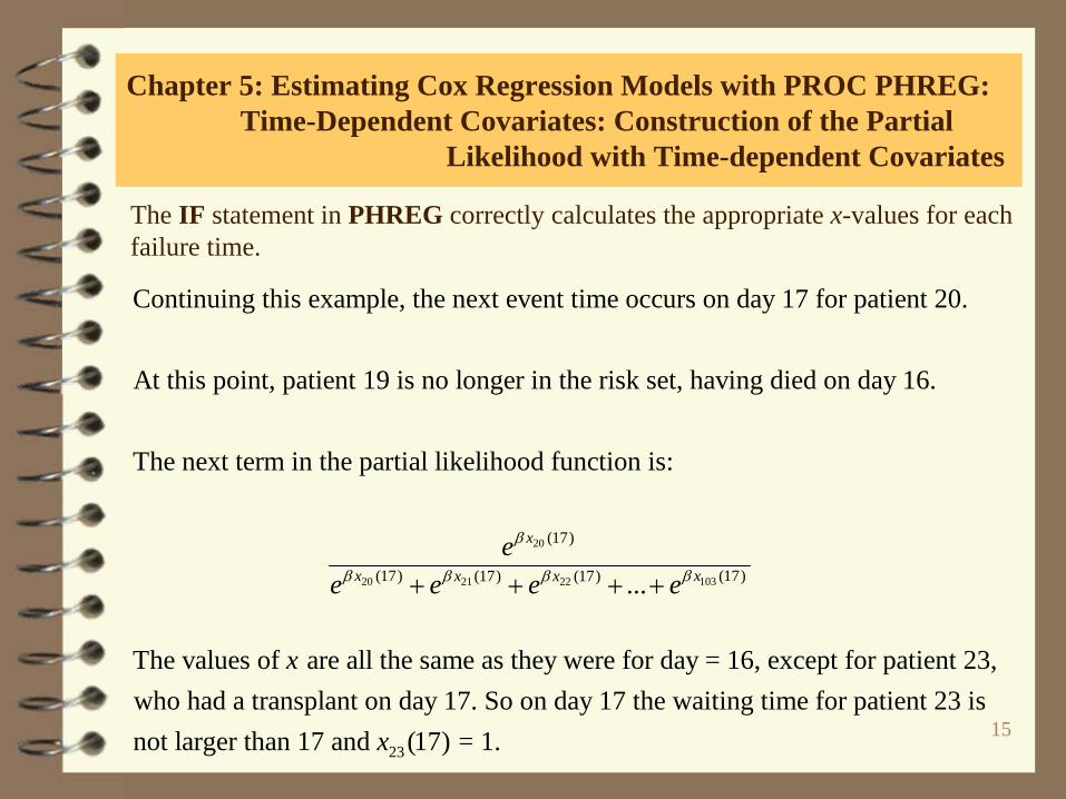
The IF statement in PHREG correctly calculates the appropriate x-values for each failure time.
Continuing this example, the next event time occurs on day 17 for patient 20.
At this point, patient 19 is no longer in the risk set, having died on day 16.
The next term in the partial likelihood func
20
20 10321 22
(17)
(17) (17)(17) (17)
tion is:
...
The values of are all the same as they were for day = 16, except for patient 23,who had a transplant on day 1
x
x xx xe
e e e e
x
β
β ββ β+ + + +
23
7. So on day 17 the waiting time for patient 23 is not larger than 17 and (17) = 1. x
16
Chapter 5: Estimating Cox Regression Models with PROC PHREG: Time-Dependent Covariates: Construction of the Partial
Likelihood with Time-dependent Covariates
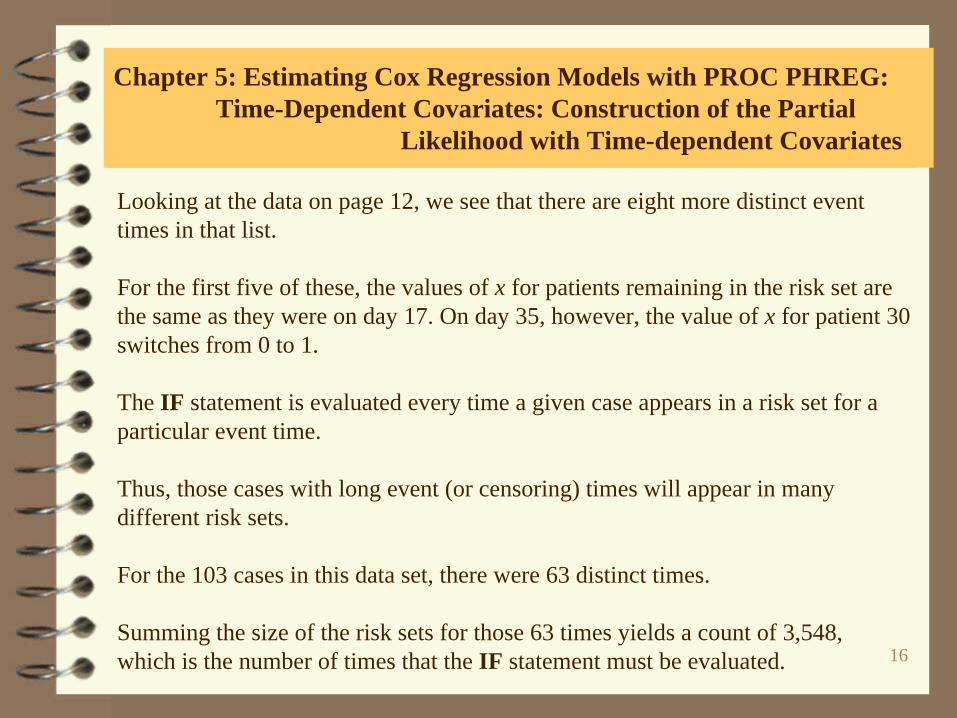
Looking at the data on page 12, we see that there are eight more distinct event times in that list.
For the first five of these, the values of x for patients remaining in the risk set are the same as they were on day 17. On day 35, however, the value of x for patient 30 switches from 0 to 1.
The IF statement is evaluated every time a given case appears in a risk set for a particular event time.
Thus, those cases with long event (or censoring) times will appear in many different risk sets.
For the 103 cases in this data set, there were 63 distinct times.
Summing the size of the risk sets for those 63 times yields a count of 3,548, which is the number of times that the IF statement must be evaluated.
17
Chapter 5: Estimating Cox Regression Models with PROC PHREG: Time-Dependent Covariates: Construction of the Partial
Likelihood with Time-dependent Covariates
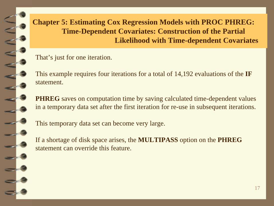
That’s just for one iteration.
This example requires four iterations for a total of 14,192 evaluations of the IF statement.
PHREG saves on computation time by saving calculated time-dependent values in a temporary data set after the first iteration for re-use in subsequent iterations.
This temporary data set can become very large.
If a shortage of disk space arises, the MULTIPASS option on the PHREG statement can override this feature.
18
Chapter 5: Estimating Cox Regression Models with PROC PHREG: Time-Dependent Covariates: Covariates Representing
Alternative Time Origins
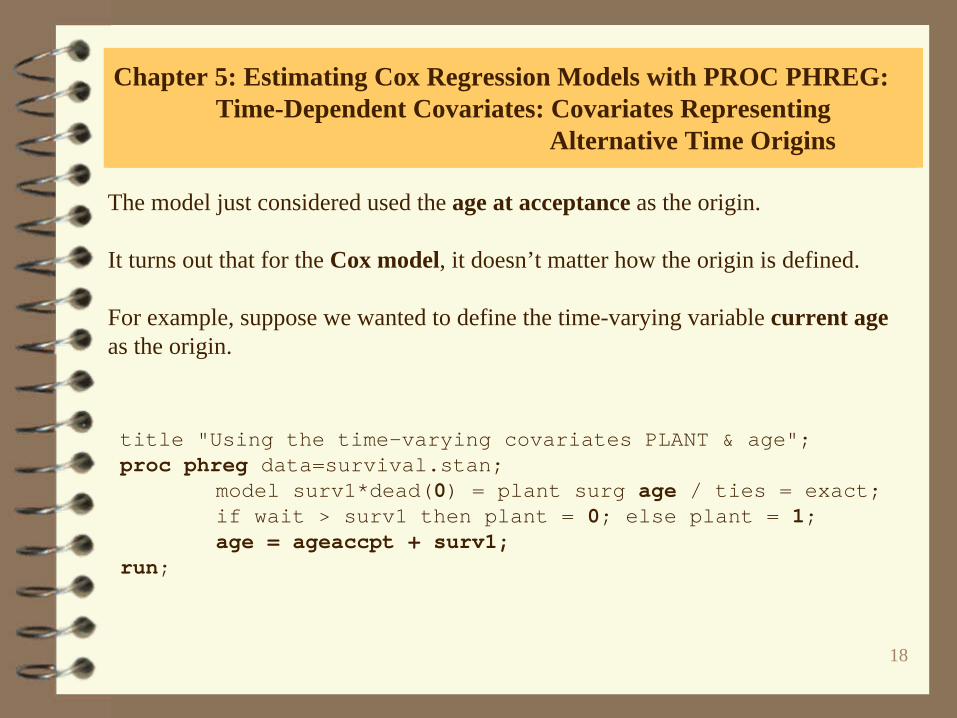
The model just considered used the age at acceptance as the origin.
It turns out that for the Cox model, it doesn’t matter how the origin is defined.
For example, suppose we wanted to define the time-varying variable current age as the origin.
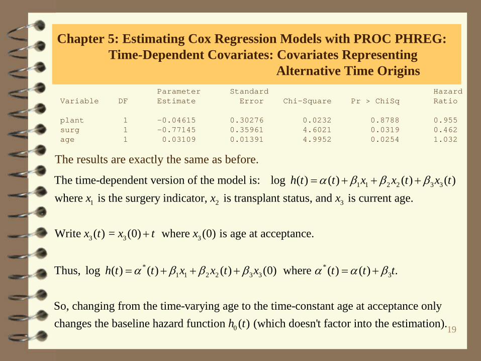
title "Using the time-varying covariates PLANT & age";proc phreg data=survival.stan;
model surv1*dead(0) = plant surg age / ties = exact;if wait > surv1 then plant = 0; else plant = 1;age = ageaccpt + surv1;
run;
19
Chapter 5: Estimating Cox Regression Models with PROC PHREG: Time-Dependent Covariates: Covariates Representing
Alternative Time OriginsParameter Standard Hazard
Variable DF Estimate Error Chi-Square Pr > ChiSq Ratio
plant 1 -0.04615 0.30276 0.0232 0.8788 0.955surg 1 -0.77145 0.35961 4.6021 0.0319 0.462age 1 0.03109 0.01391 4.9952 0.0254 1.032
The results are exactly the same as before.
1 1 2 2 3 3
1 2 3
3 3 3
The time-dependent version of the model is: log ( ) ( ) ( ) ( )where is the surgery indicator, is transplant status, and is current age.
Write ( ) = (0) where (0) is
h t t x x t x tx x x
x t x t x
α β β β= + + +
+
* *1 1 2 2 3 3 3
age at acceptance.
Thus, log ( ) ( ) ( ) (0) where ( ) ( ) .
So, changing from the time-varying age to the time-constant age at acceptance onlychanges the baseline hazard function
h t t x x t x t t tα β β β α α β= + + + = +
0 ( ) (which doesn't factor into the estimation).h t
20
Chapter 5: Estimating Cox Regression Models with PROC PHREG: Time-Dependent Covariates: Covariates Representing
Alternative Time Origins
1 1 2 2 3 3
3 3
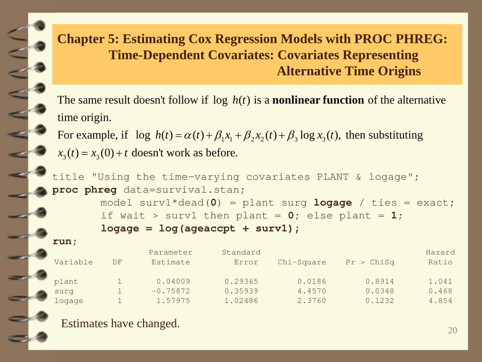
The same result doesn't follow if log ( ) is a of the alternative time origin.For example, if log ( ) ( ) ( ) log ( ), then substituting
( ) (0) doesn't work a
h t
h t t x x t x tx t x t
α β β β= + + += +
nonlinear function
s before.
title "Using the time-varying covariates PLANT & logage";proc phreg data=survival.stan;
model surv1*dead(0) = plant surg logage / ties = exact;if wait > surv1 then plant = 0; else plant = 1;logage = log(ageaccpt + surv1);
run;Parameter Standard Hazard
Variable DF Estimate Error Chi-Square Pr > ChiSq Ratio
plant 1 0.04009 0.29365 0.0186 0.8914 1.041surg 1 -0.75872 0.35939 4.4570 0.0348 0.468logage 1 1.57975 1.02486 2.3760 0.1232 4.854
Estimates have changed.
21
Chapter 5: Estimating Cox Regression Models with PROC PHREG: Time-Dependent Covariates Measured at Regular Intervals
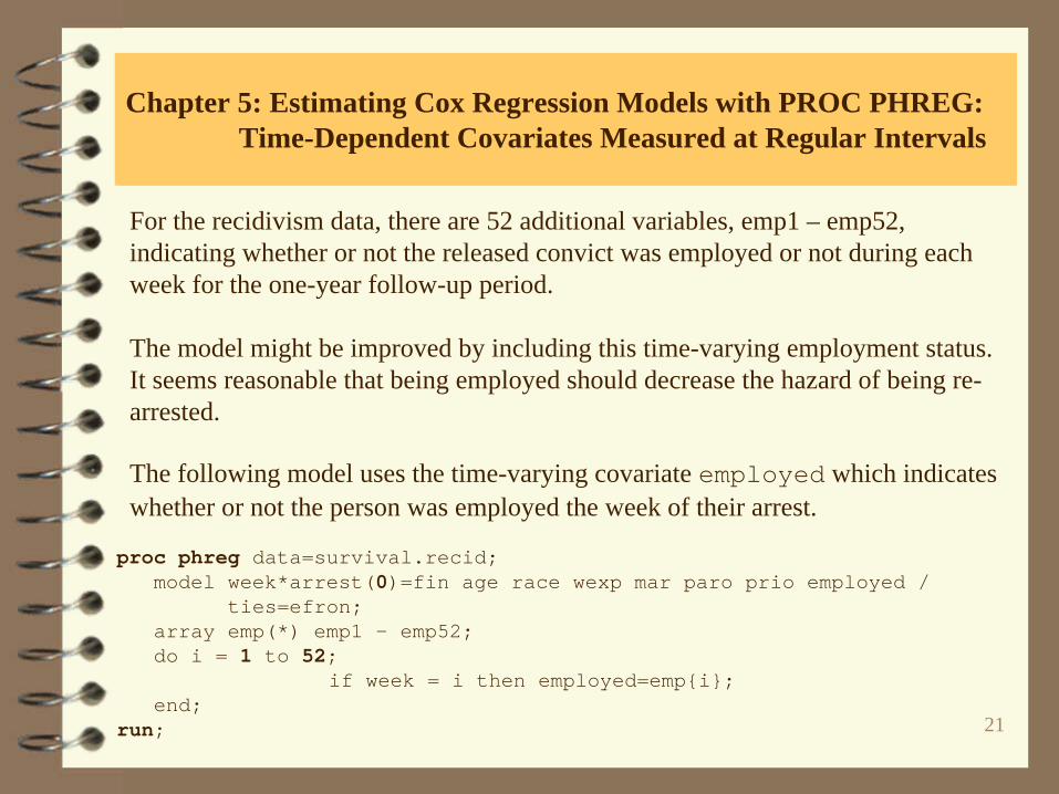
For the recidivism data, there are 52 additional variables, emp1 – emp52, indicating whether or not the released convict was employed or not during each week for the one-year follow-up period.
The model might be improved by including this time-varying employment status.It seems reasonable that being employed should decrease the hazard of being re- arrested.
The following model uses the time-varying covariate employed which indicates whether or not the person was employed the week of their arrest.
proc phreg data=survival.recid;model week*arrest(0)=fin age race wexp mar paro prio employed /
ties=efron;array emp(*) emp1 - emp52;do i = 1 to 52;
if week = i then employed=emp{i};end;
run;
22
Chapter 5: Estimating Cox Regression Models with PROC PHREG: Time-Dependent Covariates Measured at Regular Intervals
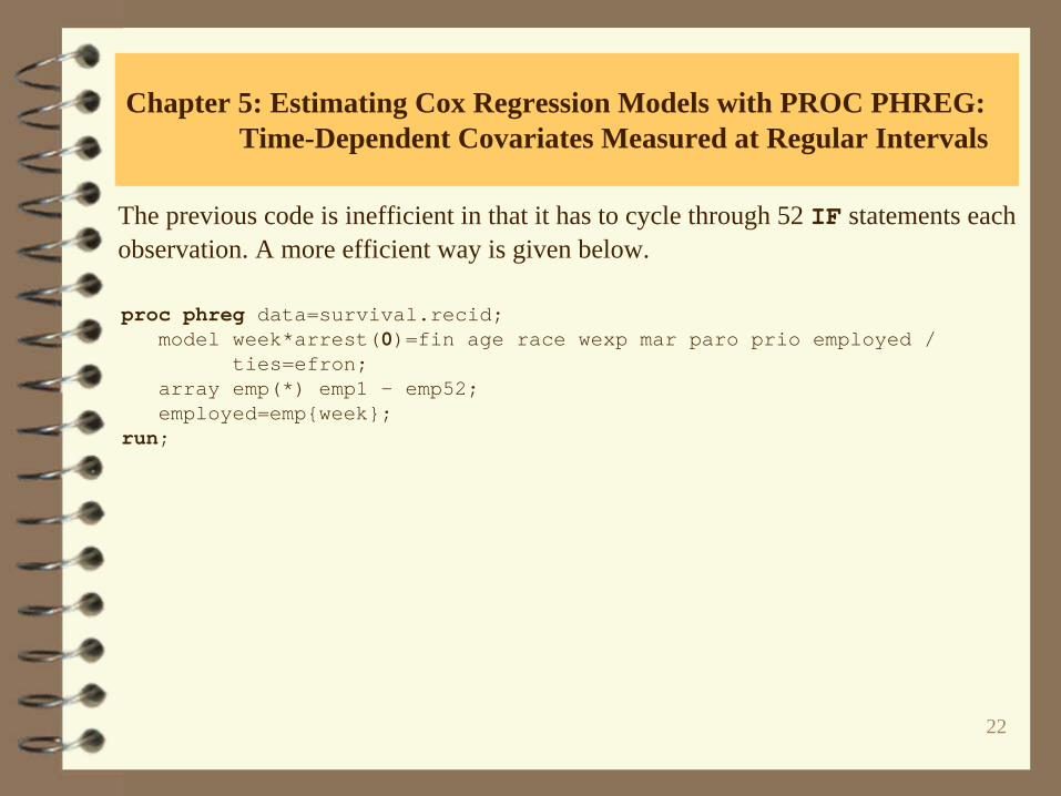
The previous code is inefficient in that it has to cycle through 52 IF statements eachobservation. A more efficient way is given below.
proc phreg data=survival.recid;model week*arrest(0)=fin age race wexp mar paro prio employed /
ties=efron;array emp(*) emp1 - emp52;employed=emp{week};
run;
23
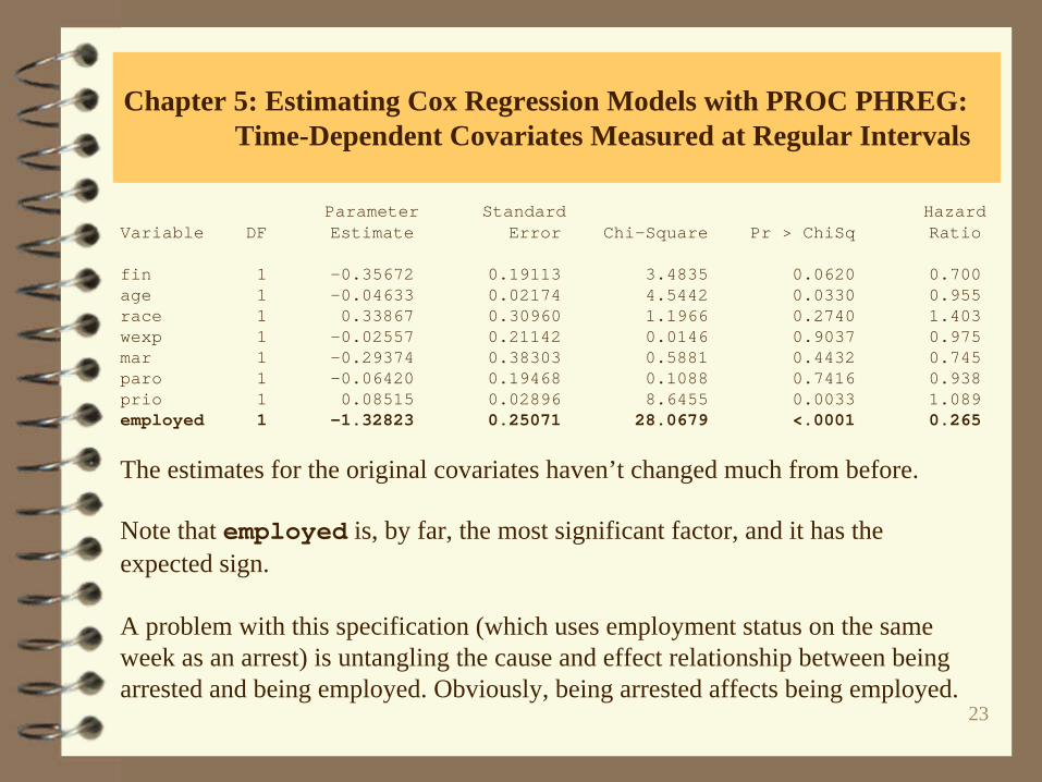
Chapter 5: Estimating Cox Regression Models with PROC PHREG: Time-Dependent Covariates Measured at Regular Intervals
Parameter Standard Hazard Variable DF Estimate Error Chi-Square Pr > ChiSq Ratio
fin 1 -0.35672 0.19113 3.4835 0.0620 0.700age 1 -0.04633 0.02174 4.5442 0.0330 0.955race 1 0.33867 0.30960 1.1966 0.2740 1.403wexp 1 -0.02557 0.21142 0.0146 0.9037 0.975mar 1 -0.29374 0.38303 0.5881 0.4432 0.745paro 1 -0.06420 0.19468 0.1088 0.7416 0.938prio 1 0.08515 0.02896 8.6455 0.0033 1.089employed 1 -1.32823 0.25071 28.0679 <.0001 0.265
The estimates for the original covariates haven’t changed much from before.
Note that employed is, by far, the most significant factor, and it has the expected sign.
A problem with this specification (which uses employment status on the same week as an arrest) is untangling the cause and effect relationship between being arrested and being employed. Obviously, being arrested affects being employed.
24
Chapter 5: Estimating Cox Regression Models with PROC PHREG: Time-Dependent Covariates Measured at Regular Intervals
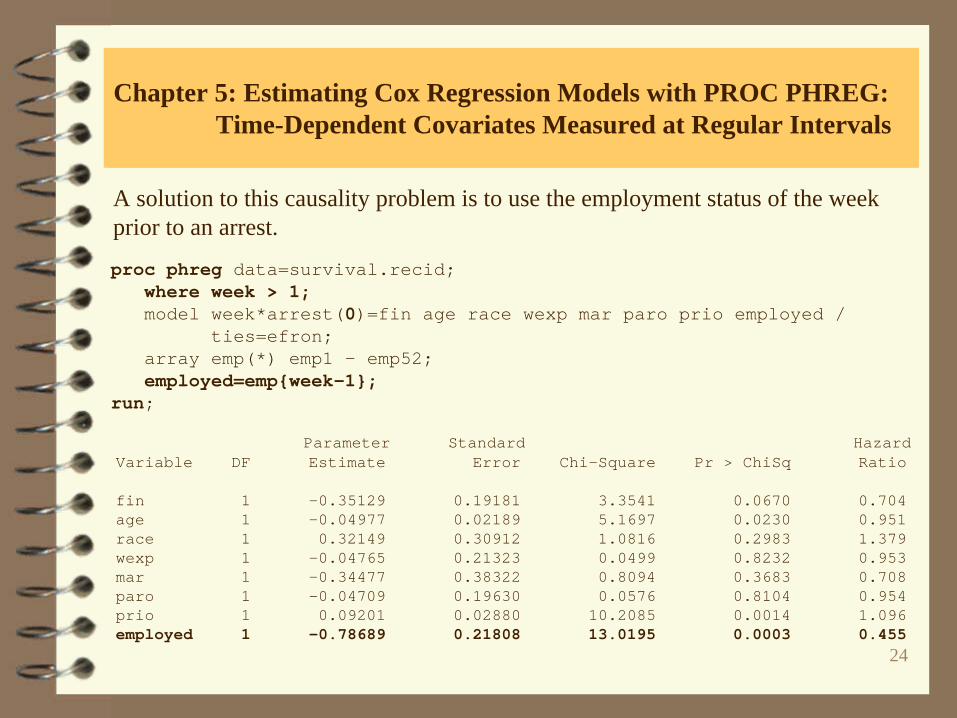
A solution to this causality problem is to use the employment status of the week prior to an arrest.
proc phreg data=survival.recid;where week > 1;model week*arrest(0)=fin age race wexp mar paro prio employed /
ties=efron;array emp(*) emp1 - emp52;employed=emp{week-1};
run;
Parameter Standard HazardVariable DF Estimate Error Chi-Square Pr > ChiSq Ratio
fin 1 -0.35129 0.19181 3.3541 0.0670 0.704age 1 -0.04977 0.02189 5.1697 0.0230 0.951race 1 0.32149 0.30912 1.0816 0.2983 1.379wexp 1 -0.04765 0.21323 0.0499 0.8232 0.953mar 1 -0.34477 0.38322 0.8094 0.3683 0.708paro 1 -0.04709 0.19630 0.0576 0.8104 0.954prio 1 0.09201 0.02880 10.2085 0.0014 1.096employed 1 -0.78689 0.21808 13.0195 0.0003 0.455
25
Chapter 5: Estimating Cox Regression Models with PROC PHREG: Time-Dependent Covariates Measured at Regular Intervals
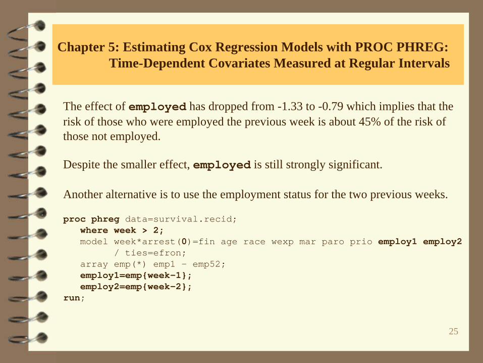
The effect of employed has dropped from -1.33 to -0.79 which implies that the risk of those who were employed the previous week is about 45% of the risk of those not employed.
Despite the smaller effect, employed is still strongly significant.
Another alternative is to use the employment status for the two previous weeks.
proc phreg data=survival.recid;where week > 2;model week*arrest(0)=fin age race wexp mar paro prio employ1 employ2
/ ties=efron;array emp(*) emp1 - emp52;employ1=emp{week-1};employ2=emp{week-2};
run;
26
Chapter 5: Estimating Cox Regression Models with PROC PHREG: Time-Dependent Covariates Measured at Regular Intervals
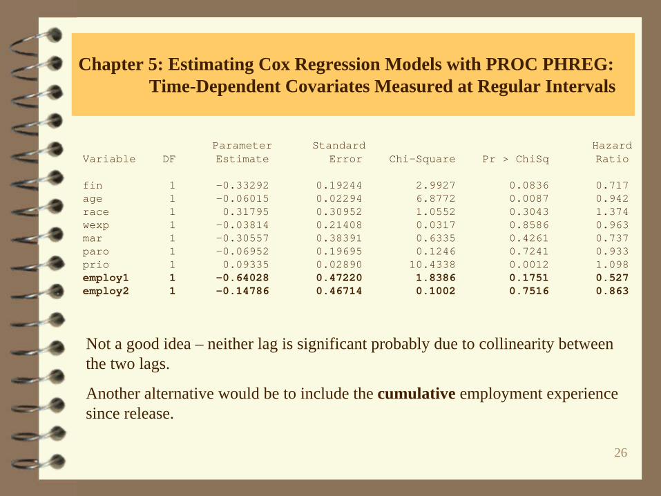
Parameter Standard HazardVariable DF Estimate Error Chi-Square Pr > ChiSq Ratio
fin 1 -0.33292 0.19244 2.9927 0.0836 0.717age 1 -0.06015 0.02294 6.8772 0.0087 0.942race 1 0.31795 0.30952 1.0552 0.3043 1.374wexp 1 -0.03814 0.21408 0.0317 0.8586 0.963mar 1 -0.30557 0.38391 0.6335 0.4261 0.737paro 1 -0.06952 0.19695 0.1246 0.7241 0.933prio 1 0.09335 0.02890 10.4338 0.0012 1.098employ1 1 -0.64028 0.47220 1.8386 0.1751 0.527employ2 1 -0.14786 0.46714 0.1002 0.7516 0.863
Not a good idea – neither lag is significant probably due to collinearity between the two lags.
Another alternative would be to include the cumulative employment experience since release.
27
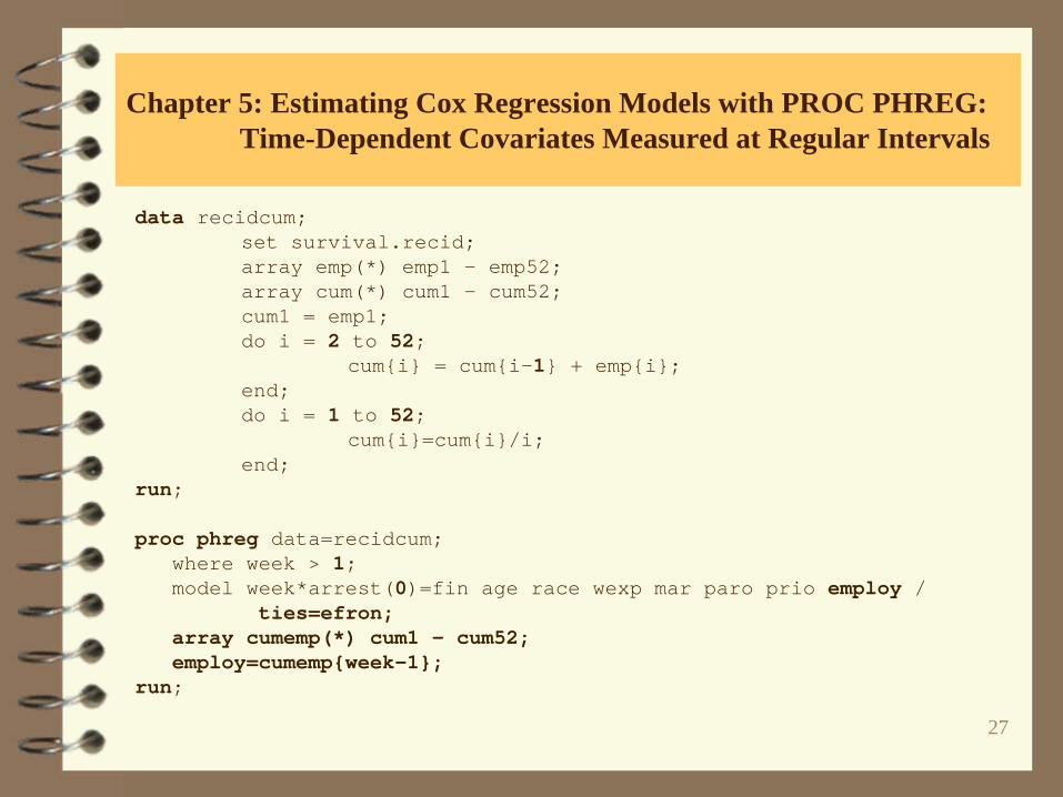
Chapter 5: Estimating Cox Regression Models with PROC PHREG: Time-Dependent Covariates Measured at Regular Intervals
data recidcum;set survival.recid;array emp(*) emp1 - emp52;array cum(*) cum1 - cum52;cum1 = emp1;do i = 2 to 52;
cum{i} = cum{i-1} + emp{i};end;do i = 1 to 52;
cum{i}=cum{i}/i;end;
run;
proc phreg data=recidcum;where week > 1;model week*arrest(0)=fin age race wexp mar paro prio employ /
ties=efron;array cumemp(*) cum1 - cum52;employ=cumemp{week-1};
run;
28
Chapter 5: Estimating Cox Regression Models with PROC PHREG: Time-Dependent Covariates Measured at Regular Intervals
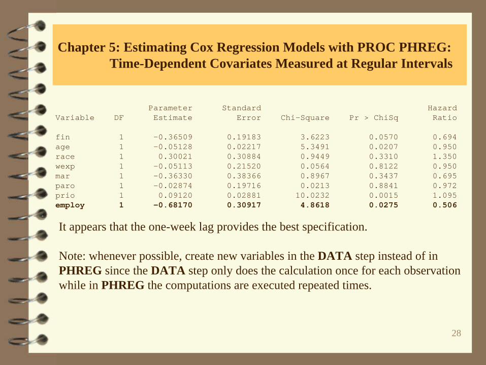
Parameter Standard HazardVariable DF Estimate Error Chi-Square Pr > ChiSq Ratio
fin 1 -0.36509 0.19183 3.6223 0.0570 0.694age 1 -0.05128 0.02217 5.3491 0.0207 0.950race 1 0.30021 0.30884 0.9449 0.3310 1.350wexp 1 -0.05113 0.21520 0.0564 0.8122 0.950mar 1 -0.36330 0.38366 0.8967 0.3437 0.695paro 1 -0.02874 0.19716 0.0213 0.8841 0.972prio 1 0.09120 0.02881 10.0232 0.0015 1.095employ 1 -0.68170 0.30917 4.8618 0.0275 0.506
It appears that the one-week lag provides the best specification.
Note: whenever possible, create new variables in the DATA step instead of in PHREG since the DATA step only does the calculation once for each observation while in PHREG the computations are executed repeated times.
29
Chapter 5: Estimating Cox Regression Models with PROC PHREG: Ad_Hoc Estimates of Time-Dependent Covariates
Suppose we have data on the event of interest at one time-scale and an important time-varying covariate is measured at a different time-scale.
For example, the exact day of death is measured, but albumin level is only measured at the monthly level.
To apply the partial likelihood method, measurements on albumin levels will be needed at the daily level.
Several methods, none of which are perfect, have been suggested for solving this problem.
For the albumin level variable, a reasonable solution would be to use the closest preceding albumin level to impute a daily event time value.
30
Chapter 5: Estimating Cox Regression Models with PROC PHREG: Ad_Hoc Estimates of Time-Dependent Covariates
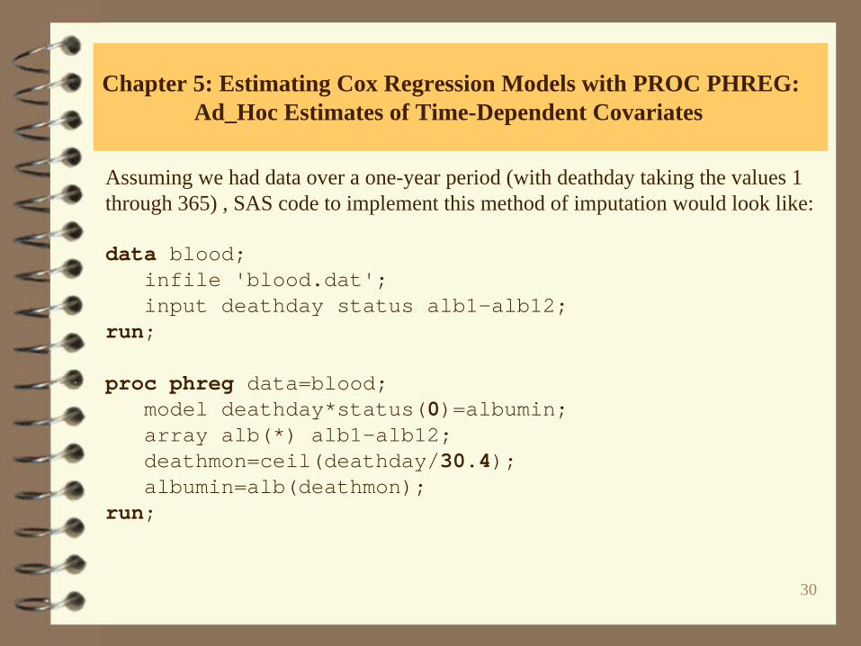
Assuming we had data over a one-year period (with deathday taking the values 1 through 365) , SAS code to implement this method of imputation would look like:
data blood;infile 'blood.dat';input deathday status alb1-alb12;
run;
proc phreg data=blood;model deathday*status(0)=albumin;array alb(*) alb1-alb12;deathmon=ceil(deathday/30.4);albumin=alb(deathmon);
run;
31
Chapter 5: Estimating Cox Regression Models with PROC PHREG: Ad_Hoc Estimates of Time-Dependent Covariates
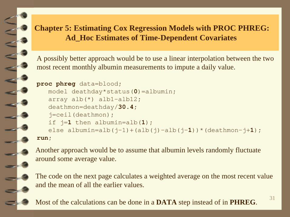
A possibly better approach would be to use a linear interpolation between the two most recent monthly albumin measurements to impute a daily value.
proc phreg data=blood;model deathday*status(0)=albumin;array alb(*) alb1-alb12;deathmon=deathday/30.4;j=ceil(deathmon);if j=1 then albumin=alb(1);else albumin=alb(j-1)+(alb(j)-alb(j-1))*(deathmon-j+1);
run;
Another approach would be to assume that albumin levels randomly fluctuate around some average value.
The code on the next page calculates a weighted average on the most recent value and the mean of all the earlier values.
Most of the calculations can be done in a DATA step instead of in PHREG.
32
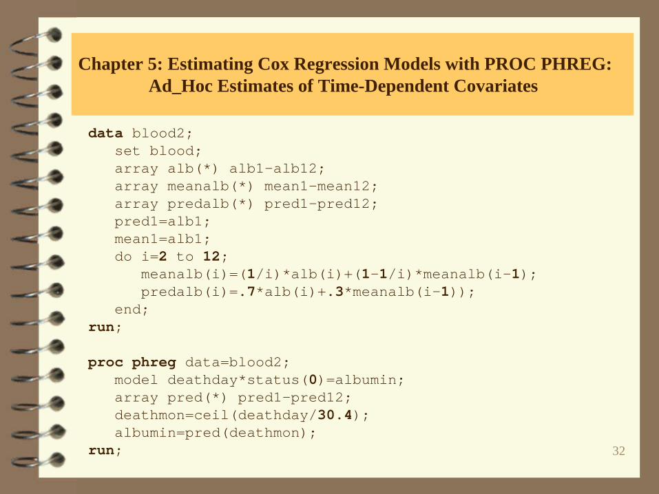
Chapter 5: Estimating Cox Regression Models with PROC PHREG: Ad_Hoc Estimates of Time-Dependent Covariates
data blood2;set blood;array alb(*) alb1-alb12;array meanalb(*) mean1-mean12;array predalb(*) pred1-pred12;pred1=alb1;mean1=alb1;do i=2 to 12;
meanalb(i)=(1/i)*alb(i)+(1-1/i)*meanalb(i-1);predalb(i)=.7*alb(i)+.3*meanalb(i-1));
end;run;
proc phreg data=blood2;model deathday*status(0)=albumin;array pred(*) pred1-pred12;deathmon=ceil(deathday/30.4);albumin=pred(deathmon);
run;
33
Chapter 5: Estimating Cox Regression Models with PROC PHREG: Time-Dependent Covariates that Change at Irregular Intervals
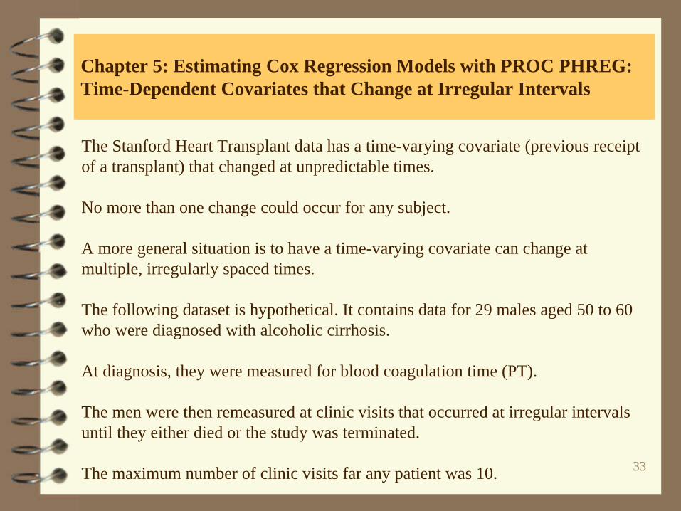
The Stanford Heart Transplant data has a time-varying covariate (previous receipt of a transplant) that changed at unpredictable times.
No more than one change could occur for any subject.
A more general situation is to have a time-varying covariate can change at multiple, irregularly spaced times.
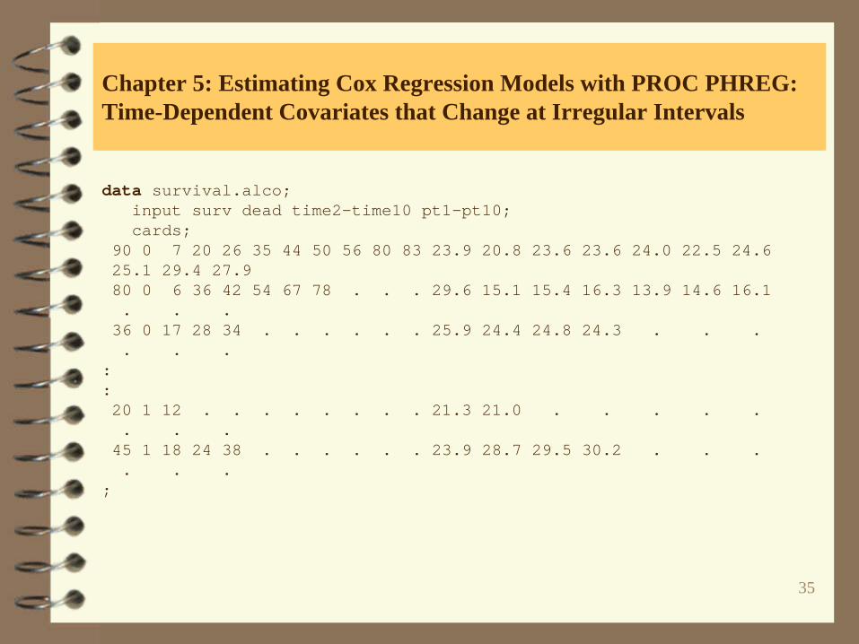
The following dataset is hypothetical. It contains data for 29 males aged 50 to 60 who were diagnosed with alcoholic cirrhosis.
At diagnosis, they were measured for blood coagulation time (PT).
The men were then remeasured at clinic visits that occurred at irregular intervals until they either died or the study was terminated.
The maximum number of clinic visits far any patient was 10.
34
Chapter 5: Estimating Cox Regression Models with PROC PHREG: Time-Dependent Covariates that Change at Irregular Intervals
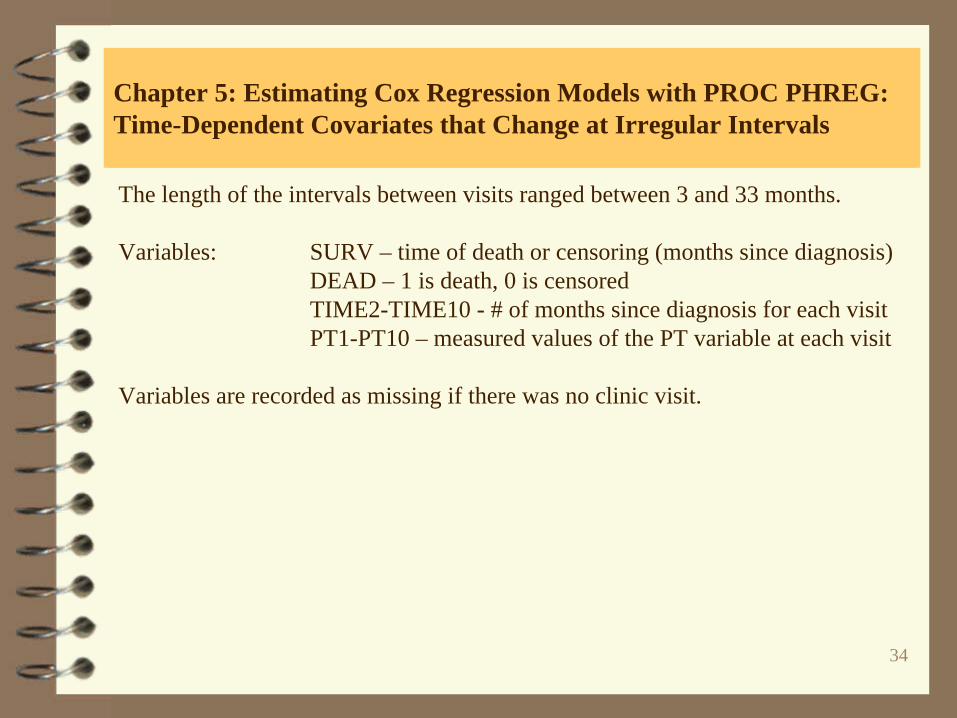
The length of the intervals between visits ranged between 3 and 33 months.
Variables: SURV – time of death or censoring (months since diagnosis)DEAD – 1 is death, 0 is censoredTIME2-TIME10 - # of months since diagnosis for each visitPT1-PT10 – measured values of the PT variable at each visit
Variables are recorded as missing if there was no clinic visit.
35
Chapter 5: Estimating Cox Regression Models with PROC PHREG: Time-Dependent Covariates that Change at Irregular Intervals
data survival.alco;input surv dead time2-time10 pt1-pt10;cards;
90 0 7 20 26 35 44 50 56 80 83 23.9 20.8 23.6 23.6 24.0 22.5 24.625.1 29.4 27.980 0 6 36 42 54 67 78 . . . 29.6 15.1 15.4 16.3 13.9 14.6 16.1. . .
36 0 17 28 34 . . . . . . 25.9 24.4 24.8 24.3 . . .. . .
::20 1 12 . . . . . . . . 21.3 21.0 . . . . .. . .
45 1 18 24 38 . . . . . . 23.9 28.7 29.5 30.2 . . .. . .
;
36
Chapter 5: Estimating Cox Regression Models with PROC PHREG: Time-Dependent Covariates that Change at Irregular Intervals
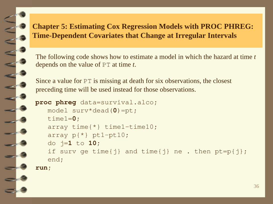
The following code shows how to estimate a model in which the hazard at time t depends on the value of PT at time t.
Since a value for PT is missing at death for six observations, the closest preceding time will be used instead for those observations.
proc phreg data=survival.alco;model surv*dead(0)=pt;time1=0;array time{*} time1-time10;array p{*} pt1-pt10;do j=1 to 10;if surv ge time{j} and time{j} ne . then pt=p{j};end;
run;
37
Chapter 5: Estimating Cox Regression Models with PROC PHREG: Time-Dependent Covariates that Change at Irregular Intervals
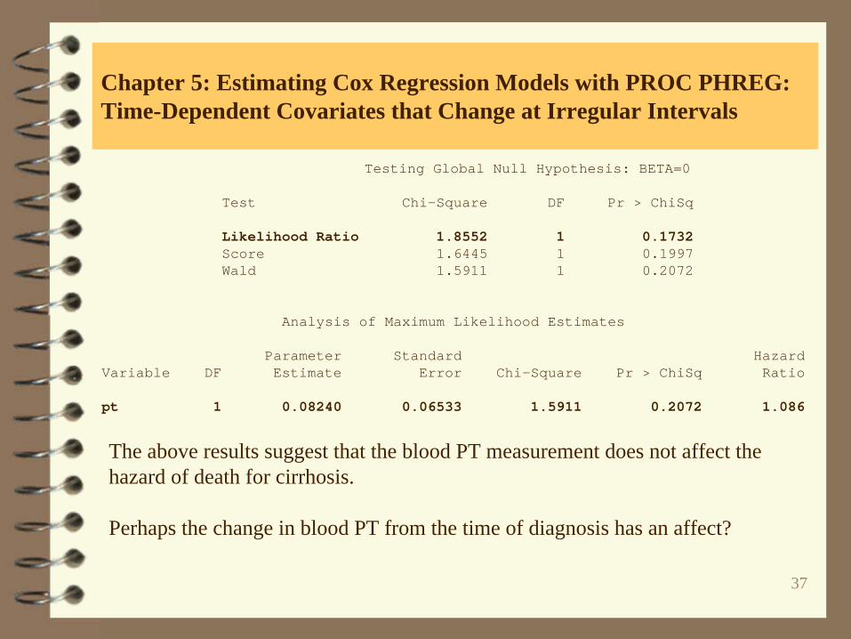
Testing Global Null Hypothesis: BETA=0
Test Chi-Square DF Pr > ChiSq
Likelihood Ratio 1.8552 1 0.1732Score 1.6445 1 0.1997Wald 1.5911 1 0.2072
Analysis of Maximum Likelihood Estimates
Parameter Standard HazardVariable DF Estimate Error Chi-Square Pr > ChiSq Ratio
pt 1 0.08240 0.06533 1.5911 0.2072 1.086
The above results suggest that the blood PT measurement does not affect the hazard of death for cirrhosis.
Perhaps the change in blood PT from the time of diagnosis has an affect?

38
Chapter 5: Estimating Cox Regression Models with PROC PHREG: Time-Dependent Covariates that Change at Irregular Intervals
proc phreg data=survival.alco;model surv*dead(0)=pt;time1=0;array time{*} time1-time10;array p{*} pt1-pt10;do j=1 to 10;if surv ge time{j} and time{j} ne . then pt=p{j} – pt1;end;
run; Testing Global Null Hypothesis: BETA=0
Test Chi-Square DF Pr > ChiSq
Likelihood Ratio 6.9209 1 0.0085Score 3.6743 1 0.0553Wald 5.6300 1 0.0177
Analysis of Maximum Likelihood EstimatesParameter Standard Hazard
Variable DF Estimate Error Chi-Square Pr > ChiSq Ratio
pt 1 0.34844 0.14685 5.6300 0.0177 1.417
Much better!!
39
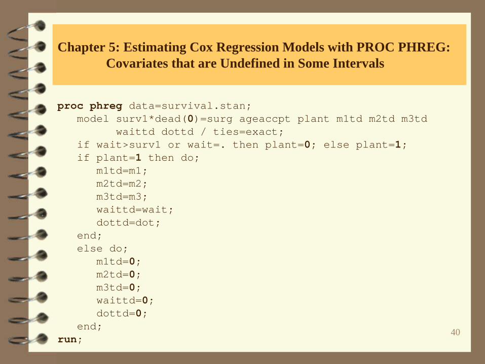
Chapter 5: Estimating Cox Regression Models with PROC PHREG: Covariates that are Undefined in Some Intervals
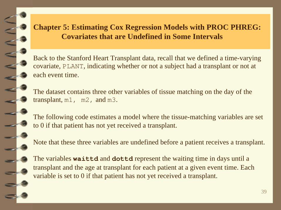
Back to the Stanford Heart Transplant data, recall that we defined a time-varying covariate, PLANT, indicating whether or not a subject had a transplant or not at each event time.
The dataset contains three other variables of tissue matching on the day of the transplant, m1, m2, and m3.
The following code estimates a model where the tissue-matching variables are set to 0 if that patient has not yet received a transplant.
Note that these three variables are undefined before a patient receives a transplant.
The variables waittd and dottd represent the waiting time in days until a transplant and the age at transplant for each patient at a given event time. Each variable is set to 0 if that patient has not yet received a transplant.
40
Chapter 5: Estimating Cox Regression Models with PROC PHREG: Covariates that are Undefined in Some Intervals
proc phreg data=survival.stan;model surv1*dead(0)=surg ageaccpt plant m1td m2td m3td
waittd dottd / ties=exact;if wait>surv1 or wait=. then plant=0; else plant=1;if plant=1 then do;
m1td=m1;m2td=m2;m3td=m3;waittd=wait;dottd=dot;
end;else do;
m1td=0;m2td=0;m3td=0;waittd=0;dottd=0;
end;run;
41
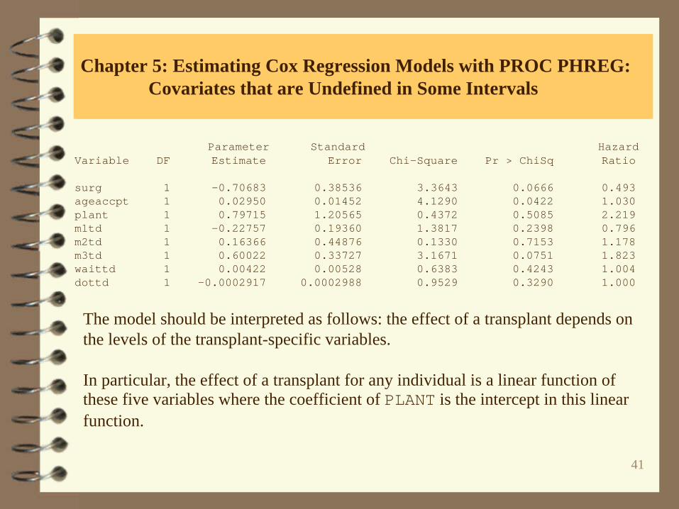
Chapter 5: Estimating Cox Regression Models with PROC PHREG: Covariates that are Undefined in Some Intervals
Parameter Standard HazardVariable DF Estimate Error Chi-Square Pr > ChiSq Ratio
surg 1 -0.70683 0.38536 3.3643 0.0666 0.493ageaccpt 1 0.02950 0.01452 4.1290 0.0422 1.030plant 1 0.79715 1.20565 0.4372 0.5085 2.219m1td 1 -0.22757 0.19360 1.3817 0.2398 0.796m2td 1 0.16366 0.44876 0.1330 0.7153 1.178m3td 1 0.60022 0.33727 3.1671 0.0751 1.823waittd 1 0.00422 0.00528 0.6383 0.4243 1.004dottd 1 -0.0002917 0.0002988 0.9529 0.3290 1.000
The model should be interpreted as follows: the effect of a transplant depends on the levels of the transplant-specific variables.
In particular, the effect of a transplant for any individual is a linear function of these five variables where the coefficient of PLANT is the intercept in this linear function.