Review Article

Susceptibility-Weighted Imaging and QuantitativeSusceptibility Mapping in the Brain

Chunlei Liu, PhD,1,2* Wei Li, PhD,3,4 Karen A. Tong, MD,5 Kristen W. Yeom, MD,6

and Samuel Kuzminski, MD2

Susceptibility-weighted imaging (SWI) is a magnetic reso-nance imaging (MRI) technique that enhances image con-trast by using the susceptibility differences betweentissues. It is created by combining both magnitude andphase in the gradient echo data. SWI is sensitive to bothparamagnetic and diamagnetic substances which gener-ate different phase shift in MRI data. SWI images can bedisplayed as a minimum intensity projection that provideshigh resolution delineation of the cerebral venous archi-tecture, a feature that is not available in other MRI tech-niques. As such, SWI has been widely applied to diagnosevarious venous abnormalities. SWI is especially sensitiveto deoxygenated blood and intracranial mineral depositionand, for that reason, has been applied to image variouspathologies including intracranial hemorrhage, traumaticbrain injury, stroke, neoplasm, and multiple sclerosis.SWI, however, does not provide quantitative measures ofmagnetic susceptibility. This limitation is currently beingaddressed with the development of quantitative suscepti-bility mapping (QSM) and susceptibility tensor imaging(STI). While QSM treats susceptibility as isotropic, STItreats susceptibility as generally anisotropic characterizedby a tensor quantity. This article reviews the basic princi-ples of SWI, its clinical and research applications, themechanisms governing brain susceptibility properties,and its practical implementation, with a focus on brainimaging.

Key Words: MRI, magnetic resonance imaging; SWI, sus-ceptibility weighted imaging; STI, susceptibility tensorimaging; QSM, quantitative susceptibility mapping; MSA,magnetic susceptibility anisotropy; hemorrhage; iron;myelin; TBI, traumatic brain injury; multiple sclerosis;stroke

J. Magn. Reson. Imaging 2015;42:23–41.VC 2014 Wiley Periodicals, Inc.

TRADITIONALLY, magnetic susceptibility-inducedfield perturbation is mostly regarded as a source ofimage artifacts in magnetic resonance imaging (MRI).This treatment is warranted, as no usable soft-tissuecontrast is readily available from this perturbationand large field offset creates various unwanted distor-tions in MRI images. However, magnetic susceptibilityis also an intrinsic property of tissue. If treated prop-erly, it can provide important information about tis-sue structure and function.

Susceptibility-weighted imaging (SWI) is one suchtechnique that takes advantage of the magnetic prop-erty to create useful image contrast (1–3). SWI com-bines a T2*-weighted magnitude image with a filteredphase image acquired with the gradient echo sequencein a multiplicative relationship (1,3). While the T2*-weighted magnitude image already provides some sus-ceptibility contrast, SWI further enhances the contrastbetween tissues of differing susceptibility. In the pastdecade, SWI has found a growing number of applica-tions in the brain and is being gradually adopted inroutine clinical imaging. SWI, however, does not pro-vide quantitative measures of magnetic susceptibility.This limitation is being addressed with the recentdevelopment of quantitative susceptibility mapping(QSM) (4–34) and susceptibility tensor imaging (STI)(18,35–46). While SWI generates contrast based onphase images, QSM further computes the underlyingsusceptibility of each voxel as a scalar quantity. STI, onthe other hand, treats susceptibility as a tensor (i.e., a3 � 3 matrix) quantity rather than a scalar quantity,which allows the quantification of magnetic suscepti-bility anisotropy (MSA) (35).

The purpose of this review is to provide an overviewof the basic principles of susceptibility imaging, the

1Brain Imaging and Analysis Center, School of Medicine, DukeUniversity, Durham, North Carolina, USA.2Department of Radiology, School of Medicine, Duke University,Durham, North Carolina, USA.3Research Imaging Institute, University of Texas Health ScienceCenter at San Antonio, Texas, USA.4Department of Ophthalmology, University of Texas Health ScienceCenter at San Antonio, Texas, USA.5Department of Radiology, School of Medicine, Loma LindaUniversity, Loma Linda, California, USA.6Department of Radiology, Lucile Packard Children’s Hospital,Stanford University, Palo Alto, California, USA.

Contract grant sponsor: National Institutes of Health; Contract grantnumbers: R01MH096979, R13EB018725, P41EB015897; Contractgrant sponsor: National Multiple Sclerosis Society; Contract grantnumber: RG4723.

*Address reprint requests to: C.L., Brain Imaging and Analysis Cen-ter, Duke University School of Medicine, 2424 Erwin Road, Suite501, Campus Box 2737, Durham, NC 27705.E-mail: chunlei.liu@duke.edu

Received April 29, 2014; Accepted September 5, 2014.

DOI 10.1002/jmri.24768View this article online at wileyonlinelibrary.com.

JOURNAL OF MAGNETIC RESONANCE IMAGING 42:23–41 (2015)

CME

VC 2014 Wiley Periodicals, Inc. 23

mechanisms governing brain susceptibility properties,corresponding clinical and research applications, andaspects of its practical implementation. All three tech-niques of SWI, QSM, and STI are reviewed, as they areclosely related. Because of the rapid development ofthese techniques, this limited review cannot exhaus-tively cover all aspects of the field. Rather, we intend tofocus on the basic principles and illustrate their appli-cations with some examples, which can potentiallyserve a foundation for more in-depth studies.

MAGNETIC SUSCEPTIBILITY AND GRADIENT ECHO

Magnetic susceptibility is a physical quantity that meas-ures the extent to which a material is magnetized by anapplied magnetic field. While magnetic susceptibility ingeneral includes both static and AC susceptibility, whatis described here is the susceptibility in response to thestatic B0 field. Susceptibility of a material, noted by x, isequal to the ratio of the magnetization, M, within thematerial to the strength of the applied magnetic field, H,i.e., x ¼ M/H. In MRI images, this defines the volumesusceptibility (dimensionless in SI units). Magneticmaterials are classically designated as diamagnetic,paramagnetic, or ferromagnetic. Diamagnetic materialshave negative susceptibility while paramagnetic materi-als have positive susceptibility. Biological tissues can beeither diamagnetic or paramagnetic depending on theirmolecular contents and microstructure. Water, the mostabundant molecule in the brain, has a volume suscepti-bility of –9.035 � 10�6 (or –9.035 ppm) (SI units) (47),while the variations of susceptibility among brain tis-sues relative to water is generally small, on the order of60.1 ppm (9,10,15,25,48). In comparison, susceptibil-ity of the air is about 0.37 ppm (SI units) (49). Becauseproton MRI signal is referenced to the Larmor frequency,mainly of water, the field perturbation and frequency

shift within the brain are largely due to the significantlydifferent susceptibilities between tissue and air cavitiesnear the brain such as the nasal cavity and ear canals.Contrary to the signal of MRI, which originates fromnuclear magnetization, the dominant magnetizationthat contributes to magnetic susceptibility originatesfrom orbital electrons.

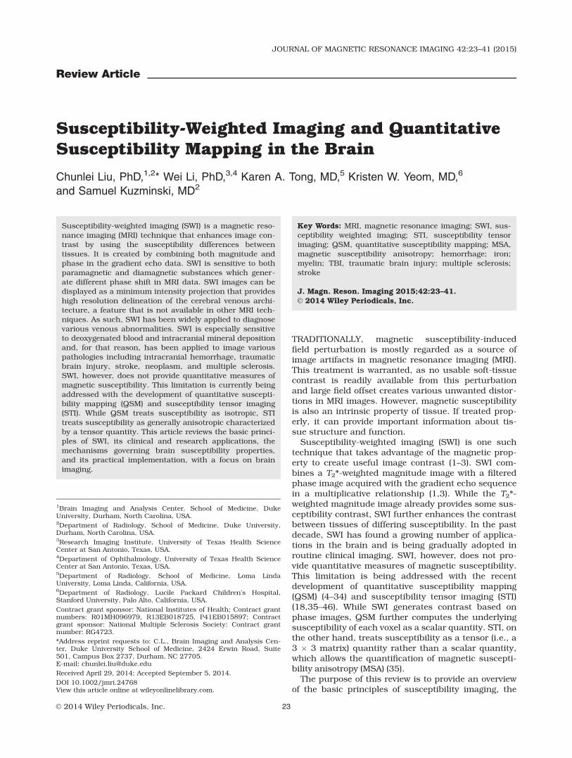
The most commonly used sequence for visualizingthe effect of magnetic susceptibility is the spoiledgradient-recalled-echo (SPGR or GRE) sequence (Fig.1), which can be of a single echo or multiple echoes, 2Dor 3D. The magnitude of a series of multiecho GREimages exhibits a single exponential or multiexponen-tial decay (T2* decay). The phase (Q) of GRE imagesmeasures local frequency offset (f) relative to the Lar-mor frequency, which reflects the mean magnetic fieldperturbation seen by spins within a voxel, following therelationship of Q ¼ –2p ft in a right-hand coordinatesystem. In this coordinate system, spins with positivegyromagnetic ratio (e.g., protons) rotate clockwise look-ing down, thus the negative sign (50). The T2* decayconstant is primarily determined by a combination offield inhomogeneities and spin–spin relaxation (T2).The relationship is typically expressed as R2* ¼ 1/T2*¼ 1/T2 þ gDB/2 or R�2 ¼ R2 þ R

02, where g is the gyro-

magnetic ratio, DB is the full width at half maximum(FWHM) of the field distribution, and R2 ¼ 1/T2.

PRINCIPLES OF MAGNETIC SUSCEPTIBILITY IMAGING

Phase Maps of Gradient Echo

The most severe and obvious artifact in the phase of agradient echo is the discontinuity caused by phasewrapping (Fig. 1). Phase wrapping occurs becausesine and cosine functions are periodic with a period of2p. Any angle outside the range between –p and p willbe folded back. In addition, the phase value within

Figure 1. A spoiled multiecho gradient echo sequence. Alternating readout polarities are illustrated, although single polaritymay also be used. Flow compensation may also be added. The contrast in the magnitude images evolve as the echo timeincreases due to T2* decay. Phase values increase as TE increases, thus more phase wraps appear at later echoes. Phase con-trast between gray and white matter is still observable under these phase wraps. SWI and QSM may use either single or mul-tiple echoes.

24 Liu et al.

the brain is also influenced by the phase of thereceiver coils, the long-range magnetic field (dipolefield) generated by the human body itself, and thelarge susceptibility difference between tissue and air.Phase contributed by sources outside a region ofinterest is commonly referred to as the “backgroundphase.” The presence of large background phase notonly disguises local tissue contrast, but also worsensphase wrapping. A common approach in using phaseis to perform a phase unwrapping procedure followedby a highpass filtering operation with the assumptionthat the background phase is smooth, containing onlylow spatial frequencies (1–3).

A variety of phase unwrapping and backgroundphase removal approaches have been proposed. Forexample, phase unwrapping can be achieved usingconventional path-based methods in the spatialdomain and linear fitting methods in the temporaldomain (51,52). The difficulty of phase unwrappingcan be further compounded by the low signal-to-noiseratio (SNR) (52). The goal of background phaseremoval is to separate the background phase fromphase contributed by brain tissue itself. Traditionalhighpass filtering, e.g., homodyne filtering, that hasbeen successfully used in SWI, can remove, alongwith the background phase, a substantial portion oflow-frequency components of the tissue phase. Thiswill inevitably lead to inaccurate susceptibility quanti-fication. A number of viable solutions have beendeveloped recently that can more accurately separate

background phase from tissue phase. These methodsinclude, for example, the sophisticated harmonic arti-fact reduction for phase data (SHARP) method and itsvariants (9,11,28,48), the projection onto dipole fields(PDF) method (53), and harmonic phase removalusing the Laplacian operator (HARPERELLA) (23).Particularly, HARPERELLA achieves phase unwrap-ping and background removal simultaneously.

The value of gradient echo phase was recognizedearly. For example, Young et al (6) used the fieldeffects to detect changes in tumors, hematomas, lacu-nar infarct, and multiple sclerosis; Glover (54) usedthe susceptibility effect to improve the Dixon tech-nique; Conturo et al (55) used the phase to quantifyGd perfusion; filtered phase images also revealeddetailed neural anatomy (56,57).

Susceptibility-Weighted Imaging

The central idea of SWI is to enhance susceptibility-induced contrast by combining both magnitude andphase. Magnitude or phase by itself only uses half theacquired information. de Crespigny et al (2) proposeda technique that improved the sensitivity to suscepti-bility contrast by combining both. They proposed thatamplitude and phase could be combined in a numberof ways so that they enhanced each other, rather thancanceled out and demonstrated one simple approachto reconstruct the real images mag�cos(Q) after

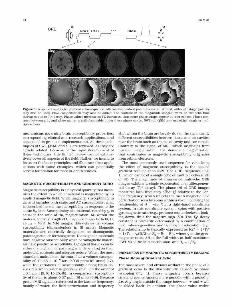
Figure 2. Flowcharts of processing steps of SWI (a) and QSM (b). (a) SWI combines both the magnitude and a filtered phasemap in a multiplicative relationship to enhance image contrast. Minimum intensity projection (MIP) is commonly applied tohighlight the veins. The contrast can be adjusted by varying the number of slices used in MIP (examples shown in later fig-ures). SWI flowchart adapted from Reichenbach et al (3). (b) There are two major steps involved in QSM: filtering backgroundphase and solving an inverse problem.

Brain Susceptibility Imaging and Mapping 25

appropriate phase correction to account for variousstatic phase variations.

SWI, as commonly used today (Fig. 2a), was des-cribed by Reichenbach et al (3) as “MR Venography.”The main goal was to enhance the visualization of smallvessels by taking advantage of the paramagnetic prop-erty of deoxyhemoglobin. Cho et al (58) developed a“NMR Venography” that used the susceptibility effect ofdeoxyhemoglobin. Cho et al relied on the magnitudeimage generated by a tailored radiofrequency (RF) pulsethat suppressed normal tissues while enhancing thesignals from blood interfaces, where strongsusceptibility-induced fields were present.

The venography technique described by Reichen-bach and colleagues was further generalized in thearticle entitled “Susceptibility weighted imaging” (1).As illustrated in Fig. 2a, in creating SWI, the phaseimage is highpass-filtered and then transformed to aphase mask that varies in amplitude between zeroand one. This mask is multiplied a few times with theoriginal magnitude image to create enhanced contrastbetween tissues of different susceptibilities. The num-ber of phase mask multiplications can be varieddepending on the phase difference and contrast-to-noise ratio, although four multiplications are consid-ered the standard. Haacke et al (1) demonstrated thatSWI could be used for enhancing gray matter / whitematter (GM/WM) contrast, water/fat contrast, andidentifying brain iron, thus extending its applicationbeyond visualizing veins in the brain.

Quantitative Susceptibility Mapping

One intrinsic limitation of signal phase is that phase isnonlocal and orientation-dependent, thus not easilyreproducible. For example, the phase of a vein can beeither positive or negative depending on its orientationwith respect to the B0 field (59). As a result, the appear-ance of a vein can vary in SWI images. Furthermore, it

is difficult and not always reliable to differentiate dia-magnetic susceptibility from paramagnetic susceptibil-ity based on phase or SWI, due to the convoluting effectof the dipole fields. As such, separating calcificationwhich is diamagnetic from iron deposition which isparamagnetic is often challenging in SWI (16). There-fore, it is of great interest to determine the intrinsicproperty of the tissue, i.e., the magnetic susceptibility,from the measured signal phase (Fig. 2b).

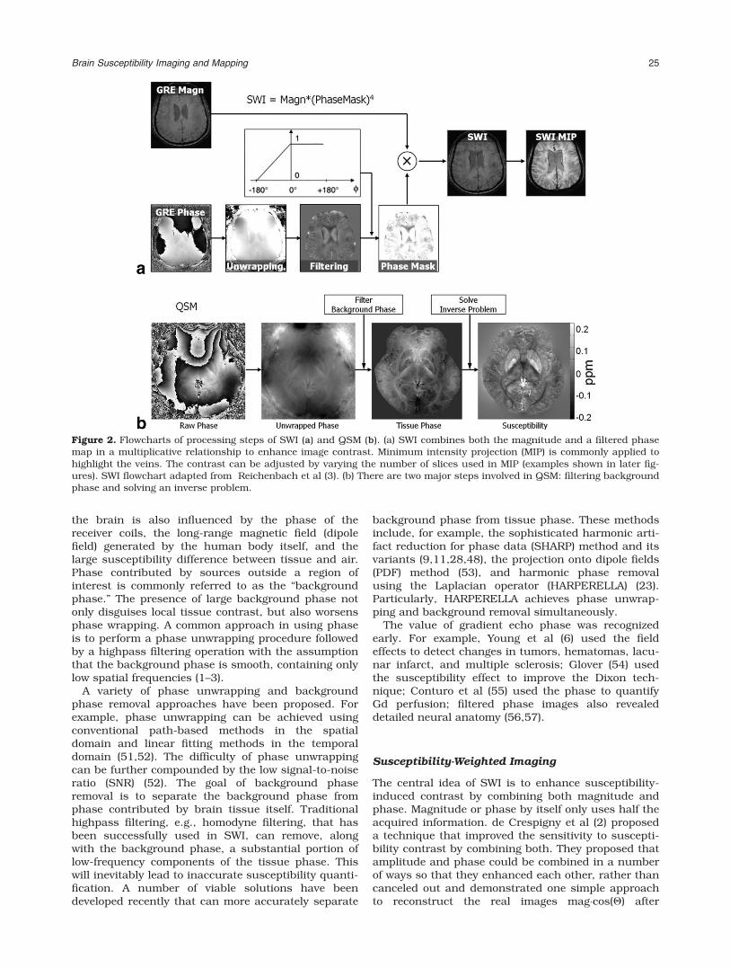
In a simple model where the magnetization of animaging voxel is treated as a magnetic dipole, eachdipole will produce a magnetic field (dipole field) thatspatially extends beyond that voxel itself (Fig. 3a). Themagnetic field at any given voxel is thus a superposi-tion of all dipole fields generated by surrounding vox-els. Because the superposition of magnetic field islinear and the field of a unit dipole is shift invariant(i.e., it does not change from one voxel to another), therelationship between the spatial distribution of suscep-tibility (which is proportional to magnetization) and thespatial distribution of frequency (which is proportionalto magnetic field) is governed by a simple convolution.The impulse response function is the unit dipole field.Convolution in the image domain can be alsoexpressed as multiplication in the k-space (13,14):

f ðkÞ ¼ gB0ð1

3� k2

z

k2ÞxðkÞ [1]

Here, k is the k-space vector and kz is itsz-component; f(k) is the Fourier transform of the mapof frequency offsets f(r); B0 is the magnetic flux den-sity corresponding to the applied magnetic field H0 invaccum; x(k) is the Fourier transform of the suscepti-bility distribution x(r); g is gyromagnetic ratio. Notethat only the z-component of the susceptibility-induced field perturbation is measurable in the fre-quency shift.

Mapping susceptibility requires solving the linearequation shown in Eq. (1) where f(k) is the experimental

Figure 3. Relationship between susceptibility and magnetic field. (a) Each image voxel can be approximated as a magneticdipole which produces a dipole field that extends beyond the voxel itself. Dipole fields originating from different voxels followthe superposition rule resulting in a convolution relationship between field and susceptibility which can be expressed as amultiplication in the k-space. (b) Solving the inverse problem from field to susceptibility is ill-posed, as the coefficients of theequation become zero on a surface of cone in the k-space when k2 ¼ 3k2

z.

26 Liu et al.

measurement and x(k) is the unknown. Inverting Eq.(1) is problematic when k2 ¼ 3k2

z (a conical surface ink-space) as the coefficient becomes zero (Fig. 3b). Con-sequently, x(k) cannot be accurately determined inregions near the conical surfaces. A variety ofapproaches have been proposed to address this issue.These techniques are generally called quantitative sus-ceptibility mapping (QSM). A number of QSM algo-rithms have been developed (4–15). There are softwarepackages now available for research purposes, forexample, MEDI (12) and STI Suite (23). As a conven-tion, all susceptibility maps will be displayed withbrighter intensity representing paramagnetic suscepti-bility and dark intensity representing diamagnetic sus-ceptibility (Fig. 3). One exception is when visualizingsusceptibility anisotropy of white matter, in which casethe intensity scale is flipped (Fig. 4).

Susceptibility Tensor Imaging

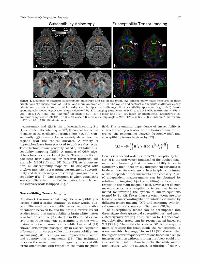
Equation (1) assumes that magnetic susceptibility isisotropic and a scalar quantity; in other words, sus-ceptibility shall not vary with respect to the relativeorientation between B0 and the brain. However, recentstudies found that susceptibility of brain white matteris in fact anisotropic (Fig. 4a,c). Liu (35) found exten-sive anisotropic magnetic susceptibility in the whitematter of intact mouse brains while Lee et al (41)showed anisotropic susceptibility in excised segmentsof human brain corpus callosum. A susceptibility ten-sor imaging (STI) technique was proposed to measureand quantify this phenomenon (35). This techniquerelies on the measurement of frequency offsets at dif-ferent orientations with respect to the main magnetic

field. The orientation dependence of susceptibility ischaracterized by a tensor. In the brain’s frame of ref-erence, the relationship between frequency shift andsusceptibility tensor is given by (35):

f ðkÞ ¼ gB01

3H

TvðkÞH-H � k kTvðkÞH

k2

![2]

Here, v is a second-order (or rank-2) susceptibility ten-sor; H is the unit vector (unitless) of the applied mag-netic field. Assuming that the susceptibility tensor issymmetric, then there are six independent variables tobe determined for each tensor. In principle, a minimumof six independent measurements are necessary. A setof independent measurements can be obtained byrotating the imaging object, e.g., tilting the head, withrespect to the main magnetic field. Given a set of suchmeasurements, a susceptibility tensor can be esti-mated by inverting the system of linear equationsformed by Eq. (2). Fewer than six orientations are alsofeasible by incorporating fiber orientation estimated bydiffusion tensor imaging (DTI) and assuming cylindri-cal symmetry of the susceptibility tensor (36,39).

The susceptibility tensor can be decomposed intothree eigenvalues (principal susceptibilities) and asso-ciated eigenvectors (Fig. 4b,d). Similar to DTI fiber trac-tography, fiber tracts can be reconstructed based onSTI (38,40). The main challenge of STI is the require-ment of rotating the brain inside the MR scanner. Toovercome this challenge, Liu and Li (60) showed thatthe higher-order frequency variations based on a singleimage acquisition without rotating the object could pro-vide sufficient information to probe the white matterarchitecture. With the advances of ultrahigh field MRI

Figure 4. Examples of magnetic susceptibility anisotropy and STI in the brain. (a,c) Susceptibility maps measured at threeorientations of a mouse brain at 9.4T (a) and a human brain at 3T (c). The values and contrast of the white matter are clearlyorientation dependent. Notice that intensity scale is flipped with diamagnetic susceptibility appearing bright. (b,d) Corre-sponding color-coded eigenvector maps calculated by STI. Imaging parameters at 9.4T are: 3D SPGR, matrix size ¼ 256 �256 � 256, FOV ¼ 22 � 22 � 22 mm3, flip angle ¼ 60�, TE ¼ 8 msec, and TR ¼ 100 msec, 19 orientations. Parameters at 3Tare: flow-compensated 3D SPGR, TE ¼ 40 msec, TR ¼ 60 msec, flip angle ¼ 20�, FOV ¼ 256 � 256 � 256 mm2, matrix size¼ 128 � 128 � 128, 16 orientations.

Brain Susceptibility Imaging and Mapping 27

systems and more accurate and in-depth understand-ing of GRE phase, it is anticipated that GRE phase willbecome a powerful tool for studying the microstruc-tures of the brain.

MECHANISMS OF SUSCEPTIBILITY CONTRAST

There are several factors affecting the volume suscepti-bility measured by MRI. On the atomic level, paramag-

netic susceptibility originates from spins of unpairedelectrons which have a higher tendency to align with anapplied magnetic field and amplify the field. Diamag-netic susceptibility, on the other hand, originates fromthe induction currents of circulating electrons that gen-erate fields opposing the applied field. On the molecu-lar level, the availability of unpaired electrons, thedistribution of electron cloud within the molecule, andthe competition between electron spins and induction

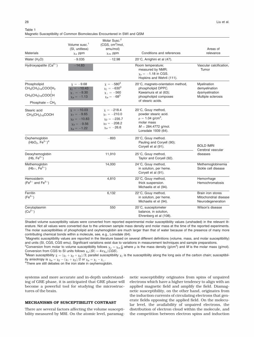
Table 1

Magnetic Susceptibility of Common Biomolecules Encountered in SWI and QSM

Materials

Volume susc.1

(SI, unitless)

xv, ppm

Molar Susc.2

(CGS, cm3/mol,

emu/mol)

xm, ppm Conditions and references

Areas of

relevance

Water (H2O) �9.035 �12.98 20�C, Arrighini et al (47).

Hydroxyapatite (Ca2þ) �14.83 Room temperature;

measured by NMR;

xv ¼ �1.18 in CGS.

Hopkins and Wehrli (111).

Vascular calcification,

Tumor

Phospholipid �x ¼ �9.68 �x ¼ �5803 20�C, magneto-orientation method,

phospholipid DPPC.

Kawamura et al (63);

phospholipid composes

of stearic acids.

Myelination

demyelination

dysmyelination

Multiple sclerosis

CH3(CH2)16COOCjH2

CH3(CH2)16COOCjH

Phosphate – CH2

xk ¼ �10.43

x? ¼ �9.30

xa ¼ �1.13

xk ¼ �6303

x? ¼ �560

xa ¼ �683

Stearic acid

CH3(CH2)16COOH

�x ¼ �10.03

x1 ¼ �9.65

x2 ¼ �10.83

x3 ¼ �9.56

xa ¼ �1.22

�x ¼ �218.4

x1 ¼ �210.0

x2 ¼ �235.7

x3 ¼ �208.2

xa ¼ �26.6

20�C, Gouy method,

powder stearic acid.

r ¼ 1.04 g/cm3,

molar mass

M ¼ 284.4772 g/mol.

Lonsdale 1939 (64).

Oxyhemoglobin

(HbO2, Fe3þ)4�893 20�C, Gouy method.

Pauling and Coryell (90);

Coryell et al (91). BOLD fMRI

Cerebral vascular

diseasesDeoxyhemoglobin

(Hb, Fe2þ)

11,910 25�C, Gouy method,

Taylor and Coryell (92).

Methemoglobin

(Hbþ, Fe3þ)

14,000 24�C, Gouy method,

in solution, per heme.

Coryell et al (91).

Methemoglobinemia

Sickle cell disease

Hemosiderin

(Fe2þ and Fe3þ)

4,810 22�C, Gouy method,

thick suspension.

Michaelis et el (94).

Hemorrhage

Hemochromatosis

Ferritin

(Fe3þ)

6,132 22�C, Gouy method,

in solution, per heme.

Michaelis et el (94).

Brain iron stores

Mitochondrial disease

Neurodegeneration

Ceruloplasmin

(Cu2þ)

550 20�C, susceptometer

balance, in solution,

Ehrenberg et al (108).

Wilson’s disease

Shaded volume susceptibility values were converted from reported experimental molar susceptibility values (unshaded) in the relevant lit-

erature. Not all values were converted due to the unknown sample mass density and molar mass at the time of the reported experiments.

The molar susceptibilities of phospholipid and oxyhemoglobin are much larger than that of water because of the presence of many more

contributing chemical bonds within a molecule, see, e.g., Lonsdale (64).1Magnetic susceptibility values are reported in the literature based on several different definitions (volume, mass, and molar susceptibility)

and units (SI, CGS, CGS emu). Significant variations exist due to variations in measurement techniques and sample preparations.2Conversion from molar to volume susceptibility follows xv ¼ xm

r

M where r is the mass density (g/cm3) and M is the molar mass (g/mol).

Conversion from CGS to SI units follows xv ðSIÞ ¼ 4pxv ðCGSÞ.3Mean susceptibility �x ¼ ðx1 þ x2 þ x3Þ=3; parallel susceptibility xk is the susceptibility along the long axis of the carbon chain; susceptibil-

ity anisotropy is xa ¼ x2 � ðx1 þ x3Þ=2 or xa ¼ xk � x?.4There are still debates on the iron state in oxyhemoglobin.

28 Liu et al.

currents will together determine the molecule’s suscep-tibility and anisotropy. Finally, the microstructure ofthe brain tissue, i.e., the spatial arrangement of mole-cules and organelles within a voxel, will affect themicroscopic magnetic field distribution within thevoxel. As the water molecules are distributed withinthis heterogeneous magnetic field environment, whatMRI phase measures is the averaged effect as seen bythese molecules. As a result, the distribution (e.g.,compartmentalization) and motion of the water mole-cules affect the perceived phase shift. In a healthyadult brain, the most striking feature of phase and sus-ceptibility maps are that the gray matter largelyappears paramagnetic and the white matter largely dia-magnetic (5,9,48). The emerging consensus is that theparamagnetic susceptibility of gray matter is mainlyrelated to iron and the diamagnetic susceptibility ofwhite matter is due to myelination.

Brain Iron

While iron is ferromagnetic and iron is present in thehuman body, no known human tissues are actuallyferromagnetic. In human beings, iron is mostly storedin ferritin and hemosiderin; both are paramagnetic(Table 1). In the brain, certain regions have a prefer-ential accumulation of nonheme iron. Hallgren andSourander (61) studied the distribution of iron ineighty-one brains at autopsy. They found a progres-sive increase in iron distribution that plateaus in thelate teens or twenties with a second, milder increase

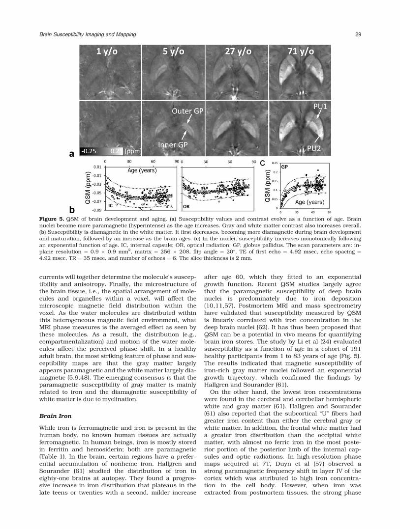
after age 60, which they fitted to an exponentialgrowth function. Recent QSM studies largely agreethat the paramagnetic susceptibility of deep brainnuclei is predominately due to iron deposition(10,11,57). Postmortem MRI and mass spectrometryhave validated that susceptibility measured by QSMis linearly correlated with iron concentration in thedeep brain nuclei (62). It has thus been proposed thatQSM can be a potential in vivo means for quantifyingbrain iron stores. The study by Li et al (24) evaluatedsusceptibility as a function of age in a cohort of 191healthy participants from 1 to 83 years of age (Fig. 5).The results indicated that magnetic susceptibility ofiron-rich gray matter nuclei followed an exponentialgrowth trajectory, which confirmed the findings byHallgren and Sourander (61).

On the other hand, the lowest iron concentrationswere found in the cerebral and cerebellar hemisphericwhite and gray matter (61). Hallgren and Sourander(61) also reported that the subcortical “U” fibers hadgreater iron content than either the cerebral gray orwhite matter. In addition, the frontal white matter hada greater iron distribution than the occipital whitematter, with almost no ferric iron in the most poste-rior portion of the posterior limb of the internal cap-sules and optic radiations. In high-resolution phasemaps acquired at 7T, Duyn et al (57) observed astrong paramagnetic frequency shift in layer IV of thecortex which was attributed to high iron concentra-tion in the cell body. However, when iron wasextracted from postmortem tissues, the strong phase

Figure 5. QSM of brain development and aging. (a) Susceptibility values and contrast evolve as a function of age. Brainnuclei become more paramagnetic (hyperintense) as the age increases. Gray and white matter contrast also increases overall.(b) Susceptibility is diamagnetic in the white matter. It first decreases, becoming more diamagnetic during brain developmentand maturation, followed by an increase as the brain ages. (c) In the nuclei, susceptibility increases monotonically followingan exponential function of age. IC, internal capsule; OR, optical radiation; GP, globus pallidus. The scan parameters are: in-plane resolution ¼ 0.9 � 0.9 mm2, matrix ¼ 256 � 208, flip angle ¼ 20�, TE of first echo ¼ 4.92 msec, echo spacing ¼4.92 msec, TR ¼ 35 msec, and number of echoes ¼ 6. The slice thickness is 2 mm.

Brain Susceptibility Imaging and Mapping 29

and susceptibility contrast between cortical gray andwhite matter did not change significantly (62). This isbecause the susceptibility of the white matter is pre-dominantly determined by myelin.

Myelin

In the phase and susceptibility maps of the brain,white matter consistently shows diamagnetic suscep-tibility. It is now clear that this diamagnetic suscepti-bility is due to the presence of myelin. Myelin is aspiraling sheath that wraps around nerves, includingthose in the brain and spinal cord. It is made up ofproteins and lipids that provide electric insulation.Most proteins and lipids have diamagnetic suscepti-bility. For example, phospholipids have a mean molarsusceptibility of –580 cm3/mol (CGS units) and areanisotropic (Table 1) (63,64). The volume susceptibil-ity of phospholipids is also slightly more diamagneticthan water (Table 1). The purpose of the myelinsheath is to allow action potentials to transmit quicklyand efficiently along the axons of nerve cells. Myelinis essential for the proper functioning of the nervoussystem. Loss of the myelin sheath is the hallmark of anumber of neurodegenerative autoimmune diseasesincluding multiple sclerosis. The importance of myelinin forming the diamagnetism and susceptibility ani-sotropy has been demonstrated in a number of stud-ies. In one study, it was shown that the strongsusceptibility contrast between white and gray matterdisappeared in the transgenic dysmyelinating shiverermouse whose myelin did not develop properly (65).The phase contrast also decreased when mice werefed with a cuprizone diet that resulted in demyelin-ation in the central nervous system (66).

Myelination is also an age-dependent process. Bothhuman and rodent brains are poorly or not myelin-ated at birth. Myelination occurs rapidly in the firstfew years of life for human and in the first few weeksfor rodents. On the other hand, demyelination occursas the brain ages. In human neonates, it was shownthat phase contrast was reduced (67). In the develop-ing mouse brain from postnatal day 4 (PND4) toPND40, it was also observed that phase contrastbetween gray and white matter correlated with theoptical intensity of myelin stained histological slides(68). However, both studies were based on phase con-trast rather than the more intrinsic tissue susceptibil-ity value. In a recent QSM study of 191 participantsfrom 1 to 83 years of age, it was further revealed thatsusceptibility of white matter first became more dia-magnetic as the brain developed, followed by a con-tinuing decrease in diamagnetism as the brain aged(24) (Fig. 5). This developmental trajectory wasexplained by the myelination and demyelination pro-cess which occurred in normal brain developmentand aging. In the mouse brain, Argyridis et al (20)evaluated the temporal evolution of magnetic suscep-tibility in the white matter of mouse C57BL/6 fromPND2 to PND56. They confirmed that susceptibilitybecame increasingly diamagnetic as the brain devel-oped. More interestingly, they also found that suscep-tibility anisotropy increased monotonically as a

function of age; there was a sign change for suscepti-bility in the white matter around the third week, anddiamagnetic susceptibility was highly correlated withmyelin staining intensity (R2 ¼ 0.93).

Microstructure

Besides its chemical and molecular composition,brain tissue’s microstructure (cellular and subcellularstructures and arrangement of cells) also play a cru-cial role in affecting the MRI-measured susceptibility.Compartmentalization of white matter (e.g., separa-tion of axonal space, myelin space, and extracellularspace) plays a significant role in affecting the phaseand T2* signal behavior (18,42,69,70). Protons in eachcompartment experience unique magnetic field andrelaxation properties. The effect of microstructure canbe generalized into two categories: orientation depend-ence and distribution of subvoxel magnetic field.These effects are especially prominent in the whitematter due to its unique microstructure that cannotbe treated as homogeneous even in a statistical sense.

Orientation effects include the angular dependenceof magnetic fields generated by elongated structures(71) and the angular dependence due to underlyinganisotropic susceptibility (35,41). For simplicity, wewill refer to the former as “structural anisotropy” andthe latter as “susceptibility anisotropy.” Structuralanisotropy can generate orientation-dependent phaseeven with only isotropic susceptibility simply due tothe geometric shape. A classic example is the fieldshift of a vessel inside the magnet which is dependenton the relative angle between the vessel and the field(59). In an analysis of gray-white matter phase con-trast, He and Yablonskiy (71) predicted a dependenceof white matter phase on the relative angle betweenaxons and magnetic field due to the elongated shapeof the axons similar to the vessels.

Susceptibility anisotropy describes that magneticsusceptibility is a tensor quantity rather than a scalarquantity (35). As a result, the interaction betweensusceptibility and magnetic field follows the rule oftensor-vector product rather than a simple scalingeffect. In brain tissues, especially in the white matter,this anisotropy originates mainly from membrane lip-ids (37). Each lipid molecule has an anisotropicresponse to an external magnetic field due to itschain-like structure and nonspherical distribution ofelectron clouds. Li et al (37) demonstrated that it wasthe anisotropic susceptibility of lipid molecules andthe ordered arrangement of these lipids that gave riseto the bulk susceptibility anisotropy observed on thevoxel level. Wharton and Bowtell (42) simulated thefield distribution within myelinated axons by model-ing axons as hollow cylinders. They concluded thatanisotropic susceptibility of myelin was needed tofully explain the behavior of the GRE phase.

For a given imaging voxel containing heterogeneousstructures, magnetic field within the voxel is also het-erogeneous, while the total magnetization of the voxelis a summation of all spins within the voxel, eachexperiencing a slightly different local magnetic field.The phase angle of the resulting signal represents the

30 Liu et al.

strength of the mean field. The spatial heterogeneity,however, is lost during the ensemble averaging. Liuand Li proposed a spectral analysis technique in theFourier spectrum space (p-space) that could recoverthe field distribution within the voxel thus allowed

them to infer the underlying tissue microstructure

(60). Specifically, this method measures the spatial

variation of the magnetic field within a voxel that is

induced by the underlying structural heterogeneity.

The underlying principle is that, in the direction par-

allel to the axons, the field variation is expected to be

minimal, while the variation is the largest in the direc-

tions perpendicular to the axons. The ability to detect

such spatial variations is enhanced at higher field

strengths due to the increased susceptibility effect.

Other Sources

There are a number of other sources that affect GREphase contrast in the brain. In the blood pool, oxy-genation changes hemoglobin from being paramag-netic (deoxyhemoglobin) to being diamagnetic

(oxyhemoglobin) (Table 1). This change of magneticproperty is essential for visualizing veins with SWIand is the basic mechanism underlying blood oxygen-ation level-dependent (BOLD) functional MRI (fMRI)(72). However, hemoglobin does not play any signifi-cant role in affecting the susceptibility contrastbetween gray and white matter (73). Chemicalexchange between mobile protons and proteins doesaffect the phase contrast between gray and whitematter and it decreases the susceptibility-inducedcontrast (74).

While the effect of calcium on phase and suscepti-bility contrast in healthy brain tissues has not beenfully investigated, calcification in diseased tissuessuch as tumors causes the local tissue to appear dia-magnetic (16). This shift is the opposite of that causedby iron deposition. Schweser et al (16), for example,used this diamagnetic property to delineate calcifiedlesions, vessels, and potentially iron-laden tissue.They showed that discrimination of para- from dia-magnetic lesions was possible and the results wereconfirmed by the additional computed tomography(CT) in one patient.

Figure 6. An 8-year-old boy with hemorrhage from an ateriovenous malformation. (a) CT obtained at presentation showedright frontal lobe hemorrhage (arrow). (b) QSM obtained at 3T shortly after the CT showed bright signal abnormality, confirm-ing the presence of iron/hemorrhage (arrow). Additional areas of curvilinear and nodular bright signal was seen medial to thelesion, possibly suggesting additional areas of hemorrhage, thromboses, or abnormal vasculature or draining vein containingdeoxyhemoglobin (arrowhead). GRE sequence parameters are: 3D multiecho EPI, flip angle 20�, 1 � 1 � 1 mm3, BW 62.50kHz, TR ¼ 59.3 msec, TE ¼ 13, 28, 43 msec. (c) SWI minIP image demonstrated abnormal vascular tangle typical of arterio-venous malformation (arrow). (d) Final diagnosis of arteriovenous malformation was confirmed by cerebral angiogram.

Brain Susceptibility Imaging and Mapping 31

CLINICAL AND RESEARCH APPLICATIONS

SWI is now commonly used in clinical neuroimaging,while applications of susceptibility mapping techniquesare still primarily in the research stage. Reflecting thecontrast mechanisms outlined in the previous section,the applications of these techniques generally involvechanges of substances in the brain that exhibit differentmagnetic susceptibility compared to the surroundingtissues and structures.

SWI of Cerebral Vascular Pathology

A key application of SWI is aiding the diagnosis of dis-eases involving cerebral vascular pathology. Thesechanges include, for example, vascular malformations(e.g., arteriovenous malformations and cerebral cav-ernous malformations), restrictions in blood flow (e.g.,developmental venous anomaly) and hemorrhages(caused by e.g., cerebral amyloid angiopathy, stroke,and traumatic injuries) (1,3,75–89). In these cases, acommon source of contrast is oxygenation-relatedsusceptibility changes occurring in blood products (3).The main blood oxygen carrier, hemoglobin, containsa heme molecule with an Fe2þ atom. Due to the bind-ing with oxygen, oxyhemoglobin has no unpaired elec-trons; its susceptibility is determined by the proteinshell and thus is diamagnetic (90,91) (Table 1). Deox-yhemoglobin, on the other hand, has four unpaired

electrons per heme and is paramagnetic (90,92) (Table1). Deoxyhemoglobin can be further oxidized to meth-emoglobin (ferrihemoglobin) which contains an Fe3þ

per heme with five unpaired electrons (91) (Table 1).Although methemoglobin has low concentration innormal blood, its concentration increases followinghemorrhage, but the effect is mostly manifested as T1-shortening rather than susceptibility effects (91,93).In the final stages, after hemorrhage, hemosiderinoften forms when macrophages phagocytose anddegrade the extracellular hemoglobin; hemosiderin isalso paramagnetic (94) (Table 1).

Arteriovenous malformations (AVM) is one exampleof vascular malformation which consists of arteriove-nous shunt with branches off the internal carotidartery (ICA) and cerebral veins. Small AVMs may beoccult on CT angiography (CTA) or MRA, yet be readilyidentified on SWI (75). Although small, these AVMs canhemorrhage and thus are not clinically insignificant.Figure 6 illustrates one example of hemorrhage fromAVM in an 8-year-old boy whose positive susceptibilityenhancement can be verified by QSM (Fig. 6b). In addi-tion, effects associated with AVM other than hemor-rhage are also visible on SWI (75,95): for example,intravascular hyperintensity near AVM may suggestoxygenated blood due to rapid arteriovenous shuntingand rapid flow to the varix via the AVM; hyperintensityof parenchyma may suggest edema due to the T2 effectof AVM-related venous hypertension or AVM-relatedsteal phenomenon; on the other hand, hypointensitymay suggest prolonged time passage of normal intra-cranial blood, venous engorgement, or possible func-tional obstruction caused by the AVM.

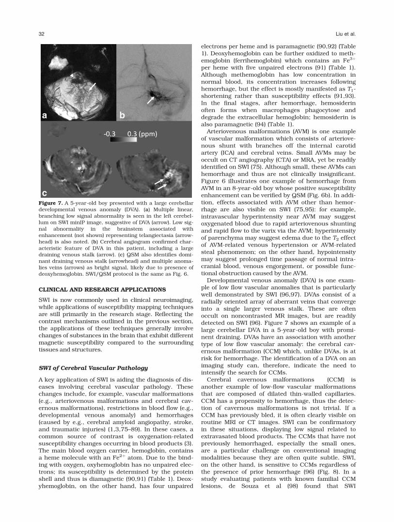
Developmental venous anomaly (DVA) is one exam-ple of low flow vascular anomalies that is particularlywell demonstrated by SWI (96,97). DVAs consist of aradially oriented array of aberrant veins that convergeinto a single larger venous stalk. These are oftenoccult on noncontrasted MR images, but are readilydetected on SWI (96). Figure 7 shows an example of alarge cerebellar DVA in a 5-year-old boy with promi-nent draining. DVAs have an association with anothertype of low flow vascular anomaly: the cerebral cav-ernous malformation (CCM) which, unlike DVAs, is atrisk for hemorrhage. The identification of a DVA on animaging study can, therefore, indicate the need tointensify the search for CCMs.

Cerebral cavernous malformations (CCM) isanother example of low-flow vascular malformationsthat are composed of dilated thin-walled capillaries.CCM has a propensity to hemorrhage, thus the detec-tion of cavernous malformations is not trivial. If aCCM has previously bled, it is often clearly visible onroutine MRI or CT images. SWI can be confirmatoryin these situations, displaying low signal related toextravasated blood products. The CCMs that have notpreviously hemorrhaged, especially the small ones,are a particular challenge on conventional imagingmodalities because they are often quite subtle. SWI,on the other hand, is sensitive to CCMs regardless ofthe presence of prior hemorrhage (96) (Fig. 8). In astudy evaluating patients with known familial CCMlesions, de Souza et al (98) found that SWI

Figure 7. A 5-year-old boy presented with a large cerebellardevelopmental venous anomaly (DVA). (a) Multiple linear,branching low signal abnormality is seen in the left cerebel-lum on SWI minIP image, suggestive of DVA (arrow). Low sig-nal abnormality in the brainstem associated withenhancement (not shown) representing telangiectasia (arrow-head) is also noted. (b) Cerebral angiogram confirmed char-acteristic feature of DVA in this patient, including a largedraining venous stalk (arrow). (c) QSM also identifies domi-nant draining venous stalk (arrowhead) and multiple anoma-lies veins (arrows) as bright signal, likely due to presence ofdeoxyhemoglobin. SWI/QSM protocol is the same as Fig. 6.

32 Liu et al.

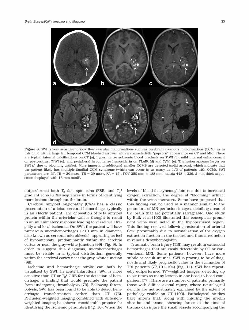
outperformed both T2 fast spin echo (FSE) and T2*gradient echo (GRE) sequences in terms of identifyingmore lesions throughout the brain.

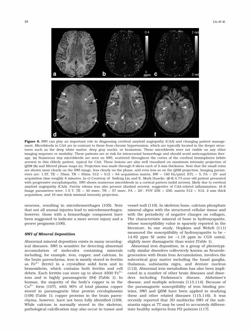
Cerebral Amyloid Angiopathy (CAA) has a classicpresentation of a lobar cerebral hemorrhage, typicallyin an elderly patient. The deposition of beta amyloidprotein within the arteriolar wall is thought to resultin an inflammatory response leading to vessel wall fra-gility and local ischemia. On SWI, the patient will havenumerous microhemorrhages (<10 mm in diameter,also known as cerebral microbleeds), appearing as fociof hypointensity, predominantly within the cerebralcortex or near the gray–white junction (99) (Fig. 9). Inorder to suggest this diagnosis, microhemorrhagesmust be visible in a typical distribution, generallywithin the cerebral cortex near the gray–white junction(99).

Ischemic and hemorrhagic stroke can both bevisualized by SWI. In acute infarctions, SWI is moresensitive than CT or T2* GRE for the detection of hem-orrhage, a finding that would preclude the patientfrom undergoing thrombolysis (79). Following throm-bolysis, SWI has been found to be able to detect hem-orrhagic transformation earlier than CT (76).Perfusion-weighted imaging combined with diffusion-weighted imaging has shown considerable promise foridentifying the ischemic penumbra (Fig. 10). When the

levels of blood deoxyhemoglobin rise due to increasedoxygen extraction, the degree of “blooming” artifactwithin the veins increases. Some have proposed thatthis finding can be used in a manner similar to thepenumbra of MR perfusion images, detailing areas ofthe brain that are potentially salvageable. One studyby Baik et al (100) illustrated this concept, as promi-nent veins were noted in the hypoperfused region.This finding resolved following restoration of arterialflow, presumably due to normalization of the oxygenextraction fraction in the tissues and thus a reductionin venous deoxyhemoglobin.

Traumatic brain injury (TBI) may result in extraaxialhemorrhages that are easily detectable by CT or con-ventional MRI. Some patients, however, have moresubtle or occult injuries. SWI is proving to be of diag-nostic and likely prognostic value in the evaluation ofTBI patients (77,101–104) (Fig. 11). SWI has repeat-edly outperformed T2*-weighted images, detecting upto six times as many lesions in one head-to-head com-parison (77). There are a number of patients, primarilythose with diffuse axonal injury, whose neurologicaldeficits are not adequately explained by the extent ofpathology visible on CT (103). Pathological studieshave shown that, along with injuring the myelinsheaths and axons, shearing forces at the time oftrauma can injure the small vessels accompanying the

Figure 8. SWI is very sensitive to slow flow vascular malformations such as cerebral cavernous malformations (CCM), as inthis child with a large left temporal CCM (dashed arrows), with a characteristic “popcorn” appearance on CT and MRI. Thereare typical internal calcifications on CT (a), hyperintense subacute blood products on T1WI (b), mild internal enhancementon postcontrast T1WI (c), and peripheral hypointense hemosiderin on FLAIR (d) and T2WI (e). The lesion appears larger onSWI (f) due to blooming artifact. More important, additional smaller CCMS are detected (solid arrows), which indicate thatthe patient likely has multiple familial CCM syndrome (which can occur in as many as 1/3 of patients with CCM). SWIparameters are: 3T, TE ¼ 20 msec, TR ¼ 29 msec, FA ¼ 15�, FOV 250 mm � 188 mm, matrix 448 � 336, 2 mm thick acqui-sition displayed with 16 mm minIP.

Brain Susceptibility Imaging and Mapping 33

neurons, resulting in microhemorrhages (105). Notethat not all axonal injuries lead to microhemorrhages;however, those with a hemorrhagic component havebeen suggested to indicate a more severe injury and apoorer prognosis (106).

SWI of Mineral Deposition

Abnormal mineral deposition exists in many neurolog-ical diseases. SWI is sensitive for detecting abnormalaccumulation of molecules containing mineralsincluding, for example, iron, copper, and calcium. Inthe brain parenchyma, iron is mostly stored in ferritinas Fe3þ (ferric) in a crystalline solid form and inhemosiderin, which contains both ferritin and celldebris. Each ferritin can store up to about 4500 Fe3þ

ions and is highly paramagnetic (94) (Table 1). Inhuman, the majority of the body’s copper is in theCu2þ form (107), with 90% of total plasma copperstored in paramagnetic blue protein ceruloplasmin(108) (Table 1); copper proteins in the brain paren-chyma, however, have not been fully identified (109).While calcium is normally stored in the skeleton,pathological calcification may also occur in tumor and

vessel wall (110). In skeleton bone, calcium phosphatemineral aligns with the structured cellular tissue andwith the periodicity of negative charges on collagen.The characteristic mineral of bone is hydroxyapatite,whose susceptibility value is sparsely reported in theliterature. In one study, Hopkins and Wehrli (111)measured the susceptibility of hydroxyapatite to be –14.82 ppm SI units (or –1.18 ppm in CGS units),slightly more diamagnetic than water (Table 1).

Abnormal iron deposition, in a group of phenotypi-cally similar disorders collectively known as Neurode-generation with Brain Iron Accumulation, involves thesubcortical gray matter including the basal ganglia,thalamus, substantia nigra, and dentate nucleus(112). Abnormal iron metabolism has also been impli-cated in a number of other brain diseases and disor-ders including Parkinson’s disease, Alzheimer’sdisease, and multiple sclerosis (113,114). Because ofthe paramagnetic susceptibility of iron binding pro-teins, SWI and QSM have been applied in studyingthese and other related diseases (115,116). It wasrecently reported that 3D multiecho SWI of the sub-stantia nigra at 7T may be used to accurately differen-tiate healthy subjects from PD patients (117).

Figure 9. SWI can play an important role in diagnosing cerebral amyloid angiopathy (CAA) and changing patient manage-ment. Microbleeds in CAA are in contrast to those from chronic hypertension, which are typically located in the deeper struc-tures such as the deep white matter, deep gray nuclei, or brainstem. These microbleeds were not visible on any otherimaging sequence or modality. These patients are at risk for intracranial hemorrhage and should avoid anticoagulation ther-apy. (a) Numerous tiny microbleeds are seen on SWI, scattered throughout the cortex of the cerebral hemispheres (whitearrows) in this elderly patient, typical for CAA. These lesions are also well visualized on maximum intensity projection ofQSM (b) and filtered phase maps (c). Projection was made through 8 slices each of 2-mm thickness. Note that the small veinsare shown most clearly on the SWI image, less clearly on the phase, and even less so on the QSM projection. Imaging param-eters are: 1.5T, TE ¼ 35ms, TR ¼ 85ms, 512 � 512 � 64 acquisition matrix, BW ¼ 160 Hz/pixel, ETL ¼ 5, FA ¼ 25� andacquisition time roughly 8 minutes. (a–c) Courtesy of Saifeng Liu and E. Mark Haacke. (d–f) A 73-year-old patient presentedwith progressive encephalopathy. SWI shows numerous microbleeds in a cortical pattern (solid arrows), likely due to cerebralamyloid angiopathy (CAA). Patchy edema was also present (dashed arrows), suggestive of CAA-related inflammation. (d–f)Image parameters were: 1.5 T, TE ¼ 40 msec, TR ¼ 57 msec, FA ¼ 20�, FOV 256 � 256, matrix 512 � 512, 2 mm thickacquisition, and 16 mm thick minimal intensity projection.

34 Liu et al.

Wilson’s disease (WD), on the other hand, is dueto an abnormality in copper metabolism with theend result being excessive copper accumulation,particularly in the subcortical gray matter struc-tures (globus pallidus, putamen, thalamus, dentatenucleus, pons, and midbrain) (118). In a study with23 WD subjects and 23 controls, Bai et al (119)found significant negative phase values in the sub-cortical gray matter. Fritzsch et al (120), using QSM,showed that patients with WD had significantlyincreased susceptibility in all analyzed basal gangliaregions compared with healthy controls, which wasevident not only in patients with a neurological syn-drome but also in patients with isolated hepaticmanifestations.

Applications of Susceptibility Mapping

Although the diagnostic value of QSM still needs to befully investigated, the quantitative information hasalready shed additional light on brain development,aging, and the evolution of pathologies. One immedi-ate potential clinical utility of QSM is to improve thelocalization and quantification of calcium with MRI,which can be differentiated from microbleeds and irondeposition due to the diamagnetic nature of calcifica-tion (Table 1) (16) (Fig. 12). In one study, QSM pro-vided more accurate differentiation of calcificationsfrom hemorrhage (21). One benefit of establishing anMRI-based method for detecting calcification is toreduce radiation exposure to vulnerable pediatricpatients.

In multiple sclerosis (MS) patients, SWI allows thevisualization of the anatomic relationship of the demye-linating plaque and the penetrating veins (121,122). Inone study, combining conventional imaging sequenceswith SWI demonstrated �50% more lesions than didthe conventional sequences alone, including those inthe cortical gray matter that were often difficult to

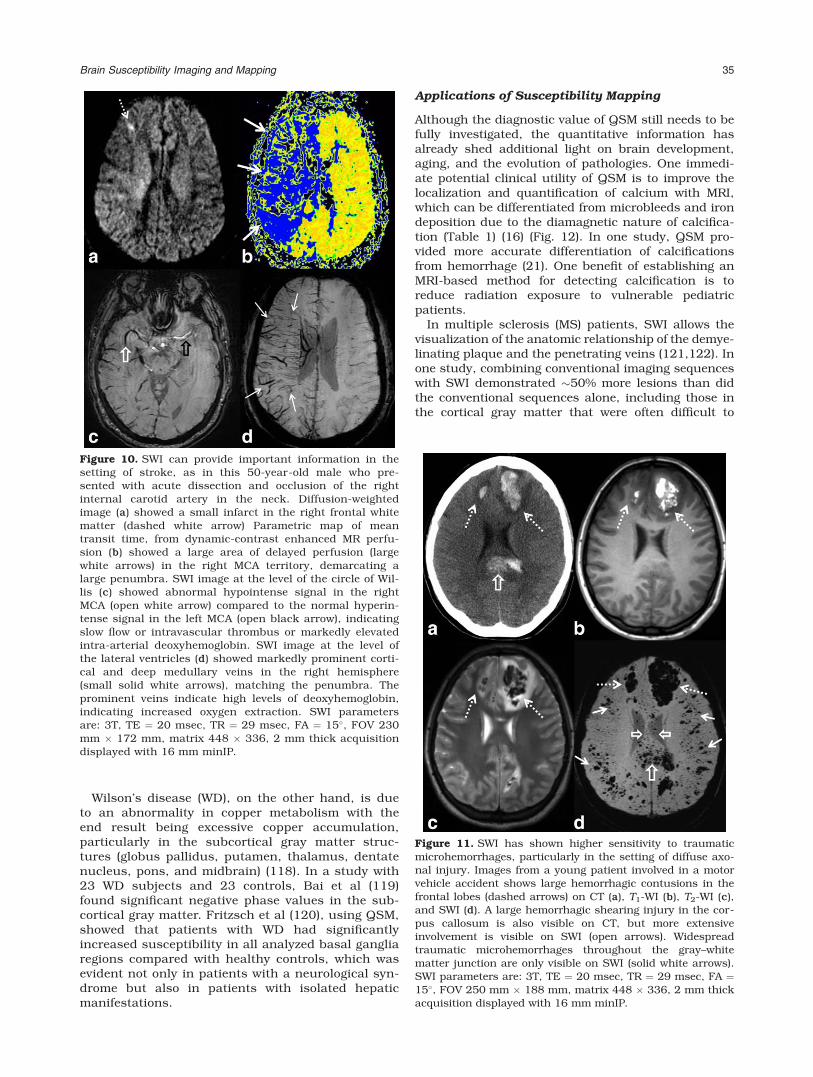
Figure 10. SWI can provide important information in thesetting of stroke, as in this 50-year-old male who pre-sented with acute dissection and occlusion of the rightinternal carotid artery in the neck. Diffusion-weightedimage (a) showed a small infarct in the right frontal whitematter (dashed white arrow) Parametric map of meantransit time, from dynamic-contrast enhanced MR perfu-sion (b) showed a large area of delayed perfusion (largewhite arrows) in the right MCA territory, demarcating alarge penumbra. SWI image at the level of the circle of Wil-lis (c) showed abnormal hypointense signal in the rightMCA (open white arrow) compared to the normal hyperin-tense signal in the left MCA (open black arrow), indicatingslow flow or intravascular thrombus or markedly elevatedintra-arterial deoxyhemoglobin. SWI image at the level ofthe lateral ventricles (d) showed markedly prominent corti-cal and deep medullary veins in the right hemisphere(small solid white arrows), matching the penumbra. Theprominent veins indicate high levels of deoxyhemoglobin,indicating increased oxygen extraction. SWI parametersare: 3T, TE ¼ 20 msec, TR ¼ 29 msec, FA ¼ 15�, FOV 230mm � 172 mm, matrix 448 � 336, 2 mm thick acquisitiondisplayed with 16 mm minIP.

Figure 11. SWI has shown higher sensitivity to traumaticmicrohemorrhages, particularly in the setting of diffuse axo-nal injury. Images from a young patient involved in a motorvehicle accident shows large hemorrhagic contusions in thefrontal lobes (dashed arrows) on CT (a), T1-WI (b), T2-WI (c),and SWI (d). A large hemorrhagic shearing injury in the cor-pus callosum is also visible on CT, but more extensiveinvolvement is visible on SWI (open arrows). Widespreadtraumatic microhemorrhages throughout the gray–whitematter junction are only visible on SWI (solid white arrows).SWI parameters are: 3T, TE ¼ 20 msec, TR ¼ 29 msec, FA ¼15�, FOV 250 mm � 188 mm, matrix 448 � 336, 2 mm thickacquisition displayed with 16 mm minIP.

Brain Susceptibility Imaging and Mapping 35

visualize on fluid-attenuated inversion recovery (FLAIR)(115). While demyelination is the hallmark of MS, ele-vated iron deposits have also been reported in MSbrains (123,124). Both demyelination and iron deposi-tion increase local tissue susceptibility which can bequantified by QSM (Fig. 13), although differentiatingtheir relative contributions remains a topic of research.It has been shown that loss of myelin causes the sus-ceptibility of white matter to increase (i.e., becomingless diamagnetic), approaching that of gray matter(65,66). At the same time, demyelination reduces R2*while iron deposition increases R2*. These competingeffects on R2* have been thought to result in theimproved sensitivity of QSM over R2* in evaluatingchanges in the basal ganglia of MS patients (22). Fur-ther, QSM of MS lesions at various ages showed thatlesions’ susceptibility increased rapidly as it changedfrom being enhanced to nonenhanced; during the firstfew years, lesions attained a high susceptibility valueand gradually dissipated back to susceptibility similarto that of normal-appearing white matter as the lesionsaged (34).

The quantitative nature of QSM offers an opportunityto correlate susceptibility values with clinical condi-tions and treatment outcomes. In a recent study of b-thalassemia, a blood disorder that reduces the produc-tion of hemoglobin, in 31 patients who had been under

blood transfusion treatment, 27 (87.1%) had abnormaliron deposition in one of the regions of interest (ROIs)examined. Compared with healthy control subjects,patients with thalassemia showed significantly lowersusceptibility value in the globus pallidus and sub-stantia nigra but significantly higher susceptibilityvalue in the red nucleus and choroid plexus (125).QSM should also be relevant for evaluating the effect ofchelation on brain iron in other diseases such as sicklecell disease and Parkinson’s disease.

QSM is also being applied to quantify cerebral perfu-sion, as susceptibility changes in the blood can bedirectly related to the concentration of gadolinium-based contrast agent (33) or endogenous deoxyhemo-globin (126,127). The theoretical advantage of QSM asopposed to T2*-weighted images is to provide a moreaccurate estimate of tissue perfusion without sufferingfrom “blooming” artifacts. Because of its sensitivity todeoxyhemoglobin, QSM allows the mapping of thesource of the BOLD contrast in gradient echo fMRI(128,129). In one recent study at 7T, it was reportedthat the sensitivity and spatial reliability of functionalQSM relative to the magnitude data depended stronglyon the significance threshold that defines “activated”voxels in the SPM software, and on the efficiency ofspatiotemporal filtering of the phase time-series (32).For high-resolution 7T data, the observed phase and

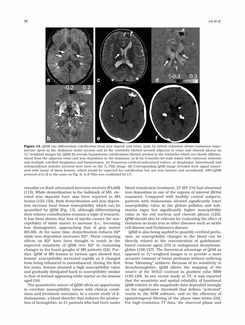
Figure 12. QSM can differentiate calcification from iron deposit and veins. (a,b) An elderly volunteer shows numerous hypo-intense spots in the thalamus (solid arrows) and in the ventricles (dotted arrows) adjacent to veins and choroid plexus onT2*-weighted images (a). QSM (b) reveals hypointense calcifications (dotted arrows) in the ventricles which are clearly differen-tiated from the adjacent veins and iron deposition in the thalamus. (c–f) An 8-month-old male infant with tuberous sclerosisand multiple calcified dysplasias and hamartomas. (c) Numerous cortical/subcortical tubers, or dysplasias, (arrowhead) andsubependymal nodules (arrows) were seen on the T2 FSE image. (d) Corresponding QSM image revealed dark signal associ-ated with many of these lesions, which would be expected for calcification but not iron (arrows and arrowhead). SWI/QSMprotocol of (c,d) is the same as Fig. 6. (e,f) This was confirmed by CT.

36 Liu et al.

susceptibility changes in the cortex have been attrib-uted to blood volume and oxygenation changes in pialand intracortical veins (129).

STI is being developed as a high-resolution fiber-tracking technique. Its feasibility has been demon-strated on mouse brains (38). Improved tracing ofrenal tubules has been recently demonstrated withSTI and it was shown that STI was able to tracktubules throughout the kidney, whereas DTI was lim-ited to the inner medulla in mouse kidneys (40). Fur-ther developments are underway for applications inhuman brains (36,39,43). There is growing evidencesuggesting that QSM and susceptibility anisotropymay be a sensitive measure for loss of myelin in brainwhite matter (20,65,66,68,130). Cao et al (130)

recently reported that prenatal alcohol exposure sig-nificantly reduces susceptibility contrast and suscep-tibility anisotropy of the brain white matter, andmagnetic susceptibility may be more sensitive thanDTI for detecting subtle myelination changes.

IMPLEMENTATIONS AND UNMET NEEDS

Technical Considerations

Most, if not all, modern MRI scanners are readilyequipped with some versions of the 2D and 3D gradientecho sequence. This type of sequence is known to befast, robust, and of low specific absorption rate (SAR). At3T, a typical scan duration is around 5–10 minutes,

Table 2

Examples of SWI and QSM Protocols for the Brain

Field Recon Resolution (mm3) Flip angle TE1 (msec) TR (msec) # echo

1.5 T SWI 0.8 � 0.8 � 2 20� 40 50 1

QSM 0.8 � 0.8 � 2 30� Min 58 Multi

3.0 T SWI 0.8 � 0.8 � 2 15� 20 28 1

QSM 0.8 � 0.8 � 2 12� Min 40 Multi

7.0 T SWI 0.3 � 0.3 � 1.2 15� 15 28 1

QSM 0.8 � 0.8 � 0.8 8� Min 34 Multi

These sequence parameters are not intended as general “recommendations.” Rather, they serve to illustrate parameter examples that

produce good SWI and QSM results. The parameters should be modified for different purposes; for example, multiple echoes can also be

acquired for SWI.

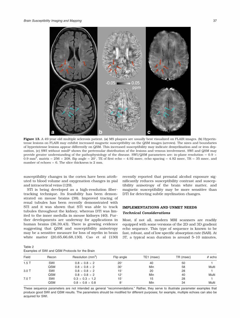
Figure 13. A 49-year-old multiple sclerosis patient. (a) MS plaques are usually best visualized on FLAIR images. (b) Hyperin-tense lesions on FLAIR may exhibit increased magnetic susceptibility on the QSM images (arrows). The sizes and boundariesof hyperintense lesions appear differently on QSM. This increased susceptibility may indicate demyelination and or iron dep-osition. (c) SWI without minIP shows the perivenular distribution of the lesions and venous involvement. SWI and QSM mayprovide greater understanding of the pathophysiology of the disease. SWI/QSM parameters are: in-plane resolution ¼ 0.9 �0.9 mm2, matrix ¼ 256 � 208, flip angle ¼ 20�, TE of first echo ¼ 4.92 msec, echo spacing ¼ 4.92 msec, TR ¼ 35 msec, andnumber of echoes ¼ 6. The slice thickness is 2 mm.

Brain Susceptibility Imaging and Mapping 37

depending on the spatial resolution and slice coverage.The sequence can be optimized with respect to fieldstrength, flip angle, TE, TR, and the tissue and pathol-ogy of interest (Table 2). A key requirement duringacquisition is to store the complex images (both magni-tude and phase) rather than only the magnitude. ForQSM, the orientation of the B0 field needs to be knownwith respect to the imaging matrix.

SNR

A “rule of thumb” for SNR consideration is that opti-mal phase SNR is attained at TE ¼ T2* for a giventype of tissue (131). If the primary purpose is to visu-alize veins and hemorrhages such as in SWI venogra-phy, the TE can be chosen to be around 20 msec at3T; if the purpose is to visualize gray and white mat-ter contrast with QSM, better SNR is achieved withthe TE around 30–40 msec at 3T. Both SWI and QSMbenefit from increasing field strength, as phase accu-mulates faster at higher field, allowing shorter TE andTR, thus less T2* decay, higher SNR, and more rapidacquisition.

Contrast

Since SWI combines both magnitude and phase, con-trast in the magnitude image affects the appearanceof SWI (1). For example, low flip angles and intermedi-ate TEs result in low gray matter and white mattercontrast; a slightly higher flip angle partially sup-presses the cerebrospinal fluid (CSF) and adds someT1-weighting. QSM, on the other hand, is not sensitiveto magnitude contrast except for the potential multi-compartment effect, where relative contributions fromdifferent compartments may vary depending onsequence parameters.

2D vs. 3D

While SWI can be reconstructed from both 2D and 3Ddata, susceptibility mapping is best accomplishedwith a 3D sequence to avoid phase inconsistencyamong adjacent slices, although 2D data are alsocompatible with QSM (32,132). For 2D acquisition, asingle echo with interleaving slices allows fast volumecoverage, which is beneficial for dynamic scans suchas perfusion and functional QSM. For 3D acquisi-tions, multiple echoes offer the flexibility of optimizingSWI contrast (133,134) and improving SNR for QSMthrough multiecho averaging (131). Fast acquisitioncan also be achieved with spiral or EPI trajectories forboth 2D and 3D acquisitions (131,132).

High readout bandwidth (> 62 kHz) and high spa-tial resolution are beneficial for QSM in reducingintravoxel dephasing and subsequent signal loss.Finally, flow compensation is useful for suppressingphase accumulation due to arterial blood and bulkmotion (62,127,135).

For image reconstruction, some MRI manufacturersprovide commercial software to generate SWI imageson the scanner. There are also shared research soft-ware packages now available for susceptibility map-ping (12,23).

Unmet Needs and Future Directions

A growing number of algorithms have been proposedfor QSM, most of which are developed based on lim-ited simulation, phantom, and in vivo data. There is alack of systematic evaluation and critical comparisonsof the accuracy, intersubject variability, and intrasub-ject reproducibility. A rigorous assessment of the per-formances of the algorithms and the dependence onpulse sequences can potentially lead to an acceptablestandard for MRI susceptibility mapping and facilitateits clinical translation. Such an assessment shouldinclude sequence parameters, phase unwrapping,background phase removal, and susceptibility inver-sion algorithms. Establishing such a standard willrequire concerted efforts across multiple centers anddifferent vendors.

A critical obstacle in interpreting susceptibility val-ues is the competing effects of multiple signal sour-ces. While the susceptibility of white matter ispredominantly determined by myelin concentration,iron is also present, e.g., in oligodendrocyte thatforms the myelin and in mitochondria in the axons(136). On the other hand, while the susceptibility ofdeep brain nuclei is mostly determined by iron depo-sition, axons within these nuclei are also myelinated,although to a lesser degree. In pathological tissuessuch as MS plaques, demyelination and iron deposi-tion may coexist. In Wilson’s disease, copper deposi-tion may also be accompanied by iron accumulation(137). While QSM provides a quantification of the sus-ceptibility values, it is unable to differentiate thesediverse sources of susceptibility by itself. Patient his-tory, clinical symptoms, other MRI parameters,sophisticated signal models, and possibly other imag-ing modalities are thus needed to pinpoint the exactcause of detected alterations in susceptibility.

Characterizing and imaging subvoxel magnetic fielddistribution is another emerging area of interest,which may provide insight into tissue microstructure.The volume susceptibility measured by QSM reflectsonly the mean field shift of a given voxel, it does notportray the field heterogeneity within the voxel. Abasic model for this field heterogeneity is the three-pool model of axonal water, myelin water, and extrac-ellular water (42,69). A more systematic way to extractthe subvoxel field information is to perform a Fourierspectral analysis with the p-space technique whichhas been demonstrated in phantoms and mousebrains ex vivo (60). Another way is to measure diffu-sion attenuation caused by this internal heterogene-ous magnetic field (138,139).

In conclusion, While susceptibility is a major sourceof image artifacts in MRI, technological advances havealso transformed it into a useful source of imagecontrast. SWI is gaining wider acceptance in clinicalpractice. Susceptibility mapping techniques aim toquantify the underlying sources. However, it isacknowledged that QSM provides only a “relative”quantification of susceptibility rather than the abso-lute physical quantity. This is because MRI phase andfrequency values are relative and are also affected byphase filtering procedures, and there is a lack of

38 Liu et al.

universal and reliable frequency reference for in vivoimaging. The clinical application of susceptibilitymapping is still in the early stage of evaluation. Theimmediate goals are to image and quantify many bio-logically and pathologically relevant endogenous mole-cules, exogenous contrast agents, and tissuemicrostructures and their relationships with diseasediagnosis and prognosis.

ACKNOWLEDGMENT

The authors thank E. Mark Haacke, PhD, for com-ments on the article.

REFERENCES

1. Haacke EM, Xu Y, Cheng YC, Reichenbach JR. Susceptibilityweighted imaging (SWI). Magn Reson Med 2004;52:612–618.

2. de Crespigny AJ, Roberts TP, Kucharcyzk J, Moseley ME.Improved sensitivity to magnetic susceptibility contrast. MagnReson Med 1993;30:135–137.

3. Reichenbach JR, Venkatesan R, Schillinger DJ, Kido DK, HaackeEM. Small vessels in the human brain: MR venography withdeoxyhemoglobin as an intrinsic contrast agent. Radiology 1997;204:272–277.

4. de Rochefort L, Brown R, Prince MR, Wang Y. Quantitative MRsusceptibility mapping using piece-wise constant regularizedinversion of the magnetic field. Magn Reson Med 2008;60:1003–1009.

5. Shmueli K, de Zwart JA, van Gelderen P, Li TQ, Dodd SJ, DuynJH. Magnetic susceptibility mapping of brain tissue in vivo usingMRI phase data. Magn Reson Med 2009;62:1510–1522.

6. Young IR, Khenia S, Thomas DG, et al. Clinical magnetic suscepti-bility mapping of the brain. J Comput Assist Tomogr 1987;11:2–6.

7. Weisskoff RM, Kiihne S. MRI susceptometry: image-based mea-surement of absolute susceptibility of MR contrast agents andhuman blood. Magn Reson Med 1992;24:375–383.

8. Li L. Magnetic susceptibility quantification for arbitrarily shapedobjects in inhomogeneous fields. Magn Reson Med 2001;46:907–916.

9. Li W, Wu B, Liu C. Quantitative susceptibility mapping ofhuman brain reflects spatial variation in tissue composition.Neuroimage 2011;55:1645–1656.

10. Bilgic B, Pfefferbaum A, Rohlfing T, Sullivan EV, AdalsteinssonE. MRI estimates of brain iron concentration in normal agingusing quantitative susceptibility mapping. Neuroimage 2012;59:2625–2635.

11. Wu B, Li W, Guidon A, Liu C. Whole brain susceptibility mappingusing compressed sensing. Magn Reson Med 2012;67:137–147.

12. Liu J, Liu T, de Rochefort L, et al. Morphology enabled dipoleinversion for quantitative susceptibility mapping using struc-tural consistency between the magnitude image and the suscep-tibility map. Neuroimage 2012;59:2560–2568.

13. Marques JP, Bowtell R. Application of a Fourier-based methodfor rapid calculation of field inhomogeneity due to spatial varia-tion of magnetic susceptibility. Concept Magn Reson B 2005;25B:65–78.

14. Salomir R DSB, Moonen CTW. A fast calculation method for mag-netic field inhomogeneity due to an arbitrary distribution of bulksusceptibility. Concepts Magn Reson Part B 2003;19B:26–34.

15. Wharton S, Bowtell R. Whole-brain susceptibility mapping athigh field: a comparison of multiple- and single-orientationmethods. Neuroimage 2010;53:515–525.

16. Schweser F, Deistung A, Lehr BW, Reichenbach JR. Differentia-tion between diamagnetic and paramagnetic cerebral lesionsbased on magnetic susceptibility mapping. Med Phys 2010;37:5165–5178.

17. Tang J, Liu S, Neelavalli J, Cheng YCN, Buch S, Haacke EM.Improving susceptibility mapping using a threshold-based k-space/image domain iterative reconstruction approach. MagnReson Med 2013;69:1396–1407.

18. Dibb R, Li W, Cofer W, Liu C. Microstructural origins ofgadolinium-enhanced susceptibility contrast and anisotropy.Magn Reson Med 2014 [Epub ahead of print].

19. Acosta-Cabronero J, Williams GB, Cardenas-Blanco A,Arnold RJ, Lupson V, Nestor PJ. In vivo quantitative susceptibil-ity mapping (QSM) in Alzheimer’s disease. PLoS One 2013;8:e81093.

20. Argyridis I, Li W, Johnson GA, Liu C. Quantitative magnetic sus-ceptibility of the developing mouse brain reveals microstructuralchanges in the white matter. Neuroimage 2013 [Epub ahead ofprint].

21. Deistung A, Schweser F, Wiestler B, et al. Quantitative suscepti-bility mapping differentiates between blood depositions and cal-cifications in patients with glioblastoma. PLoS One 2013;8:e57924.

22. Langkammer C, Liu T, Khalil M, et al. Quantitative susceptibilitymapping in multiple sclerosis. Radiology 2013;267:551–559.

23. Li W, Avram AV, Wu B, Xiao X, Liu C. Integrated Laplacian-based phase unwrapping and background phase removal forquantitative susceptibility mapping. NMR Biomed 2013 [Epubahead of print].

24. Li W, Wu B, Batrachenko A, et al. Differential developmental tra-jectories of magnetic susceptibility in human brain gray andwhite matter over the lifespan. Hum Brain Mapp 2013 [Epubahead of print].

25. Lim IA, Faria AV, Li X, et al. Human brain atlas for automatedregion of interest selection in quantitative susceptibility map-ping: application to determine iron content in deep gray matterstructures. Neuroimage 2013;82C:449–469.

26. Liu T, Wisnieff C, Lou M, Chen W, Spincemaille P, Wang Y. Non-linear formulation of the magnetic field to source relationshipfor robust quantitative susceptibility mapping. Magn Reson Med2013;69:467–476.

27. Schweser F, Deistung A, Sommer K, Reichenbach JR. Towardonline reconstruction of quantitative susceptibility maps: super-fast dipole inversion. Magn Reson Med 2013;69:1582–1594.

28. Sun H, Wilman AH. Background field removal using sphericalmean value filtering and Tikhonov regularization. Magn ResonMed 2013 [Epub ahead of print].

29. Wang S, Lou M, Liu T, Cui D, Chen X, Wang Y. Hematoma vol-ume measurement in gradient echo MRI using quantitative sus-ceptibility mapping. Stroke 2013;44:2315–2317.

30. Xie L, Sparks MA, Li W, et al. Quantitative susceptibility map-ping of kidney inflammation and fibrosis in type 1 angiotensinreceptor-deficient mice. NMR Biomed 2013;26:1853–1863.

31. Zheng W, Nichol H, Liu S, Cheng YC, Haacke EM. Measuringiron in the brain using quantitative susceptibility mapping andX-ray fluorescence imaging. Neuroimage 2013;78:68–74.

32. Balla DZ, Sanchez-Panchuelo RM, Wharton SJ, et al. Functionalquantitative susceptibility mapping (fQSM). Neuroimage 2014;100:112–124.

33. Bonekamp D, Barker PB, Leigh R, van Zijl PC, Li X. Susceptibil-ity-based analysis of dynamic gadolinium bolus perfusion MRI.Magn Reson Med 2014 [Epub ahead of print].

34. Chen W, Gauthier SA, Gupta A, et al. Quantitative susceptibilitymapping of multiple sclerosis lesions at various ages. Radiology2014;271:183–192.

35. Liu C. Susceptibility tensor imaging. Magn Reson Med 2010;63:1471–1477.

36. Li X, Vikram DS, Lim IA, Jones CK, Farrell JA, van Zijl PC. Map-ping magnetic susceptibility anisotropies of white matter in vivoin the human brain at 7 T. Neuroimage 2012;62:314–330.

37. Li W, Wu B, Avram AV, Liu C. Magnetic susceptibility anisotropyof human brain in vivo and its molecular underpinnings. Neuro-image 2012;59:2088–2097.

38. Liu C, Li W, Wu B, Jiang Y, Johnson GA. 3D fiber tractographywith susceptibility tensor imaging. Neuroimage 2012;59:1290–1298.

39. Wisnieff C, Liu T, Spincemaille P, Wang S, Zhou D, Wang Y.Magnetic susceptibility anisotropy: cylindrical symmetry frommacroscopically ordered anisotropic molecules and accuracy ofMRI measurements using few orientations. Neuroimage 2013;70:363–376.

40. Xie L, Dibb R, Cofer GP, et al. Susceptibility tensor imaging ofthe kidney and its microstructural underpinnings. Magn ResonMed 2014 [Epub ahead of print].

Brain Susceptibility Imaging and Mapping 39

41. Lee J, Shmueli K, Fukunaga M, et al. Sensitivity of MRI reso-nance frequency to the orientation of brain tissue microstruc-ture. Proc Natl Acad Sci U S A 2010;107:5130–5135.

42. Wharton S, Bowtell R. Fiber orientation-dependent white mattercontrast in gradient echo MRI. Proc Natl Acad Sci U S A 2012;109:18559–18564.

43. Li X, van Zijl PC. Mean magnetic susceptibility regularized sus-ceptibility tensor imaging (MMSR-STI) for estimating orientationsof white matter fibers in human brain. Magn Reson Med 2014;72:610–619.

44. Sukstanskii AL, Yablonskiy DA. On the role of neuronal mag-netic susceptibility and structure symmetry on gradient echoMR signal formation. Magn Reson Med 2014;71:345–353.

45. Li W, Liu C. Comparison of magnetic susceptibility tensor anddiffusion tensor of the brain. J Neurosci Neuroeng 2013;2:431–440.

46. Liu C, Murphy NE, Li W. Probing white-matter microstructurewith higher-order diffusion tensors and susceptibility tensorMRI. Front Integr Neurosci 2013;7:11.

47. Arrighin GP, Maestro M, Moccia R. Magnetic properties of polya-tomic molecules. I. Magnetic susceptibility of H2o,Nh3, Ch4,H2o2. J Chem Phys 1968;49:882.

48. Schweser F, Deistung A, Lehr BW, Reichenbach JR. Quantitativeimaging of intrinsic magnetic tissue properties using MRI signalphase: an approach to in vivo brain iron metabolism? Neuro-image 2011;54:2789–2807.

49. Cullity BD, Graham CD. Introduction to magnetic materials.Hoboken, NJ: IEEE/Wiley; 2009.

50. Levitt MH. The signs of frequencies and phases in NMR. J MagnReson 1997;126:164–182.

51. Abdul-Rahman HS, Gdeisat MA, Burton DR, Lalor MJ, Lilley F,Moore CJ. Fast and robust three-dimensional best path phaseunwrapping algorithm. Appl Opt 2007;46:6623–6635.

52. Jenkinson M. Fast, automated, N-dimensional phase-unwrap-ping algorithm. Magn Reson Med 2003;49:193–197.

53. Liu T, Khalidov I, de Rochefort L, et al. A novel background fieldremoval method for MRI using projection onto dipole fields(PDF). NMR Biomed 2011;24:1129–1136.

54. Glover GH. Multipoint Dixon technique for water and fat proton andsusceptibility imaging. J Magn Reson Imaging 1991;1:521–530.

55. Conturo TE, Barker PB, Mathews VP, Monsein LH, Bryan RN.MR imaging of cerebral perfusion by phase-angle reconstructionof bolus paramagnetic-induced frequency shifts. Magn ResonMed 1992;27:375–390.

56. Rauscher A, Sedlacik J, Barth M, Mentzel HJ, Reichenbach JR.Magnetic susceptibility-weighted MR phase imaging of thehuman brain. AJNR Am J Neuroradiol 2005;26:736–742.

57. Duyn JH, van Gelderen P, Li TQ, de Zwart JA, Koretsky AP,Fukunaga M. High-field MRI of brain cortical substructure basedon signal phase. Proc Natl Acad Sci U S A 2007;104:11796–11801.

58. Cho ZH, Ro YM, Lim TH. NMR venography using the susceptibil-ity effect produced by deoxyhemoglobin. Magn Reson Med 1992;28:25–38.

59. Yablonskiy DA, Haacke EM. Theory of NMR signal behavior inmagnetically inhomogeneous tissues — the static dephasingregime. Magn Reson Med 1994;32:749–763.

60. Liu C, Li W. Imaging neural architecture of the brain based onits multipole magnetic response. Neuroimage 2013;67:193–202.

61. Hallgren B, Sourander P. The effect of age on the non-haeminiron in the human brain. J Neurochem 1958;3:41–51.

62. Langkammer C, Schweser F, Krebs N, et al. Quantitative suscep-tibility mapping (QSM) as a means to measure brain iron? Apost mortem validation study. Neuroimage 2012;62:1593–1599.

63. Kawamura Y, Sakurai I, Ikegami A, Iwayanagi S. Magneto-orien-tation of phospholipids. Mol Cryst Liq Cryst 1981;67:733–743.

64. Lonsdale K. Diamagnetic anisotropy of organic molecules. ProcR Soc Lond Ser A 1939;171:0541–0568.

65. Liu C, Li W, Johnson GA, Wu B. High-field (9.4 T) MRI of braindysmyelination by quantitative mapping of magnetic susceptibil-ity. Neuroimage 2011;56:930–938.

66. Lee J, Shmueli K, Kang BT, et al. The contribution of myelin tomagnetic susceptibility-weighted contrasts in high-field MRI ofthe brain. Neuroimage 2012;59:3967–3975.

67. Zhong K, Ernst T, Buchthal S, Speck O, Anderson L, Chang L.Phase contrast imaging in neonates. Neuroimage 2011;55:1068–1072.

68. Lodygensky GA, Marques JP, Maddage R, et al. In vivo assess-ment of myelination by phase imaging at high magnetic field.Neuroimage 2012;59:1979–1987.

69. van Gelderen P, de Zwart JA, Lee J, Sati P, Reich DS, Duyn JH.Nonexponential T(2) decay in white matter. Magn Reson Med2012;67:110–117.

70. Chen WC, Foxley S, Miller KL. Detecting microstructural proper-ties of white matter based on compartmentalization of magneticsusceptibility. Neuroimage 2013;70:1–9.

71. He X, Yablonskiy DA. Biophysical mechanisms of phase contrastin gradient echo MRI. Proc Natl Acad Sci U S A 2009;106:13558–13563.

72. Ogawa S, Lee TM, Kay AR, Tank DW. Brain magnetic-resonance-imaging with contrast dependent on blood oxygenation. ProcNatl Acad Sci U S A 1990;87:9868–9872.

73. Lee J, Hirano Y, Fukunaga M, Silva AC, Duyn JH. On the contri-bution of deoxy-hemoglobin to MRI gray-white matter phasecontrast at high field. Neuroimage 2010;49:193–198.

74. Zhong K, Leupold J, von Elverfeldt D, Speck O. The molecularbasis for gray and white matter contrast in phase imaging. Neu-roimage 2008;40:1561–1566.

75. Essig M, Reichenbach JR, Schad LR, Schoenberg SO, Debus J,Kaiser WA. High-resolution MR venography of cerebralarteriovenous malformations. Magn Reson Imaging 1999;17:1417–1425.

76. Hermier M, Nighoghossian N, Derex L, et al. MRI of acute post-ischemic cerebral hemorrhage in stroke patients: diagnosis withT2*-weighted gradient-echo sequences. Neuroradiology 2001;43:809–815.

77. Tong KA, Ashwal S, Holshouser BA, et al. Hemorrhagic shearinglesions in children and adolescents with posttraumatic diffuseaxonal injury: improved detection and initial results. Radiology2003;227:332–339.

78. Tong KA, Ashwal S, Holshouser BA, et al. Diffuse axonal injuryin children: clinical correlation with hemorrhagic lesions. AnnNeurol 2004;56:36–50.

79. Wycliffe ND, Choe J, Holshouser B, Oyoyo UE, Haacke EM, KidoDK. Reliability in detection of hemorrhage in acute stroke by anew three-dimensional gradient recalled echo susceptibility-weighted imaging technique compared to computed tomography:a retrospective study. J Magn Reson Imaging 2004;20:372–377.

80. Choi JH, Mohr JP. Brain arteriovenous malformations in adults.Lancet Neurol 2005;4:299–308.

81. Idbaih A, Boukobza M, Crassard I, Porcher R, Bousser MG,Chabriat H. MRI of clot in cerebral venous thrombosis: highdiagnostic value of susceptibility-weighted images. Stroke 2006;37:991–995.

82. Jeon SB, Kang DW, Cho AH, et al. Initial microbleeds at MRimaging can predict recurrent intracerebral hemorrhage.J Neurol 2007;254:508–512.

83. Chastain CA, Oyoyo UE, Zipperman M, et al. Predicting out-comes of traumatic brain injury by imaging modality and injurydistribution. J Neurotrauma 2009;26:1183–1196.

84. de Champfleur NM, Langlois C, Ankenbrandt WJ, et al. Magneticresonance imaging evaluation of cerebral cavernous malforma-tions with susceptibility-weighted imaging. Neurosurgery 2011;68:641–647; discussion 647–648.

85. Jagadeesan BD, Delgado Almandoz JE, Moran CJ, BenzingerTL. Accuracy of susceptibility-weighted imaging for the detectionof arteriovenous shunting in vascular malformations of thebrain. Stroke 2011;42:87–92.

86. Viswanathan A, Greenberg SM. Cerebral amyloid angiopathy inthe elderly. Ann Neurol 2011;70:871–880.

87. Charidimou A, Werring DJ. Cerebral microbleeds and cognitionin cerebrovascular disease: an update. J Neurol Sci 2012;322:50–55.

88. Kinno R, Yamamoto M, Yamazaki T, Owan Y, Fukui T, KinugasaE. Cerebral microhemorrhage in Marchiafava-Bignami diseasedetected by susceptibility-weighted imaging. Neurol Sci 2013;34:545–548.

89. Zuccoli G, Panigrahy A, Haldipur A, et al. Susceptibilityweighted imaging depicts retinal hemorrhages in abusive headtrauma. Neuroradiology 2013;55:889–893.

90. Pauling L, Coryell CD. The magnetic properties and structure ofhemoglobin, oxyhemoglobin and carbonmonoxyhemoglobin.Proc Natl Acad Sci U S A 1936;22:210–216.

40 Liu et al.

91. Coryell CD, Stitt F, Pauling L. The magnetic properties andstructure of ferrihemoglobin (methemoglobin) and some of itscompounds. J Am Chem Soc 1937;59:633–642.

92. Taylor DS, Coryell CD. The magnetic susceptibility of the iron inferrohenioglobin. J Am Chem Soc 1938;60:1177–1181.

93. Bradley WG Jr, Schmidt PG. Effect of methemoglobin formationon the MR appearance of subarachnoid hemorrhage. Radiology1985;156:99–103.

94. Michaelis L, Coryell CD, Granick S. Ferritin III. The magneticproperties of ferritin and some other colloidal ferric compounds.J Biol Chem 1943;148:463–480.

95. Tsui YK, Tsai FY, Hasso AN, Greensite F, Nguyen BV.Susceptibility-weighted imaging for differential diagnosis of cere-bral vascular pathology: a pictorial review. J Neurol Sci 2009;287:7–16.

96. Lee BC, Vo KD, Kido DK, et al. MR high-resolution blood oxygen-ation level-dependent venography of occult (low-flow) vascularlesions. AJNR Am J Neuroradiol 1999;20:1239–1242.

97. Tong KA, Ashwal S, Obenaus A, Nickerson JP, Kido D, HaackeEM. Susceptibility-weighted MR imaging: a review of clinicalapplications in children. AJNR Am J Neuroradiol 2008;29:9–17.

98. de Souza JM, Domingues RC, Cruz LCH, Domingues FS,Iasbeck T, Gasparetto EL. Susceptibility-weighted imaging forthe evaluation of patients with familial cerebral cavernous mal-formations: a comparison with T2-weighted fast spin-echo andgradient-echo sequences. Am J Neuroradiol 2008;29:154–158.

99. Rosand J, Muzikansky A, Kumar A, et al. Spatial clustering ofhemorrhages in probable cerebral amyloid angiopathy. Ann Neu-rol 2005;58:459–462.

100. Baik SK, Choi W, Oh SJ, et al. Change in cortical vessel signson susceptibility-weighted images after full recanalization inhyperacute ischemic stroke. Cerebrovasc Dis 2012;34:206–212.

101. Ashwal S, Holshouser BA, Tong KA. Use of advanced neuroi-maging techniques in the evaluation of pediatric traumatic braininjury. Dev Neurosci 2006;28:309–326.

102. Beauchamp MH, Beare R, Ditchfield M, et al. Susceptibilityweighted imaging and its relationship to outcome after pediatrictraumatic brain injury. Cortex 2013;49:591–598.

103. Sigmund GA, Tong KA, Nickerson JP, Wall CJ, Oyoyo U, AshwalS. Multimodality comparison of neuroimaging in pediatric trau-matic brain injury. Pediatr Neurol 2007;36:217–226.

104. Wu Z, Li S, Lei J, An D, Haacke EM. Evaluation of traumaticsubarachnoid hemorrhage using susceptibility-weighted imag-ing. AJNR Am J Neuroradiol 2010;31:1302–1310.

105. Dietrich WD, Alonso O, Halley M. Early microvascular and neu-ronal consequences of traumatic brain injury: a light and elec-tron microscopic study in rats. J Neurotrauma 1994;11:289–301.

106. Paterakis K, Karantanas AH, Komnos A, Volikas Z. Outcome ofpatients with diffuse axonal injury: the significance and prog-nostic value of MRI in the acute phase. J Trauma 2000;49:1071–1075.

107. Linder MC, Hazegh-Azam M. Copper biochemistry and molecu-lar biology. Am J Clin Nutr 1996;63:797S–811S.

108. Ehrenberg A, Mosbach R, Malmstrom BG, Broman L. Magneticsusceptibility study of copper valence in ceruloplasmin and lac-case. J Mol Biol 1962;5:450.

109. Nalbandyan RM. Copper in brain. Neurochem Res 1983;8:1211–1232.

110. Demer LL, Tintut Y. Vascular calcification — pathobiology of amultifaceted disease. Circulation 2008;117:2938–2948.

111. Hopkins JA, Wehrli FW. Magnetic susceptibility measurement ofinsoluble solids by NMR: magnetic susceptibility of bone. MagnReson Med 1997;37:494–500.

112. Schneider SA, Bhatia KP. Excess iron harms the brain: the syn-dromes of neurodegeneration with brain iron accumulation(NBIA). J Neural Transm 2013;120:695–703.

113. Drayer BP, Olanow W, Burger P, Johnson GA, Herfkens R,Riederer S. Parkinson plus syndrome — diagnosis using high-field MR imaging of brain iron. Radiology 1986;159:493–498.

114. Jellinger K, Paulus W, Grundke-Iqbal I, Riederer P, Youdim MB.Brain iron and ferritin in Parkinson’s and Alzheimer’s diseases.J Neural Trans Parkinson’s Dis Dement Sect 1990;2:327–340.

115. Haacke EM, Makki M, Ge Y, et al. Characterizing iron depositionin multiple sclerosis lesions using susceptibility weighted imag-ing. J Magn Reson Imaging 2009;29:537–544.

116. Lotfipour AK, Wharton S, Schwarz ST, et al. High resolutionmagnetic susceptibility mapping of the substantia nigra in Par-kinson’s disease. J Magn Reson Imaging 2012;35:48–55.

117. Cosottini M, Frosini D, Pesaresi I, et al. MR Imaging of the sub-stantia nigra at 7 T enables diagnosis of Parkinson disease.Radiology 2014;271:831–838.

118. Lee JH, Yang TI, Cho M, Yoon KT, Baik SK, Han YH. Widespreadcerebral cortical mineralization in Wilson’s disease detected bysusceptibility-weighted imaging. J Neurol Sci 2012;313:54–56.

119. Bai X, Wang G, Wu L, et al. Deep-gray nuclei susceptibility-weighted imaging filtered phase shift in patients with Wilson’sdisease. Pediatr Res 2014;75:436–442.

120. Fritzsch D, Reiss-Zimmermann M, Trampel R, Turner R,Hoffmann KT, Schafer A. Seven-Tesla magnetic resonance imag-ing in Wilson disease using quantitative susceptibility mappingfor measurement of copper accumulation. Invest Radiol 2014;49:299–306.

121. Tan IL, van Schijndel RA, Pouwels PJ, et al. MR venography ofmultiple sclerosis. AJNR Am J Neuroradiol 2000;21:1039–1042.

122. Tallantyre EC, Dixon JE, Donaldson I, et al. Ultra-high-fieldimaging distinguishes MS lesions from asymptomatic white mat-ter lesions. Neurology 2011;76:534–539.

123. Yao B, Bagnato F, Matsuura E, et al. Chronic multiple sclerosislesions: characterization with high-field-strength MR imaging.Radiology 2012;262:206–215.

124. Zivadinov R, Weinstock-Guttman B, Pirko I. Iron deposition andinflammation in multiple sclerosis. Which one comes first? BMCNeurosci 2011;12:60.

125. Qiu D, Chan GCF, Chu J, et al. MR quantitative susceptibilityimaging for the evaluation of iron loading in the brains ofpatients with beta-thalassemia major. Am J Neuroradiol 2014;35:1085–1090.

126. Fan AP, Bilgic B, Gagnon L, et al. Quantitative oxygenationvenography from MRI phase. Magn Reson Med 2013 [Epubahead of print].

127. Xu B, Liu T, Spincemaille P, Prince M, Wang Y. Flow compen-sated quantitative susceptibility mapping for venous oxygen-ation imaging. Magn Reson Med 2014;72:438–445.

128. Chen ZK, Liu JY, Calhoun VD. Susceptibility-based functionalbrain mapping by 3D deconvolution of an MR-phase activationmap. J Neurosci Meth 2013;216:33–42.

129. Bianciardi M, van Gelderen P, Duyn JH. Investigation of BOLDfMRI resonance frequency shifts and quantitative susceptibilitychanges at 7 T. Hum Brain Mapp 2014;35:2191–2205.

130. Cao W, Li W, Han H, et al. Prenatal alcohol exposure reducesmagnetic susceptibility contrast and anisotropy in the white mat-ter of mouse brains. Neuroimage 2014 [Epub ahead of print].

131. Wu B, Li W, Avram AV, Gho SM, Liu C. Fast and tissue-optimizedmapping of magnetic susceptibility and T2* with multi-echo andmulti-shot spirals. Neuroimage 2012;59:297–305.

132. Sun H, Wilman AH. Quantitative susceptibility mapping usingsingle-shot echo-planar imaging. Magn Reson Med 2014 [Epubahead of print].

133. Du YPP, Jin ZY, Hu YZ, Tanabe J. Multi-echo acquisition of MRangiography and venography of the brain at 3 Tesla. J MagnReson Imaging 2009;30:449–454.

134. Denk C, Rauscher A. Susceptibility weighted imaging with mul-tiple echoes. J Magn Reson Imaging 2010;31:185–191.

135. Deistung A, Dittrich E, Sedlacik J, Rauscher A, ReichenbachJR. ToF-SWI: simultaneous time of flight and fully flow compen-sated susceptibility weighted imaging. J Magn Reson Imaging2009;29:1478–1484.

136. Meguro R, Asano Y, Odagiri S, Li C, Shoumura K. Cellular andsubcellular localizations of nonheme ferric and ferrous iron inthe rat brain: a light and electron microscopic study by theperfusion-Perls and -Turnbull methods. Arch Histol Cytol 2008;71:205–222.

137. Skowronska M, Litwin T, Dziezyc K, Wierzchowska A,Czlonkowska A. Does brain degeneration in Wilson diseaseinvolve not only copper but also iron accumulation? Neurol Neu-rochir Polska 2013;47:542–546.

138. Alvarez GA, Shemesh N, Frydman L. Diffusion-assisted selectivedynamical recoupling: a new approach to measure backgroundgradients in magnetic resonance. J Chem Phys 2014;140(8).

139. Han SH, Song YK, Cho FH, et al. Magnetic field anisotropybased MR tractography. J Magn Reson 2011;212:386–393.

Brain Susceptibility Imaging and Mapping 41