Sustainable vegetable crop supply problem

European Journal of Operational Research 204 (2010) 639–647

Contents lists available at ScienceDirect

European Journal of Operational Research

journal homepage: www.elsevier .com/locate /e jor

Innovative Applications of O.R.

Sustainable vegetable crop supply problem

Lana Mara R. dos Santos a,*, Alysson M. Costa b, Marcos N. Arenales b, Ricardo Henrique S. Santos c

a Departamento de Matemática, Universidade Federal de Viçosa, Brazilb Instituto de Ciências Matemáticas e de Computação, Universidade de São Paulo, Brazilc Departamento de Fitotecnia, Universidade Federal de Viçosa, Brazil

a r t i c l e i n f o a b s t r a c t

Article history:Received 20 November 2008Accepted 19 November 2009Available online 3 December 2009

Keywords:Linear programmingCrop demandCrop rotationColumn-generation

0377-2217/$ - see front matter � 2009 Elsevier B.V. Adoi:10.1016/j.ejor.2009.11.026

* Corresponding author. Tel./fax: +55 31 38992393E-mail address: [email protected] (Lana Mara R. do

We consider an agricultural production problem, in which one must meet a known demand of cropswhile respecting ecologically-based production constraints. The problem is twofold: in order to meetthe demand, one must determine the division of the available heterogeneous arable areas in plots and,for each plot, obtain an appropriate crop rotation schedule. Rotation plans must respect ecologically-based constraints such as the interdiction of certain crop successions, and the regular insertion of fallowsand green manures. We propose a linear formulation for this problem, in which each variable is associ-ated with a crop rotation schedule. The model may include a large number of variables and it is, therefore,solved by means of a column-generation approach. We also discuss some extensions to the model, inorder to incorporate additional characteristics found in field conditions. A set of computational testsusing instances based on real-world data confirms the efficacy of the proposed methodology.

� 2009 Elsevier B.V. All rights reserved.

1. Introduction

The conventional agricultural production and distribution mod-el is based mainly on large monocultures, and on an intensive use ofcapital, pesticides, synthetic fertilizers and other non-renewableand polluting resources. Although this model allows for a reductionin food production costs, there are important and usually non-com-puted side-effects such as the environmental costs of water con-tamination by pesticides and other polluting inputs or the socialcosts associated with the exclusion of small farmers due to theincreasing requirements of capital (Altieri, 1995; Gliessman,2000). These side-effects which until very recently did not influencefarmers or societal choices concerning production methods threa-ten the sustainability of these food production models and high-light the need for new agricultural paradigms (Tillman et al., 2002).

In view of the above, more sustainable agricultural productionand distribution models have recently gained attention. Indeed,an increasing number of consumers and governments are becom-ing more conscious about these topics and there is now an extramonetary value associated with products originating from moreecologically-based and social-friendly agricultural systems, suchas organic, biodynamical, equitable, fair-trade systems, etc. (Maka-touni, 2002; Seyfang, 2006; Lyon, 2006). This premium value haspropelled the development of these alternative models, giving riseto several new planning problems in which one must consider bothtechnical and ecological production aspects, as well as the access ofsmall farmers to the market. On the production side, for example,

ll rights reserved.

.s Santos).

one is now concerned with the diversity of the production fields,the preservation of the productive resources, and the effectiveuse of these resources in a local or regional level and the adoptionof cultural and biological methods in order to control the popula-tion of weeds, herbivores and pathogens. On the distribution side,one must ensure that small farmers can cost-effectively offer theirproductions to consumers and that the generated benefits are dis-tributed fairly among the supply-chain participants.

In this article, we consider a situation commonly faced by smallfamily farmers of vegetable crops in Brazil. These producers ownsmall cropping areas yielding small and discontinuous produc-tions. This discontinuity is due mainly to climatic conditions whichrestrict the growth of some crops in certain areas and periods. Thesmall production volumes do not allow investments in cleaning,packing and distribution structures; on the other hand, the discon-tinuous aspect of production makes difficult the establishment ofstable links between vegetable farmers and markets since the lat-ter requires a continuous supply of products.

In face of these problems, some small vegetable farmers unite incollective organizations such as cooperatives or associations. Theseorganizations promote the gathering of many small productions inpacking houses for standardization and distribution, according tolong term contracts with consumers and supermarkets. In orderto achieve this, these associations must organize the size of areasto be grown with each crop in order to meet demands, and decidewhere and when this production will occur, due to the fact thateach small producer’s land might be located in different climaticregions and, therefore, be subjected to different productionconstraints. In the case of ecologically-based agriculture, additional

http://dx.doi.org/10.1016/j.ejor.2009.11.026

mailto:[email protected]

http://www.sciencedirect.com/science/journal/03772217

http://www.elsevier.com/locate/ejor

640 Lana Mara R. dos Santos et al. / European Journal of Operational Research 204 (2010) 639–647

technical–ecological constraints must be considered. Among theseconstraints, one can cite (a) the undesirability of growing twocrops of the same botanic family in sequence on the same pieceof land in order to reduce the propagation of pests, (b) the period-ical growth of the so-called green manure, usually some legumespecies, which help protect the soil and increase its fertility, and(c) the use of fallows, when the natural vegetation is left to growin order to help reestablish the structure and fauna of the soiland reduce pest damage (Altieri, 1995; Gliessman, 2000). Criteria(a)–(c) suggest the problem of determining in which order cropsshould be grown on a piece of land. A crop rotation plan is a solu-tion for this problem and will be studied in Section 2.

In view of the above description, we define the sustainable vege-table crop supply problem (SVCSP), which can be described as theproblem of determining the best division of various heterogeneouspieces of land in order to meet a known demand and optimize a gi-ven metric, such as maximize production volume or revenues.Moreover, the crop rotation plan on each piece of land must respectconstraints (a)–(c). Note that the complexity of this problem is in-creased by the fact that it concerns vegetable crop growers. Thesegrowers usually cultivate a large number of crop species in side-by-side plots. These vegetable species belonging to different bota-nic families, present very different production times and for themost part, have planting seasons determined by climate conditions.

The problem of deciding the optimal distribution of arable landis certainly not new to operation researchers. Indeed, as early as1939, Kantorovich had already mentioned this problem as onethat could be dealt with by mathematical tools (Kantorovich,1960 – translated from the Russian original, dated 1939). Theauthor proposes a mathematical model that selects the optimalpartition of land areas in order to maximize the production whilethe proportion of the different crop production respects a givenplan. Hildreth and Reiter (1951), in one of the first conferenceson applications of operations research, state that crop rotationcan be beneficial since it can increase crop yields (due to the factthat distinguished rotations produce different effects on the soil).Moreover, the authors mention that dividing the available landamong different rotations might reduce the need for resources(such as water, labor, etc.) since different crops can have differentneeds throughout the year, and provide some sort of securityagainst failure of a given crop in one year. The authors use a listof pre-determined rotations, which simplify the problem.

El-Nazer and McCarl (1986) eliminate the need for pre-deter-mined rotations with the assumption that the yield of a crop onlydepends upon the crops grown in the same land in the previousyears. Haneveld and Stegeman (2005) use the idea of crop succes-sion requirements, which are expressed in terms of infeasible se-quence of crops. The proposed model allows the use of a solutionmethod based on a max-flow algorithm. Detlefsen and Jensen(2007) take into account the fact that crop rotation influences theneeds of nitrogen and the yield of the fields. Their model considersthat the amount of land to be planted with each crop is given, foreach year, which enables the formulation of the crop rotation prob-lem as a transportation problem. In this and in the previous men-tioned work, the crop production times are assumed to be 1 year,the available cropping area is homogeneous and the authors explic-itly forbid infeasible crop sequences. Clarke (1989) considers cropswith different production times and planting seasons of the year.However, there are no constraints in the sequence of crops.

Other work in the literature has presented decision-aid supportsystems that evaluate the effect of diverse rotations (Dogliottiet al., 2003; Jones et al., 2003; Stöckle et al., 2003; Bachinger andZander, 2006). In this work, the computational implementationsusually serve as aid tools for agricultural specialists, which can pro-vide a given crop rotation and obtain the effects on yields and soilconditions from the tool.

The short review presented above exemplifies the richness ofthe research in this area. Indeed, the same basic situation mightoriginate various distinguished problems, depending on the partic-ular objectives or constraints that are considered. In the practicalproblem that motivated this study, one can highlight the need ofmeeting a known demand from production coming from heteroge-neous pieces of land, while respecting some ecologically-basedagricultural constraints. These main particularities can be summa-rized in the following five characteristics:

1. A known demand for each crop (associated with the existingcontracts with consumers, for example) should be met.

2. Each crop has an earliest and a latest planting time that must berespected.

3. Crops have different production times, in other words, the timebetween planting and the last harvest varies.

4. Ecologically-based production constraints are modeled with theinclusion, in each rotation, of fallow and special crops for greenmanuring. Moreover, to reduce the occurrence of pests, cropsbelonging to the same botanic family can not be grown insequence.

5. Available pieces of land can be heterogeneous due to climaticcharacteristics. For example, in a specific location, a subset ofavailable crops can be grown and these crops have certainyields. This set of crops and their respective yields can be differ-ent in another location with different climatic and or soilcharacteristics.

In Santos et al. (2008), similar production constraints are con-sidered (characteristics 2–4), but there are no demands associatedwith the crops, and both climate and yields for each available pieceof land are the same. Indeed, in that case, the size of the plots werenot decision variables but instead, were defined a priori. The goalwas to maximize land occupation while respecting constraints2–4 and additional adjacency constraints stating that adjacentplots cannot grow, simultaneously, crops belonging to the samebotanical family. In this paper, there is not the notion of adjacency,since the plots are not known a priori but rather defined during theoptimization process. This decision is made so that the yields aresuch that a known demand is met (characteristic 1 mentionedabove).

The remainder of this paper is organized as follows. In the nextsection, we propose a linear mixed-integer formulation for theSVCSP. First, we detail the concept of crop rotation and proposelinear constraints that model the set of feasible rotations whichrespect ecologically-based production conditions (characteristic 4listed above) while considering that crops can be grown in specificperiods of the year and that they have different growing times(characteristics 2 and 3). This crop rotation schedule model is usedwithin a mathematical formulation for the complete sustainablevegetable crop demand supply problem. Extensions and additionalcomments concerning the model are presented in Section 3. Theproposed formulation has an exponential number of variablesand is, therefore, solved with a column-generation approach,which is presented in Section 4, as well as heuristic approachesto cope with the extensions discussed in the previous section. Sec-tion 5 presents computational results of the proposed methodol-ogy when applied to instances based on real-data obtained froman ecologically-based vegetable grower established in the country-side in Brazil. Section 6 ends this paper with some conclusions.

2. Mathematical formulation

In this section we propose a mathematical formulation for theSVCSP. The proposed model has an exponential number ofvariables, each one associated with a feasible crop rotation plan.

Lana Mara R. dos Santos et al. / European Journal of Operational Research 204 (2010) 639–647 641

We first define linear constraints modeling the feasible crop rota-tions in the following subsection. Then, in Section 2.2, the completemodel is presented and illustrated with a numerical example.

2.1. Sustainable crop rotation schedule

In an agricultural production system, a crop rotation schedulecan be defined as the sequence of crops that should be planted,one after the other, in a given area. Many of the articles presentedin Section 1 deal with grain crops. In this case, a crop rotation sche-dule is simply a list of crops in a specific sequence. For example, therotation ‘‘corn–potatoes–potatoes” indicate that in year 1, cornshould be planted. Then, in years 2 and 3, the land should be occu-pied with potatoes, returning to corn in year 4.

In the case of the SVCSP, we first define the time interval inwhich the sequence of crops will be repeated, T, which is dividedinto M equal time periods. A crop rotation schedule is a plantingcalendar for each of the crops cultivated in the rotation.

Ecologically-based production systems impose additional con-straints on the crop rotations. In this study, among many possiblesustainability practices, we concentrate on those mentioned inSection 1 which are presented in detail below:

(i) Botanic family: crops belonging to the same botanic familycan not be planted in sequence.

(ii) Green manure: a number of crops for green manuring mustbe planted in each crop rotation. Moreover, green manuresmust be adequately spaced in time.

(iii) Fallow: in each crop rotation, a time of fallow must berespected. The required fallows might be subjected to spe-cific durations and must be adequately spaced in time.

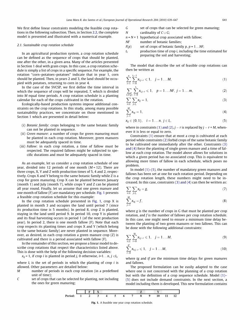
As an example, let us consider a crop rotation schedule of oneyear, divided into 12 periods of one month (M = 12). There arethree crops, X, Y and Z with production times of 5, 4 and 2, respec-tively. Crops X and Y belong to the same botanic family while Z is acrop for green manuring. Crop X can be planted between January(month 1) and July (month 7), while crops Y and Z can be plantedall year round. Finally, let us assume that one green manure andone month of fallow (F) are mandatory per schedule. Fig. 1 presentsa feasible crop rotation schedule for this example:

In the crop rotation schedule presented in Fig. 1, crop X isplanted in month 3 and occupies the land until period 7 (sinceits production time is 5 months). In period 8, crop Z is planted,staying in the land until period 9. In period 10, crop Y is plantedand its final harvesting occurs in period 1 (of the next productionyear). In period 2, there is one month fallow (F). Note that eachcrop respects its planting times and crops X and Y (which belongto the same botanic family) are never planted in sequence. More-over, as desired, in each crop rotation a green manure crop (Z) iscultivated and there is a period associated with fallow (F).

In the remainder of this section, we propose a linear model to de-scribe crop rotations that respect the characteristics listed above.This is done with the help of the following decision variables:

xij = 1, if crop i is planted in period j, 0 otherwise, i=1. . .n, j 2Ii,

where Ii is the set of periods in which the planting of crop i isallowed. Other parameters are detailed below:M number of periods in each crop rotation (in a predefined

unit of time);C set of crops that can be selected for planting, not including

the ones for green manuring;

F X Period: 1 2 3 4 5 6

Fig. 1. A feasible one year c

G set of crops that can be selected for green manuring;N cardinality of C [ G;n = N + 1 hypothetical crop associated with fallow;NF number of botanic families;F(p) set of crops of botanic family p, p = 1. . .NF;ti production time of crop i, including the time estimated for

preparing the soil and harvesting;

The model that describe the set of feasible crop rotations canthen be written as

Xn

i¼1

Xti�1

r¼0

xi;j�r 6 1; j ¼ 1 . . . M; ð1Þ

X

i2FðpÞ

Xti

r¼0

xi;j�r 6 1; p ¼ 1 . . . NF; j ¼ 1 . . . m; ð2ÞX

i2G

X

j2Ii

xij ¼ 1; ð3Þ

XM

j¼1

xnj ¼ 1; ð4Þ

xij 2 f0;1g; i ¼ 1 . . . n; j 2 Ii; ð5Þ

where in constraints (1) and (2), j � r is replaced by j � r + M, when-ever it is less or equal to zero.

Constraints (1) ensure that at most a crop is cultivated at eachperiod while constraints (2) forbid crops of the same botanic familyto be cultivated one immediately after the other. Constraints (3)and (4) force the planting of single green manure and a time of fal-low at each crop rotation. The model above allows for solutions inwhich a given period has no associated crop. This is equivalent toallowing more times of fallow in each schedule, which poses noproblem.

In model (1)–(5), the number of mandatory green manures andfallows has been set at one for each rotation period. Depending onthe crop rotation length, these numbers might need to be in-creased. In this case, constraints (3) and (4) can then be written as:X

i2G

X

j2Ii

xij ¼ g; ð7Þ

XM

j¼1

xnj ¼ f ; ð8Þ

where g is the number of crops in G that must be planted per croprotation, and f is the number of fallows per crop rotation schedule.In this case, one might need to ensure a minimum time delay be-tween the planting of two green manures or two fallows. This canbe done with the following additional constraints:

X

i2G

Xtg

r¼0

xi;j�r 6 1; j ¼ 1 . . . M; ð9Þ

Xtf

r¼0

xn;j�r 6 1; j ¼ 1 . . . M; ð10Þ

where tg and tf are the minimum time delays for green manuresand fallows.

The proposed formulation can be easily adapted to the casewhere one is not concerned with the planning of a crop rotationbut with the definition of a crop sequence schedule. Model (1)–(5) does not include demand constraints. In the next section, amodel including them is developed. This new formulation contains

Z Y 7 8 9 10 11 12

rop rotation schedule.

6 F X 2 4 2 Z Y 1 2 3 4 5 6 7 8 9 10 11 12

Fig. 2. Representation of a feasible one year crop production schedule.


an exponential number of variables and is, therefore, solved withina column-generation approach.

2.2. Crop demand supply problem

A crop rotation schedule is basically a planting calendar indicat-ing when each crop should be planted. Since the planting of a cropin a given period implies one or more subsequent harvesting peri-ods, with expected productivities, one might easily convert thecrop rotation schedule (or planting calendar) into a crop productionschedule, which is a harvesting calendar indicating the amount (inmass, volume, units or other appropriate measure) of each cropthat is being produced in each period.

Consider again the example presented in the previous sectionand illustrated in Fig. 1. Assume that crop X has its first harvestingthree months after planting and other harvesting occurs monthly,until the final harvesting, five months after the time of planting.The productions in months 3, 4 and 5 after planting are 1, 2 and1 kilogram per square meter of planted area. Crop Y has only oneharvest occurring in the last period of its production time of thefour month and its production is estimated at 3 kilograms persquare meter. With the use of this data, and assuming the plantingcalendar presented in Fig. 1 has been used in an area of 2 meter2,we can express the planting and harvesting calendar (or produc-tion scheduling) in Fig. 2. The figures in italic represent the produc-tion per meter2 of the harvesting crops.

As before, crop X is planted in month 3, crop Z in month 8, andcrop Y in month 10. The new information in the figure concerns theyields of each crop in each period. Indeed, we can now observe thatin months 5, 6 and 7, there is a production of 2, 4 and 2 kilogramsof crop X, respectively. Analogously, in month 1 there is a produc-tion of 6 kilograms of crop Y. The production of crop Z is not indi-cated since it is being used just for green manuring and has noassociated demand.

In order to model the SVCSP, one must match, at each period,the production schedule with the demands to be met of each crop.Let C be a set of crops with a known demand and A1, . . . ,AL be therespective sizes of cropping areas (which can be further dividedin the actual plots). Due, mainly, to possible heterogeneities in cli-mate and soil conditions, the set of available crops and the associ-ated productivity might differ for each cropping area. Let:

Ck, be the set of crops that can be planted in cropping area k;Sk, the set of feasible production schedules associated withcropping area k;

Now, let asijk be the amount of crop i 2 Ck produced in period j

per square meter of land in area k to which is assigned a crop rota-tion schedule s. Defining variables:

kks size of the plot associated with crop schedule s in area k.We can write the SVCSP as:

maxXL

k¼1

X

s2Sk

rkskks ð11Þ

s:t:XL

k¼1

X

s2Sk

asijkkks P dij; i 2 C; j ¼ 1 . . . M; ð12Þ

X

s2Sk

kks 6 Ak; k ¼ 1 . . . L; ð13Þ

kks P 0; s 2 Sk; k ¼ 1 . . . L; ð14Þ

where dij is the demand of crop i in period j, given in appropriateunits (kilogram, pack, etc.).

Parameter rks is the return obtained when production schedules 2 Sk is used in one square meter of cropping area k. The goal ofmodel (11)–(14) is to maximize this return which can be related,for example, to the total production volumes or revenues. Con-straints (12) ensure that the demands for all crops, at all periodsare satisfied while constraints (13) ensure that only the availableland at each area is used.

As mentioned earlier, a production schedule is completely de-fined once a crop rotation schedule has been chosen. Indeed,consider:

oi number of periods between the planting and the first harvest-ing of crop i.pikr production per m2 of the rth harvesting of crop i in the areak, for r = 1 . . . ti � oi � 1.

Given the crop rotation schedule xsk ¼ ðxs

ijkÞ, we have:

asijk ¼ pirkxs

i;j�oi�r;k; i 2 Ck; r ¼ 1 . . . ti � oi � 1; j� oi � r 2 Ii;

s 2 Sk; k ¼ 1 . . . L:

For the case where one wishes to maximize the revenueobtained by the crop rotation schedules for the L areas, theincome rks obtained for a production schedule as

k ¼ aðxsijkÞ can be

written as:

rks ¼X

i2Ck

X

j2Ii

Xti�oi�1

r¼1

cijpirkxsi;j�oi�r;k; ð15Þ

where cij is the unit price (per kilogram, per pack etc.) of crop i atperiod j.

Therefore, in terms of a crop rotation schedule xsk ¼ ðxs

ijkÞ, prob-lem (11)–(14) becomes:

maxXL

k¼1

X

s2Sk

X

i2Ck

X

j2Ii

Xti�oi�1

r¼1

cijpirkxsi;j�oi�r;kkks ð16Þ

s:t:XL

k¼1

X

s2Sk

pirxsi;j�oi�r;kkks P dij;

i 2 C; j� oi � r 2 Ii; r ¼ 1 . . . ti � oi � 1; ð17ÞX

s2Sk

kks 6 Ak; k ¼ 1 . . . L; ð18Þ

kks P 0; s 2 Sk; k ¼ 1 . . . L; ð19Þ

where j � oi � r is replaced by j � oi � r + M, whenever it is less orequal to zero.

Example. Consider 3 cropping areas with sizes A1 = 6, A2 = 4 andA3 = 5 m2. There are 8 crops, which are listed in Table 1. For eachcrop i, the table presents the botanic family (Fi) to which it belongs,the set of possible planting dates (Ii), the production times (ti), thenumber of periods before harvestings allowed (oi) and theexpected partial harvestings values, pir. For example, as o1 = 2and t1 � o1 = 2, crop 1 needs 2 periods between the planting periodand its first harvest and has 2 periods of harvests.

Table 1 also presents the demands for each one of crops 1–6, ateach period. Crops 5 and 6 are associated with green manuring andhave no associated demand.

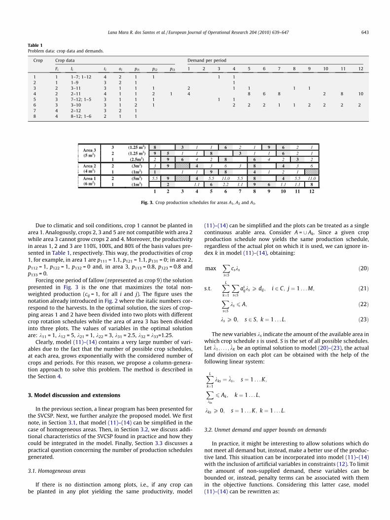
Table 1Problem data: crop data and demands.

Crop Crop data Demand per period

Fi Ii ti oi pi1 pi2 pi3 1 2 3 4 5 6 7 8 9 10 11 12

1 1 1–7; 1–12 4 2 1 1 1 12 1 1–9 3 2 1 13 2 3–11 3 1 1 1 2 1 1 1 14 2 2–11 4 1 1 2 1 4 8 6 8 2 8 105 3 7–12; 1–5 3 1 1 1 1 16 3 3–10 3 1 2 1 2 2 2 1 1 2 2 2 27 4 2–12 3 2 18 4 8–12; 1–6 2 1 1

2) 8 3 6 9 6 2) 9 5 8 3 6

2 1 2 1

Area 3 (5 m2)

2) 2 9 6 8 6

2 1 1 1

4 2 3 2 2) 3 9 4

1 1 1 1

4 2

3 6 3 8 4 Area 2 (4 m2) 2) 1 1 1 9 8 4

3 6 1 2 1

2) 5.5 9 4 8 4 Area 1 (6 m2)

3 (1.25 m2 (1.25 m1 (2.5m2 (3m1 (1m2 (5m1 (1m2) 2 1.1 6

5.5 11.0 5.5 2.2 1.1 9 6

5.5 11.0 1.1 1.1 8

1 2 3 4 5 6 7 8 9 10 11 12

Fig. 3. Crop production schedules for areas A1, A2 and A3.


Due to climatic and soil conditions, crop 1 cannot be planted inarea 1. Analogously, crops 2, 3 and 5 are not compatible with area 2while area 3 cannot grow crops 2 and 4. Moreover, the productivityin areas 1, 2 and 3 are 110%, 100%, and 80% of the basis values pre-sented in Table 1, respectively. This way, the productivities of crop1, for example, in area 1 are p111 = 1.1, p121 = 1.1, p131 = 0; in area 2,p112 = 1, p122 = 1, p132 = 0 and, in area 3, p113 = 0.8, p123 = 0.8 andp133 = 0.

Forcing one period of fallow (represented as crop 9) the solutionpresented in Fig. 3 is the one that maximizes the total non-weighted production (cij = 1, for all i and j). The figure uses thenotation already introduced in Fig. 2 where the italic numbers cor-respond to the harvests. In the optimal solution, the sizes of crop-ping areas 1 and 2 have been divided into two plots with differentcrop rotation schedules while the area of area 3 has been dividedinto three plots. The values of variables in the optimal solutionare: k11 = 1, k12 = 5, k21 = 1, k22 = 3, k31 = 2.5, k32 = k33=1.25.

Clearly, model (11)–(14) contains a very large number of vari-ables due to the fact that the number of possible crop schedules,at each area, grows exponentially with the considered number ofcrops and periods. For this reason, we propose a column-genera-tion approach to solve this problem. The method is described inthe Section 4.

3. Model discussion and extensions

In the previous section, a linear program has been presented forthe SVCSP. Next, we further analyze the proposed model. We firstnote, in Section 3.1, that model (11)–(14) can be simplified in thecase of homogeneous areas. Then, in Section 3.2, we discuss addi-tional characteristics of the SVCSP found in practice and how theycould be integrated in the model. Finally, Section 3.3 discusses apractical question concerning the number of production schedulesgenerated.

3.1. Homogeneous areas

If there is no distinction among plots, i.e., if any crop canbe planted in any plot yielding the same productivity, model

(11)–(14) can be simplified and the plots can be treated as a singlecontinuous arable area. Consider A = [ Ak. Since a given cropproduction schedule now yields the same production schedule,regardless of the actual plot on which it is used, we can ignore in-dex k in model (11)–(14), obtaining:

maxX

s2S

csks ð20Þ

s:t:XL

k¼1

X

s2S

asijks P dij; i 2 C; j ¼ 1 . . . M; ð21Þ

X

s2S

ks 6 A; ð22Þ

ks P 0; s 2 S; k ¼ 1 . . . L: ð23Þ

The new variables ks indicate the amount of the available area inwhich crop schedule s is used. S is the set of all possible schedules.Let k1; . . . ; kK be an optimal solution to model (20)–(23), the actualland division on each plot can be obtained with the help of thefollowing linear system:

XL

k¼1

kks ¼ ks; s ¼ 1 . . . K;

X

kks

6 Ak; k ¼ 1 . . . L;

kks P 0; s ¼ 1 . . . K; k ¼ 1 . . . L:

3.2. Unmet demand and upper bounds on demands

In practice, it might be interesting to allow solutions which donot meet all demand but, instead, make a better use of the produc-tive land. This situation can be incorporated into model (11)–(14)with the inclusion of artificial variables in constraints (12). To limitthe amount of non-supplied demand, these variables can bebounded or, instead, penalty terms can be associated with themin the objective functions. Considering this latter case, model(11)–(14) can be rewritten as:


maxXL

k¼1

X

s2Sk

rkskks �X

i2C

XM

j¼1

qijhij ð24Þ

s:t:XL

k¼1

X

s2Sk

asijks P dij � hij; i 2 C; j ¼ 1 . . . M; ð25Þ

X

s2Sk

kks 6 Ak; k ¼ 1 . . . L; ð26Þ

hij P 0; kks P 0; s 2 Sk; i 2 C; j ¼ 1 . . . M; k ¼ 1 . . . L; ð27Þ

where hij, is the amount of non-supplied demand of crop i in periodj, and qij is the associated penalty.

Besides allowing part of the demand to be unmet, it might beconvenient to establish an upper bound on the production. Themotivation for this would be to limit the production of the cropsto levels that can be absorbed by the farmers’ clients. This can eas-ily be done with the introduction of upper bounds on constraints(12). In Section 5, the effect of allowing unmet demands and upperbounds on production is studied.

3.3. Considerations on the number of plots

Model (11)–(14) imposes no constraints on the number of pro-duction schedules than can be used in a given area, allowing solu-tions with a very large number of plots. In order to reduce theoccurrence of these solutions, which might be impractical inreal-life situations, a penalty zk can be associated with each vari-able kks > 0. The original objective function is then replaced by:

maxXL

k¼1

X

s2Sk

ðrkskks þ zkdksÞ ð28Þ

with the following additional constraints:

kks 6 Akdks; dks ¼ f0;1g; s 2 Sk; k ¼ 1 . . . L: ð29Þ

The penalty terms zk are selected according to the desired trade-off between the number of plots in the solution and the obtainedreturn. Formulation (28), subject to constraints (12), (13) and(29) is no longer a linear programming model but a more complexmixed-integer problem. In Section 4, we discuss heuristic strate-gies for its resolution.

4. Solution approaches

Model (11)–(14) can be seen as a master program in the columngeneration framework, since it is a linear optimization problemwith a very large number of columns, which can be obtained bysolving subproblems (Lübbecke and Desrosiers, 2005). The col-umn-generation approach uses a restricted version of this masterprogram, in which only a small subset of variables (or columns)is considered. New columns are iteratively added to the restrictedmaster problem, while the procedure improves the current solu-tion. When no improving columns can be found, the current re-stricted master solution is also the solution of the master problem.

In our case, each column in the master problem is associated toa crop rotation schedule for one of the areas k. As we only considerfeasible crop rotations that respect ecologically-based criteria (i)–(iii), we can write the pricing problem as the problem of findinga crop rotation schedule that maximizes the corresponding re-duced cost, respecting constraints (1)–(5), restricted to set Ck andcrops for green manure for area k (Gk). By associating dual variablespij with constraints (12) and dual variables ak with constraints(13), the column that gives the largest reduced cost for the crop-ping area k can be obtained by solving the following pricing prob-lem Pk:

maxX

i2Ck

X

j2Ii

Xti�oi�1

r¼1

ðci;j�r � pi;j�rÞpirkxijk � ak

subject to that (xijk) satisfies (1)–(5) where only crops in Ck [ Gk areconsidered.

An algorithm for the used column-generation approach is pre-sented below:

Column-generation algorithm

1. Choose a set of initial columns to the restricted masterproblem.

2. Solve the restricted master problem and obtain (p,a), thedual variables associated with constraints (12) and (13),respectively.

3. Solve the pricing problem Pk, for k = 1. . .L, and obtain thereduced costs cks and the column as

k.4. If, for k = 1. . .L, cks=0, then stop. The current solution is

optimal. Otherwise, insert column ask with relative costs

cks > 0 in the restricted master problem and go to step 2.

At the end of the column-generation algorithm, we have a set offeasible production schedules (as

kÞ associated with given plot sizes(kksÞ. There might be a large number of kks > 0, a significant num-ber of which having tiny values. Next, we propose some strategiesto deal with this problem.

Given (ask; kksÞ, a solution for (11)–(14) containing a large num-

ber of values kks > 0, a simple way to reduce the number plots is toset each kks < d at zero, where d is a minimum desired plot size. Wename this simple strategy d-plot elimination. Another heuristic,named plot-minimization, is to select, among the columns (produc-tion schedules) present in the optimal restricted master problem,the minimum number of plots which is enough to meet the de-mand. This can be done with the aid of the following mixed-integerproblem:

minXL

k¼1

XSk

s¼1

dks ð30Þ

s:t:XL

k¼1

X

s2Sk

asijkkks P dij; i 2 C; j ¼ 1 . . . M; ð31Þ

X

s2Sk

kks 6 Ak; k ¼ 1 . . . L; ð32Þ

kks 6 Akdks; k ¼ 1 . . . L; ð33Þdks ¼ f0;1g; kks P 0; s 2 Sk; k ¼ 1 . . . L: ð34Þ

Both d-plot elimination and plot-minimization procedures lead toan increase in unused area and unmet demand. General residualstrategies for obtaining a good use of the unused area (and possiblyreducing the unmet demand) can be developed. For example, letkks, s = 1 . . .Sk, k = 1 . . .L, be an optimal solution of the master prob-lem (11)–(14) and define the residual of crop i at period j as:

rdij ¼ dij �XL

k¼1

X

s2Sk

asijkkks:

The resulting unused area can be used to increase some plotsizes in order to reduce the unmet demands. Priority can be givento crops with higher residual demands. Another option is to solve amodified version of model (11)–(14) in which the demand valuesare changed for their residual counterparts, rdij. This procedurecan be used recursively, until there is no area left to be assignedor another appropriate stopping criterion is reached.

Naturally, other procedures for dealing with the problem men-tioned in Section 3.3 exist. Among them, one can include alterna-

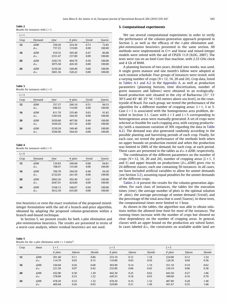
Table 2Results for instances with L = 1.

L = 1

Crop Demand time # plots %resid %oarea

12 d200 250.20 224.30 0.73 72.85d1 757.25 119.80 0.00 100.00

16 d200 910.35 395.40 0.47 86.88d1 2331.47 237.00 0.00 100.00

20 d200 3283.76 494.70 0.50 100.00d1 3075.58 426.30 0.00 100.00

24 d200 3230.28 549.40 0.60 100.00d1 3601.36 528.22 0.00 100.00


L = 3


12 d200 257.37 266.10 0.51 84.53d1 646.62 116.89 0.00 100.00

16 d200 811.76 335.40 0.63 91.82d1 1283.94 244.50 0.00 100.00

20 d200 2630.80 497.90 0.49 100.00d1 3430.26 457.56 0.00 100.00

24 d200 3230.28 549.40 0.60 100.00d1 3596.96 594.50 0.00 100.00


L = 5


12 d200 129.83 249.60 0.68 64.81d1 708.97 135.60 0.00 100.00

16 d200 766.70 394.50 0.48 94.30d1 2722.03 241.50 0.00 100.00

20 d200 2062.26 502.40 0.67 100.00d1 2947.01 424.80 0.00 100.00

24 d200 3168.13 546.67 0.60 100.00d1 3612.39 635.89 0.00 100.00


tive heuristics or even the exact resolution of the proposed mixed-integer formulation with the aid of a branch-and-price algorithm,obtained by adapting the proposed column-generation within abranch-and-bound technique.

In Section 5, we present results for both d-plot elimination andplot-minimization heuristics. The results are presented in terms ofa worst-case analysis, where residual heuristics are not used.

Table 5Results for the a-plot elimination with d = 1 meter2.

Crop dmax L = 1 L = 3

# plots %darea %lostde # plots

12 d200 201.40 0.11 0.86 233.10d1 114.70 0.03 0.15 110.00

16 d200 336.60 0.26 0.68 303.90d1 221.50 0.07 0.42 232.00

20 d200 432.00 0.30 1.30 442.30d1 378.80 0.23 1.22 420.33

24 d200 478.20 0.33 1.32 478.20d1 469.44 0.26 0.93 529.80

5. Computational experiments

We ran several computational experiments in order to verifythe performance of the column-generation approach proposed inSection 3, as well as the efficacy of the d-plot elimination andplot-minimization heuristics presented in the same section. Allmethods were implemented in C++ and linear and mixed-integermodels were solved with the aid of CPLEX 11.0 (ILOG, 2007). Thetests were run on an Intel Core Duo machine, with 2.33 GHz clockand 4 Gb of RAM.

A planning horizon of two years, divided into weeks, was used.A single green manure and one month’s fallow were adopted ateach rotation schedule. Four groups of instances were tested, witha varying number of crops (N = 12, 16, 20 and 24). Crop data, listedin Tables A.1 and A.2 in the Appendix A, as well as productionparameters (planning horizon, time discretization, number ofgreen manures and fallows) were obtained in an ecologically-based production unit situated in the city of Barbacena (21� 130

3000S and 43� 460 2500 W, 1165 meters above sea level), in the coun-tryside of Brazil. For each group, we tested the performance of thealgorithm for a different number of cropping areas: L = 1, 3 or 5.Case L = 1 is associated with the homogeneous area problem, de-tailed in Section 3.1. Cases with L = 3 and L = 5 corresponding toheterogeneous areas were manually generated. A set of crops wereselected as feasible for each cropping area, with varying productiv-ity (with a maximum variation of 30% regarding the data in TableA.2). The demand was also generated randomly according to thepossible planting and harvesting periods of each crop. Finally, foreach case, we tested the performance of the methods both whenno upper bounds on production existed and when the productionwas limited to 200% of the demand, for each crop, at each period.These cases are presented in the tables as d1 e d200, respectively.

The combination of the different parameters on the number ofcrops (N = 12, 16, 20 and 24), number of cropping areas (L = 1, 3and 5) and upper bounds on productions (d1,d200) gives rise to24 different classes, each one containing 50 instances. In all cases,we have included artificial variables to allow for unmet demands(see Section 3.2), assuming equal penalties for the unmet demandsof the different crops.

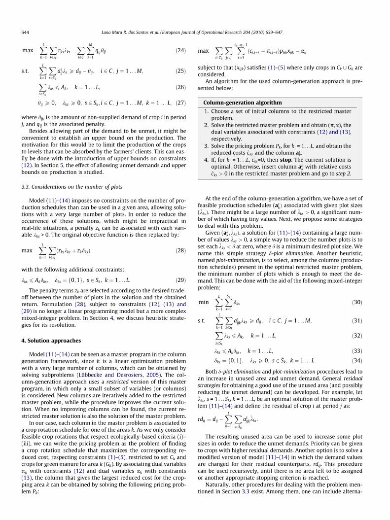
Tables 2–4 present the results for the column-generation algo-rithm. For each class of instances, the tables list the executiontimes (time), the average number of plots in the optimal solution(# plots), the average percentage of unmet demand (%resid), andthe percentage of the total area that is used (%oarea). In these tests,the computational times were limited to 1 hour.

As shown in the tables, the algorithm was able to obtain solu-tions within the allowed time limit for most of the instances. Therunning times increase with the number of crops but showed noclear dependency on the number of cropping areas. In general,classes with an upper bound on the production are solved faster.In cases labeled d1, the constraints on available arable land are

L = 5

%darea %lostde # plots %darea %lostde

0.15 1.18 224.80 0.12 1.540.03 0.50 128.30 0.04 0.38

0.14 1.19 351.10 0.19 0.620.06 0.42 230.10 0.06 0.38

0.25 0.62 443.50 0.27 1.060.18 0.93 390.60 0.16 0.70

0.33 1.32 487.89 0.28 1.400.31 1.49 561.67 0.35 1.68

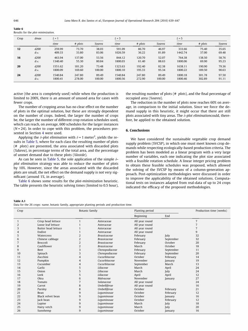
Table 6Results for the plot-minimization.

Crop dmax L = 1 L = 3 L = 5

time # plots %oarea time # plots %oarea time # plots %oarea

12 d200 259.99 73.70 38.03 591.09 86.70 46.97 333.66 75.40 35.65d1 409.33 33.80 83.06 1026.59 36.22 81.89 1442.74 37.00 69.48

16 d200 463.94 137.00 53.56 844.12 120.70 52.07 764.38 138.50 58.76d1 1340.40 55.30 80.84 1800.03 61.40 88.63 1800.06 69.90 95.23

20 d200 1551.62 181.20 73.48 1323.63 192.40 82.38 1638.11 190.90 79.36d1 1800.09 169.60 100.00 1800.10 195.33 95.34 1800.22 189.50 90.63

24 d200 1540.84 247.80 89.49 1540.84 247.80 89.49 1800.18 301.78 97.50d1 1800.41 278.00 100.00 1800.56 272.90 100.00 1800.46 302.89 91.11


active (the area is completely used) while when the production islimited to 200%, there is an amount of unused area for cases withfewer crops.

The number of cropping areas has no clear effect on the numberof plots in the optimal solution, but these are strongly dependenton the number of crops. Indeed, the larger the number of cropsbe, the larger the number of different crop rotation schedules used,which can reach, on average, 600 schedules for the larger instances(N = 24). In order to cope with this problem, the procedures pre-sented in Section 4 were used.

Applying the d-plot elimination with d = 1 meter2, yields the re-sults in Table 5, where for each class the resulting number of plots(# plots) are presented, the area associated with discarded plots(%darea), in percentage terms of the total area, and the percentageof unmet demand due to these plots (%lostde).

As can be seen in Table 5, the sole application of the simple d-plot elimination strategy was able to reduce the number of plotsby 10%. However, since the areas associated with the discardedplots are small, the net effect on the demand supply is not very sig-nificant (around 1%, in average).

Table 6 shows some results for the plot-minimization heuristic.The table presents the heuristic solving times (limited to 0.5 hour),

Table A.1Data for the 26 crops: name, botanic family, appropriate planting periods and production

Crop Botanic family

1 Crisp head lettuce 1 Asteraceae2 Loose leaf lettuce 1 Asteraceae3 Butter head lettuce 1 Asteraceae4 Endive 1 Asteraceae5 Watercress 2 Brassicaceae6 Chinese cabbage 2 Brassicaceae7 Broccoli 2 Brassicaceae8 Cauliflower 2 Brassicaceae9 Beet 3 Chenopodiaceae10 Spinach 3 Chenopodiaceae11 Zucchini 4 Cucurbitaceae12 Pumpkin 4 Cucurbitaceae13 Cucumber 4 Cucurbitaceae14 Garlic 5 Liliaceae15 Onion 5 Liliaceae16 Leek 5 Liliaceae17 Okra 6 Malvaceae18 Tomato 7 Solanaceae19 Carrot 8 Umbelliferae20 Parsley 8 Umbelliferae21 Bean 9 Leguminosae22 Black velvet bean 9 Leguminosae23 Jack bean 9 Leguminosae24 Lupine 9 Leguminosae25 Hairy vetch 9 Leguminosae26 Sunnhemp 9 Leguminosae

the resulting number of plots (# plots), and the final percentage ofoccupied area (%oarea).

The reduction in the number of plots now reaches 60% on aver-age, in comparison to the initial solution. Since we force the de-mand supply in this heuristic, it might occur that there are stillplots associated with tiny areas. The d-plot eliminationcould, there-fore, be applied to the obtained solution.

6. Conclusions

We have considered the sustainable vegetable crop demandsupply problem (SVCSP), in which one must meet known crop de-mands while respecting ecologically-based production criteria. Theproblem has been modeled as a linear program with a very largenumber of variables, each one indicating the plot size associatedwith a feasible rotation schedule. A linear integer pricing problemto obtain these feasible schedules was proposed, which allowedthe solving of the SVCSP by means of a column-generation ap-proach. Post-optimization methodologies were discussed in orderto improve the applicability of the obtained solutions. Computa-tional tests on instances adapted from real-data of up to 24 cropsindicated the efficacy of the proposed methodologies.

time.

Planting period Production time (weeks)

Beginning End

All year round 7All year round 7All year round 7All year round 9February July 32February September 32February October 20March October 18February September 11February September 20October February 14November January 19September March 13March April 24March July 24April April 12November January 27All year round 24All year round 16October February 21October February 12October January 16October February 12March July 18March July 20October January 16

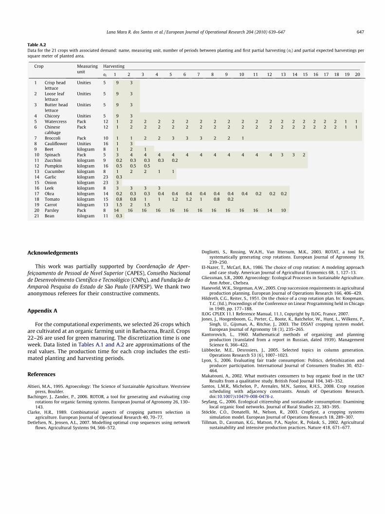
Table A.2Data for the 21 crops with associated demand: name, measuring unit, number of periods between planting and first partial harvesting (oi) and partial expected harvestings persquare meter of planted area.


Acknowledgements

This work was partially supported by Coordenação de Aper-feiçoamento de Pessoal de Nıvel Superior (CAPES), Conselho Nacionalde Desenvolvimento Cientıfico e Tecnológico (CNPq), and Fundação deAmparoà Pesquisa do Estado de São Paulo (FAPESP). We thank twoanonymous referees for their constructive comments.

Appendix A

For the computational experiments, we selected 26 crops whichare cultivated at an organic farming unit in Barbacena, Brazil. Crops22–26 are used for green manuring. The discretization time is oneweek. Data listed in Tables A.1 and A.2 are approximations of thereal values. The production time for each crop includes the esti-mated planting and harvesting periods.

References

Altieri, M.A., 1995. Agroecology: The Science of Sustainable Agriculture. Westviewpress, Boulder.

Bachinger, J., Zander, P., 2006. ROTOR, a tool for generating and evaluating croprotations for organic farming systems. European Journal of Agronomy 26, 130–143.

Clarke, H.R., 1989. Combinatorial aspects of cropping pattern selection inagriculture. European Journal of Operational Research 40, 70–77.

Detlefsen, N., Jensen, A.L., 2007. Modelling optimal crop sequences using networkflows. Agricultural Systems 94, 566–572.

Dogliotti, S., Rossing, W.A.H., Van Ittersum, M.K., 2003. ROTAT, a tool forsystematically generating crop rotations. European Journal of Agronomy 19,239–250.

El-Nazer, T., McCarl, B.A., 1986. The choice of crop rotation: A modeling approachand case study. American Journal of Agricultural Economics 68, 1, 127–13.

Gliessman, S.R., 2000. Agroecology: Ecological Processes in Sustainable Agriculture.Ann Arbor., Chelsea.

Haneveld, W.K., Stegeman, A.W., 2005. Crop succession requirements in agriculturalproduction planning. European Journal of Operations Research 166, 406–429.

Hildreth, C.G., Reiter, S., 1951. On the choice of a crop rotation plan. In: Koopmans,T.C. (Ed.), Proceedings of the Conference on Linear Programming held in Chicagoin 1949, pp. 177–188.

ILOG CPLEX 11.1 Reference Manual, 11.1, Copyright by ILOG, France, 2007.Jones, J., Hoogenboom, G., Porter, C., Boote, K., Batchelor, W., Hunt, L., Wilkens, P.,

Singh, U., Gijsman, A., Ritchie, J., 2003. The DSSAT cropping system model.European Journal of Agronomy 18 (3), 235–265.

Kantorovich, L., 1960. Mathematical methods of organizing and planningproduction (translated from a report in Russian, dated 1939). ManagementScience 6, 366–422.

Lübbecke, M.E., Desrosiers, J., 2005. Selected topics in column generation.Operations Research 53 (6), 1007–1023.

Lyon, S., 2006. Evaluating fair trade consumption: Politics, defetishization andproducer participation. International Journal of Consumers Studies 30, 452–464.

Makatouni, A., 2002. What motivates consumers to buy organic food in the UK?Results from a qualitative study. British Food Journal 104, 345–352.

Santos, L.M.R., Michelon, P., Arenales, M.N., Santos, R.H.S., 2008. Crop rotationscheduling with adjacency constraints. Annals of Operations Research.doi:10.1007/s10479-008-0478-z.

Seyfang, G., 2006. Ecological citizenship and sustainable consumption: Examininglocal organic food networks. Journal of Rural Studies 22, 383–395.

Stöckle, C.O., Donatelli, M., Nelson, R., 2003. CropSyst, a cropping systemssimulation model. European Journal of Operations Research 18, 289–307.

Tillman, D., Cassman, K.G., Matson, P.A., Naylor, R., Polask, S., 2002. Agriculturalsustainability and intensive production practices. Nature 418, 671–677.

http://dx.doi.org/10.1007/s10479-008-0478-z

Documents

Sustainable vegetable crop supply problem