Swiss National Bank Economic Studies · 2017-05-05 · Swiss National Bank Economic Studies No. 6 2009 A VECX* model of the Swiss economy* Katrin Assenmacher-Weschea and M. Hashem

Swis

s Na

tion

al B

ank

Econ

omic

Stu

dies

No.

6

2009

A VECX* model of the Swiss economy Katrin Assenmacher-Wesche and M. Hashem Pesaran

Copies of Swiss National Bank Economic Studies may be obtained from:

Swiss National Bank, Library, Fraumünsterstrasse 8, P.O. Box, CH-8022 Zurich

Fax: +41 44 631 81 14

E-mail: [email protected]

This publication is also available on the SNB website (www.snb.ch).

Economic Studies represent the views of the authors and do not necessarily refl ect those of the

Swiss National Bank.

Copyright ©

The Swiss National Bank (SNB) respects all third-party rights, in particular rights relating to works

protected by copyright (information or data, wordings and depictions, to the

extent that these are of an individual character).

SNB publications containing a reference to a copyright (© Swiss National Bank/SNB, Zurich/year,

or similar) may, under copyright law, only be used (reproduced, used via the internet, etc.) for

non-commercial purposes and provided that the source is mentioned.

Their use for commercial purposes is only permitted with the prior express consent of the SNB.

General information and data published without reference to a copyright may be used without

mentioning the source.

To the extent that the information and data clearly derive from outside sources, the users of such

information and data are obliged to respect any existing copyrights and to obtain the right of use

from the relevant outside source themselves.

Limitation of liability

The SNB accepts no responsibility for any information it provides. Under no circumstances will it

accept any liability for losses or damage which may result from the use of such information.

This limitation of liability applies, in particular, to the topicality, accuracy, validity and availability

of the information.

ISSN 1661-142X (printed version)

ISSN 1661-1438 (online version)

© 2009 by Swiss National Bank, Börsenstrasse 15, P.O. Box, CH-8022 Zurich

Swiss National Bank Economic StudiesNo. 6 2009

A VECX* model of the Swiss economy*

Katrin Assenmacher-Weschea and M. Hashem Pesaranb

* The views expressed in this paper are solely our own and not necessarily shared by the Swiss National Bank. We are grateful to an anonymous referee and the editors of the SNB Economic Studies for helpful comments.

a Swiss National Bank, P.O. Box, CH-8022 Zurich, [email protected] University of Cambridge, [email protected]

2

Contents

Abstract (Zusammenfassung, Résumé) 21. Introduction 42. Modeling choices 5

2.1 Data on the core variables 62.2 Single equation ARDL models: a preliminary data analysis 72.3 Unit root test results 12

3. System approach: econometric methodology 144. Empirical results 17

4.1 Lag lengths and deterministic components 174.2 The long-run structural model 174.3 Error-correction equations 224.4 Generalized impulse responses and persistence profi les 22

5. Conclusions 29Appendix: Sources and construction of data 45

Swiss data 45Foreign data 45

References 50

Abstract

This paper applies the modelling strategy of Garratt, Lee, Pesaran and Shin (2003) to the estimation of a structural cointegrated VAR model that relates the core macr-oeconomic variables of the Swiss economy to current and lagged values of a number of key foreign variables. We identify and test a long-run structure between the vari-ables. Moreover, we analyse the dynamic properties of the model using Generalised Impulse Response Functions. In its current form the model can be used to produce forecasts for the endogenous variables either under alternative specifi cations of the marginal model for the exogenous variables, or conditional on some pre-specifi ed path of those variables (for scenario forecasting). In due course the Swiss VECX* model can also be integrated within a Global VAR (GVAR) model where the foreign variables of the model are determined endogenously.

JEL classifi cation: C53, C32Keywords: Long-run structural vector autoregression

Zusammenfassung

In diesem Aufsatz wird der Modellansatz von Garratt, Lee, Pesaran und Smith (2003) zur Schätzung eines strukturellen kointegrierten Fehlerkorrekturmodells verwendet, das wesentliche makroökonomische Variable für die Schweiz unter Berücksichtigung gegenwärtiger und verzögerter Werte relevanter Zeitreihen für das Ausland erklärt. Es werden theoretisch motivierte, langfristige Beziehungen zwischen den Variablen

3

identifi ziert und getestet. Ausserdem werden die dynamischen Eigenschaften des Modells anhand generalisierter Impuls-Antwort-Folgen analysiert. In seiner gegen-wärtigen Form kann das Modell zur Prognose der endogenen Variablen verwendet werden, wobei diese Prognosen entweder auf eine bestimmte Spezifi kation eines marginalen Modells für die exogenen Variablen oder auf einen vorgegebenen Pfad für diese Variablen (Szenario-Prognosen) bedingt werden können. Zu gegebener Zeit kann dieses VECX* Modell für die Schweiz in ein globales vektorautoregressives (GVAR) Modell eingefügt werden, in welchem die exogenen Variablen ebenfalls endogen erklärt werden.

Résumé

Les auteurs du présent article se servent de la stratégie de modélisation de Garratt, Lee, Pesaran et Shin (2003) pour évaluer un modèle VAR structurel cointégré, qui met les principales variables macroéconomiques de la Suisse en relation avec plusieurs variables-clés actuelles et retardées de l’étranger. Ils distinguent et testent des structures à long terme reliant les différentes variables. De plus, les auteurs analysent les propriétés dynamiques du modèle à l’aide de fonctions généralisées de réponse aux impulsions (Generalised Impulse Response Functions). Sous sa forme actuelle, le modèle peut être utilisé afi n d’établir des prévisions portant sur les variables endogènes à l’aide de spécifi cations alternatives du modèle marginal pour les variables exogènes ou de valeurs prédéfi nies pour ces variables (prévision de scénarios). En temps utile, le modèle suisse VECX* peut également être intégré au modèle Global VAR (GVAR), dans lequel les variables étrangères sont déterminées de manière endogène.

4

1. Introduction

At the end of 1999 the Swiss National Bank (SNB) abandoned monetary targeting in favour of maintaining price stability by announcing an explicit infl ation objective in terms of an annual increase in the consumer price index (CPI) of at most two percent. Under the new monetary policy regime the infl ation forecast plays a central role. The SNB employs different types of models to form a consensus forecast for the infl ation rate. These include a large simultaneous equation model, a small structural model, structural and non-structural vector autoregressive (VAR) models, and a small structural cointegrating VAR model.

The structural cointegrating VAR approach is particularly attractive as it com-bines long-run information from economic theory with a fl exible modelling of the short-run dynamics. The structural cointegrating VAR model previously used at the SNB, however, had some shortcomings as it considered only domestic vari-ables. Infl ation in Switzerland, being a small open economy, is strongly infl uenced by developments in the rest of the world. A forecasting model that takes account of foreign infl uences on domestic variables is therefore desirable.

This paper develops a long-run structural cointegrating VAR model that relates the core macroeconomic variables of the Swiss economy to current and lagged values of a number of key foreign variables, following the approach of Garratt, Lee, Pesaran and Shin (2003, 2006). We refer to this model as the Swiss VECX* model. In a structural cointegrating VAR model the implications of economic theory for the long-run relations among the variables in the model are combined with a data-driven approach to modeling the short-run dynamics. The Swiss VECX* model is estimated on quarterly data over the period 1976Q1 to 2006Q4. The endogenous variables are real M2, real gross domestic product (GDP), the three-month LIBOR rate, the quarterly rate of infl ation, the nominal exchange rate, and the ratio of the domestic to the foreign price level. The weakly exogenous variables are foreign real GDP, the foreign three-month interest rate, and the oil price. In the Swiss VECX* model fi ve long-run relations are identifi ed. These are purchasing power parity, money demand, the uncovered interest parity linking the domestic to the foreign interest rate, a rela-tion between domestic and foreign output, and a modifi ed Fisher equation that relates the domestic interest rate to the domestic infl ation rate. Though the overidentifying restrictions implied by economic theory were marginally rejected, the diagnostic tests confi rm that the model seems to provide a good explanation of the Swiss data.

We also provide a detailed analysis of the dynamic properties of the VECX* model by means of impulse response functions. The impulse response function, which considers the effects of a typical shock on the time path of the variables in the model, is the standard tool for the analysis of interactions and dynamics. One can consider shocks to observable or unobservable variables. The effect of a shock to an observable on the other variables is of considerable interest in itself and should certainly be the fi rst stage of any analysis. Shocks to observables are calculated using Generalized Impulse Response Functions, GIRFs. The calculation of GIRF‘s does not require any identifying assumptions and uses the estimated error covari-ances to allow for the contemporaneous linkages that have prevailed between shocks historically.

5

However, for some purposes, we may wish to know the economic nature of the shocks to observables. For interest rates we may wish to decompose the observable shock to the interest rate into a domestic monetary policy shock, a foreign monetary policy shock and a residual shock. To be able to produce conditional forecasts given a specifi c path for the short-term interest rate, a monetary policy shock has to be identi-fi ed. Decomposing the observable shock into its unobserved components requires more information, which is often supplied by the economic theory of the short run. This topic, however, is not part of the current study.

The forecast performance of the VECX* model is investigated by Assenmacher-Wesche and Pesaran (2008), who show that the model is capable of generating reasonable out-of-sample forecasts for output, infl ation and the interest rate over the period 2000Q1 to 2006Q4, when compared to a number of benchmark forecasts. In their forecasting exercise forecasts for the exogenous variables come from a marginal model for the exogenous variables. Nevertheless, the model can also be used for scenario forecasts, in which the evolution of the exogenous variables is based on the scenarios developed in the “Weltwirtschaftliche Annahmen”, as it is the case for the other SNB models that include foreign variables. A more consistent approach, however, would be to obtain the forecasts for the exogenous variables from a Global VAR recently proposed in Pesaran, Schuermann, and Weiner (2004) and further developed in Dees, di Mauro, Pesaran and Smith (2007). The Swiss VECX* model is designed such that it can be readily linked to a Global VAR model, but this is not part of the current paper.

The outline of the rest of the paper is as follows. Section 2 introduces the data, examines the time-series properties of the variables to be included in the model, and presents a preliminary univariate analysis of the long-run relations. Section 3 sets out the econometric methodology used. Section 4 presents the empirical results. Section 5 ends with some concluding remarks.

2. Modeling choices

The model considered in this study is a structural cointegrated VAR model that relates the core macroeconomic variables of the Swiss economy (denoted by the vector xt ) to current and lagged values of a number of key foreign variables (denoted by the vector x∗

t ), which we call the Swiss VECX* model. The foreign variables are constructed specifi cally to refl ect the interlinkages of the Swiss economy with the rest of the world, particularly the euro area. As shown in Pesaran and Smith (2006) the VECX* model can be derived as the solution to an open macro economy New Keynesian Dynamic Stochastic General Equilibrium (DSGE) model. Therefore, it is possible in principle to impose the short-run and long-run DSGE-type parametric restrictions on the VECX* model, although at this stage we shall focus on the long-run relations and leave the short-run parameters unrestricted.

In the implementation of the long-run structural modelling a number of choices have to be made, see Garratt et al. (2006, p. 114). Among these are the choice of the core endogenous and exogenous variables, their lag orders, the deterministics (namely the choice of intercept and linear trends) and the sample period. The choice of the variables is infl uenced by the purpose of the model, namely forecasting the

6

rate of infl ation and modeling the monetary policy process. Therefore, the model should incorporate those key relations from economic theory that can be expected to have an impact on the infl ation rate. One of these relations is money demand, which postulates a long-run relation between the real money stock, real output and the interest rate. Another is an interest rate rule which establishes a long-run relation between the interest rate and infl ation. Switzerland as a small, open economy can be expected to be subject to infl uences from the exchange rate. Therefore, purchasing power parity, which links the domestic price level to the nominal exchange rate and the foreign price level, is also included. In addition, we consider the price of oil as the most important commodity price, which is expected to have direct and indirect impacts on world infl ation. Finally, international business cycles and interest rate cycles are allowed to have an infl uence on the domestic economy by considering long-run relations between domestic and foreign output and interest rates. The latter two variables, together with the oil price, are regarded as exogenous variables.

2.1 Data on the core variables

The data are quarterly and run from the fi rst quarter of 1974 to the last quarter of 2006. The domestic variables are (log) real M2, mt, (log) real gross domestic product (GDP), yt, the three-month LIBOR rate, rt, and the quarterly rate of infl ation, πt. These variables are treated as endogenous. Further endogenous variables are the nominal exchange rate, et, and the ratio of the (log) domestic to the (log) foreign price level, pt – pt

∗. The exogenous variables are (log) foreign real GDP, yt∗, the foreign

three-month interest rate, rt∗, and the (log) oil price, pt

oil. Except for the interest rates, all the series are in logarithms. Interest rates are expressed as 0.25ln(1 + R / 100) where R is the interest rate in percent per annum to make units of measurement compatible with the rate of infl ation, which is computed as the fi rst difference of the logarithm of the quarterly price level.

The foreign (star) variables are computed as weighted averages, using three-year moving averages of the trade shares with Switzerland. For example, the foreign output is computed as

=1

= ,N

t jt jtj

y w y∗ ∑

where yjt is the logarithm of real output of country j, and wjt is its associated weight. Foreign output and the foreign price level are aggregates of the GDP and the con-sumer price indices (CPI) of Switzerland‘s 15 largest trade partners. The quarterly trade weights are computed as averages of the Swiss economy‘s imports from and exports to the country in question divided by the total trade of all the 15 countries. Trade to these 15 countries on average covers about 82 percent of total Swiss foreign trade. Chart A.3 in the appendix shows the evolution of the trade weights. Germany is the most important trading partner of Switzerland — accounting for a trade share of about 30 percent — followed by France, Italy and the United States. Out of the 15 major trading partners, eleven are European economies that account for as much as 83 percent of the Swiss trade. The trade with the US amounts to around 9 percent of Swiss trade, with Asian countries picking up the rest. The exchange rate and

7

the foreign interest rate variables are computed as averages of the US and the euro area time series only, given the dominance of these two regions in Swiss fi nancial markets. A detailed description of the variables, their sources, and the construction of the foreign variables is given in the appendix.

Economic theory predicts a number of long-run relations such as purchasing power parity (pt – pt

∗ – et, PPP), the Fisher parity (rt – πt ), and the uncovered interest parity (rt – rt

∗, UIP); see Garratt, Lee, Pesaran and Shin (2006) for further details. We shall also consider a modifi ed version of the Fisher Parity where we relax the unit coeffi cient restriction on the infl ation rate. We refer to this version as the long-run interest rate rule (rt – βπt, LIR).

The extent to which these long-run relations have held historically are depicted graphically in Charts 1 to 7 where levels and fi rst differences of the various vari-ables that are expected to enter the long-run relations are displayed. Chart 1 shows the variables in the PPP relationship, namely the weighted average of the nominal exchange rate of the Swiss franc against the euro area and the US, together with the ratio of the domestic to the foreign price level. Apparently both variables share the same trend in the long run, suggesting that PPP could be one of the long-run relations. Nevertheless, there seems to be some trend real appreciation over the sample period since the relative price level falls by more than the exchange rate, which we will take into account later. Chart 2 shows the evolution of real M2 and real GDP. The fact that both series have similar trend properties suggests an income elasticity of close to unity. Chart 3 plots the velocity of M2 against the short-term interest rate. Movements in velocity coincide well with swings in the interest rate, especially since the 1980s. Chart 4 shows that the domestic and foreign real output series also seem to share similar trend properties. From the mid-1980s on, however, Swiss output growth has not been keeping up with the foreign output growth, and this needs to be taken into account. Chart 5 shows the domestic and foreign three-month interest rates. Both move closely together, though the gap between foreign and domestic interest rates that has been present in the late 1970s and early 1980s narrows slightly during the 1990s. One possible explanation is that the foreign countries have reduced their infl ation rate more strongly than Switzerland, which traditionally has experienced a relatively low rate of infl ation. Chart 6 shows the relation between the domestic three-month interest rate and the rate of infl ation. In the 1970s there have been times of negative (ex post) real interest rates while throughout the 1990s the real interest rate has been positive. Finally, Chart 7 shows the evolution of oil prices.

2.2 Single equation ARDL models: a preliminary data analysis

Before embarking on a system estimation of all the long-run relations it is instructive to consider single-equation estimation of each of the long-run relations using the autoregressive distributed lag (ARDL) modeling approach detailed in Pesaran and Shin (1999) and Pesaran, Shin and Smith (2001). Since the Swiss VECX* model will contain nine variables and thus is rather large it is advisable to fi rst investigate possible cointegrating relations in smaller sub-systems. The ARDL approach allows for such a preliminary analysis of the long-run relationships between groups of vari-ables separately before combining them in a full system estimation. Ho and Sørensen (1996) show that under or over-estimation of the cointegrating rank becomes more

8

Chart 1: EXCHANGE RATE AND RATIO OF DOMESTIC TO FOREIGN PRICES

75 80 85 90 95 00 05

×10–1

3.0

2.0

1.0

0.0

–1.0

–2.0

–3.0

×10–1

5.6

4.2

2.8

1.4

0.0

–1.4

–2.8 75 80 85 90 95 00 05

×10–2

–6.0

4.0

2.0

0.0

–0.2

–0.4

–0.6

–0.8

–1.0

–1.2

×10–2

–1.2

0.8

0.4

0.0

–0.4

–0.8

–1.2

–1.6

–2.0

–2.4

Level First difference

Chart 2: REAL M2 AND GDP

75 80 85 90 95 00 05

×101.34

1.32

1.30

1.28

1.26

1.24

1.22

×101.17

1.16

1.15

1.14

1.13

1.12

11.1 75 80 85 90 95 00 05

×10–2

–7.5

5.0

2.5

0.0

–2.5

–5.0

–7.5

×10–2

3.0

1.5

0.0

–1.5

–3.0

–4.5

–6.0


Chart 3: M2 VELOCITY AND THREE-MONTH INTEREST RATE

75 80 85 90 95 00 05

–1.04

–1.12

–1.20

–1.28

–1.36

–1.44

–1.52

–1.60

×10–2

3.0

2.5

2.0

1.5

1.0

0.5

0.0

–0.5 75 80 85 90 95 00 05

×10–1

–1.00

0.75

0.50

0.25

0.00

–0.25

–0.50

–0.75

×10–2

–0.75

0.5

0.25

0.0

–0.25

–0.50

–0.75

–1.00


9

Chart 4: DOMESTIC AND FOREIGN GDP

75 80 85 90 95 00 05

11.8

11.7

11.6

11.5

11.4

11.3

11.2

11.1

×10–1

3.0

1.5

0.0

–1.5

–3.0

–4.5

–6.0

–7.5 75 80 85 90 95 00 05

×10–2

3.0

2.0

1.0

0.0

–1.0

–2.0

–3.0

–4.0

–5.0

–6.0

×10–2

3.0

2.0

1.0

0.0

–1.0

–2.0

–3.0

–4.0

–5.0

–6.0


Chart 5: DOMESTIC AND FOREIGN THREE-MONTH INTEREST RATE

75 80 85 90 95 00 05

×10–2

3.0

2.5

2.0

1.5

1.0

0.5

0.0 75 80 85 90 95 00 05

×10–2

0.75

0.50

0.25

0.00

–0.25

–0.50

–0.75

–1.00


Chart 6: THREE-MONTH INTEREST RATE AND INFLATION

75 80 85 90 95 00 05

×10–2

3.0

2.5

2.0

1.5

1.0

0.5

0.0

–0.5 75 80 85 90 95 00 05

×10–2

1.5

1.0

0.5

0.0

–0.5

–1.0

–1.5


10

serious the larger the number of endogenous variables being considered. The ARDL models thus will give evidence on which of the long-run relations from theory may hold in the data and help in determination of the number of cointegrating relations when we come to full system estimation. In addition, we obtain coeffi cient estimates of the long-run parameters from the ARDL models. Since it is often diffi cult to iden-tify the cointegrating space of a high-dimensional system by choosing restrictions that are economically meaningful and not rejected by the data, the estimates from the ARDL long-run relations will indicate which parameter restrictions are likely to be accepted and thus can provide a cross check for the estimated β vector. To preview the results, we fi nd that no unexplainable differences between the sub-system ARDL and the full system estimates arise.

Finally, the ARDL approach is robust to the unit-root properties of the underlying series and knowledge of the order of integration of the variables is not necessary. This allows one to test for the existence of a long-run relation without having to pretest variables for a unit root, which will be particularly helpful in the case of infl ation that may be either I (1) or I (0), depending on the sample period.

To investigate the existence of a long-run relation, an ARDL regression in error-correction form is estimated and it is tested whether lagged levels of the variables enter the regression in a statistically signifi cant manner. Alternatively, the signifi -cance of the coeffi cient on the error-correction term can be tested. The test statistics follow a non-standard distribution, irrespective of whether the variables included in the model are I (1) or I (0). Pesaran, Shin and Smith (2001) provide critical values for a F-test of the exclusion of the lagged levels and for a t-test of the signifi cance of the error-correction term. Depending on whether the variables are I (1) or I (0), the critical values tabulated in Pesaran, Shin and Smith (2001) provide a lower and an upper bound for the null hypothesis of no cointegration. When the test statistic lies below the lower bound, the null hypothesis cannot be rejected. When it lies above the upper bound, the null is rejected, whereas when it lies between the lower and the upper bound, the result depends on whether the variables are I (0) or I (1). The critical

Chart 7: OIL PRICE

75 80 85 90 95 00 05

4.25

4.00

3.75

3.5

3.25

3.0

2.75

–2.5

2.25 75 80 85 90 95 00 05

×10–1

6.0

4.0

2.0

0.0

–2.0

–4.0

–6.0


11

values also depend on the characteristics of the deterministic variables, i.e., whether a trend or a constant are included in the model and — in case of the F-test — whether the intercepts or the trend coeffi cients are restricted or not.

The sub-models we investigate correspond to the fi ve long-run relations we expect to fi nd among the variables in the model: purchasing power parity, money demand, the relation between domestic and foreign output, the relation between domestic and foreign interest rates and the relation between the interest rate and infl ation. The number of lags in each of the sub-models is selected by the Akaike Information Criterion (AIC), considering a maximum lag length of four. The estimation period runs from 1976Q1 to 2006Q4. We include linear trends in the case of the regressions for PPP and the output gap since inspection of Chart 1 and Chart 4 indicated that a trend may be present. The results of the ARDL regressions are shown in Table 1. The columns two to four of Table 1 show the error-correction term, its t-ratio and the lower and upper bound critical values. The next two columns give the F-statistic for exclusion of the levels of the variables and the respective upper and lower criti-cal values. The last two columns show the adjusted R2 and the specifi cation of the ARDL model. All estimated models show a signifi cantly negative error-correction coeffi cient. The t-statistic exceeds the upper bound in absolute value for all ARDL models except for the uncovered interest parity, where it falls between the upper and the lower bound. The F-statistic always exceeds the upper bound and thus rejects the hypothesis of no level effects in the ARDL specifi cations. The evidence thus indicates the existence of fi ve stable long-run relations in the ARDL models. The estimated long-run relations from the ARDL models are given below:

Purchasing power parity (PPP): 1

(0.090) (0.0007)(0.22) (0.12)

= 0.009 0.82 0.60 0.0009 ,t t t te p p t ε∗− + − − +

Money demand (MD): 2

(1.26) (0.11) (3.55)

= 4.16 0.78 25.71 ,t t t tm y r ε+ − +

Output gap (GAP): 3

(0.09) (0.0008)(0.13)

= 11.62 0.75 0.0005 ,t t ty y t ε∗+ − +

Interest rate parity (UIP): 4

(0.003) (0.18)

= 0.005 1.02 ,t t tr r ε∗− + +

Long-run interest rate rule (LIR): 5

(0.001) (0.20)

= 0.003 1.05 .t t tr π ε+ +

Except for the trends in the PPP and the GAP equation all coeffi cient estimates are signifi cant and have the expected signs. With the exception of the coeffi cient on the foreign price level in the PPP equation their magnitudes are not signifi cantly different from the values expected from long-run theory. Finally, it turns out that the income elasticity of money demand is close to unity.

12

2.3 Unit root test results

The above results are promising and provide good initial estimates for a system estimation that is our primary objective. To this end we fi rst need to consider the unit root properties of the core variables in the VECX* model, which is needed if we are to make a meaningful distinction between long-run and short-run properties of the VECX* model. Since there is considerable evidence that price levels might be I (2), in order to avoid working with mixtures of I (1) and I (2) variables, instead of pt and pt

∗ we shall consider πt = pt – pt–1 and pt – pt∗, and test if the latter are all I (1) . In this

way, at least in principle, we could have both the long-run interest rate and the PPP relation holding simultaneously.

Since the power of unit root tests is often low, in addition to the standard Aug-mented Dickey-Fuller (ADF) test, we shall also apply the generalized least squares version of the Dickey-Fuller test (ADF-GLS) proposed by Elliot, Rothenberg, and Stock (1996) and the weighted symmetric ADF test (ADF-WS) of Park and Fuller (1995), which have been shown to have better power properties than the ADF test. It is also clear from Charts 1 to 7 that the variables et, pt – pt

∗, mt, yt, pt∗ and pt

oil are trended whereas rt, πt, and rt

∗ show no visible trends. Therefore, we include a linear trend in the ADF regressions for the former group of variables and include an intercept only for the latter group of the variables. All ADF regressions applied to the fi rst differences include an intercept. Finally, all the tests are conducted with a maximum order of augmentation set equal to four.

The results for the regressions in fi rst differences are reported in Table 2 and for the levels they are given in Table 3. Entries in italics show the lag length which was selected by the Akaike criterion (AIC). The sample period runs from 1976Q1 to 2006Q4, so that the AIC relates to a common sample for all tests.

In establishing the unit root properties of the core variables we shall fi rst check if their fi rst differences are in fact stationary. The unit root tests applied to the levels, to

Table 1: AUTOREGRESSIVE DISTRIBUTED LAG MODELS

EC t-stat. CV Bounds F-stat. CV Bounds R2 ARDL(p,q,s)

PPP –0.26 –4.55 –3.41, –3.95 7.28 3.88, 4.61 0.26 ARDL(2,2,0), TMD –0.07 –3.71 –2.86, –3.53 3.90 3.10, 3.87 0.79 ARDL(2,2,1), CGAP –0.21 –4.45 –3.41, –3.69 7.78 4.68, 5.15 0.25 ARDL(4,1), TUIP –0.13 –2.98 –2.86, –3.22 4.72 3.62, 4.16 0.33 ARDL(2,1), CLIR –0.15 –4.80 –2.86, –3.22 8.49 3.62, 4.16 0.26 ARDL(2,0), C

Note: PPP denotes purchasing power parity (e, p, p*), MD money demand (m, y, r), GAP the output gap (y, y*), UIR the interest rate parity (r, r*) and LIR the interest rate rule (r, π). Estimates of the long-run coeffi cients are shown in the text. The columns 2 to 4 show the error-correction term (EC), its t-ratio and the lower and upper bound of the associated critical values. The next two columns give the F-statistic for exclusion of the levels variables and the respective upper and lower critical value bounds. The R2 refers to the dependent variable in fi rst differences. The sample period is 1976Q1 to 2006Q4. The specifi cation gives the number of lags and the deterministic variables included in the model for each variable, with C denoting an intercept and T denoting intercept and trend. The lag length was chosen according to the AIC criterion with a maximum lag length of four.

13

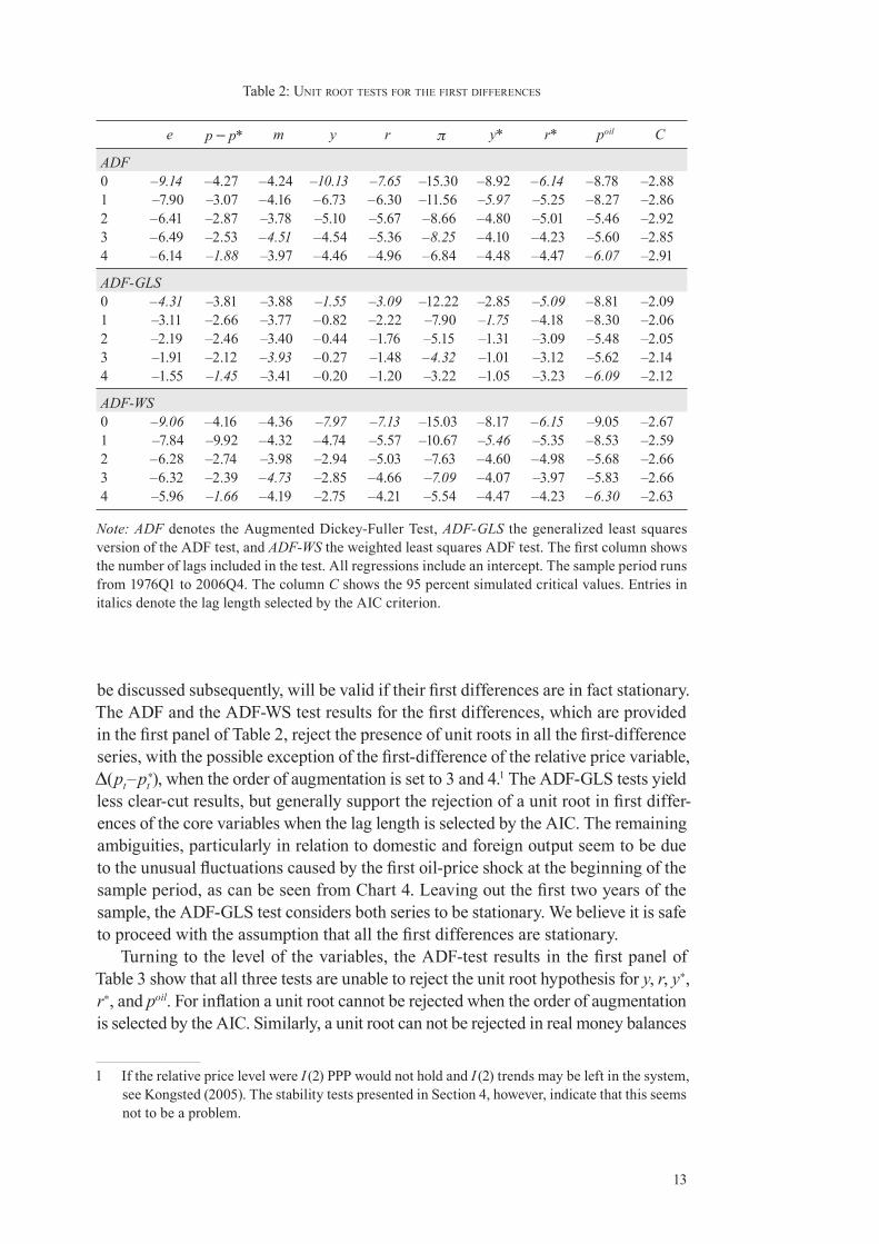
be discussed subsequently, will be valid if their fi rst differences are in fact stationary. The ADF and the ADF-WS test results for the fi rst differences, which are provided in the fi rst panel of Table 2, reject the presence of unit roots in all the fi rst-difference series, with the possible exception of the fi rst-difference of the relative price variable, Δ(pt – pt

∗), when the order of augmentation is set to 3 and 4.1 The ADF-GLS tests yield less clear-cut results, but generally support the rejection of a unit root in fi rst differ-ences of the core variables when the lag length is selected by the AIC. The remaining ambiguities, particularly in relation to domestic and foreign output seem to be due to the unusual fl uctuations caused by the fi rst oil-price shock at the beginning of the sample period, as can be seen from Chart 4. Leaving out the fi rst two years of the sample, the ADF-GLS test considers both series to be stationary. We believe it is safe to proceed with the assumption that all the fi rst differences are stationary.

Turning to the level of the variables, the ADF-test results in the fi rst panel of Table 3 show that all three tests are unable to reject the unit root hypothesis for y, r, y∗, r∗, and poil. For infl ation a unit root cannot be rejected when the order of augmentation is selected by the AIC. Similarly, a unit root can not be rejected in real money balances

1 If the relative price level were I (2) PPP would not hold and I (2) trends may be left in the system, see Kongsted (2005). The stability tests presented in Section 4, however, indicate that this seems not to be a problem.

Table 2: UNIT ROOT TESTS FOR THE FIRST DIFFERENCES

e p − p* m y r π y* r* poil C

ADF0 –9.14 –4.27 –4.24 –10.13 –7.65 –15.30 –8.92 –6.14 –8.78 –2.881 –7.90 –3.07 –4.16 –6.73 –6.30 –11.56 –5.97 –5.25 –8.27 –2.862 –6.41 –2.87 –3.78 –5.10 –5.67 –8.66 –4.80 –5.01 –5.46 –2.923 –6.49 –2.53 –4.51 –4.54 –5.36 –8.25 –4.10 –4.23 –5.60 –2.854 –6.14 –1.88 –3.97 –4.46 –4.96 –6.84 –4.48 –4.47 –6.07 –2.91

ADF-GLS0 –4.31 –3.81 –3.88 –1.55 –3.09 –12.22 –2.85 –5.09 –8.81 –2.091 –3.11 –2.66 –3.77 –0.82 –2.22 –7.90 –1.75 –4.18 –8.30 –2.062 –2.19 –2.46 –3.40 –0.44 –1.76 –5.15 –1.31 –3.09 –5.48 –2.053 –1.91 –2.12 –3.93 –0.27 –1.48 –4.32 –1.01 –3.12 –5.62 –2.144 –1.55 –1.45 –3.41 –0.20 –1.20 –3.22 –1.05 –3.23 –6.09 –2.12

ADF-WS0 –9.06 –4.16 –4.36 –7.97 –7.13 –15.03 –8.17 –6.15 –9.05 –2.671 –7.84 –9.92 –4.32 –4.74 –5.57 –10.67 –5.46 –5.35 –8.53 –2.592 –6.28 –2.74 –3.98 –2.94 –5.03 –7.63 –4.60 –4.98 –5.68 –2.663 –6.32 –2.39 –4.73 –2.85 –4.66 –7.09 –4.07 –3.97 –5.83 –2.664 –5.96 –1.66 –4.19 –2.75 –4.21 –5.54 –4.47 –4.23 –6.30 –2.63

Note: ADF denotes the Augmented Dickey-Fuller Test, ADF-GLS the generalized least squares version of the ADF test, and ADF-WS the weighted least squares ADF test. The fi rst column shows the number of lags included in the test. All regressions include an intercept. The sample period runs from 1976Q1 to 2006Q4. The column C shows the 95 percent simulated critical values. Entries in italics denote the lag length selected by the AIC criterion.

14

when the augmentation order of the underlying ADF regression is selected by the AIC, but the opposite result is obtained when ADF-GLS and the ADF-WS tests are used. The exchange rate, et, and relative price variable, pt – pt

∗, are also regarded as trend stationary by the ADF test but not by the ADF-GLS and the ADF-WS tests. Overall, however, it seems reasonable to regard all the series under consideration approximately as I (1) variables.

3. System approach: econometric methodology

The structural cointegrating VAR strategy starts with an explicit formulation of the long-run relationships between the variables in the model, derived from macr-oeconomic theory. These long-run relations are then incorporated in an otherwise unrestricted VAR. The cointegrating VAR embeds the structural long-run relations as the steady-state solutions while the short-run dynamics, about which economic theory in general is silent, is estimated from the data without restrictions. This seems a sensible strategy for the analysis of the long-run relations, but for forecasting it might also be desirable to restrict the short-run coeffi cients.

Table 3: UNIT ROOT TESTS FOR THE LEVELS

e p − p* m y r π y* r* poil T CADF0 –3.44 –9.21 –1.33 –1.94 –1.63 –4.63 –2.30 –1.11 –1.59 –3.50 –2.881 –4.04 –5.19 –3.45 –2.17 –2.45 –3.45 –2.36 –2.16 –2.23 –3.47 –2.862 –3.78 –4.51 –3.41 –2.45 –2.50 –2.77 –2.47 –2.24 –1.75 –3.51 –2.923 –3.85 –4.55 –3.66 –2.87 –2.45 –2.64 –3.58 –2.16 –2.32 –3.51 –2.854 –3.54 –4.44 –2.98 –3.04 –2.39 –2.30 –2.72 –2.45 –1.98 –3.41 –2.91

ADF-GLS0 –1.50 0.39 –1.20 –1.76 –0.84 –1.59 –0.90 –0.69 –1.57 –3.02 –2.091 –1.92 –0.51 –3.29 –1.93 –1.37 –1.07 –1.19 –1.52 –2.11 –2.91 –2.062 –1.70 –0.84 –3.24 –2.16 –1.37 –0.72 –1.42 –1.57 –1.70 –2.94 –2.053 –1.72 –0.89 –3.45 –2.54 –1.31 –0.63 –1.59 –1.48 –2.16 –2.93 –2.144 –1.43 –1.04 –2.81 –2.68 –1.24 –0.42 –1.74 –1.85 –1.87 –2.97 –2.12

ADF-WS0 –1.81 3.77 –1.33 –1.98 –1.56 –4.13 –0.94 –1.24 –1.62 –3.26 –2.671 –2.55 0.42 –3.67 –2.30 –2.32 –3.01 –1.46 –2.24 –2.27 –3.23 –2.592 –2.24 –0.40 –3.62 –2.55 –2.40 –2.43 –1.83 –2.25 –1.80 –3.27 –2.663 –2.38 –0.49 –3.84 –2.91 –2.34 –2.43 –2.01 –2.15 –2.36 –3.23 –2.664 –1.90 –0.71 –3.20 –3.09 –2.28 –2.05 –2.23 –2.46 2.03 –3.29 –2.63

Note: ADF denotes the Augmented Dickey-Fuller Test, ADF-GLS the generalized least squares ver-sion of the ADF test, and ADF-WS the weighted least squares ADF test. The fi rst column shows the number of lags included in the test. The regressions include a trend and an intercept for e, p − p*, m, y, y* and poil, and an intercept only for r, π, and r*. The sample period runs from 1976Q1 to 2006Q4. The column T gives the 95 percent simulated critical values for the test with intercept and trend, the column C the 95 percent simulated critical values for the test including an intercept only. Entries in italics denote the lag length selected by the AIC criterion.

15

In error-correction form the model can be written as

1

1 0 1=1

= ,p

t t i t i ti

tΔ Π Γ Δ−

− −− + + + +∑z z z a a u (1)

where *= ( , )t t t′′ ′z x x consists of a mx × 1 vector of endogenous variables, xt , and a

mx* × 1 vector of exogenous variables, x∗t, with mx + mx* = m. The matrix Π is a m × m

matrix of long-run multipliers and the matrices 1=1{ }p

i iΓ − summarise the short-run responses. The error term, ut, is distributed i.i.d.(0,Σ); a0 denotes a vector of con-stants and a1 a vector of trend coeffi cients. To partition the system into a conditional model for the endogenous variables, Δxt , and a marginal model for the exogenous variables, Δx∗

t, the parameter matrices and vectors Π, Γi, a0, a1 and the error term ut

are partitioned con form ably with *= ( , )t t t′′ ′z x x as Π' = (Π'x ,Π'x* ), Γi = (Γ'xi ,Γ'x*i ),

i = 1,…,p – 1, a0 = (a'x0 ,a'x*0 ), a1 = (a'x1 ,a'x*1 ), and ut = (u'xt ,u'x*t ). The variance matrix of ut can be written as

*

* * *

= ,xx xx

x x x x

Σ ΣΣ

Σ Σ

⎛ ⎞⎜ ⎟⎝ ⎠

so that

uxt = Σxx*Σ–1x*x*ux*t + υt,

where υt ~ i.i.d.(0, Σxx – Σxx*Σ–1x*x*Σx*x) is uncorrelated with ux*t by construction. For the

Swiss economy it is reasonable to assume that x∗t variables are weakly exogenous

so that Πx* = 0. This means that the information available from the model for Δx∗t

is redundant for effi cient estimation of the parameters of the conditional model for Δxt. The restrictions Πx* = 0 also imply that the variables x∗

t are I (1) and not cointegrated. If the x∗

t variables are cointegrated the cointegration test applied to the conditional model needs to be modifi ed. Although, to our knowledge a formal statistical analysis of this case is not yet available, our preliminary analysis suggests that the effective number of weakly exogenous variables used in testing for cointe-gartion based on the conditional model should be equal to the number of weakly exogenous variables, mx* minus the number of cointegration relations amongst the exogenous variables, say r∗. In the applications to follow we found that there exists one cointegration relation amongst the three weakly exogenous variables in the Swiss model.2 Therefore, to account for this we also report simulated critical values for the cointegration test in Table 5 that assume the existence of two (instead of three) exogenous I (1) variables.

2 To test for cointegration among the exogenous variables we estimated a system including two lags of foreign output, the foreign interest rate and the oil price as well as an unrestricted constant and a restricted trend. Neither the λ-max nor the trace test could reject the existence of a single cointegrating vector at the 10 percent level of signifi cance.

16

The system then can be written as a conditional model for the endogenous variables,

1

1 0 1=1

= ,p

t x t t i t i ti

tΔ Π ΛΔ Ψ Δ υx z x z c c−

∗− −− + + + + +∑ (2)

and the marginal model for the exogenous variables (assuming that x∗t variables are

not cointegrated)

1

* *0 *=1

= ,p

t x i t i x x ti

Δ Γ Δ−

∗− + +∑x z a u (3)

where Λ ≡ Σxx* Σ

−1x*x* , Ψi ≡ Γxi − Σxx* Σ

−1x*x* Γx*i , i = 1, …, p − 1,

c0 ≡ ax0 − Σxx* Σ−1x*x* ax0 and c1 ≡ ax1 − Σxx* Σ

−1x*x* ax*1 ,

see Garratt et al. (2006, p. 138).

If the model includes an unrestricted linear trend, in general there will be quadratic trends in the level of the variables when the model contains unit roots. To avoid this, the trend coeffi cients are restricted such that

c1 = Πxγ,

where γ is an m × 1 vector of free coeffi cients, see Pesaran, Shin and Smith (2000) and Garratt et al. (2006). The nature of the restrictions on c1 depends on the rank of Πx. In the case where Πx is full rank, c1 is unrestricted, whilst it is restricted to be equal to 0 when the rank of Πx is zero. Under the restricted trend coeffi cients the above VECM can be written as

[ ]1

1 0=1

= ( 1) ,p

t x t t i t i ti

tΔ Π γ ΛΔ Ψ Δ υx z x z c�−

∗− −− − − + + + +∑

where

0 0= .xΠ γ+c c�

Note that c̃0 remains unrestricted since c0 is not restricted.

17

4. Empirical results

4.1 Lag lengths and deterministic components

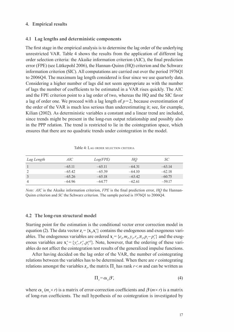
The fi rst stage in the empirical analysis is to determine the lag order of the underlying unrestricted VAR. Table 4 shows the results from the application of different lag order selection criteria: the Akaike information criterion (AIC), the fi nal prediction error (FPE) (see Lütkepohl 2006), the Hannan-Quinn (HQ) criterion and the Schwarz information criterion (SIC). All computations are carried out over the period 1976Q1 to 2006Q4. The maximum lag length considered is four since we use quarterly data. Considering a higher number of lags did not seem appropriate as with the number of lags the number of coeffi cients to be estimated in a VAR rises quickly. The AIC and the FPE criterion point to a lag order of two, whereas the HQ and the SIC favor a lag of order one. We proceed with a lag length of p = 2, because overestimation of the order of the VAR is much less serious than underestimating it; see, for example, Kilian (2002). As deterministic variables a constant and a linear trend are included, since trends might be present in the long-run output relationship and possibly also in the PPP relation. The trend is restricted to lie in the cointegration space, which ensures that there are no quadratic trends under cointegration in the model.

Table 4: LAG ORDER SELECTION CRITERIA

Lag Length AIC Log(FPE) HQ SC

1 –65.11 –65.11 –64.31 –63.142 –65.42 –65.39 –64.10 –62.183 –65.26 –65.18 –63.42 –60.754 –64.96 –64.77 –62.61 –59.17

Note: AIC is the Akaike information criterion, FPE is the fi nal prediction error, HQ the Hannan-Quinn criterion and SC the Schwarz criterion. The sample period is 1976Q1 to 2006Q4.

4.2 The long-run structural model

Starting point for the estimation is the conditional vector error correction model in equation (2). The data vector zt = {xt,xt

∗} contains the endogenous and exogenous vari-ables. The endogenous variables are ordered xt = {et, mt, yt, rt, πt, pt − pt

∗} and the exog-enous variables are xt

∗ = {yt∗, rt

∗, ptoil}. Note, however, that the ordering of these vari-

ables do not affect the cointegration test results of the generalized impulse functions.After having decided on the lag order of the VAR, the number of cointegrating

relations between the variables has to be determined. When there are r cointegrating relations amongst the variables zt, the matrix Πx has rank r < m and can be written as

Πx = αx β', (4)

where αx (mx × r) is a matrix of error-correction coeffi cients and β (m × r) is a matrix of long-run coeffi cients. The null hypothesis of no cointegration is investigated by

18

testing the rank of Πx. Table 5 shows the eigenvalues as well as the λ-max and the trace statistic together with their simulated critical values.

Table 5: COINTEGRATION TESTS

Rank Eigenvalue Trace CV3 90% CV2 90% λ-max CV3 90% CV2 90%

0 0.534 286.11 174.50 156.44 94.76 58.77 53.771 0.432 191.35 132.27 117.57 70.16 50.50 46.132 0.319 121.19 95.96 84.49 47.56 43.27 38.963 0.235 73.68 66.55 57.49 33.27 35.90 32.114 0.202 40.36 41.61 34.38 28.01 28.38 24.505 0.095 12.35 19.71 16.57 12.35 19.71 16.57

Note: The sample period is 1976Q1 to 2006Q4. CV3 (CV2) denotes the 90 percent simulated critical value that assume the presence of three (two) exogenous I (1) variables. Critical values are simulated with 1000 replications.

When using the simulated critical values that assume the presence of two exog-enous I (1) variables, both the trace test and the maximum eigenvalue (λ-max) test indicate the presence of fi ve cointegrating vectors at the 10% level of signifi cance. For completeness, we also report the critical values assuming three exogenous I (1) variables, which point to the same conclusion though the test statistics stay slightly below their critical values for r = 5. Overall, r = 5 seems a sensible choice, particularly considering that the long-run economic theory also predicts the existence of fi ve long-run relations.

To exactly identify the long-run relations, r restrictions (including a normalisation restriction) must be imposed on each of the r cointegrating relations. The cointegrat-ing vectors obtained by exact identifi cation are not presented here, since they do not have an economic interpretation. We proceed to imposing economically meaningful overidentifying restrictions that are in accordance with theoretical priors. Falling back on the results from the sub-system ARDL models, we impose overidentifying restrictions on β such that PPP, money demand, the output gap between domestic and foreign output, uncovered interest rate parity between the domestic and foreign interest rate, and a modifi ed Fisher equation that we interpret as the monetary author-ity’s long run interest-rate rule are imposed:

10 11 1PPP: ( ) = ,t t t te p p b b t ξ∗− − + +

20 24 2MD: = ,t t t tm y b rβ ξ− + +

30 37 3GAP: = ,t t ty b yβ ξ∗+ +

40 4UIP: = ,t t tr r b ξ∗− +

50 55 5LIR: = .t t tr b β π ξ+ +

19

These fi ve long-run relations can be written compactly as

0 1= ,t t tz b b′ − −ξ β

where b0 = (b10, b20, b30, b40, b50) and b1 = (b11, 0, 0, 0, 0).We impose a unitary income elasticity of money demand since the estimated

coeffi cient was close to unity. By contrast, we do not impose a coeffi cient of unity on the infl ation rate in the modifi ed Fisher equation since the empirical evidence indicated that this restriction is strongly rejected.3 In addition, it turned out that the lower trend output growth in Switzerland compared to its trading partners is better modelled by allowing for a non-unit coeffi cient on the foreign output variable than by including a trend in the output relation (the likelihood ratio test statistic is 78.65 in the former case versus 84.45 in the latter). The total number of overidentifying restrictions is 21, with the overidentifi ed β-matrix given by

24

37

55

1 0 0 0 0 1 0 0 0

0 1 1 0 0 0 0 0

= 0 0 1 0 0 0 0 0 .

0 0 0 1 0 0 0 1 0

0 0 0 1 0 0 0 0

β

β

β

−⎛ ⎞⎜ ⎟−⎜ ⎟⎜ ⎟⎜ ⎟

−⎜ ⎟⎜ ⎟⎝ ⎠

β

The estimated coeffi cients, together with their bootstrapped 95 percent confi dence bounds, are shown in Table 6. The estimate of β24 is 22.29, which means that money demand has a negative interest elasticity as to be expected. Since analytical stand-ard errors are valid only asymptotically and may give a wrong impression of the coeffi cients’ signifi cance, we bootstrap confi dence bounds for all the estimated long run coeffi cients. The reported confi dence bounds are obtained by a non-parametric bootstrap with 1000 replications.4 The upper 95 percent confi dence bound for β24 is 30.28 and the lower 95 percent bound is 15.55, implying that the interest elasticity of money demand is signifi cantly negative. The coeffi cient on foreign output, β37 , has a 95 percent confi dence band of –0.72 to –0.65 and thus is signifi cantly differ-ent from minus unity. The estimate of the infl ation coeffi cient, β55, is –1.58, with a bootstrapped 95 percent confi dence band of –2.11 to –1.26. This means that the coef-fi cient is signifi cantly smaller than the theoretically expected value of minus unity. One possible interpretation of this coeffi cient is that the monetary authority tends to over-react to infl ation in a systematic manner, so that the interest rate is raised more than infl ation in the long run. The estimate of the trend coeffi cient in the PPP relation is signifi cantly negative with a point estimate of –0.0004 and a 95 percent confi dence bound in the range of –0.0001 to –0.0008.

3 With a unitary coeffi cient on the infl ation rate in the last equation, β55 = –1, the interest elasticity of money demand declines from –22.29 to –8.96 and the likelihood ratio statistic increases substantially from 76.65 to 88.71.

4 Using a parametric bootstrap gives almost identical results.

20

Table 6: ESTIMATES OF OVERIDENTIFIED COINTEGRATION VECTORS

Coeffi cient Point estimate Lower 95% bound Upper 95% boundβ24 22.29 15.55 30.28

β37 –0.69 –0.72 –0.65β55 –1.58 –2.11 –1.26β11 –0.0004 –0.0001 –0.0008

Note: The confi dence bounds are obtained by a non-parametric bootstrap with 1000 replications.

A likelihood ratio (LR) test of the 21 overidentifying restrictions gives a test sta-tistic of 78.65, which is asymptotically distributed as a χ2 variate with 21 degrees of freedom. But due to the tendency of the asymptotic distribution to over-reject, once again we obtain the critical values from a non-parametric bootstrap with 1000 replications. This gives a critical value for the LR test statistic of 57.90 for the 5 percent level of signifi cance and of 69.07 for the 1 percent signifi cance level, as compared to the LR test statistic of 78.65.5 The test therefore rejects the restrictions at conventional signifi cance levels (the p-value is 0.2 percent). One has to keep in mind, however, that only four coeffi cients are estimated freely whereas the others are fi xed at their theoretical values. The relatively short sample period could also be another consideration to bear in mind. Since we could not fi nd a single restriction that was responsible for the rejection, we decided to proceed with the restricted estimates as they are in line with the long-run theory, and meet a number of other statistical requirements. For example, as we shall see below, the persistence profi les of all the fi ve coinetgrating relations tend to zero reasonably fast, and the effects of shocks on the cointegrating relations eventually vanish. None of these results would have followed if there were important departures from cointergation in the fi ve long run relations being considered.6

To examine stability properties of the cointegrating relations we fi rst present time plots of these relations in Chart 8, corrected for the short-run dynamics. These suggest that the PPP relation is strongly error-correcting, indicating that PPP forms one of the long-run relations in the system. Some more pronounced deviations from equilibrium occur in the output-gap relation during the late 1990s when Switzerland experienced a decade of unusually low growth. Since 2002, however, this deviation seems to have been corrected.

Finally, we check the recursive stability of β by means of a Nyblom (1989) test.7 Since the introduction of the SNB’s new monetary policy framework could have led to a structural break, we choose 2000Q1 as the start date of recursive stability tests. The Nyblom test statistic is 14.28 against a bootstrapped critical value of 29.56. Stability of the cointegrating vectors thus cannot be rejected.

5 Critical values from a parametric bootstrap with 1000 replications are quite similar with 60.49 for the 5 percent level and 70.36 for the 1 percent level of signifi cance.

6 We also investigated systems with four cointegrating vectors that leave out one of the more contentious cointegrating relations, i.e., PPP or the output gap, at the time. The results remained basically unchanged, namely we fi nd a coeffi cient on the infl ation rate in the long-run interest rule that is signifi cantly smaller than minus unity and the restrictions are rejected.

7 See Hansen and Johansen (1999).

21

Chart 8: CORRECTED COINTEGRATING RELATIONS

75 80 85 90 95 00 05

×10–1

1.0

0.5

0.0

–0.5

–1.0

–1.5 75 80 85 90 95 00 05

×10–2

0.75

0.50

0.25

0.00

–0.25

–0.50

–0.75

–1.00

PPP UIP

75 80 85 90 95 00 05

×10–1

2.0

1.5

1.0

0.5

0.0

–0.5

–1.0

–1.5 75 80 85 90 95 00 05

×10–2

2.0

1.5

1.0

0.5

0.0

–0.5

–1.0

–1.5

–2.0

MD LIR

75 80 85 90 95 00 05

×10–2

3.0

2.0

1.0

0.0

–1.0

–2.0

–3.0

GAP

22

4.3 Error-correction equations

Table 7 shows the estimates of the reduced-form error correction equations and some diagnostic statistics. The deviations from the long-run relations (the equilibrium errors) enter in most equations with high levels of signifi cance. Deviations from PPP help explain the exchange rate, domestic output and the interest rate. Deviations from money demand enter signifi cantly the money demand equation, the infl ation equation and the price differential equation. The deviation of domestic from foreign output is signifi cant in the money, output and interest rate equation, while the deviation of the domestic from the foreign interest rate contains information for the change in the domestic interest rate and infl ation. The error correction term from the interest rate rule has an infl uence on the change in the exchange rate, infl ation and the price differential.

The R2 values of the different equations range from 0.21 for the output equation to 0.77 for the price differential equation. The infl ation equation also fi ts quite well with a R2 of 0.61 for the change in the infl ation rate. The diagnostic statistics indicate that some serial correlation is present in the output and the price differential equation. For these two equations also the test for functional form rejects. While this could be improved by including further lags, the size of the system makes this solution unattractive because the number of coffi cients would increase considerably. The hypothesis of homoskedasticity of errors cannot be rejected for the exchange rate, the money, the output and the infl ation equation. The test for normality, however, strongly rejects in the case of the equations for et and yt. Looking at the residuals which are displayed, together with the actual and fi tted values for each equation, in Charts 9 to 14, one sees that these equations show some large outliers, especially at the beginning of the sample for domestic output and in the early 1980s for the exchange rate. These departures from normality are unlikely to have signifi cant impacts on our main fi ndings, but they do provide warnings of poor forecasting performance for these variables in certain periods of high market volatility.

Overall, the system seems to perform well. In particular, none of the tests indicates misspecifi cation in the infl ation equation, which will be central in the forecasting excercises. Assenmacher-Wesche and Pesaran (2008) document that the root mean squared forecast errors for output and infl ation from this model compare well to a broad range of similar models when estimated over an observation window starting in 1974 or later.

4.4 Generalized impulse responses and persistence profi les

The standard tool for the analysis of interactions and dynamics is the impulse response function, which considers the effects of a typical shock, usually one standard error, on the time path of the variables of the model. These shocks can be to observables, e.g., the oil price or interest rate, or to unobservables such technology or monetary policy variables. Shocks to observables can be calculated directly using Generalized Impulse Response Functions, GIRFs, introduced in Koop et al. (1996) and discussed in more detail in Pesaran and Shin (1998). See also Garratt et al. (2006, Chapter 6). The use of GIRF’s does not require any identifying assumptions and use the estimated error covariances to allow for the contemporaneous linkages that have

23

Table 7: REDUCED-FORM ERROR CORRECTION EQUATIONS

Equation Δet Δmt Δyt Δrt Δπt Δ( pt − p*t )

ξ̂1,t−1–0.190*

(0.070)–0.064(0.040)

0.054*

(0.022)0.018*

(0.004)–0.008(0.009)

0.013(0.010)

ξ̂2,t−10.035

(0.035)–0.063*

(0.020)0.016

(0.011)0.001

(0.002)0.016*

(0.005)0.013*

(0.005)

ξ̂3,t−1–0.040(0.167)

–0.194*

(0.094)–0.160*

(0.053)0.032*

(0.010)0.030

(0.022)–0.014(0.023)

ξ̂4,t−1–2.803(1.472)

1.369(0.831)

0.007(0.469)

–0.342*

(0.090)–0.404*

(0.193)0.269

(0.205)

ξ̂5,t−11.974*

(0.679)–0.566(0.383)

–0.169(0.216)

0.009(0.042)

0.564*

(0.089)0.222*

(0.094)

Δet−10.387*

(0.106)–0.132*

(0.060)0.006

(0.034)0.006

(0.006)0.043*

(0.014)0.033*

(0.015)

Δmt−1–0.106(0.132)

0.485*

(0.074)–0.008(0.042)

0.018*

(0.008)0.004

(0.017)0.015

(0.018)

Δyt−10.234

(0.306)–0.095(0.171)

–0.153(0.097)

0.036(0.019)

–0.003(0.040)

0.053(0.043)

Δrt−1–4.454*

(1.597)–0.560(0.902)

–0.037(0.509)

0.110(0.098)

–1.051*

(0.209)–1.328*

(0.222)

Δπt−1–0.674(0.581)

0.126(0.328)

–0.018(0.185)

–0.009(0.036)

–0.099(0.076)

–0.147(0.081)

Δ(pt−1 − p*t−1)2.396*

(0.809)–0.290(0.457)

–0.414(0.258)

0.027(0.049)

0.073(0.106)

0.575*

(0.113)

Δy*t–0.263(0.404)

–0.195(0.228)

0.514*

(0.129)0.018

(0.025)–0.037(0.053)

–0.030(0.056)

Δy*t−1–0.490(0.408)

–0.127(0.230)

0.134(0.130)

0.024(0.025)

–0.019(0.053)

–0.114*

(0.057)

Δr*t5.835*

(1.898)–5.198*

(1.072)1.603*

(0.605)0.837*

(0.116)1.057*

(0.248)0.744*

(0.264)

Δr*t−11.060

(2.546)–0.222(1.437)

0.279(0.811)

0.225(0.156)

0.444(0.333)

0.389(0.354)

Δpoilt

–0.007(0.015)

–0.020*(0.008)

–0.001(0.005)

0.001(0.001)

0.010*

(0.002)–0.003(0.002)

Δpoilt−1

0.026(0.017)

–0.005(0.010)

–0.001(0.005)

–0.001(0.001)

0.003(0.002)

0.004(0.002)

R2 0.210 0.756 0.307 0.577 0.614 0.768SC: χ2(4) 2.718 4.706 10.60 3.067 7.164 13.14FF: χ2(1) 1.434 1.068 4.071 1.151 0.001 7.332N: χ2(2) 94.57 1.197 61.86 3.600 3.747 0.315HS: χ2(1) 0.292 0.529 0.619 4.247 1.825 5.764

Note: The error correction terms, ξi, are defi ned on page 19. An asterisk denotes signifi cance at the 5 percent level. SC is a test for serial correlation, FF a test for functional form, N a test for normality and HS a test for heteroscedasticity. Critical values are 3.84 for χ2(1), 5.99 for χ2(2) and 9.49 for χ2(4). Constant not shown. The sample period is 1976Q1 to 2006Q4.

24

Chart 9: EXCHANGE RATE EQUATION

75 80 85 90 95 00 05

×10–1

0.75

0.50

0.25

0.00

–0.25

–0.50

–0.75

–1.00

–1.25 75 80 85 90 95 00 05

×10–1

0.6

0.4

0.2

0.0

–0.2

–0.4

–0.6

–0.8

–1.0

Actual and fitted Residuals

Chart 10: REAL MONEY EQUATION

75 80 85 90 95 00 05

×10–2

8.0

6.0

4.0

2.0

0.0

–2.0

–4.0

–6.0

–8.0 75 80 85 90 95 00 05

×10–2

3.0

2.0

1.0

0.0

–1.0

–2.0

–3.0


Chart 11: REAL OUTPUT EQUATION

75 80 85 90 95 00 05

×10–2

3.0

2.0

1.0

0.0

–1.0

–2.0 75 80 85 90 95 00 05

×10–2

3.0

2.0

1.0

0.0

–1.0

–2.0


25

Chart 12: INTEREST RATE EQUATION

75 80 85 90 95 00 05

×10–3

8.0

6.0

4.0

2.0

0.0

–2.0

–4.0

–6.0

–8.0 75 80 85 90 95 00 05

×10–3

4.0

3.0

2.0

1.0

0.0

–1.0

–2.0

–3.0

–4.0


Chart 13: INFLATION EQUATION

75 80 85 90 95 00 05

×10–2

1.5

1.0

0.5

0.0

–0.5

–1.0

–1.5 75 80 85 90 95 00 05

×10–3

8.0

6.0

4.0

2.0

0.0

–2.0

–4.0

–6.0


Chart 14: RELATIVE PRICE LEVEL EQUATION

75 80 85 90 95 00 05

×10–2

1.0

0.5

0.0

–0.5

–1.0

–1.5

–2.0

–2.5 75 80 85 90 95 00 05

×10–3

8.0

6.0

4.0

2.0

0.0

–2.0

–4.0

–6.0


26

prevailed between shocks historically. The effect of the shock to the observable on the other variables is of considerable interest in itself and should certainly be the fi rst stage of any analysis. It can be interpreted as the effect on the variables in the model of an intercept adjustment to the particular equation, e.g., the oil price or interest rate equation. However, for some purposes, we may wish to know where the shocks to observables come from. For interest rates we may wish to decompose the observable shock to the interest rate into a domestic monetary policy shock, a foreign monetary policy shock and a residual shock. However, to decompose the observable shock into its unobserved components requires more information which are often supplied by the economic theory of the short run. In what follows we focus on the response of the system to observable shocks and for this purpose use GIRF’s that are invariant to the ordering of the variables in the VAR.

The analysis of the dynamic properties of a system including exogenous I (1) variables requires the conditional model for Δxt in equation (2) together with the marginal model for Δx∗

t in equation (3). Specifi cation of the marginal model for Δx∗t

is necessary since the dynamic properties of the system have to accommodate the infl uence of the processes driving the exogenous variables. In other words, one needs to take into account the possibility that changes in one variable may have an impact on the exogenous variables and that these effects will continue and interact over time. For the marginal model, we chose a lag length of one. The full system is written as

1

1 0 1=1

= ,p

t t i t i ti

tΔ Γ Δ−

− −′− + + + +∑z z z a a Hαβ ζ (5)

where

* 0 *0 10 1

* *0

= , = , = , = ,i x i xxi

x i x

Ψ ΛΨ ΛΓ

Ψ

c a ca a

a0 0+ +⎛ ⎞ ⎛ ⎞⎛ ⎞ ⎛ ⎞

⎜ ⎟ ⎜ ⎟⎜ ⎟ ⎜ ⎟⎝ ⎠ ⎝ ⎠⎝ ⎠ ⎝ ⎠

αα

* * * *

= , = , ( ) = = ,t mxt t

x t mx x x

Cov ννζζ

υ Λ ΣΣ

Σ

I 0H

u 0 I 0⎛ ⎞ ⎛ ⎞ ⎛ ⎞⎜ ⎟ ⎜ ⎟ ⎜ ⎟⎝ ⎠ ⎝ ⎠ ⎝ ⎠

ζ ζ

c1 is restricted as before, and β is defi ned as in equation (4).Equation (5) can be rewritten as

0 1=1

= ,p

t i t i ti

tΦ − + + +∑z z a a Hζ (6)

where Φ1 = Im − αβ' + Γi , Φi = Γi − Γi−1 , i = 2, …, p − 1, Φp = −Γp−1. The generalized impulse responses are derived from the moving-average representation of equation (6),

0 1= ( )( ),t tL tΔ + +z C a a Hζwhere

=0

( ) = = (1) (1 ) ( ),jj

j

L L L L∞

∗+ −∑C C C C

=0 = 1

( ) = , and = ,jj j i

j i j

L L∞ ∞

∗ ∗ ∗

+

−∑ ∑C C C C

27

1 1 2 2= ... , for = 2,3,...,i i i p i p iΦ Φ Φ− − −+ + +C C C C (7)

0 1 1and = , = , and = 0, for 0.m m i iΦ − <C I C I C

Cumulating forward one obtains the level moving average representation,

0 0 0=1

= (1) ( ) ( ),t

t j tj

t L∗+ + + −∑z z b C H C Hζ ζ ζ

where b0 = C(1)a0 + C*(1)a1 and C(1)Πγ = 0 with γ being an arbitrary m × 1 vector of fi xed constants. The latter relation applies because the trend coeffi cients are restricted to lie in the cointegrating space.

We denote the generalized impulse response function (GIRF) of zt+n = (x't+n, x*'t+n)' at horizon n to a unit change in the error, ζit, measured by one standard deviation,

,iiζσ , by

, 1 1( , : ) = ( | = , ) ( | ).i t n it ii t t n tn E Eζε ζ σ+ − + −−z z zg I I

The GIRF is defi ned by the point forecast of zt+n conditional on the information set Jt–1 = (xt–1, xt–2, …; x*

t–1, x*t–2, …) and the shock ζit, relative to the baseline conditional

forecast.While the ζit are serially uncorrelated, they are contemporaneously correlated.

Thus a shock to the ith error, ζit, in general will affect the other errors. Therefore, at the horizon n = 0 the effect of a unit shock to the ith element of ζt, is given by

,

,

1( , : ) = ( | = ) = ,i t it ii i

ii

n E ζ ζζ

ζ

ζ ζ σ Σσ

⎛ ⎞⎜ ⎟⎜ ⎟⎝ ⎠

H eg ζ ζ

where ζt is iid (0,Σζζ ) and ei is an mx × 1 selection vector of zeros except for its ith element, which is set to unity. This yields the predicted effects of the ith shock on the other errors based on the observed historical error correlations. The GIRF is then given by

�,

1( , : ) = , = 0,1,…, = 1,…, ,ni i

ii

n n i mζζ

ζ

ζ Σσ

z C H eg

where

�=0

= ,n

n jj∑C C

which can be computed from the estimated coeffi cients in equation (5).While the impulse responses show the effect of a shock to a particular variable,

the persistence profi le, as developed by Lee and Pesaran (1993) and Pesaran and Shin (1996), show the effects of system-wide shocks on the cointegrating relations. In the case of the cointegrating relations the effects of the shocks (irrespective of their sources) will eventually disappear. Therefore, the shape of the persistence profi les

28

provide valuable information on the speed of convergence of the cointegrating rela-tions towards equilibrium. The persistence profi le for a given cointegrating relation defi ned by the cointegrating vector β j in the case of a VECX* model is given by

� �

( , ) = , = 0,1, , = 1, , ,n nj j

jj j

h n n j rζζ

ζζ

Σ

Σ

′ ′ ′′ … …

′ ′C H H C

zH H

β ββ

β β

where β, � ,nC H and Σζζ are as defi ned above.The impulse response of the cointegrating relations to a shock in variable i is also

defi ned as

�,

1( , ,: ) = , = 0,1, , = 1, , .nj i j i

ii

n n i mζζ

ζ

ζ Σσ

′ ′ … …z C H eg β β

Since � = (1) = ,j j∞′ ′C C 0β β for j = 1, 2, …, r, ultimately the effects of shocks on the cointegrating relations will vanish.

Chart 15 shows the persistence profi le of a system-wide shock to the cointegrat-ing relations together with their bootstrapped 95 percent confi dence bands. For all relations we can see a quick return to equilibrium. The persistence profi les of the PPP relation and the money demand relation overshoot after the initial shock, but like the other cointegrating vectors, they return to equilibrium reasonably quickly. The half life of the shocks ranges from only about one quarter for the long-run interest rate rule to one and half year for the output gap relation.

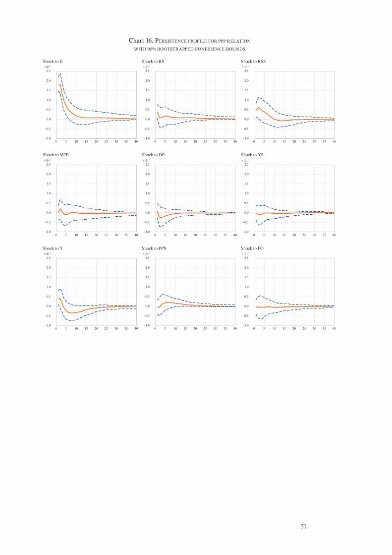
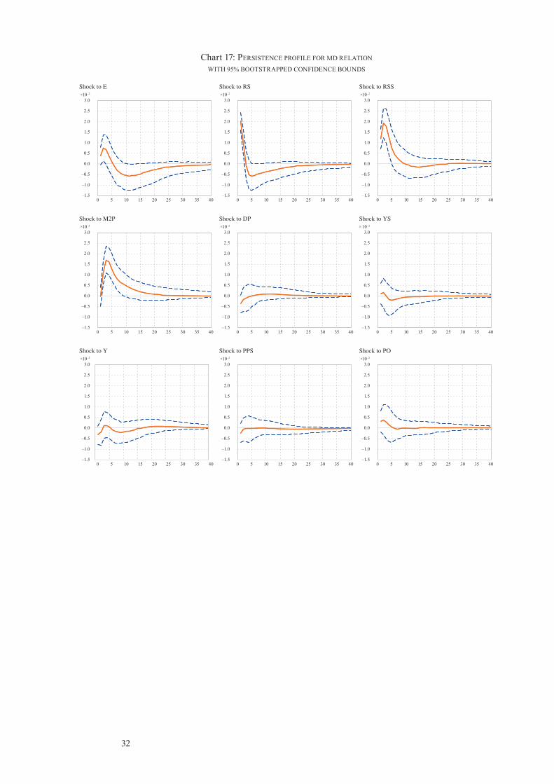
Charts 16 to 20 show the persistence profi le of the fi ve cointegrating relations to shocks to individual variables. These shocks can have only temporary effects. The cointegrating relations can be divided into relations combining macro variables, like PPP, money demand and the output relation, and relations linking fi nancial variables to each other, like the interest rate parity and the modifi ed Fisher equation. While shocks have a relatively large and long-lasting impact on r̀eal’ cointegrating relations, they die out quickly for the `fi nancial’ cointegrating relations. Exceptions are the effect of a shock to the domestic interest rate, which has only a short impact on the money demand relation, whereas shocks to the exchange rate, output and the foreign interest rate have a relatively long-lasting infl uence on the uncovered interest parity.

Finally, Charts 21 to 26 show the generalized impulse responses of the endogenous variables in the system to a one standard error shock to the various observables in the model. In a cointegrating VAR, shocks can have permanent effects on individual variables. The exchange rate and the relative price level are affected signifi cantly and permanently by shocks in these variables. The signifi cant responses of output, real money, the interest rate and infl ation to shocks in the exogenous variables dem-onstrate the importance of including these variables in a model for Switzerland as a small open economy. Charts 27 to 29 show the GIRFs of the exogenous variables. All the exogenous variables show a strong and persistent response to their own shocks.

29

5. Conclusions

This paper documents the development of a cointegrating VECX* model for the Swiss economy. In a cointegrating VAR model the implications of economic theory for the long-run relations between the variables in the model are combined with a data-driven approach to modeling the short-run dynamics. In the Swiss VECX* model we identify fi ve long-run relations. These are purchasing power parity, money demand, the uncovered interest parity relating domestic and foreign interest rates, a relation between domestic and foreign output, and a modifi ed Fisher equation that relates the domestic interest rate to the domestic infl ation rate.

The estimated model seems to have reasonable long-run properties and despite the fact that the overidentifying restrictions implied by the economic theory are rejected (at conventional levels of signifi cance), the economic importance of the rejections is unclear. A more satisfactory way to evaluate the model is to use it in forecasting and policy analysis. The former is addressed in Assenmacher-Wesche and Pesaran (2008). The latter will be addressed in future work.

Specifi cally, the current model could be extended into two directions. First, the short-run parameters could be estimated subject to restrictions using Bayesian priors. Since the VECX* model contains six endogenous and three exogenous variables, many coeffi cients in the model are imprecisely estimated. One can expect that Baye-sian estimation of the short-run coeffi cients will improve the forecasting performance of the model. Though there is a large literature on Bayesian estimation of unrestricted VAR models, Bayesian estimation of the short-run parameters in a cointegrating VAR has to deal with the restrictions implied by the long-run relations.

The second issue is the identifi cation of a short-run structure for the model. To be able to produce conditional forecasts given a specifi c path for the short-term interest rate, a monetary policy shock has to be identifi ed. To address this issue results in Pagan and Pesaran (2008) and in Pesaran and Smith (2006) that relate the VECX* model to New Keynesian DSGE models can be used.

30

Chart 15: PERSISTENCE PROFILES OF THE EFFECT OF A SYSTEM-WIDE SHOCK TO THE COINTEGRATING RELATIONS

WITH 95% BOOTSTRAPPED CONFIDENCE BOUNDS

75 80 85 90 95 00 05

1.75

1.50

1.25

1.00

0.75

0.5

0.25

0.0 75 80 85 90 95 00 05

1.2

1.0

0.8

0.6

0.4

0.2

0.0

PPP UIP

75 80 85 90 95 00 05

2.00

1.75

1.50

1.25

1.00

0.75

0.50

–0.25

0.00 75 80 85 90 95 00 05

1.00

0.75

0.50

0.25

0.00

MD LIR

75 80 85 90 95 00 05

1.4

1.2

1.0

0.8

0.6

0.4

0.2

0.0

GAP

31

Chart 16: PERSISTENCE PROFILE FOR PPP RELATION


×10–2

2.5

2.0

1.5

1.0

0.5

0.0

–0.5

–1.0

Shock to E

0 5 10 15 20 25 30 35 40

×10–2

2.5

2.0

1.5

1.0

0.5

0.0

–0.5

–1.0

Shock to M2P

0 5 10 15 20 25 30 35 40

×10–2

2.5

2.0

1.5

1.0

0.5

0.0

–0.5

–1.0

Shock to Y

0 5 10 15 20 25 30 35 40

×10–2

2.5

2.0

1.5

1.0

0.5

0.0

–0.5

–1.0

Shock to RS

0 5 10 15 20 25 30 35 40

×10–2

2.5

2.0

1.5

1.0

0.5

0.0

–0.5

–1.0

Shock to DP

0 5 10 15 20 25 30 35 40

×10–2

2.5

2.0

1.5

1.0

0.5

0.0

–0.5

–1.0

Shock to PPS

0 5 10 15 20 25 30 35 40

×10–2

2.5

2.0

1.5

1.0

0.5

0.0

–0.5

–1.0

Shock to RSS

0 5 10 15 20 25 30 35 40

×10–2

2.5

2.0

1.5

1.0

0.5

0.0

–0.5

–1.0

Shock to YS

0 5 10 15 20 25 30 35 40

×10–2

2.5

2.0

1.5

1.0

0.5

0.0

–0.5

–1.0

Shock to PO

0 5 10 15 20 25 30 35 40

32

Chart 17: PERSISTENCE PROFILE FOR MD RELATION


×10–2

3.0

2.5

2.0

1.5

1.0

0.5

0.0

–0.5

–1.0

–1.5

Shock to E

0 5 10 15 20 25 30 35 40

×10–2

3.0

2.5

2.0

1.5

1.0

0.5

0.0

–0.5

–1.0

–1.5

Shock to M2P

0 5 10 15 20 25 30 35 40

×10–2

3.0

2.5

2.0

1.5

1.0

0.5

0.0

–0.5

–1.0

–1.5

Shock to Y

0 5 10 15 20 25 30 35 40

×10–2

3.0

2.5

2.0

1.5

1.0

0.5

0.0

–0.5

–1.0

–1.5

Shock to RS

0 5 10 15 20 25 30 35 40

×10–2

3.0

2.5

2.0

1.5

1.0

0.5

0.0

–0.5

–1.0

–1.5

Shock to DP

0 5 10 15 20 25 30 35 40

×10–2

3.0

2.5

2.0

1.5

1.0

0.5

0.0

–0.5

–1.0

–1.5

Shock to PPS

0 5 10 15 20 25 30 35 40

×10–2

3.0

2.5

2.0

1.5

1.0

0.5

0.0

–0.5

–1.0

–1.5

Shock to RSS

0 5 10 15 20 25 30 35 40

× 10–2

3.0

2.5

2.0

1.5

1.0

0.5

0.0

–0.5

–1.0

–1.5

Shock to YS

0 5 10 15 20 25 30 35 40

×10–2

3.0

2.5

2.0

1.5

1.0

0.5

0.0

–0.5

–1.0

–1.5

Shock to PO

0 5 10 15 20 25 30 35 40

33

Chart 18: PERSISTENCE PROFILE FOR GAP RELATION


×10–3

7.5

6.0

4.5

3.0

1.5

0.0

–1.5

–3.0

Shock to E

0 5 10 15 20 25 30 35 40

×10–3

7.5

6.0

4.5

3.0

1.5

0.0

–1.5

–3.0

Shock to M2P

0 5 10 15 20 25 30 35 40

×10–3

7.5

6.0

4.5

3.0

1.5

0.0

–1.5

–3.0

Shock to Y

0 5 10 15 20 25 30 35 40

×10–3

7.5

6.0

4.5

3.0

1.5

0.0

–1.5

–3.0

Shock to RS

0 5 10 15 20 25 30 35 40

×10–3

7.5

6.0

4.5

3.0

1.5

0.0

–1.5

–3.0

Shock to DP

0 5 10 15 20 25 30 35 40

×10–3

7.5

6.0

4.5

3.0

1.5

0.0

–1.5

–3.0

Shock to PPS

0 5 10 15 20 25 30 35 40

×10–3

7.5

6.0

4.5

3.0

1.5

0.0

–1.5

–3.0

Shock to RSS

0 5 10 15 20 25 30 35 40

×10–3

7.5

6.0

4.5

3.0

1.5

0.0

–1.5

–3.0

Shock to YS

0 5 10 15 20 25 30 35 40

×10–3

7.5

6.0

4.5

3.0

1.5

0.0

–1.5

–3.0

Shock to PO

0 5 10 15 20 25 30 35 40

34

Chart 19: PERSISTENCE PROFILE FOR UIP RELATION


×10–3

1.50

1.25

1.00

0.75

0.50

0.25

0.00

–0.25

–0.50

–0.75

Shock to E

0 5 10 15 20 25 30 35 40

×10–3

1.50

1.25

1.00

0.75

0.50

0.25

0.00

–0.25

–0.50

–0.75

Shock to M2P

0 5 10 15 20 25 30 35 40

×10–3

1.50

1.25

1.00

0.75

0.50

0.25

0.00

–0.25

–0.50

–0.75

Shock to Y

0 5 10 15 20 25 30 35 40

×10–3

1.50

1.25

1.00

0.75

0.50

0.25

0.00

–0.25

–0.50

–0.75

Shock to RS

0 5 10 15 20 25 30 35 40

×10–3

1.50

1.25

1.00

0.75

0.50

0.25

0.00

–0.25

–0.50

–0.75

Shock to DP

0 5 10 15 20 25 30 35 40

×10–3

1.50

1.25

1.00

0.75

0.50

0.25

0.00

–0.25

–0.50

–0.75

Shock to PPS

0 5 10 15 20 25 30 35 40

×10–3

1.50

1.25

1.00

0.75

0.50

0.25

0.00

–0.25

–0.50

–0.75

Shock to RSS

0 5 10 15 20 25 30 35 40

×10–3

1.50

1.25

1.00

0.75

0.50

0.25

0.00

–0.25

–0.50

–0.75

Shock to YS

0 5 10 15 20 25 30 35 40

×10–3

1.50

1.25

1.00

0.75

0.50

0.25

0.00

–0.25

–0.50

–0.75

Shock to PO

0 5 10 15 20 25 30 35 40

35

Chart 20: PERSISTENCE PROFILE FOR LIR RELATION


×10–3

3.0

1.5

0.0

–1.5

–3.0

–4.5

Shock to E

0 5 10 15 20 25 30 35 40

×10–3

3.0

1.5

0.0

–1.5

–3.0

–4.5

Shock to M2P

0 5 10 15 20 25 30 35 40

×10–3

3.0

1.5

0.0

–1.5

–3.0

–4.5

Shock to Y

0 5 10 15 20 25 30 35 40

×10–3

3.0

1.5

0.0

–1.5

–3.0

–4.5

Shock to RS

0 5 10 15 20 25 30 35 40

×10–3

3.0

1.5

0.0

–1.5

–3.0

–4.5

Shock to DP

0 5 10 15 20 25 30 35 40

×10–3

3.0

1.5

0.0

–1.5

–3.0

–4.5

Shock to PPS

0 5 10 15 20 25 30 35 40

×10–3

3.0

1.5

0.0

–1.5

–3.0

–4.5

Shock to RSS

0 5 10 15 20 25 30 35 40

×10–3

3.0

1.5

0.0

–1.5

–3.0

–4.5

Shock to YS

0 5 10 15 20 25 30 35 40

×10–3

3.0

1.5

0.0

–1.5

–3.0

–4.5

Shock to PO

0 5 10 15 20 25 30 35 40

36

Chart 21: GENERALIZED IMPULSE RESPONSES FOR EXCHANGE RATE


×10–2

3.0

2.5

2.0

1.5

1.0

0.5

0.0

–0.5

–1.0

–1.5

Shock to E

0 5 10 15 20 25 30 35 40

×10–2

3.0

2.5

2.0

1.5

1.0

0.5

0.0

–0.5

–1.0

–1.5

Shock to M2P

0 5 10 15 20 25 30 35 40

×10–2

3.0

2.5

2.0

1.5

1.0

0.5

0.0

–0.5

–1.0

–1.5

Shock to Y

0 5 10 15 20 25 30 35 40

×10–2

3.0

2.5

2.0

1.5

1.0

0.5

0.0

–0.5

–1.0

–1.5

Shock to RS

0 5 10 15 20 25 30 35 40

×10–2

3.0

2.5

2.0

1.5

1.0

0.5

0.0

–0.5

–1.0

–1.5

Shock to DP

0 5 10 15 20 25 30 35 40

×10–2

3.0

2.5

2.0

1.5

1.0

0.5

0.0

–0.5

–1.0

–1.5

Shock to PPS

0 5 10 15 20 25 30 35 40

×10–2

3.0

2.5

2.0

1.5

1.0

0.5

0.0

–0.5

–1.0

–1.5

Shock to RSS

0 5 10 15 20 25 30 35 40

×10–2

3.0

2.5

2.0

1.5

1.0

0.5

0.0

–0.5

–1.0

–1.5

Shock to YS

0 5 10 15 20 25 30 35 40

×10–2

3.0

2.5

2.0

1.5

1.0

0.5

0.0

–0.5

–1.0

–1.5

Shock to PO

0 5 10 15 20 25 30 35 40

37

Chart 22: GENERALIZED IMPULSE RESPONSES FOR REAL M2


×10–2

3.0

1.5

0.0

–1.5

–3.0

–4.5

–6.0

Shock to E

0 5 10 15 20 25 30 35 40

×10–2

3.0

1.5

0.0

–1.5

–3.0

–4.5

–6.0

Shock to M2P

0 5 10 15 20 25 30 35 40

×10–2

3.0

1.5

0.0

–1.5

–3.0

–4.5

–6.0

Shock to Y

0 5 10 15 20 25 30 35 40

×10–2

3.0

1.5

0.0

–1.5

–3.0

–4.5

–6.0

Shock to RS

0 5 10 15 20 25 30 35 40

×10–2

3.0

1.5

0.0

–1.5

–3.0

–4.5

–6.0

Shock to DP

0 5 10 15 20 25 30 35 40

×10–2

3.0

1.5

0.0

–1.5

–3.0

–4.5

–6.0

Shock to PPS

0 5 10 15 20 25 30 35 40

×10–2

3.0

1.5

0.0

–1.5

–3.0

–4.5

–6.0

Shock to RSS

0 5 10 15 20 25 30 35 40

×10–2

3.0

1.5

0.0

–1.5

–3.0

–4.5

–6.0

Shock to YS

0 5 10 15 20 25 30 35 40

×10–2

3.0

1.5

0.0

–1.5

–3.0

–4.5

–6.0

Shock to PO

0 5 10 15 20 25 30 35 40

38

Chart 23: GENERALIZED IMPULSE RESPONSES FOR OUTPUT


×10–3

8

6

4

2

0

–2

–4

Shock to E

0 5 10 15 20 25 30 35 40

×10–3

8

6

4

2

0

–2

–4

Shock to M2P

0 5 10 15 20 25 30 35 40

×10–3

8

6

4

2

0

–2

–4

Shock to Y

0 5 10 15 20 25 30 35 40

×10–3

8

6

4

2

0

–2

–4

Shock to RS

0 5 10 15 20 25 30 35 40

×10–3

8

6

4

2

0

–2

–4

Shock to DP

0 5 10 15 20 25 30 35 40

×10–3

8

6

4

2

0

–2

–4

Shock to PPS

0 5 10 15 20 25 30 35 40

×10–3

8

6

4

2

0

–2

–4

Shock to RSS

0 5 10 15 20 25 30 35 40

×10–3

8

6

4

2

0

–2

–4

Shock to YS

0 5 10 15 20 25 30 35 40

×10–3

8

6

4

2

0

–2

–4

Shock to PO

0 5 10 15 20 25 30 35 40

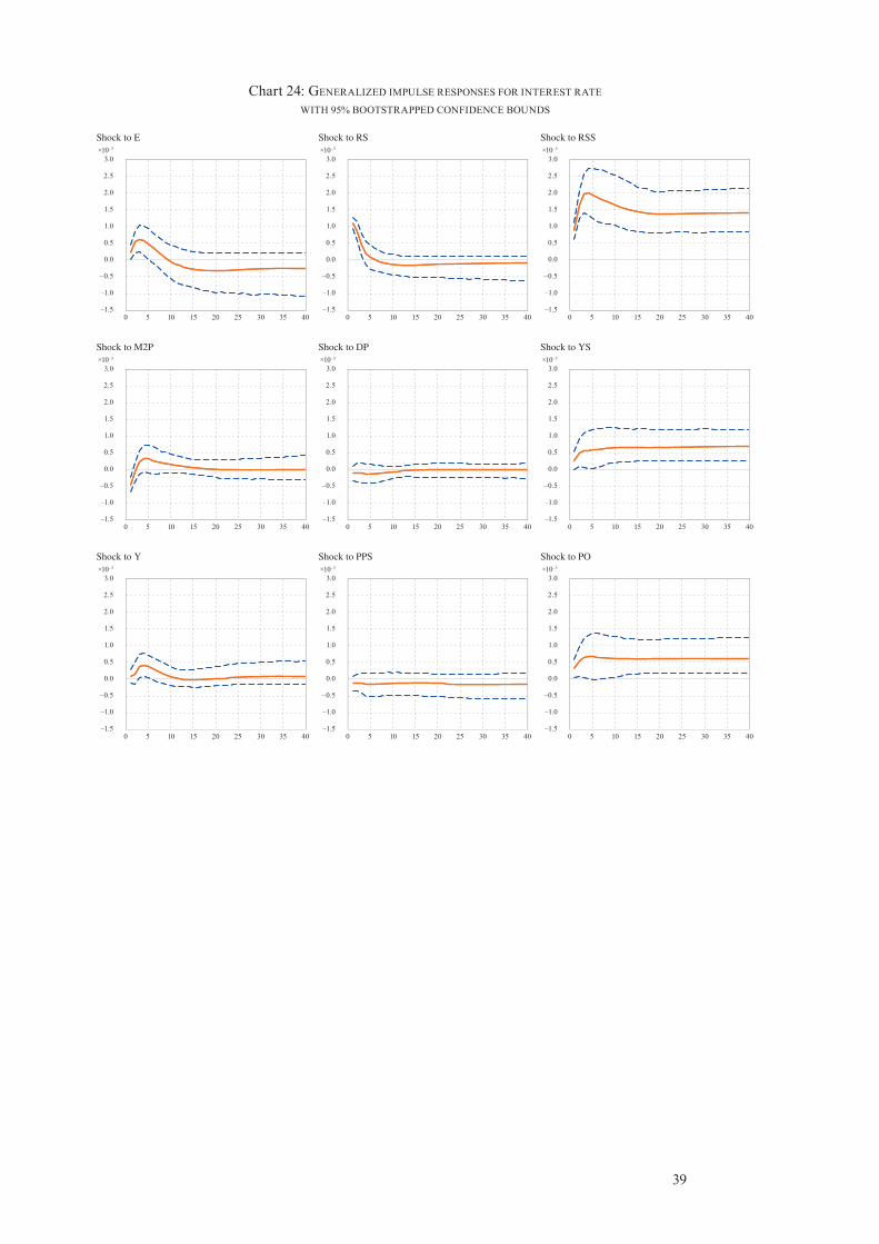
39

Chart 24: GENERALIZED IMPULSE RESPONSES FOR INTEREST RATE


×10–3

3.0

2.5

2.0

1.5

1.0

0.5

0.0

–0.5

–1.0

–1.5

Shock to E

0 5 10 15 20 25 30 35 40

×10–3

3.0

2.5

2.0

1.5

1.0

0.5

0.0

–0.5

–1.0

–1.5

Shock to M2P

0 5 10 15 20 25 30 35 40

×10–3

3.0

2.5

2.0

1.5

1.0

0.5

0.0

–0.5

–1.0

–1.5

Shock to Y

0 5 10 15 20 25 30 35 40

×10–3

3.0

2.5

2.0

1.5

1.0

0.5

0.0

–0.5

–1.0

–1.5

Shock to RS

0 5 10 15 20 25 30 35 40

×10–3

3.0

2.5

2.0

1.5

1.0

0.5

0.0

–0.5

–1.0

–1.5

Shock to DP

0 5 10 15 20 25 30 35 40

×10–3

3.0

2.5

2.0

1.5

1.0

0.5

0.0

–0.5

–1.0

–1.5

Shock to PPS

0 5 10 15 20 25 30 35 40

×10–3

3.0

2.5

2.0

1.5

1.0

0.5

0.0

–0.5

–1.0

–1.5

Shock to RSS

0 5 10 15 20 25 30 35 40

×10–3

3.0

2.5

2.0

1.5

1.0

0.5

0.0

–0.5

–1.0

–1.5

Shock to YS

0 5 10 15 20 25 30 35 40

×10–3

3.0

2.5

2.0

1.5

1.0

0.5

0.0

–0.5

–1.0

–1.5

Shock to PO

0 5 10 15 20 25 30 35 40

40

Chart 25: GENERALIZED IMPULSE RESPONSES FOR INFLATION


×10–3

3.0

2.5

2.0

1.5

1.0

0.5

0.0

–0.5

–1.0

–1.5

Shock to E

0 5 10 15 20 25 30 35 40

×10–3

3.0

2.5

2.0

1.5

1.0

0.5

0.0

–0.5

–1.0

–1.5

Shock to M2P

0 5 10 15 20 25 30 35 40

×10–3

3.0

2.5

2.0

1.5

1.0

0.5

0.0

–0.5

–1.0

–1.5

Shock to Y

0 5 10 15 20 25 30 35 40

×10–3

3.0

2.5

2.0

1.5

1.0

0.5

0.0

–0.5

–1.0

–1.5

Shock to RS

0 5 10 15 20 25 30 35 40

×10–3

3.0

2.5

2.0

1.5

1.0

0.5

0.0

–0.5

–1.0

–1.5

Shock to DP

0 5 10 15 20 25 30 35 40

×10–3

3.0

2.5

2.0

1.5

1.0

0.5

0.0

–0.5

–1.0

–1.5

Shock to PPS

0 5 10 15 20 25 30 35 40

×10–3

3.0

2.5

2.0

1.5

1.0

0.5

0.0

–0.5

–1.0

–1.5

Shock to RSS

0 5 10 15 20 25 30 35 40

×10–3

3.0

2.5

2.0

1.5

1.0

0.5

0.0

–0.5

–1.0

–1.5

Shock to YS

0 5 10 15 20 25 30 35 40

×10–3

3.0

2.5

2.0

1.5

1.0

0.5

0.0

–0.5

–1.0

–1.5

Shock to PO

0 5 10 15 20 25 30 35 40

41

Chart 26: GENERALIZED IMPULSE RESPONSES FOR RELATIVE PRICE LEVEL


×10–2

2.0

1.6

1.2

0.8

0.4

0.0

–0.4

–0.8

–1.2

Shock to E

0 5 10 15 20 25 30 35 40

×10–2

2.0

1.6

1.2

0.8

0.4

0.0

–0.4

–0.8

–1.2

Shock to M2P

0 5 10 15 20 25 30 35 40

×10–2

2.0

1.6

1.2

0.8

0.4

0.0

–0.4

–0.8

–1.2

Shock to Y

0 5 10 15 20 25 30 35 40

×10–2

2.0

1.6

1.2

0.8

0.4

0.0

–0.4

–0.8

–1.2

Shock to RS

0 5 10 15 20 25 30 35 40

×10–2

2.0

1.6

1.2

0.8

0.4

0.0

–0.4

–0.8

–1.2

Shock to DP

0 5 10 15 20 25 30 35 40

×10–2

2.0

1.6

1.2

0.8

0.4

0.0

–0.4

–0.8

–1.2

Shock to PPS

0 5 10 15 20 25 30 35 40

×10–2

2.0

1.6

1.2

0.8

0.4

0.0

–0.4

–0.8

–1.2

Shock to RSS

0 5 10 15 20 25 30 35 40

×10–2

2.0

1.6

1.2

0.8

0.4

0.0

–0.4

–0.8

–1.2

Shock to YS

0 5 10 15 20 25 30 35 40

×10–2

2.0

1.6

1.2

0.8

0.4

0.0

–0.4

–0.8

–1.2

Shock to PO

0 5 10 15 20 25 30 35 40

42

Chart 27: GENERALIZED IMPULSE RESPONSES FOR FOREIGN OUTPUT


×10–3

8

6

4

2

0

–2

–4

Shock to E

0 5 10 15 20 25 30 35 40

×10–3

8

6

4

2

0

–2

–4

Shock to M2P

0 5 10 15 20 25 30 35 40

×10–3

8

6

4

2

0

–2

–4

Shock to Y

0 5 10 15 20 25 30 35 40

×10–3

8

6

4

2

0

–2

–4

Shock to RS

0 5 10 15 20 25 30 35 40

×10–3

8

6

4

2

0

–2

–4

Shock to DP

0 5 10 15 20 25 30 35 40

×10–3

8

6

4

2

0

–2

–4

Shock to PPS

0 5 10 15 20 25 30 35 40

×10–3

8

6

4

2

0

–2

–4

Shock to RSS

0 5 10 15 20 25 30 35 40

×10–3

8

6

4

2

0

–2

–4

Shock to YS

0 5 10 15 20 25 30 35 40

×10–3

8

6

4

2

0

–2

–4

Shock to PO

0 5 10 15 20 25 30 35 40

43

Chart 28: GENERALIZED IMPULSE RESPONSES FOR FOREIGN INTEREST RATE


×10–3

2.5

2.0

1.5

1.0

0.5

0.0

–0.5

–1.0

–1.5

Shock to E

0 5 10 15 20 25 30 35 40

×10–3

2.5

2.0

1.5

1.0

0.5

0.0

–0.5

–1.0

–1.5

Shock to M2P

0 5 10 15 20 25 30 35 40

×10–3

2.5

2.0

1.5

1.0

0.5

0.0

–0.5

–1.0

–1.5

Shock to Y

0 5 10 15 20 25 30 35 40

×10–3

2.5

2.0

1.5

1.0

0.5

0.0

–0.5

–1.0

–1.5

Shock to RS

0 5 10 15 20 25 30 35 40

×10–3

2.5

2.0

1.5

1.0

0.5

0.0

–0.5

–1.0

–1.5

Shock to DP

0 5 10 15 20 25 30 35 40

×10–3

2.5

2.0

1.5

1.0

0.5

0.0

–0.5

–1.0

–1.5

Shock to PPS

0 5 10 15 20 25 30 35 40

×10–3

2.5

2.0

1.5

1.0

0.5

0.0

–0.5

–1.0

–1.5

Shock to RSS

0 5 10 15 20 25 30 35 40

×10–3

2.5

2.0

1.5

1.0

0.5

0.0

–0.5

–1.0

–1.5

Shock to YS

0 5 10 15 20 25 30 35 40

×10–3

2.5

2.0

1.5

1.0

0.5

0.0

–0.5

–1.0

–1.5

Shock to PO

0 5 10 15 20 25 30 35 40

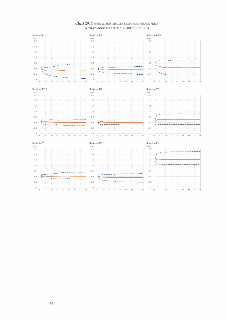
44

Chart 29: GENERALIZED IMPULSE RESPONSES FOR OIL PRICE


×10–1

2.5

2.0

1.5

1.0

0.5

0.0

–0.5

–1.0

Shock to E

0 5 10 15 20 25 30 35 40

×10–1

2.5

2.0

1.5

1.0

0.5

0.0

–0.5

–1.0

Shock to M2P

0 5 10 15 20 25 30 35 40

×10–1

2.5

2.0

1.5

1.0

0.5

0.0

–0.5

–1.0

Shock to Y

0 5 10 15 20 25 30 35 40

×10–1

2.5

2.0

1.5

1.0

0.5

0.0

–0.5

–1.0

Shock to RS

0 5 10 15 20 25 30 35 40

×10–1

2.5

2.0

1.5

1.0

0.5

0.0

–0.5

–1.0

Shock to DP

0 5 10 15 20 25 30 35 40

×10–1

2.5

2.0

1.5

1.0

0.5

0.0

–0.5

–1.0

Shock to PPS

0 5 10 15 20 25 30 35 40

×10–1

2.5

2.0

1.5

1.0

0.5

0.0

–0.5

–1.0

Shock to RSS

0 5 10 15 20 25 30 35 40

×10–1

2.5

2.0

1.5

1.0

0.5

0.0

–0.5

–1.0

Shock to YS

0 5 10 15 20 25 30 35 40

×10–1

2.5

2.0

1.5

1.0

0.5

0.0

–0.5

–1.0

Shock to PO

0 5 10 15 20 25 30 35 40

45

Appendix

Appendix: Sources and construction of data

Swiss data

All Swiss data are from the data base of the Swiss National Bank (SNB). The short-term interest rate is the end-of-month three-month London Interbank Offered Rate (3M LIBOR) for Swiss francs, denoted by R. The interest rate is expressed as 0.25ln(1 + R / 100), so that it matches the quarterly measure of the infl ation rate. The price level is the consumer price index (CPI) with the base of December 2005 = 100. Money is M2 in the defi nition of 1995, excluding Liechtenstein. Real money is M2 defl ated by the CPI. Output is the seasonally adjusted quarterly real gross domestic product (GDP) computed by the SECO (Secrétariat d’Etat à l’économie) from 1981 onward. Quarterly output estimates before 1981 were interpolated from the offi cial annual data by the SNB.

For the CPI an adjustment was made to overcome breaks due to new data collec-tion procedures at the Swiss Federal Statistical Offi ce. From 2000 on the CPI includes end-of-season sales. This introduces substantial seasonality into the sub-index for clothing and footwear, as can be seen in Chart A.1. In addition, the data collection had been shifted from the end of the month to the beginning of the month in January 2002, which introduces another break into the series. We adjust for these changes by shifting the series by one month backward between January 2000 and January 2002, the period indicated by the vertical lines in Chart A.1. The resulting missing value is fi lled by inserting the December 2001 value of the sub-index. The series is smoothed by computing a twelve-month backward moving average. The smoothed sub-index is added to the CPI without clothing and footwear, using the weight of this sub-index in the CPI. Chart A.2 shows the original and the adjusted CPI series. Though the weight of the clothing-and-footwear sub-index is less than 5 percent since 2000, it is clearly visible that the adjustment considerably reduces the seasonal variability of the infl ation rate since 2002.

Monthly data for real M2, the CPI and the 3M LIBOR are aggregated into quar-terly averages of monthly fi gures. Infl ation is the quarterly percent difference of the CPI.

Foreign data

The foreign price level, the exchange rate and foreign GDP are constructed using trade-weighted data from Switzerland’s 15 most important trading partners. These are (in the order of their importance) Germany, France, Italy, the United States, the United Kingdom, Austria, the Netherlands, Japan, Belgium, Spain, Sweden, Hongkong, China, Ireland and Denmark. Monthly trade data are from the Eidgenös-sische Zollverwaltung. Trade is defi ned as the sum of imports and exports from and to a specifi c country. The countries considered have an average share of at

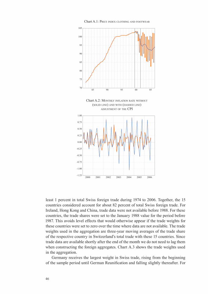
46

least 1 percent in total Swiss foreign trade during 1974 to 2006. Together, the 15 countries considered account for about 82 percent of total Swiss foreign trade. For Ireland, Hong Kong and China, trade data were not available before 1988. For these countries, the trade shares were set to the January 1988 value for the period before 1987. This avoids level effects that would otherwise appear if the trade weights for these countries were set to zero over the time where data are not available. The trade weights used in the aggregation are three-year moving averages of the trade share of the respective country in Switzerland’s total trade with these 15 countries. Since trade data are available shortly after the end of the month we do not need to lag them when constructing the foreign aggregates. Chart A.3 shows the trade weights used in the aggregation.

Germany receives the largest weight in Swiss trade, rising from the beginning of the sample period until German Reunifi cation and falling slightly thereafter. For

70

75

80

85

90

95

100

105

85 90 95 00 05

Chart A.1: PRICE INDEX CLOTHING AND FOOTWEAR

Chart A.2: MONTHLY INFLATION RATE WITHOUT (SOLID LINE) AND WITH (DASHED LINE)

ADJUSTMENT OF THE CPI

-1.25

-1.00

-0.75

-0.50

-0.25

0.00

0.25

0.50

0.75

1.00

2000 2001 2002 2003 2004 2005 2006

47

Chart A.3: TRADE WEIGHTS: LEVELS (SOLID LINE) AND PERCENTAGE CHANGE (DASHED LINE)

×10–1

4.0

3.5

3.0

2.5

2.0

1.5

1.0

0.5

0.0

Germany

75 80 85 90 95 00 05

×10–1

4.0

3.5

3.0

2.5

2.0

1.5

1.0

0.5

0.0

France

75 80 85 90 95 00 05

×10–1

4.0

3.5

3.0

2.5

2.0

1.5

1.0

0.5

0.0

Italy

75 80 85 90 95 00 05

×10–1

4.0

3.5

3.0

2.5

2.0

1.5

1.0

0.5

0.0

United States

75 80 85 90 95 00 05

×10–1

4.0

3.5

3.0

2.5

2.0

1.5

1.0

0.5

0.0

United Kingdom

75 80 85 90 95 00 05

×10–1

4.0

3.5

3.0

2.5

2.0

1.5

1.0

0.5

0.0

Austria

75 80 85 90 95 00 05

×10–1

4.0

3.5

3.0

2.5

2.0

1.5

1.0

0.5

0.0

Netherlands

75 80 85 90 95 00 05

×10–1

4.0

3.5

3.0

2.5

2.0

1.5

1.0

0.5

0.0

Japan

75 80 85 90 95 00 05

×10–1

4.0

3.5

3.0

2.5

2.0

1.5

1.0

0.5

0.0

Belgium

75 80 85 90 95 00 05

×10–1

4.0

3.5

3.0

2.5

2.0

1.5

1.0

0.5

0.0

Spain

75 80 85 90 95 00 05

×10–1

4.0

3.5

3.0

2.5

2.0

1.5

1.0

0.5

0.0

Sweden

75 80 85 90 95 00 05

×10–1

4.0

3.5

3.0

2.5

2.0

1.5

1.0

0.5

0.0

Denmark

75 80 85 90 95 00 05

×10–1

4.0

3.5

3.0

2.5

2.0

1.5

1.0

0.5

0.0

Hong Kong

75 80 85 90 95 00 05

×10–1

4.0

3.5

3.0

2.5

2.0

1.5

1.0

0.5

0.0

Canada

75 80 85 90 95 00 05

×10–1

4.0

3.5

3.0

2.5

2.0

1.5

1.0

0.5

0.0

Ireland

75 80 85 90 95 00 05

10

8

6

4

2

0

–2

–4

–6

10

8

6

4

2

0

–2

–4

–6

10

8

6

4

2

0

–2

–4

–6

10

8

6

4

2

0

–2

–4

–6

10

8

6

4

2

0

–2

–4

–6

10

8

6

4

2

0

–2

–4

–6

10

8

6

4

2

0

–2

–4

–6

10

8

6

4

2

0

–2

–4

–6

10

8

6

4

2

0

–2

–4

–6

10

8

6

4

2

0

–2

–4

–6

10

8

6

4

2

0

–2

–4

–6

10

8

6

4

2

0

–2

–4

–6

10

8

6

4

2

0

–2

–4

–6

10

8

6

4

2

0

–2

–4

–6

10

8

6

4

2

0

–2

–4

–6

48

most countries, trade shares have remained fairly constant over the sample period. In general, trade shares for the European countries have tended to fall, e.g., for France, the UK, Austria, Belgium, Sweden and Denmark. By contrast, trade with Spain, Ire-land and China has increased rapidly, though from very low levels. The fl uctuations in the exchange rate, particularly in the US dollar, are mirrored in the fl uctuation of the US trade share.

The foreign price level is the trade-weighted aggregate of the consumer price indices, and foreign GDP is the trade-weighted aggregate of the real GDP indices of the 15 main trading partners. The CPI and real GDP data are from the Main Eco-nomic Indicators data base of the OECD. Missing data have been supplemented with IFS and BIS data. For countries where the GDP data were not seasonally adjusted at the source, the X12 procedure was used to seasonally adjust the original series. When quarterly data were not available, annual data were interpolated.8 All GDP series were converted to an index with the base year 2000 and then aggregated using the three-year moving averages of the trade weights. This avoids the use of exchange rates to convert GDP into a common currency.9

In contrast to the foreign CPI and GDP, the foreign interest rate and the exchange rate are weighted averages of the three-month interest rate and the exchange rate in the euro area and the US only. This seems justifi ed considering the dominant role played by these two economies in the evolution of the fi nancial market intercon-nections of the Swiss economy and the rest of the world. The weights are shown in Chart A.4. While the EMU countries receive a share of about 82 percent, the US fi nancial variables account for about 10 percent of the total.

Before the existence of European Monetary Union, the euro area interest rate and exchange rate are proxied by a weighted average of the short-term interest rates and exchange rates of those countries among Switzerland’s 15 main trading partners that entered the EMU. After the transition to European monetary union, the exchange rate for the members of the European Monetary Union are replaced by the Euro exchange rate, converted with the offi cial conversion rates of the national currencies to the Euro at the start of the European Monetary Union in 1999. The foreign interest rates are from the BIS data base. Like the domestic interest rate, the foreign interest rate is expressed as 0.25ln(1 + R* / 100), where R* is the foreign interest rate per annum in percent.

The monthly series for the CPI, the interest rate and the exchange rate were aggre-gated with monthly trade weights and then transformed into quarterly averages.

8 This was the case for the Netherlands and Denmark until 1976, for Belgium until 1979, for Ireland and Hong Kong until 1985, and for China until 1999.

9 Though it might seem that using GDP indexes neglects the different size of Switzerland’s trading partners, it only matters up to a constant if the aggregation weights do not change over time.

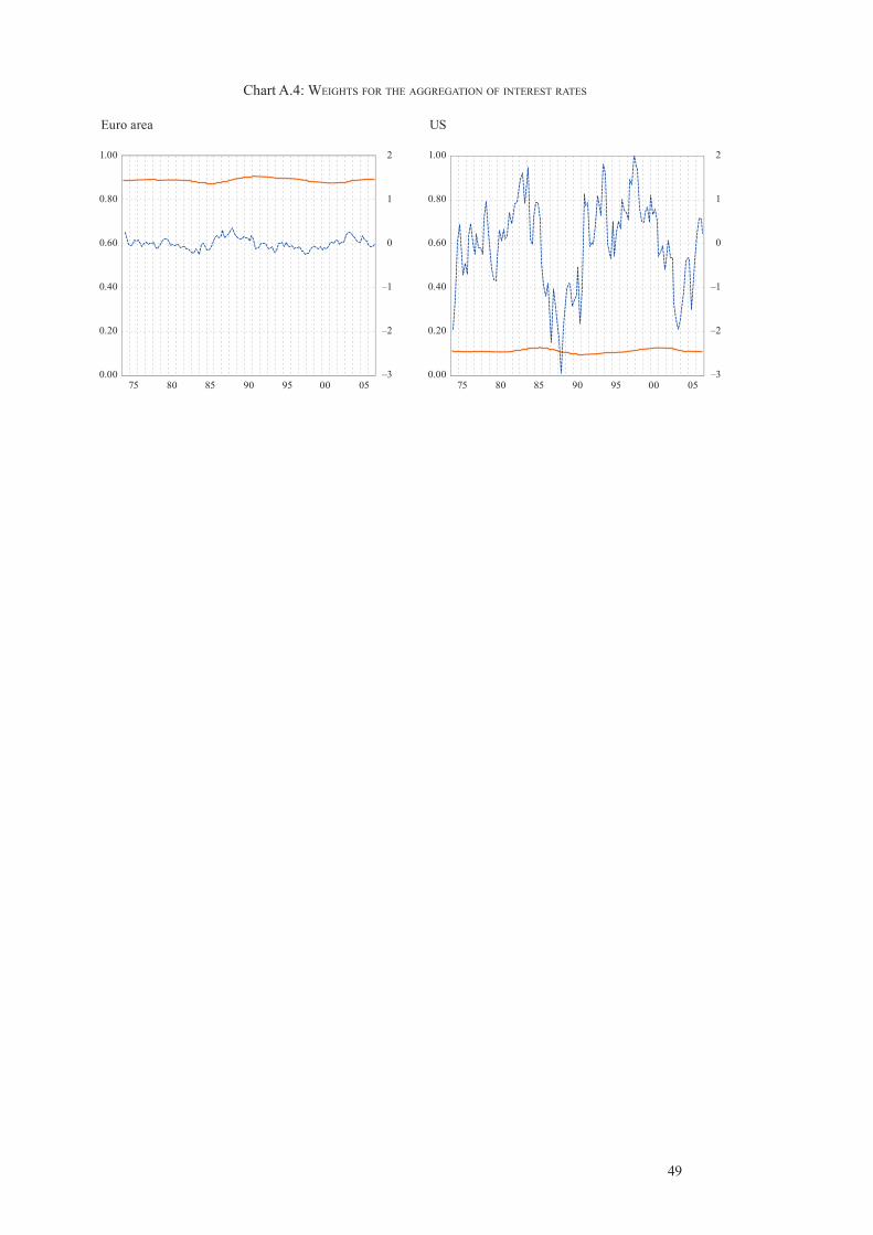
49

Chart A.4: WEIGHTS FOR THE AGGREGATION OF INTEREST RATES

75 80 85 90 95 00 05

1.00

0.80

0.60

0.40

0.20

0.00

2

1

0

–1

–2

–3 75 80 85 90 95 00 05

1.00

0.80

0.60

0.40

0.20

0.00

2

1

0

–1

–2

–3

Euro area US

50

References

Assenmacher-Wesche, Katrin and M. Hashem Pesaran. 2008. Forecasting the Swiss Economy Using VECX* Models: An Exercise in Forecast Combination across Models and Observation Windows. National Institute Economic Review No. 203, January: 91–108.

Dees, Stephane, Filippo di Mauro, M. Hashem Pesaran and L. Vanessa Smith. 2007. Exploring the International Linkages of the Euro Area: A Global VAR analysis. Journal of Applied Econometrics 22: 1–38.

Elliot, Graham, Thomas J. Rothenberg and James H. Stock. 1996. Effi cient Tests for an Autoregressive Unit Root. Econometrica 64: 813–836.

Garratt, Anthony, Kevin Lee, M. Hashem Pesaran and Yongcheol Shin. 2003. A Long Run Structural Macroeconometric Model of the UK. Economic Journal 113: 412–455.

Garratt, Anthony, Kevin Lee, M. Hashem Pesaran and Yongcheol Shin. 2006. Global and National Macroeconometric Modelling: A Long Run Structural Approach. Oxford University Press, Oxford.

Hansen, Henrik and Søren Johansen. 1999. Some Tests for Parameter Constancy in Cointegrated VAR-Models. Econometrics Journal 2: 306–333.

Ho, Mun S. and Bent E. Sørensen. 1996. Finding Cointegration Rank in High Dimen-sional Systems Using the Johansen Test: An Illustration Using Data Based Monte Carlo Simulations. Review of Economics and Statistics 78: 726–732.

Kilian, Lutz. 2002. Impulse Response Analysis in Vector Autoregressions with Unknown Lag Order. Journal of Forecasting 20: 161–179.

Kongsted, Hans Christian. 2005. Testing the Nominal-to-Real Transformation. Jour-nal of Econometrics 124: 205–225.

Koop, Gary, M. Hashem Pesaran and Simon Potter. 1996. Impulse Response Analysis in Nonlinear Multivariate Models. Journal of Econometrics 74: 119–147.

Lee, Kevin and M. Hashem Pesaran. 1993. Persistence Profi les and Business Cycle Fluctuations in a Disaggregated Model of UK Output Growth. Ricerche Econo-miche 47: 293–322.

Lütkepohl, Helmut. 2006. New Introduction to Multiple Time Series Analysis. 2nd ed. Springer, Berlin.

Nyblom, Jukka. 1989. Testing for the Constancy of Parameters Over Time. Journal of the American Statistical Association 84: 223–230.

Pagan, Adrian R. and M. Hashem Pesaran. 2008. Econometric Analysis of Structural Systems with Permanent and Transitory Shocks. Journal of Economic Dynamics and Control 32: 3376–3395.

Park, Heon Jin and Wayne A. Fuller. 1995. Alternative Estimators and Unit Root Tests for the Autoregressive Process. Journal of Time Series Analysis 16: 415–429.

Pesaran, M. Hashem and Yongcheol Shin. 1996. Cointegration and Speed of Conver-gence to Equilibrium. Journal of Econometrics 71: 117–143.

Pesaran, M. Hashem and Yongcheol Shin. 1999. An Autoregressive Distributed-Lag Modelling Approach to Cointegration. In Econometrics and Economic Theory in the 20th Century, S. Strom (ed.), 371–413. Cambridge University Press, Cambridge.

51

Pesaran, M. Hashem and Ron Smith. 2006. Macroeconometric Modelling with a Global Perspective. The Manchester School 74: 24–49.

Pesaran, M. Hashem, Til Schuermann, and Scott M. Weiner. 2004. Modelling Regional Interdependencies using a Global Error Correcting Macroeconometric Model. Journal of Business and Economic Statistics 22: 129–162.

Pesaran, M. Hashem, Yongcheol Shin and Richard J. Smith. 2000. Structural Analy-sis of Vector Error Correction Models with Exogenous I(1) Variables. Journal of Econometrics 97: 293–343.

Pesaran, M. Hashem, Yongcheol Shin and Richard J. Smith. 2001. Bounds Testing Approaches to the Analysis of Level Relationships. Journal of Applied Econo-metrics 16: 289–326.

Documents

Swiss National Bank Economic Studies · 2017-05-05 · Swiss National Bank Economic Studies No. 6 2009 A VECX* model of the Swiss economy* Katrin Assenmacher-Weschea and M. Hashem