Embed Size (px)
Citation preview
Switching Controllers: Realization,
Initialization and Stability
Jonathan PaxmanChurchill College
Control Group
Department of Engineering
University of Cambridge
A dissertation submitted for
the degree of Doctor of Philosophy
October 2003


For Ciaran

Preface
I would like to express my deep gratitude to my supervisor Dr Vinnicombe. His engineering
intuition and mathematical rigour have been an outstanding example to me. Our discussions
have always been interesting and fruitful.
I would also like to thank Keith Glover, Jan Maciejowski, Malcolm Smith, and John
Lygeros for their help, advice and academic leadership during my time in Cambridge.
There are many people (too many to name) whose friendship and support have made my
time in Cambridge more enjoyable. I owe my thanks to all of them.
Thanks also to all of my colleagues in the Control Group for friendship, technical advice,
intellectual challenges, animated discussions and beers on a Friday. It has been a privilege to
work in such an open and supportive environment.
Most especially I wish to thank my wife Rachael. Her love, support and patience has
been boundless.
Declaration: As required by University Statute, I hereby declare that this dissertation is my
own work and contains nothing which is the outcome of work done in collaboration with
others, except as specified in the text. I also declare that the length of this thesis is not more
than 60,000 words.
Jonathan Paxman
Cambridge, 2003
ii

Abstract
In the design of switching control systems, the choice of realizations of controller transfer
matrices and the choice of initial states for controllers (at switching times) are of critical
importance, both to the stability and performance of the system.
Substantial improvements in performance can be obtained by implementing controllers
with appropriate realizations. We consider observer form realizations which arise from
weighted optimizations of signals prior to a switch. We also consider realizations which
guarantee stability for arbitrary switches between stabilizing controllers for a linear plant.
The initial value problem is of crucial importance in switching systems, since initial state
transients are introduced at each controller transition. A method is developed for determining
controller states at transitions which are optimal with respect to weighted closed-loop per-
formance. We develop a general Lyapunov theory for analyzing stability of reset switching
systems (that is, those switching systems where the states may change discontinuously at
switching times). The theory is then applied to the problem of synthesizing controller reset
relations such that stability is guaranteed under arbitrary switching. The problem is solved
via a set of linear matrix inequalities.
Methods for choosing controller realizations and initial states are combined in order to
guarantee stability and further improve performance of switching systems.
Keywords: bumpless transfer, antiwindup, coprime factorization, switching control, con-
troller conditioning, stability.
iii

Contents
Preface ii
Abstract iii
Table of Contents iv
Notation and Abbreviations ix
1 Introduction 1
1.1 Bumpless transfer and conditioning . . . . . . . . . . . . . . . . . . . . . . . . 3
1.2 Controller initialization in a switching architecture. . . . . . . . . . . . . . . . 4
1.3 Overview . . . . . . . . . . . . . . . . . . . . . . . . . . . . . . . . . . . . . 5
2 Preliminaries 9
2.1 Spaces and functions .. . . . . . . . . . . . . . . . . . . . . . . . . . . . . . 9
2.2 Dynamical systems . . . . . . . . . . . . . . . . . . . . . . . . . . . . . . . . 12
2.3 Hybrid dynamical systems . . . . .. . . . . . . . . . . . . . . . . . . . . . . 14
2.4 Stability . . . . . . . . . . . . . . . . . . . . . . . . . . . . . . . . . . . . . . 15
2.4.1 Stability of hybrid systems . .. . . . . . . . . . . . . . . . . . . . . . . 18
2.5 Lyapunov functions for stability analysis . . . . .. . . . . . . . . . . . . . . . 19
2.5.1 Converse theorems . . . . . . . . . . . . . . . . . . . . . . . . . . . . . 20
2.5.2 Non-smooth Lyapunov functions . . . . . .. . . . . . . . . . . . . . . . 22
2.6 Bumpless transfer and connections to the anti-windup problem . . . .. . . . . 23
2.6.1 Conventional antiwindup . . .. . . . . . . . . . . . . . . . . . . . . . . 24
2.6.2 Hanus conditioned controller . . . . . . . . . . . . . . . . . . . . . . . . 26
v

vi CONTENTS
2.6.3 Internal Model Control . . . . . . . . . . . . . . . . . . . . . . . . . . . 27
2.6.4 Observer based schemes . . . . . . . . . . . . . . . . . . . . . . . . . . 27
2.6.5 Unifying standard techniques . . . . . . . . . . . . . . . . . . . . . . . . 29
2.6.6 Coprime factorization approach . . . . . . . . . . . . . . . . . . . . . . 30
2.7 Filtering and estimation . .. . . . . . . . . . . . . . . . . . . . . . . . . . . . 32
2.7.1 Discrete-time equations . . . . . . . . . . . . . . . . . . . . . . . . . . . 33
2.7.2 Continuous-time equations .. . . . . . . . . . . . . . . . . . . . . . . . 35
2.8 The deterministic filtering problem . . . . . . . . . . . . . . . . . . . . . . . . 35
2.8.1 Continuous-time equations .. . . . . . . . . . . . . . . . . . . . . . . . 36
2.8.2 Discrete-time equations . . . . . . . . . . . . . . . . . . . . . . . . . . . 36
3 Stability of simple switching systems 39
3.1 Common Lyapunov functions for switching systems . . . . .. . . . . . . . . . 42
3.2 Multiple Lyapunov functions . . .. . . . . . . . . . . . . . . . . . . . . . . . 44
3.3 Dwell time switching . . . . . . . . . . . . . . . . . . . . . . . . . . . . . . . 46
3.3.1 Dwell times for linear simple switching systems . . . . . . . . . . . . . . 47
3.4 Choice of controller realizations . . . . . . . . . . . . . . . . . . . . . . . . . 52
3.4.1 IMC approach . . . . . . . . . . . . . . . . . . . . . . . . . . . . . . . 52
3.4.2 Choice of coprime factorizations . . . . . . . . . . . . . . . . . . . . . . 53
3.5 Concluding remarks . . . . . . . . . . . . . . . . . . . . . . . . . . . . . . . . 56
4 Controller conditioning for switching 57
4.1 Controller state selection via a noise minimization problem . . . . . . . . . . . 57
4.2 Discrete-time explicit solution . . . . . . . . . . . . . . . . . . . . . . . . . . 58
4.2.1 Scheme applied to basic example . . . . . . . . . . . . . . . . . . . . . 61
4.3 Kalman filter implementation . . . . . . . . . . . . . . . . . . . . . . . . . . . 62
4.4 Implementation issues . . . . . . . . . . . . . . . . . . . . . . . . . . . . . . . 63
4.5 Time invariant equations . . . . . . . . . . . . . . . . . . . . . . . . . . . . . 63
4.6 Coprime factor representation . . . . . . . . . . . . . . . . . . . . . . . . . . . 65
4.6.1 Special case weighting . . . . . . . . . . . . . . . . . . . . . . . . . . . 66
4.6.2 The reference problem . . . . . . . . . . . . . . . . . . . . . . . . . . . 67
4.7 Concluding remarks . . . . . . . . . . . . . . . . . . . . . . . . . . . . . . . . 69

CONTENTS vii
5 Controller initialization: optimal transfer 71
5.1 Discrete time . . . . . . . . . . . . . . . . . . . . . . . . . . . . . . . . . . . 71
5.1.1 Finite horizon solution . . . . . . . . . . . . . . . . . . . . . . . . . . . 73
5.1.2 Infinite horizon solution . . . . . . . . . . . . . . . . . . . . . . . . . . 74
5.1.3 Lyapunov function interpretation . . . . . .. . . . . . . . . . . . . . . . 75
5.1.4 Weighted solution . . . . . . . . . . . . . . . . . . . . . . . . . . . . . . 76
5.2 Continuous time . . . .. . . . . . . . . . . . . . . . . . . . . . . . . . . . . . 77
5.3 Plant state estimation . . . . . . . . . . . . . . . . . . . . . . . . . . . . . . . 81
5.4 Problems with non-zero reference .. . . . . . . . . . . . . . . . . . . . . . . 82
5.5 Examples . . . . . . . . . . . . . . . . . . . . . . . . . . . . . . . . . . . . . 84
5.5.1 Initialization scheme applied to example 1 .. . . . . . . . . . . . . . . . 84
5.6 Concluding remarks . . . . . . . . . . . . . . . . . . . . . . . . . . . . . . . . 84
6 Stability of reset switching systems 87
6.1 A Lyapunov theorem for reset switching systems. . . . . . . . . . . . . . . . 88
6.2 Controller initialization . . . . . . . . . . . . . . . . . . . . . . . . . . . . . . 93
6.2.1 Quadratic Lyapunov functions. . . . . . . . . . . . . . . . . . . . . . . 99
6.3 Reset synthesis for stability . . . . .. . . . . . . . . . . . . . . . . . . . . . . 101
6.4 Reset switching of coprime factor controllers . . . . . . . . . . . . . . . . . . 106
6.5 Plant state estimation . . . . . . . . . . . . . . . . . . . . . . . . . . . . . . . 109
6.6 Multiple Lyapunov functions for reset systems . .. . . . . . . . . . . . . . . . 116
6.7 Dwell times and reset switching systems . . . . . . . . . . . . . . . . . . . . . 118
6.8 Concluding remarks . . . . . . . . . . . . . . . . . . . . . . . . . . . . . . . . 120
7 Conclusions 123
7.1 Summary of main contributions . . . . . . . . . . . . . . . . . . . . . . . . . . 124
7.2 Opportunities for further investigation . . . . . .. . . . . . . . . . . . . . . . 125
7.2.1 General . . . . . . . . . . . . . . . . . . . . . . . . . . . . . . . . . . . 126

viii CONTENTS
A Some basic results 127
A.1 Matrix inversion lemma . . . . . . . . . . . . . . . . . . . . . . . . . . . . . . 127
A.2 Least squares optimisation . . . . . . . . . . . . . . . . . . . . . . . . . . . . 127
A.3 Closed loop equations . . . . . . . . . . . . . . . . . . . . . . . . . . . . . . . 129
A.3.1 Continuous-time . .. . . . . . . . . . . . . . . . . . . . . . . . . . . . 129
A.3.2 Discrete-time . . . . . . . . . . . . . . . . . . . . . . . . . . . . . . . . 130
A.4 Continuous-time Lyapunov equation . . . . . .. . . . . . . . . . . . . . . . . 131
Bibliography 133

Notation and Abbreviations
Notation
R field of real numbers
R+ field of non-negative real numbers
Z field of integers
Z+ field of non-negative integers
C field of complex numbers
H∞ Hardy∞ space
∈ belongs to
∀ for all
∃ there exists
:= defined to be equal to
2 end of proof
‖x‖ the norm of vectorx, assumed to be the
Euclidean norm where no other is specified
A∗ the conjugate transpose of matrixA,
or whereA is real valued, the transpose
A† left matrix pseudo inverse ofA, A† = (A∗A)−1A∗
mint(x) minimum ofx with respect tot
argmint
(x) the value oft which minimisesx
=⇒ implies
⇐⇒ if and only if
x the derivative ofx with respect to timedxdt
f : X→ Y A function f mapping a setX into a setY
ix

x NOTATION AND ABBREVIATIONS
Abbreviations
LTI linear time invariant
LMI linear matrix inequality
SISO single input single output
AWBT antiwindup bumpless transfer
IMC internal model control
CAW conventional antiwindup
CLF Common Lyapunov Function
QLF Quadratic Lyapunov Function
CQLF Common Quadratic Lyapunov Function

Chapter 1
Introduction
Switching control is one way of dealing with design problems in which the control objectives,
or system models are subject to change. It is common, for example to design linear controllers
for a number of different linearized operating points of a nonlinear plant, and then seek to
switch between the controllers in a sensible way. Switching control may also be appropriate
when the plant is subject to sudden changes in dynamic behaviour (for example gear changes
in some engine and motor control problems).
A general switching architecture is illustrated in figure 1.1. The (linear or nonlinear)
process to be controlled isP, for which N controllers have been designed. A high level
controller or switching supervisorSgoverns the switching process, based on measurements
of the plant input and output, and an external command signalh, which may or may not be
related to the referencer . Theresetmechanism allows for the possibility that the controllers
may be reinitialized in some way at each switching transition.
hreset
u y
r
P
K1
K2
KN
S
Figure 1.1: General switching architecture
1

2 Introduction
A switching architecture has certain advantages over other multi-controller approaches
such as gain scheduling. A family of controllers employed for gain scheduling must have the
same order and structure, whereas a switching family require only that the input and output
dimensions are consistent. There can also be benefits arising from the transients introduced
by a hard switch. In observer switching architectures, information is provided about the plant
mode which allows the correct controller to be applied with greater certainty.
Transient signals caused by hard switching can also be a burden on performance. If the
controller realization and initialization strategy are poorly designed for switching, substantial
transient signals caused by the switching can degrade performance and lead to instability.
The choice of controller realization is a much more important matter for switching systems
than for other control problems. In a single (non-switching) ideal control loop, the realization
of the controller ceases to be relevant once initial state transients have died down. In a
switching architecture however, the realization has an effect every time a switch takes place.
The realization is also important when other nonlinearities such as saturation are present.
For similar reasons, the initialization of controllers is important when considering a switch-
ing architecture. Should switching controllers (if same order) share state space? Should they
retain previous values? Or should they be reinitialized to zero or some other value at each
switch? These questions are vitally important to the performance of a switching system.
Stability of switching systems is not a simple matter, even when everything is linear and
ideal. It is possible to switch between two stabilizing controllers for a single linear plant in
such a way that an unstable trajectory results. In such circumstances, it is possible to ensure
stability by choice of appropriate controller realizations, or by sensible choices of controller
initializations (or both).
This dissertation is primarily concerned with realizing and initializing controllers for
switching systems in ways which ensure stability and enhance performance.
In general we will consider the idealized scenario of a single linear plant and a family of
stabilizing linear controllers. The switching signal will usually be assumed to be unknown.
We focus on the choice of realization of the controllers and the initialization (or reset) strategy
for the controllers. Our methods are generally independent of the controller design and
switching strategy design, and therefore fit very well in a four step design process.
i. Controller design
ii. Controller realization
iii. Reset strategy design
iv. Switching strategy design

1.1 Bumpless transfer and conditioning 3
Controller transfer matrices are designed using conventional linear methods and then the
realizations and reset strategies are determined in order to guarantee stability and minimize
performance degradation due to the switching process. Switching strategy design is the last
step, allowing for the possibility of real-time or manual switching. The switching strategy
may be implemented via a switching supervisor or high level controller as illustrated in
figure 1.1. The switching strategy in some applications may be determined manually. We
examine briefly the problem of switching strategy, considering the calculation of minimum
dwell times for switching systems to ensure stability given fixed controller realizations (with
or without resets).
1.1 Bumpless transfer and conditioning
The so-calledbumpless transferproblem has received considerable attention in the literature.
The term usually refers to situations where we wish to carry out smooth (in some sense)
transitions between controllers. The precise definition of a bumpless transfer is not universally
agreed.
Some authors (see [1,29] for example) refer to a bumpless transfer as one where continuous
inputs result in continuous outputs regardless of controller transitions. This definition is
not often very useful, since controller transitions can cause very large transient signals in
the outputs, even when the signals remain continuous (for example if the plant has a high
frequency roll off). The definition is also unhelpful if the system is discrete-time.
Other authors (see [13,55,56] for example) refer to bumpless transfer when the difference
between signals produced by (and driving) the on-line and off-line controllers are minimal in
some sense. Our methods introduced in chapter 4 are based on similar definitions of bumpless
transfer.
The third approach is to consider that bumpless transfer occurs if the transients introduced
by the controller transitions are minimal in some sense. This definition, or one similar to it has
been considered by Graebe and Ahlèn [18] and also by Peng, Hanus and coauthors [49,23].
The latter authors sometimes use the termconditioned transferto distinguish between this
property and one where continuity is the aim. Our methods in chapter 5 and subsequent
stabilization methods in chapter 6 are connected with this idea.
Example 1.1.1.Consider the following plant transfer function
P = 1
s(s2+ 0.2s+ 1). (1.1)

4 Introduction
u2
u1
u yr PK
Figure 1.2: Generalized input substitution
The controller is a suboptimal robust controller. The designed continuous controller is
K =
0.8614 −0.1454 −0.0798
0.1183 0.9705 −0.4647
0.0042 0.0641 0.6094
−0.0081
0.3830
0.3260
[−1.4787 −0.9166 −1.1978
][0]
. (1.2)
We consider here the regulator problem. That is, we have reference inputr = 0.
We use the above plant and controller, discretized with a sampling timeT = 0.05. We
drive the plant open loop by a random noise signal (sampled with period 10)u1 and switch to
the outputu2 of controllerK at timek = 160. The system is set up as illustrated in figure 1.2.
No conditioning is applied to the controller prior to the switch, so the controller state remains
zero until the switching instant. Figure 1.3 shows the plant input and output for the system
as described.
We can clearly observe a substantial transient which follows the switch (particularly in the
plant input).
One measure of the “size” of the transient, is thel2[n,∞) norm of the signal[
u
y
], where
n is the switching time. In this example the norm is 17.46. We will return to this example
later, showing the results of some conditioning and initialization schemes.
1.2 Controller initialization in a switching architecture
The controller initial value problem is often not an important consideration in conventional
control frameworks. When a single controller is used, the effect of the initial state of the
controller is typically limited to the initial transients of the system. Provided that the controller
is sensibly designed, a zero initial state is usually quite acceptable. Furthermore, optimal

1.3 Overview 5
0 50 100 150 200 250 300 350 400 450 500−3
−2
−1
0
1
2
time
plan
t inp
ut
0 50 100 150 200 250 300 350 400 450 500−1
0
1
2
3
4
time
plan
t out
put
Figure 1.3: Unconditioned response to switch at k=160
initialization of controllers may be impossible if the initial state of the plant is not known. In
an output feedback scenario, it may be necessary to run the controller for some time before
an observer is able to capture the plant state with a reasonable error margin.
In a switching architecture however, the initial value problems can be extremely important.
If new controllers are periodically introduced into the feedback loop, then transients signals
due to the initial states of the controllers will occur at each transition. These transient signals
can substantially degrade the performance of the resulting systems. If the plant dynamics are
assumed to be remain the same, (or at least slowly time-varying) then we may have a great deal
of information about the plant states when we switch to a new controller. This information
may then be exploited in the solution of the initial value problem at each transition.
1.3 Overview
Chapter 2
Some preliminary material required in the rest of the thesis is introduced. We define some
mathematical terminology and notation, particularly associated with dynamical systems and
hybrid systems in particular.
We review Lyapunov stability theory and in particular some results concerning the exis-
tence of Lyapunov functions and also admissibility of non-smooth Lyapunov functions.

6 Introduction
The notionreset switching systemis introduced, referring to a switching system where
the states may change discontinuously at switching boundaries. We also use the termsimple
switching systemto refer to switching systems where the states remain continuous across
switching boundaries.
We present a brief summary of approaches to the bumpless transfer problem in the lit-
erature, including some unified frameworks, and review connections with the anti-windup
problem.
We briefly describe the general state estimation problem and present the continuous and
discrete-time Kalman filter equations. We also note that the Kalman filter equations can be
derived in a purely deterministic context, following the work of Bertsekas and Rhodes [5].
Chapter 3
A review of results concerning the stability of simple switching systems is presented. We
introduce results concerning stability (under arbitrary switching) guaranteed by the existence
of a common Lyapunov function for the component systems(by Barmish [4] and others), and
in particular the converse result by Dayawansa and Martin [10].
We study the Multiple Lyapunov function approach to the study of stability of switching
systems introduced by Branicky [7].
We introduce the notion of minimum dwell-time as a means for ensuring stability of
switching systems as introduced by Morse [46]. Some tighter dwell-time results are presented
based on quadratic Lyapunov functions.
Two results are presented which guarantee the existence of realizations of stabilizing
controllers such that the switching system is guaranteed to be stable under arbitrary switching.
Chapter 4
We introduce a bumpless transfer approach which is based on calculation of controller states
at transitions which are compatible with input-output pairs in the graph of the controller (to
be switched on) and close in some sense to the observed signals.
The solution is presented initially as a weighted least squares optimization. We note that
the solution can be implemented as a on observer controller with an optimal Kalman observer
gain. Thus the solution can be implemented by an appropriate choice of controller realization
without requiring resets to the controller states.

1.3 Overview 7
Chapter 5
We introduce an alternative approach to the bumpless transfer problem which is based on
choosing controller states which minimize explicitly the transients at each controller tran-
sition. The finite horizon problem is solved via a least squares minimization. The infinite
horizon solution is solved via Lyapunov equations. The infinite horizon solution is thus also
equivalent to minimization of Lyapunov functions with respect to the controller states. A
weighted solution can be employed to account for known average dwell times.
Chapter 6
We study the stability of reset switching systems. We introduce a necessary and sufficient
Lyapunov theorem for reset switching systems to be stable under arbitrary switching. We
study a number of important consequences of this result, including conditions which guarantee
stability for linear reset switching systems under arbitrary switching.
Sufficient LMI conditions allow for the synthesis of reset relations which guarantee sta-
bility. While such stabilizing resets do not always exist for given controller realizations, we
show that these results can be combined with known stabilizing realizations with guaranteed
stability, and a substantial improvement in performance.
Chapter 7
We summarize the conclusions of the thesis, and review the original contributions.


Chapter 2
Preliminaries
This chapter introduces some of the basic mathematical terms and definitions which are used
in this thesis, along with some fundamental results which are required for proofs in later
chapters. Where proofs are omitted, textbook references are provided.
2.1 Spaces and functions
Definitions and results relating to this section may be found in any elementary analysis text
such as [38,6,51].
Definition 2.1.1. A metric spaceis a pair(X, d), whereX is a set andd is a function from
X × X toR+ satisfying
• d(x, y) = 0 ⇐⇒ x = y
• d(x, y) = d(y, x) for all x, y ∈ X
• d(x, z) ≤ d(x, y)+ d(y, z) for all x, y, z ∈ X
d(x, y) is referred to as thedistancebetweenx andy. d is referred to as themetricon X.
The third condition above is thetriangle inequality.
Definition 2.1.2. A normed spaceis a pair(X, ‖.‖), whereX is a vector space overR orC,
and‖.‖ is a function fromX toR+ satisfying
• ‖x‖ = 0 ⇐⇒ x = 0
• ‖λx‖ = |λ| ‖x‖ for all x ∈ X, andλ ∈ R
9

10 Preliminaries
• ‖x + y‖ ≤ ‖x‖ + ‖y‖ for all x, y ∈ X
‖x‖ is referred to as thenormof vectorx, and may be thought of as the ’length’ of the vector
in a generalized sense. The third condition above is thetriangle inequality.
Every normed space is also a metric space with the induced metricd(x, y) = ‖x − y‖.Definition 2.1.3. A sequence{xn} in a metric spaceX is Cauchyif for all ε ∈ R+, there
existsN ∈ Z+ such that min{i, j } > N impliesd(xi , xj ) < ε.
Definition 2.1.4. A metric spaceX is completeif every Cauchy sequence inX converges to
an element ofX. A complete normed space is also called aBanachspace.
A complete space is essentially one which has no ’holes’ in it.
In a normed spaceX, thesphereof radiusr about a pointx0 is
Sr (x0) = {x ∈ X : ‖x − x0‖ = r }.
The (closed)ball of radiusr about a pointx0 is
Br (x0) = {x ∈ X : ‖x − x0‖ ≤ r }.
Theopen ballof radiusr about a pointx0 is
Dr (x0) = {x ∈ X : ‖x − x0‖ < r }.
An open ball about a pointx0 is sometimes called aneighbourhoodof x0.
Definition 2.1.5. A function between metric spacesf : X → Y is calledcontinuousat a
point x, if f (xk) → f (x) wheneverxk → x. Equivalently, f is continuous if for every
ε > 0, there existsδ > 0 such that
d(x, y) < δ =⇒ d( f (x), f (y)) < ε.
f is continuous onX if it is continuous at every point inX. If δ of the inequality depends
only onε, and not onx, then the function isuniformly continuous.
Definition 2.1.6. A function between metric spacesf : X → Y satisfies theLipschitz
conditionon a domain� if there exists a constantk ≥ 0 such that
d( f (x), f (y)) ≤ kd(x, y) ∀x, y ∈ �.
f is globally Lipschitzif the condition is satisfied for the whole ofX.

2.1 Spaces and functions 11
This property is sometimes referred to asLipschitz continuity, and it is in fact a stronger
condition than uniform continuity.
The following definitions concern scalar functions of a Banach spaceV : X → R or on
a Banach space and timeW : X × R+ → R (W : X × Z+ → R in the discrete-time case).
Let� be a closed bounded region inX, andx be an element ofX.
Definition 2.1.7. A scalar functionV(x) is positive semi-definite(resp. negative semi-
definite) in � if, for all x ∈ �,
• V(x) has continuous partial derivatives with respect tox
• V(0) = 0
• V(x) ≥ 0 (resp.V(x) ≤ 0)
Definition 2.1.8. A scalar functionV(x) is positive definite(resp.negative definite)in � if,
for all x ∈ �,
• V(x) has continuous partial derivatives with respect tox
• V(0) = 0
• V(x) > 0 (resp.V(x) < 0) if x 6= 0
Definition 2.1.9. A (time dependent) scalar functionW(x, t) is positive semi-definite(resp.
negative semi-definite) in � if, for all x ∈ � and allt ,
• W(x, t) has continuous partial derivatives with respect to it’s arguments
• W(0, t) = 0 for all t
• W(x, t) ≥ 0 (resp.W(x, t) ≤ 0) for all t
Definition 2.1.10.A (time dependent) scalar functionW(x, t) is positive definite(resp.neg-
ative definite) in � if, for all x ∈ � and allt ,
• W(x, t) has continuous partial derivatives with respect to it’s arguments
• W(0, t) = 0 for all t
• W(x, t) > 0 (resp.W(x, t) < 0) for all t
Definition 2.1.11. A scalar functionW(x, t) is decrescentin � if there exists a positive
definite functionV(x) such that for allx ∈ �, and allt
W(x, t) ≤ V(x).

12 Preliminaries
This property is also referred to as “W admits an infinitely small upper bound”, or “W
becomes uniformly small”. It is equivalent to saying thatW can be made arbitrarily small by
choosingx sufficiently close to 0. Any time-invariant positive definite function is decrescent.
Definition 2.1.12. A scalar functionV(x) is radially unboundedin � if V(x) → ∞ as
‖x‖ → ∞.
Definition 2.1.13. A (time dependent) scalar functionW(x, t) is radially unboundedin� if
there exists a positive definite radially unbounded functionV(x) such that
W(x, t) ≥ V(x) ∀t .
That is,W(x, t) tends to infinity uniformly int as‖x‖ → ∞.
2.2 Dynamical systems
Broadly speaking, a dynamical system involves the motion of some objects through a space as
a function of time. We use the notionstateto represent some parameter or set of parameters
which completely capture the position and behaviour of a system at any one point in time.
To describe a dynamical system completely, we must define carefully thephase space, or
state spaceof the system - or the set of admissible values for the state. The phase space of a
dynamical system is typically a Banach space. We must define thetime spaceof the system,
which is typicallyR+ (continuous-time) orZ+ (discrete-time). We then must have some way
of describing the evolution of the system from one point in time to the next. In the systems we
consider, the evolution of the state is usually described by families of differential equations
(continuous-time case) or difference equations (discrete-time case). When we consider hybrid
or switching systems, we also usereset relationsin describing state evolution. We may also
introduce aninput which externally influences the behaviour of the system, the input being
taken from a specifiedinput space.
Consider systems described by continuous first-order ordinary differential equations
x(t) = f (x(t), t, u(t)) x(t) ∈ X, t ∈ R+, u(t) ∈ U, (2.1)
or by continuous first-order difference equations
x(k+ 1) = f (x(k), k, u(k)) x(k) ∈ X, k ∈ Z+, u(k) ∈ U. (2.2)
X is the phase space of the system, andU the input space.

2.2 Dynamical systems 13
We may also define an outputy(t) ∈ Y (respy(k) ∈ Y) with theoutput spaceY a Banach
space, andy defined by the equations
y(t) = f (x(t), t, u(t)) x(t) ∈ X, t ∈ R+, u(t) ∈ U, (2.3)
or
y(k) = f (x(k), k, u(k)) x(k) ∈ X, k ∈ Z+, u(k) ∈ U. (2.4)
In the systems we consider, the phase (and input and output) spaces are continuous (X =Rn), or discrete (X = Zn), or some combination (X = Rn × Zm). The time space isR+ in
the continuous-time case, orZ+ in the discrete-time case.
In the following sections, we will occasionally omit the discrete-time version of a result or
definition, where the discrete-time counterpart is completely analogous to the continuous-time
version.
If u(t) = 0 for all t , a system is referred to asunforced, or free, and may be represented
by the unforced equations
x(t) = f (x(t), t) x(t) ∈ X, t ∈ R+, (2.5)
or
x(k+ 1) = f (x(k), k) x(k) ∈ X, k ∈ Z+. (2.6)
Note that a system with a fixed known inputu(t) can also be thought of as a free system
described by the equations above, withu(t) being implicit in the functionf (x(t), t). Where
u(t) is explicit we refer to aforcedsystem.
The solution of an unforced system with given initial conditionsx0 andt0 is known as the
trajectoryof the system, and may be denoted byφ(t, x0, t0).
Existence and uniqueness of trajectories defined in this way can be guaranteed by ensuring
that the right hand side of the differential (resp difference) equation satisfies a Lipschitz
condition (see for example [28])
‖ f (x, t), f (y, t)‖ ≤ k ‖x − y‖ .
We shall assume this condition for all vector fields considered in this thesis.
A dynamical system so described is called stationary if the functionsf above do not depend
explicitly on t (respk). An unforced stationary system is sometimes calledautonomous, and
may be described by time invariant equations
x(t) = f (x(t)), (2.7)
or
x(k+ 1) = f (x(k)). (2.8)

14 Preliminaries
2.3 Hybrid dynamical systems
The word ‘Hybrid’ has come to characterize classes of dynamical systems which combine
continuous and discrete dynamics. In particular, the state of a hybrid system usually has both
discrete and continuous components. TypicallyX = Rn×Z (noting thatZm is equivalent to
Z).
We introduce some classes of Hybrid systems which include the switching controller
systems that we consider in later chapters.
The evolution of the ‘continuous-valued’ states of the system are governed by ordinary
differential equations (or difference equations), while the discrete state is governed by some
discrete valued function.
Consider the family of systems
x(t) = fi (x(t)), i ∈ I , x(t) ∈ Rn. (2.9)
whereI is some index set (typically discrete valued).
Now define a piecewise constantswitching signalσ(t)
σ (t) = i k tk ≤ t < tk+1, i k ∈ I (2.10)
for some sequence of times{tk} and indices{i k} (k ∈ Z+). We assume thattk < tk+1 and
i k 6= i k+1 for all k. We will call {tk} theswitching timesof the system. We may also use the
termswitching trajectoryfor σ .
σ(t) is known as anon-zenosignal, if there are finitely many transitions in any finite time
interval. Signals need to be non-zeno in order that trajectories are well defined for all time.
Furthermore, we shall callσ(t) strongly non-zenoif the ratio of the number of transitions in
a finite time interval to the length of the time interval has a fixed upper bound. In general
sensible switching strategies will result in strongly non-zeno switching signals. We will
usually assume switching signals to be strongly non-zeno.
Now we may describe the followingsimple switching system
x(t) = fσ(t)(x(t)),
σ (t) = i k, ∀ tk ≤ t < tk+1, i k ∈ I , k ∈ Z+. (2.11)
That is, the evolution of the continuous state of the system is described by the vector fieldfikin the interval[tk, tk+1). Thediscrete stateof the system may be thought of as the value of
the functionσ(t) at any given timet .
A simple switching system with a fixed switching signalσ(t) may be thought of simply
as a time varying continuous system described by a single time-varying vector field (such as
2.5). For a more general problem, we examine classes of admissible switching signals.

2.4 Stability 15
Another class of hybrid systems allows the statex to change discontinuously at switching
times. This allows us to describe for example physical systems with instantaneous collisions
(see for example [57]). In our case, we use this description for plant/controller systems with
switching controllers, where the controller state may be reset in some manner at each switch
(such as to minimize transients of a weighted output of the closed loop system).
Let us introduce a family of functions
gi, j : Rn→ Rn, i, j ∈ I .
The functionsgi, j describe the discontinuous change in state at the transition timestk.
Then areset switching systemmay be described by the equations
x(t) = fσ(t)(x(t)),
σ (t) = i k, ∀ tk ≤ t < tk+1, i k ∈ I , k ∈ Z+,x(t+k ) = gik,i k−1(x(t
−k )).
(2.12)
We call the functionsgi, j reset relationsbetween the discrete statesi and j . If gj ,i1 = gj ,i2
for eachi1, i2 ∈ I (that is, the reset only depends on the new state), then we may use the
shorthand notationgj .
We may also consider hybrid systems where the state space is not necessarily the same in
each discrete state. For example in switching controller systems, it is possible that alternative
controllers for the system are different order, or that linear models of the behaviour of a
nonlinear plant are different order at various set points. In this case, we consider the family
of systems
xi (t) = fi (xi (t)), i ∈ I , xi (t) ∈ Rni , (2.13)
and themultiple state-space switching systemmay be described as follows
xσ(t)(t) = fσ(t)(xσ(t)(t)), (2.14)
σ(t) = i k tk ≤ t < tk + 1, i k ∈ I , k ∈ Z+, (2.15)
xik(t+k ) = gik,i k−1(xik−1(t
−k )). (2.16)
Note that in this case, the reset relationsgi, j are required, since the state cannot be continuous
across switches when the state order changes.
2.4 Stability
An equilibrium stateof an unforced dynamical system, is a statexe such thatf (xe, t) = 0
for all t . Thus if the initial state of the system isxe, the trajectory of the system will remain at

16 Preliminaries
xe for all time. A trajectoryφ(t, xe, t0) is sometimes referred to as anequilibrium trajectory,
or equilibrium solution.
There are a large number of definitions available for the stability of a system. For unforced
systems, definitions generally refer to the stability of equilibria - specifically to the behaviour
of trajectories which start close to the equilibrium (sometimes calledperturbed trajectories).
For forced systems, stability usually refers to the relationship between output input functions.
We refer here to a few of the most useful stability definitions for unforced systems, begin-
ning with those discussed by Aleksandr Mihailovich Lyapunov in his championing work on
stability theory first published in 1892 [33].
A number of texts provide good references for this material, including [60,21,28].
Consider the dynamical system
x(t) = f (x(t), t) x(t) ∈ X, t ∈ R+,
with equilibrium statexe so that f (xe, t) = 0 for all t .
Definition 2.4.1. The equilibrium statexe is calledstableif for any givent0 andε > 0 there
existsδ > 0 such that
‖x0− xe‖ < δ =⇒ ‖φ(t, x0, t0)− xe‖ < ε
for all t > t0.
This property is also sometimes referred to as stable in the sense of Lyapunov. It essentially
means that perturbed trajectories always remain bounded.
Definition 2.4.2. The equilibrium statexe is calledconvergent, if for any t0 there existsδ1 > 0
such that
‖x0− xe‖ < δ1 =⇒ limt→∞φ(t, x0, t0) = xe.
That is, for anyε1 > 0 there exists aT > t0 such that
‖x0− xe‖ < δ1 =⇒ ‖φ(t, x0, t0)− xe‖ < ε1
for all t > T .
We say that the perturbed trajectoriesconvergeto the equilibrium state. Note that conver-
gence does not imply stability nor vice-versa.
Definition 2.4.3. The equilibrium statexe is calledasymptotically stableif it is both stable
and convergent.

2.4 Stability 17
If this property holds for allx0 ∈ X (not just in a neighbourhood ofxe), we say that
the state isglobally asymptotically stable. We can also then say that the system is globally
asymptotically stable.
Definition 2.4.4. A dynamical system is calledbounded, or Lagrange stableif, for any x0,
t0 there exists a boundB such that
‖φ(t, x0, t0)‖ < B
In definition 2.4.1,δ may generally depend ont0 as well asε.
Definition 2.4.5. If the equilibrium statexe is stable, and theδ (of definition 2.4.1) depends
only onε, then we can say that the equilibriumxe is uniformly stable.
Definition 2.4.6. If an equilibrium state is convergent, and theδ1 andT of definition 2.4.2
are independent oft0, then the state is known asuniformly convergent.
Definition 2.4.7. If an equilibrium state is bounded, and theB of definition 2.4.4 are inde-
pendent oft0, then the state is known asuniformly bounded.
Uniform boundedness and uniform stability are equivalent for linear systems.
Definition 2.4.8. If an equilibrium state is uniformly stable and uniformly convergent, then
it is uniformly asymptotically stable.
Definition 2.4.9. If an equilibrium state is uniformly stable, uniformly bounded, and globally
uniformly convergent, then it isglobally uniformly asymptotically stable.
We also say that the system itself is globally uniformly asymptotically stable. Note that
uniform stability and uniform convergence are not sufficient to guarantee uniform bounded-
ness (see for example [60]).
Definition 2.4.10. An equilibrium statexe is calledexponentially stableif the norm of tra-
jectories may be bounded above by a exponential function with negative exponent. That is,
for all t0, x0 there exist scalarsa > 0, b > 0 such that
‖φ(t, x0, t0)− xe‖ < a ‖x0− xe‖e−b(t−t0)
for all t > t0.
Definition 2.4.11. If, in addition the scalarsa andb may be found independently oft0 and
x0, then the state is calleduniformly exponentially stable.

18 Preliminaries
Exponential stability implies asymptotic stability, but not vice-versa. For instance the
function
x(t) = x0
t + 1
converges asymptotically to the origin, but is not bounded above by a decaying exponen-
tial function. For linear systems however, exponential stability is equivalent to asymptotic
stability [60].
In general, wemay transform systems with an equilibrium statexe into an equivalent system
with the equilibrium state at the origin. Thus we may discuss the stability of the origin for an
arbitrary dynamical system without loss of generality. Additionally, it is possible to transform
a system with anequilibrium trajectory(not defined here) into one with an equilibrium state
at the origin - though time invariance may not be preserved in such a transformation [30].
2.4.1 Stability of hybrid systems
When we discuss hybrid systems, it is necessary to be clear precisely in what sense stability
is meant. It is possible to discuss the stability of the continuous and the discrete states, either
separately or together.
In this thesis, we only consider hybrid systems where the switching signal is determined
by some external process. We thus do not comment on stability with respect to the discrete
state. Instead, we may investigate the stability of the continuous states of the system with
respect to a particular switching signal, or a class of switching signals.
For the simple switching systems discussed in section 2.3, and for a specific switching
signalσ(t) we may apply the stability definitions of this section largely without alteration.
When discussing stability of an equilibriumxe, we must assume thatxe is an equilibrium
point for each vector fieldfi (if there is no such common equilibrium, the system can be at
best bounded).
Thus we may say that a switching system is stable for switching signalσ(t). Similarly,
we may discuss the stability of a reset switching system for a particular switching signal.
In this thesis, we are generally concerned with the concept of stability over large classes
of switching signals. For instance we may wish to guarantee stability of a switched system
for any signalσ ∈ SwhereS is a specified class of signals.
Where we refer to stability for arbitrary switching sequences, we generally mean for all
strongly non-zeno sequences. Stability is only a sensible question when switching signals
are non-zeno. The question of ensuring signals are non-zenon is one of switching strategy
design, which is not generally considered in this thesis. Where we do consider restrictions on

2.5 Lyapunov functions for stability analysis 19
switching signals by specifying minimum dwell times, switching signals are automatically
non-zeno.
2.5 Lyapunov functions for stability analysis
In 1892, Aleksandr Mihailovich Lyapunov presented a doctoral thesis at the University of
Kharkov on “The general problem of the stability of motion” [33]. The central theorems of
that thesis have formed the foundation of most stability analysis and research in the century
since. Lyapunov’s original thesis and related works have been translated into French and
English, and have been reprinted many times and in many different forms. A special issue
of the International Journal of Control celebrating the 100th anniversary of the work [36]
contains the English translation of the thesis, along with a biography and bibliography. This
issue has been published separately as [34]. An earlier book [35] contains English translations
of subsequent related work by Lyapunov and Pliss.
The main body of this work and subsequent work concerned the notion of a Lyapunov
function. Lyapunov exploited an apparently very simple idea. Suppose a dynamical system
has an invariant set (we are usually concerned with equilibrium points, but we can also discuss
periodic orbits or something more complicated). One way to prove that the set is stable is to
prove the existence of a function bounded from below which decreases along all trajectories
not in the invariant set. A Lyapunov function is, in effect a generalized form of dissipative
energy function. The utility of Lyapunov function methods is primarily in the fact that it
is not necessary for explicit knowledge of the system trajectories - the functions can often
be devised from knowledge of the differential equations. In the linear case, the method is
systematic, whereas in the nonlinear case a certain degree of artifice is often required.
We will introduce briefly here the main theorem concerning Lyapunov’s so calleddirect
methodon the connection between Lyapunov functions and stability. We will also discuss
some work (primarily from the 1950’s and 60’s) on converse Lyapunov theorems - that is,
showing the existence of Lyapunov functions for certain types of stable systems.
The following is close to the literal text of Lyapunov’s theorem (see [36]). Notes in square
brackets are added by the author of this thesis.
Theorem 2.5.1.If the differential equations of the disturbed motion are such that it is possible
to find a [positive or negative]definite functionV , of which the derivativeV is a function
of fixed sign opposite to that ofV , or reduces identically to zero[that is, semi-definite], the
undisturbed motion[equilibrium point] is stable[in the sense of Lyapunov].
An extension which is presented by Lyapunov as a remark to the theorem, is as follows

20 Preliminaries
Remark2.5.1. If the functionV , while satisfying the conditions of the theorem, admits an
infinitely small upper limit[that is, V is decrescent], and if it’s derivative represents a definite
function, we can show that every disturbed motion, sufficiently near the undisturbed motion,
approaches it asymptotically.
Proofs of the theorem may be found in several textbooks (see for example [60,21,28]).
2.5.1 Converse theorems
A large body of work on the existence of Lyapunov functions for stable systems appeared
in the literature in the postwar period, roughly when the work of Lyapunov began to attract
widespread attention outside of the Soviet Union.
The first converse result is due to Persidskii in 1933, proving the existence of a Lyapunov
function for a (Lyapunov) stable set of differential equations inRn (see [21] and contained
references).
It should be noted that the theorem of Lyapunov (in the case of a strictly decreasing
function) yields not just asymptotic stability, but in fact uniform asymptotic stability. It is
therefore impossible to prove a converse of the asymptotic stability theorem in it’s original
form - the result must be strengthened. It was not until the concept of uniform stability
had been clearly defined that converse theorems for asymptotically stable systems could be
found. Massera [39,40] was the first to note this link, and achieved the first converse results
for asymptotic stability. Malkin [37], Hahn [21,20], Krasovskii [30] and Kurzweil [31] have
all made substantial contributions to various versions of converse Lyapunov theorems.
The proof of the converse theorem is easiest in the case of uniform exponential stability - not
just uniform asymptotic stability (these properties are equivalent in the linear systems case),
and it will be sufficient for our purposes to consider converse theorems of exponentially stable
equilibria. In dynamical systems theory many stable equilibria of interest are exponentially
stable if they are asymptotically stable (for example any linearizable asymptotically stable
equilibrium).
We present here the main converse result of interest, based on [28, Theorem 3.12].
Theorem 2.5.2.Let x = 0 be an equilibrium point for the nonlinear system
x = f (t, x)
where f : D × [0,∞)→ Rn is Lipschitz continuous, and continuously differentiable onD
some neighbourhood of the origin. Assume that the equilibrium point is uniformly exponen-
tially stable. That is, there exist positive constantsk andγ such that
‖x(t)‖ ≤ ‖x(t0)‖ ke−γ (t−t0)

2.5 Lyapunov functions for stability analysis 21
for all t > t0 andx(t0) ∈ D.
Then, there exists a functionV : D × [0,∞)→ R+ that is positive definite, decrescent
and radially unbounded.V is continuous with continuous partial derivatives, and
V = ∂V
∂ t+∇V f (t, x) ≤ −c‖x‖2
for some positive constant c (that isV is strictly decreasing on trajectories off ).
If the origin is globally exponentially stable andD = Rn, then the functionV is defined
and has the above properties onRn. If the system is autonomous (that isf (x, t) = f (x))
thenV can be chosen independent oft (V(x, t) = V(x)).
Proof. Let φ(t, x0, t0) denote the solution of the dynamical system with initial conditionx0
at timet0. Forx0 ∈ D, we know thatφ(t, x0, t0) for all t > t0.
Define the functionV(x, t) as follows
V(x, t) =∫ ∞
tφ∗(τ, x, t)φ(τ, x, t)dτ.
To prove thatV is positive definite, decrescent and radially unbounded, we need to show
the existence of constantsc1 andc2 such that
c1 ‖x‖2 ≤ V(x, t) ≤ c2 ‖x‖2
Since we have exponential bounds on the system trajectories, we have
V(x, t) =∫ ∞
t‖φ(τ, x, t)‖2 dτ
≤∫ ∞
tk2e−2γ (τ−t)dτ ‖x‖2 = k2
2γ‖x‖2
Suppose the Lipschitz constant off is L. Then we have
‖x‖ ≤ L ‖x‖ ,
so
‖φ(τ, x, t)‖2 ≥ ‖x‖2 e−2L(τ−t),
and
V(x, t) ≥∫ ∞
te−2L(τ−t)dτ ‖x‖2 = 1
2L‖x‖2 .
So we may choosec1 = 1/2L, andc2 = k2/2γ . Thus we have shownV is positive definite,
decrescent and radially unbounded.

22 Preliminaries
Now let us consider the value ofV at a point corresponding to statex at timet , and at a
point on the same trajectory at timet + T .
V(x, t)−V(φ(t + T, x, t), t + T)
=∫ ∞
t‖φ(τ, x, t)‖2 dτ −
∫ ∞t+T‖φ(τ, φ(t + T, x, t), t + T)‖2 dτ
=∫ t+T
t‖φ(τ, x, t)‖2 dτ
≤ T ‖x‖22
And by taking the limit asT → 0, we obtain
V(x, t) ≤ −‖x‖2
2.
That is,V is strictly decreasing on trajectories off .
Suppose the system is autonomous - thenφ(t, x0, t0) depends only on(t − t0). Say
φ(t, x0, t0) = ψ(x0, t − t0). Then
V(x, t) =∫ ∞
tψ∗(x, τ − t)ψ(x, τ − t)dτ
=∫ ∞
0ψ∗(x, s)ψ(x, s)ds
which is independent oft , soV(x, t) = V(x).
The type of construction employed in this proof clearly depends on the uniform exponential
stability of the equilibrium. Unfortunately this does not allow us to form a fully necessary and
sufficient theorem, since the existence of strictly decreasing Lyapunov functions guarantees
only that the equilibrium is uniformly asymptotically stable. It is possible to prove the
converse theorem in the uniformly asymptotically stable case, but the proof is considerably
more complex. See [28,21] for the appropriate results.
2.5.2 Non-smooth Lyapunov functions
Lyapunov arguments for stability can be applied without the candidate functionV being nec-
essarily continuously differentiable. Provided that the function is strictly decreasing along
trajectories of the vector field, we can relax the requirement that theV be everywhere con-
tinuously differentiable. Convexity and continuity are in fact sufficient.
This extension of Lyapunov’s approach appears in the work of Krasovskii [30] in the
context of systems containing bounded time delays. There, the vector fields have the form
x(t) = f (x(t − τ))

2.6 Bumpless transfer and connections to the anti-windup problem 23
with τ ∈ [0, τm] for some fixedτm. The desired Lyapunov function construction involves a
supremum overτ , and hence is not necessarily smooth at every point.
The required generalization of Lyapunov’s theorem involves replacing the time derivative
V = ∂V
∂ t+∇V f (t, x) ≤ −c‖x‖2
(since∇V does not exist everywhere) by the one-sided derivative in the direction of the vector
field y = f (x)
lim1t→0+
V(x +1ty)− V(x)
1t.
This approach is also used by Molchanov and Pyatnitskii [43,44] in the context of differ-
ential inclusions, and is easily adapted to switching systems.
2.6 Bumpless transfer and connections to the anti-windup
problem
Much of the bumpless transfer literature has emerged from connections with the study of
systems with saturating actuators.
Consider the illustration of figure 2.1. In the anti-windup problem, the8 block represents
the saturation nonlinearity
u ={
u |u| < 1
sgn(u) |u| ≥ 1.
Note that an arbitrary saturation may be rewritten as a unity saturation by appropriately scaling
the rest f the system.
In the bumpless transfer problem,8 represents a switching nonlinearity, whereu = u
while the controller is switched on, and some external signal otherwise.
Both problems are characterized by a desire to keep the signalu as close as possible tou
when the nominal behaviour is not observed (that is, when the saturation is active or when
the controller under consideration is off-line).
The approaches generally involve an additional feedback term fromu, the output of the
nonlinearity. Note in the anti-windup case, that this involves the controller containing an
internal model of thesaturation, since typically theactual output ofan actuator is not measured.
A controller which has been modified to account for saturation or switching is often referred
to as aconditionedcontroller (a term coined in this context by Hanus [23]). An important
property of the conditioned controller is that it retains nominal behaviour- that is, the closed

24 Preliminaries
K u yr u8 P
Figure 2.1: General switched or saturating system with no conditioning
loop transfer functions of the nominal system8 = I are the same when the nominal controller
is replaced by the conditioned controller.
The conditioned controller can usually be expressed as
K :[
e
u
]→ u wheree= r − y.
Below we describe several established techniques for dealing with controller switching and
actuator saturation. Equations where given are discrete-time,but the extensions to continuous-
time are usually trivial.
2.6.1 Conventional antiwindup
Conventional antiwindup is a scheme which grew out of the “anti-reset windup” approach
to the anti-windup problem. An additional feedback termX is introduced, feeding from the
error u− u to the controller input. In the saturation problem, this means the termX is only
active when the actuator is saturated, and acts (when correctly designed) to keepu andu as
close as possible. In the switching problem,X is only active when the controller is off-line,
and acts to keep the output of the off-line controlleru as close as possible to the output of the
online controlleru.
K u yr
+−
−
X
u8 P
Figure 2.2: Conventional antiwindup

2.6 Bumpless transfer and connections to the anti-windup problem 25
From figure 2.2 in the discrete-time case, we have the modified controller equations as
follows
xk+1 = Axk + B(rk − yk + X(uk − uk)), (2.17)
uk = Cxk + D(rk − yk + X(uk − uk)). (2.18)
(2.19)
Provided(I + DX) is nonsingular, we may write
uk = (I + DX)−1Cxk + (I + DX)−1D(rk − yk)+ (I + DX)−1DXuk.
Now substituting (2.6.1) into (2.17) we obtain
xk+1 = (A− B X(I + DX)−1C)xk + (B− B X(I + DX)−1D)(rk − yk)
+ (B X− B X(I + DX)−1DX)uk
= (A− B X(I + DX)−1C)xk + B(I + X D)−1(rk − yk)+ B X(I + DX)−1uk.
Thus we can write the conventional antiwindup controller in the following state space
form
K =[
A− B X(I + DX)−1C B(I + X D)−1 B X(I + DX)−1
(I + DX)−1C (I + DX)−1D (I + DX)−1DX
]. (2.20)
The Conventional antiwindup conditioning scheme when applied to a switching control
system, may be interpreted as a tracking control design problem. When the controller in
question is off-line, the feedback gainX acts as a tracking controller for the “plant”K . The
“reference” input isu with outputu, and a disturbance input ofr − y at the “plant” input.
This interpretation is illustrated in figure 2.3.
Ku
r − y
−X
u
Figure 2.3: Conventional antiwindup as a tracking problem
This is the approach taken by Graebe and Ahlén [19], also including an additional pre-
compensatorFL applied to the signalu. The presence of a non-identity pre-compensator
however requires that the conditioning scheme be switched off when the controller is switched
in. This requires a precise knowledge of the switching times, and may not be appropriate in
some applications.

26 Preliminaries
2.6.2 Hanus conditioned controller
This conditioning technique was developed by Hanuset al. [23,22]. The interpretation of
the problem is a lack of consistency between the controller state and the plant input during
saturation, or prior to a controller switch.
Consistency is restored by applying modified signals to the controller such that the con-
troller output is identical to the plant input.
For the unconditioned controller we have:
xk+1 = Axk + B(rk − yk), (2.21)
uk = Cxk + D(rk − yk), (2.22)
uk = 8(uk). (2.23)
Hanus introduces a hypothetical “realizable reference”. That is, a signalr r which if applied
to the reference input would result in a plant inputu = u. So
xk+1 = Axk + B(r rk − yk), (2.24)
uk = Cxk + D(r rk − yk). (2.25)
Combining the above, we obtain
uk − uk = D(r rk − rk),
and assuming D is nonsingular
r r = r + D−1(uk − uk). (2.26)
Now combining equations (2.22), (2.24), (2.25) and (2.26) we obtain the following con-
ditioned controller equations
xk+1 = (A− B D−1C)xk + B D−1uk, (2.27)
uk = Cxk + D(rk − yk), (2.28)
uk = 8(u). (2.29)
Note that for a controller
K =[
A B
C D
]with D nonsingular, we can representK−1 as follows [62]
K−1 =[
A− B D−1C −B D−1
D−1C D−1
].

2.6 Bumpless transfer and connections to the anti-windup problem 27
D
DK−1− I
u yr
−−
u
8 P
Figure 2.4: Hanus conditioned controller
Thus the Hanus conditioned controller may be implemented as shown in figure 2.4.
The conditioned controller may be expressed in the following state space form
K =[
A− B D−1C 0 B D−1
C D 0
]. (2.30)
Note that the Hanus conditioned controller is restricted to controllers with nonsingularD
matrix and stable zeros. Also, the design is inflexible in that there are no tuning parameters
to allow the conditioning to be varied to suit the performance requirements.
2.6.3 Internal Model Control
The internal model control (IMC) structure [45], though not designed specifically with anti-
windup in mind has been shown to have properties conducive to antiwindup [9,29,12], in the
case where the plant is open loop stable.
The structure is shown in figure 2.5, wherePM is the known plant model, andKM is the
modified controller, taking feedback from the planterror rather than the plant output.
KM = K (I + PM K )−1
whereK is the linear controller designed for the linear system8 = I .
2.6.4 Observer based schemes
An alternative approach to restoring the consistency of controller states and plant input,
as suggested by Åström and Rundqwist [2] is to introduce an observer into the controller,
observing from the plant input and output. The resulting system attempts to maintain the
controller in states consistent with the observed plant signals.

28 Preliminaries
PM
KMu yr
−
−
u8 P
Figure 2.5: Internal Model Control Structure
The observer form for the controller, with observer gainH is defined as follows
xk+1 = Axk + B(rk − yk)+ H(uk − Cxk − D(rk − yk)), (2.31)
uk = Cxk + D(rk − yk), (2.32)
uk = 8(uk), (2.33)
so we can write
K =[
A− HC B− H D H
C D 0
]. (2.34)
Whenuk = uk we simply have the linear controller
K =[
A B
C D
].
When uk 6= uk, the controller state is updated according to the observed plant inputu.
The observer controller structure is shown in figure 2.6.
D
B− H D
A− HC
Cdelay
H
u yr
−
u
8 P
Figure 2.6: Observer based scheme

2.6 Bumpless transfer and connections to the anti-windup problem 29
The observer form for an antiwindup bumpless transfer controller admits a coprime fac-
torization form as shown in figure 2.7, whereK = V−1U is a coprime factorization of the
controller. We may writeK for the observer controller as
K =[U I − V
], (2.35)
where
V =[
A− HC −H
C I
], and (2.36)
U =[
A− HC B− H D
C D
]. (2.37)
U
V − I
u yr
−−
u
8 P
Figure 2.7: Coprime factorization form
2.6.5 Unifying standard techniques
Åström [2,3], Campo [9], Walgama and Sternby [58] have exploited the observer property
inherent in a number of the standard schemes in order to generalize them. The Hanus condi-
tioned controller (2.30) for example is an observer controller withH = B D−1.
A number of other bumpless transfer schemes (mostly variations on the schemes already
examined) can also be represented in this observer form, including the Internal Model Control
structure [9,29].
To includeagreaternumberofantiwindup schemes, Campo [9] included an extraparameter
I − H2, feeding fromu directly tou.
Campo’s scheme represents antiwindup controllers in the form
K =[U I − V
],

30 Preliminaries
where
V =[
A− H1C −H1
H2C H2
], and
U =[
A− H1C B− H1D
H2C H2D
].
This allows the inclusion of the conventional antiwindup scheme, with parametersH1 =B X(I + DX)−1, andH2 = (I + DX)−1. Note however, that we can only guarantee thatV
andU are coprime whenH2 = I . Note that whenH2 6= I , an algebraic loop is introduced
around the nonlinearity which may cause computational difficulties.
2.6.6 Coprime factorization approach
Miyamoto and Vinnicombe [42,41] characterize antiwindup controllers by the coprime fac-
torization form shown in figure 2.9.
K = V−10 U0 is some coprime factorization of the controller, and all coprime factors are
parameterized as
V = QV0 and (2.38)
U = QU0, (2.39)
whereQ andQ−1 are stable (Q(s), Q−1(s) ∈H∞ in continuous time case). The antiwindup
problem is then formulated as design of the parameterQ.
We chooseU0 andV0 such that
V0M0+U0N0 = I , (2.40)
whereP = N0M−10 is the normalized coprime factorization of the plant. With this choice,
Q for some of the schemes discussed so far is as shown in table 2.1 [41].
Note that some of these representations are only truly coprime in somewhat restricted
circumstances. The unconditioned controller must be open loop stable forU andV to be
coprime when implemented directly (Q = V−10 ). The Hanus controller must have invertible
D matrix and stable zeros (as noted earlier). The IMC controller must have an open loop
stable plant model. These restrictions however tend to correspond to the circumstances under
which antiwindup properties are reasonable.
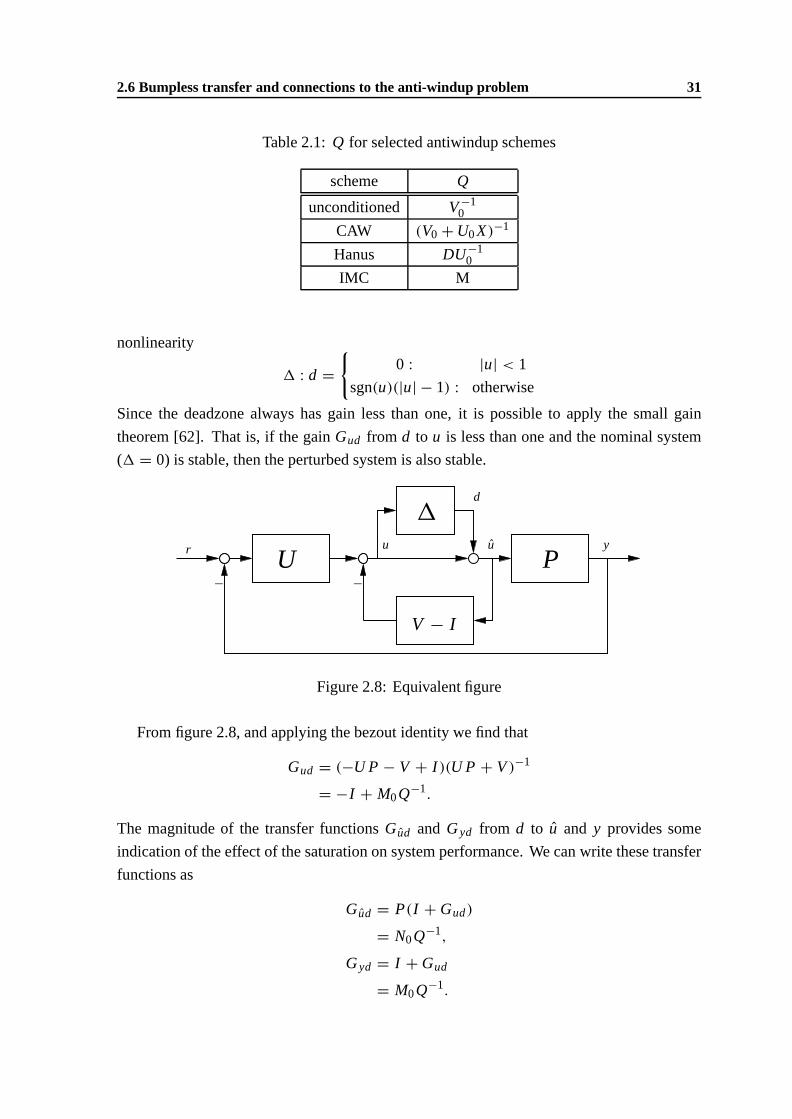
Note that when the nonlinearity8 is a unit saturation, then by rewriting the saturation as a
deadzone plus unity we obtain the equivalent picture shown in figure 2.8.1 is the deadzone
2.6 Bumpless transfer and connections to the anti-windup problem 31
Table 2.1:Q for selected antiwindup schemes
scheme Q
unconditioned V−10
CAW (V0+U0X)−1
Hanus DU−10
IMC M
nonlinearity
1 : d ={
0 : |u| < 1
sgn(u)(|u| − 1) : otherwise
Since the deadzone always has gain less than one, it is possible to apply the small gain
theorem [62]. That is, if the gainGud from d to u is less than one and the nominal system
(1 = 0) is stable, then the perturbed system is also stable.
U
V − I
u y
d
r
−−
u
1
P
Figure 2.8: Equivalent figure
From figure 2.8, and applying the bezout identity we find that
Gud = (−U P − V + I )(U P + V)−1
= −I + M0Q−1.
The magnitude of the transfer functionsGud and Gyd from d to u and y provides some
indication of the effect of the saturation on system performance. We can write these transfer
functions as
Gud = P(I + Gud)
= N0Q−1,
Gyd = I + Gud
= M0Q−1.

32 Preliminaries
In Miyamoto and Vinnicombe then, the design approach is to make the gainsGud andGyd
small (in terms of a weightedH∞ norm), while ensuring that theH∞ norm ofGud remains
less than 1. We will see in section 3.4.2 that this approach also results in guaranteed stability
and performance in a system with switching controllers and saturating actuators.
It should be noted that each of the schemes examined so far (including the generalized
schemes above), when applied to the bumpless transfer problem are equivalent to choosing
an appropriate controller statexK at each controller transition. This is clear, as each of
the schemes listed behaves according to the linear controller design immediately when the
controller in question is switched on.
QU0
QV0 − I
u yr
w1 w2
−−
u
8 P
Figure 2.9: Coprime factorization based scheme
2.7 Filtering and estimation
Estimation problems in control usually require estimating the state of a dynamical system from
noisy measurements of input and output data. Thefiltering estimation problem specifically
requires calculation of an estimate of the ’current’ state using data up to and including the
current time.
The Kalman filter [27] is an example of an optimal filter. That is, the estimatex of the
current statex is optimal with respect to the cost functionJ = E((x − x)T(x − x)), the
expectation of the squared error.
We will present here the Kalman filter equations for discrete and continuous-time time-
varying state-space systems, with inputs and outputs corrupted by zero-mean Gaussian noise.
The initial state estimate is also assumed to be taken from a Gaussian distribution with known
mean and variance.
2.7 Filtering and estimation 33
vw
uy
P
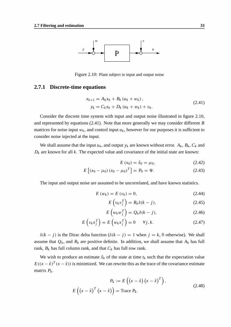
Figure 2.10:Plant subject to input and output noise
2.7.1 Discrete-time equations
xk+1 = Akxk + Bk (uk +wk) ,
yk = Ckxk + Dk (uk +wk)+ vk.(2.41)
Consider the discrete time system with input and output noise illustrated in figure 2.10,
and represented by equations (2.41). Note that more generally we may consider differentB
matrices for noise inputwk, and control inputuk, however for our purposes it is sufficient to
consider noise injected at the input.
We shall assume that the inputuk, and outputyk are known without error.Ak, Bk, Ck and
Dk are known for allk. The expected value and covariance of the initial state are known:
E (x0) = x0 = µ0, (2.42)
E[(x0− µ0) (x0− µ0)
T] = P0 = 9. (2.43)
The input and output noise are assumed to be uncorrelated, and have known statistics.
E (wk) = E (vk) = 0, (2.44)
E(vkv
Tj
)= Rkδ(k− j ), (2.45)
E(wkw
Tj
)= Qkδ(k− j ), (2.46)
E(vkxT
j
)= E
(wkxT
j
)= 0 ∀ j , k. (2.47)
δ(k − j ) is the Dirac delta function (δ(k − j ) = 1 when j = k, 0 otherwise). We shall
assume thatQk, andRk are positive definite. In addition, we shall assume thatAk has full
rank,Bk has full column rank, and thatCk has full row rank.
We wish to produce an estimatexk of the state at timetk such that the expectation value
E((x− x)T (x− x)) is minimized. We can rewrite this as the trace of the covariance estimate
matrix Pk.
Pk := E((
x − x) (
x − x)T)
,
E((
x − x)T (
x − x)) = TracePk.
(2.48)

34 Preliminaries
Given the state estimate at the previous time stepxk−1, a natural initial estimate forxk is:
x′k = Ak−1xk−1+ Bk−1uk−1. (2.49)
Note that we have not yet used the output measured at timetk. We can then apply a
correction to the state estimate based on the error between the actual output and predicted
output. So a sensible estimate is:
xk = x′k + Kk
[yk − Ckx
′k − Dkuk
]= (Ak−1− KkCk Ak−1) xk−1+ (Bk−1− KkCkBk−1) uk−1+ Kkyk − Kk Dkuk,
(2.50)
where the gainKk is to be determined.
Theorem 2.7.1.Consider the linear discrete time system(2.41), and the linear state es-
timator (2.50). The optimal gainKk, which minimizes the least squares estimation error
E[(xk − xk)(xk − xk)
]T = TracePk is:
Kk = PkCTk
(DkQk DT
k + Rk)−1
(2.51)
where
Pk =(Ak−1Pk−1AT
k−1+ Bk−1Qk−1BTk−1
)−1+ CTk
(DkQk DT
k + Rk)−1
Ck (2.52)
Proof. The proof of the theorem in this particular form appears in [47], adapted from proofs
in Sorenson [52], and Stengel [54].
Hence, the Kalman filter can be implemented in recursive form with the three equations
xk = (Ak−1− KkCk Ak−1) xk−1+ (Bk−1− KkCk Bk−1) uk−1+ Kkyk − Kk Dkuk, (2.53)
Kk = PkCTk
(DkQk DT
k + Rk)−1
, (2.54)
Pk =(Ak−1Pk−1AT
k−1+ Bk−1Qk−1BTk−1
)−1+ CTk
(DkQk DT
k + Rk)−1
Ck, (2.55)
along with the boundary conditionsP0 = 9 andx0 = µ0.
The equations may be simplified further if the system observed, and the noise statistics
are time-invariant. In that case the equations reduce to
xk = (A− KC A) xk−1+ (B− KC B)uk−1+ K yk − K Duk, (2.56)
K = PCT (DQDT + R)−1
, (2.57)
P = (AP AT + B QBT)−1+ CT (DQDT + R)−1
C. (2.58)
Since the matricesK andP are now constant, they may be precomputed allowing for very
simple and computationally efficient observer form implementation of the filter.

2.8 The deterministic filtering problem 35
2.7.2 Continuous-time equations
Now consider the estimation problem for a continuous-time plant. The signals of figure 2.10,
and the state-space equations are now continuous-time.
x(t) = A(t)x(t)+ B(t) (u(t)+ w(t)) ,y(t) = C(t)x(t)+ D(t) (u(t)+ w(t))+ v(t). (2.59)
Once again, the expected valueµ0 and covariance9 of the initial state are known, as are
the statistics of the input and output noise.
E (w(t)) = E (v(t)) = 0, (2.60)
E(v(t)vT(s)
) = R(t)δ(t − s), (2.61)
E(w(t)wT (s)
) = Q(t)δ(t − s), (2.62)
E(v(t)xT(s)
) = E(w(t)xT (s)
) = 0 ∀ t, s. (2.63)
Under these assumptions, we can again compute the equations for the optimal (with respect
to the expectation of the squared state error) Kalman filter.
The resulting equations (not derived here) are:
˙x(t) = (A(t)− K (t)C(t)) x(t)+ (B(t)− K (t)D(t)) u(t)+ K (t)y(t), (2.64)
K (t) = P(t)CT(t)(D(t)Q(t)DT(t)+ R(t)
)−1, (2.65)
P(t) = P(t)AT(t)+ A(t)P(t)+ B(t)Q(t)BT(t)
− P(t)CT (t)(D(t)Q(t)D(t)T + R(t)
)−1C(t)P(t),
(2.66)
along with the boundary conditionsP(0) = 9 andx(0) = µ0.
In the time-invariant case, the equations are:
˙x(t) = (A− KC) x(t)+ (B− K D)u(t)+ K y(t), (2.67)
K = PCT (DQDT + R)−1
, (2.68)
0= P AT + AP+ B QBT − PCT (DQDT + R)−1
C P. (2.69)
2.8 The deterministic filtering problem
We now consider an alternative perspective to the standard form of the state estimation.
Rather than making stochastic assumptions about the noise signalsw andv, we simply find

36 Preliminaries
the state-estimate which corresponds to minimization of a quadratic cost function of the
noise signals and the initial state. We show that with appropriate identifications, the result
of this deterministic filteringproblem is identical to the optimal Kalman filter estimate with
stochastic assumptions.
This approach was first used by Bertsekas and Rhodes in [5], estimating the state of a
dynamical system with no control input.
2.8.1 Continuous-time equations
Consider the arrangement of figure 2.10, described by equations (2.59).
In the deterministic filtering problem, we wish to find the estimatex(t) of the statex(t),
which corresponds with initial statex(t0), and noise signalsw(t) andv(t) which minimize
the quadratic cost function
J(t) = (x(t0)− µ0)T9(x(t0)− µ0)+
∫ t
t0
(wT (s)Q(s)w(s)+ vT(s)R(s)v(s)
)ds (2.70)
Theorem 2.8.1.Assume that the signalsu and y are known and defined over the interval
[t0, t]. Then, the optimal estimatex(t) of the state of system(2.59)at timet with respect to
the cost function(2.70)may be obtained by solving the differential system
˙x(t) = (A(t)− K (t)C(t)) x(t)+ (B(t)− K (t)D(t))u(t)+ K (t)y(t), (2.71)
K (t) = P(t)CT (t)(D(t)Q(t)DT (t)+ R(t)
)−1, (2.72)
P(t) = P(t)AT (t)+ A(t)P(t)+ B(t)Q(t)BT(t)
− P(t)CT(t)(D(t)Q(t)D(t)T + R(t)
)−1C(t)P(t),
(2.73)
with the boundary conditionsP(0) = 9 and x(0) = µ0.
This result (and the discrete time version) is obtained directly from Bertsekas and Rhodes
main result in [5]. The approach is to treat the problem as an optimal tracking problem
in reverse time. The noise signalw(t) is treated as the ‘control’ input, and the boundary
condition is on the initial state rather than the final error. A direct dynamic programming
solution is also contained in [14].
2.8.2 Discrete-time equations
The discrete-time solution is obtained in similar fashion to the continuous case. We solve an
optimization problem with respect to the cost function
Jk = (x0− µ0)T9(x0 − µ0)+
k∑i=0
(wT
i Qiwi + vTi Ri vi
)(2.74)

2.8 The deterministic filtering problem 37
Theorem 2.8.2.Assume that the signalsu and y are known and defined over the interval
[0, k]. Then, the optimal estimatexk of the state of system(2.41)at timek with respect to the
cost function(2.74)may be obtained by solving the difference equations
xk = (Ak−1− KkCk Ak−1) xk−1+ (Bk−1− KkCk Bk−1) uk−1+ Kkyk − Kk Dkuk, (2.75)
Kk = PkCTk
(DkQk DT
k + Rk)−1
, (2.76)
Pk =(Ak−1Pk−1AT
k−1+ Bk−1Qk−1BTk−1
)−1+ CTk
(DkQk DT
k + Rk)−1
Ck, (2.77)
with the boundary conditionsP0 = 9 and x0 = µ0.
These results allow us to use the simplicity of Kalman filter implementations to solve
problems which can be described in terms of two-norm noise minimization. We apply the
results to the problem of optimal initial state selection for switching controllers in chapter 4.

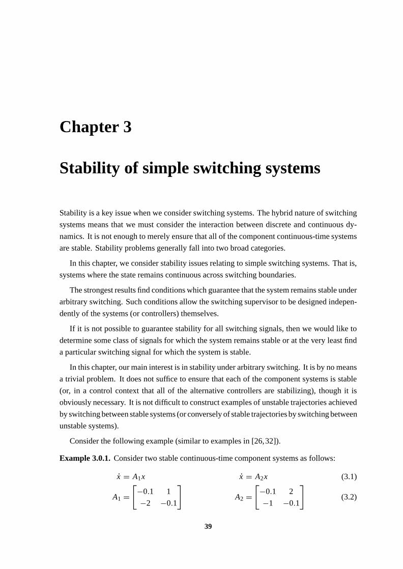
Chapter 3
Stability of simple switching systems
Stability is a key issue when we consider switching systems. The hybrid nature of switching
systems means that we must consider the interaction between discrete and continuous dy-
namics. It is not enough to merely ensure that all of the component continuous-time systems
are stable. Stability problems generally fall into two broad categories.
In this chapter, we consider stability issues relating to simple switching systems. That is,
systems where the state remains continuous across switching boundaries.
The strongest results find conditions which guarantee that the system remains stable under
arbitrary switching. Such conditions allow the switching supervisor to be designed indepen-
dently of the systems (or controllers) themselves.
If it is not possible to guarantee stability for all switching signals, then we would like to
determine some class of signals for which the system remains stable or at the very least find
a particular switching signal for which the system is stable.
In this chapter, our main interest is in stability under arbitrary switching. It is by no means
a trivial problem. It does not suffice to ensure that each of the component systems is stable
(or, in a control context that all of the alternative controllers are stabilizing), though it is
obviously necessary. It is not difficult to construct examples of unstable trajectories achieved
by switching between stable systems (or conversely of stable trajectories by switching between
unstable systems).
Consider the following example (similar to examples in [26,32]).
Example 3.0.1.Consider two stable continuous-time component systems as follows:
x = A1x x = A2x (3.1)
A1 =[−0.1 1
−2 −0.1
]A2 =
[−0.1 2
−1 −0.1
](3.2)
39

40 Stability of simple switching systems
−0.2 −0.15 −0.1 −0.05 0 0.05 0.1 0.15 0.2−0.2
−0.15
−0.1
−0.05
0
0.05
0.1
0.15
0.2
(a) f1 trajectory
−0.2 −0.15 −0.1 −0.05 0 0.05 0.1 0.15 0.2−0.2
−0.15
−0.1
−0.05
0
0.05
0.1
0.15
0.2
(b) f2 trajectory
Figure 3.1:
f1 = A1x, and f2 = A2x are both stable dynamical systems. Figure 3.1 shows trajectories
for f1 and f2 respectively, with the initial conditionx = [0.1 0.1]∗.Suppose we switch between these systems according to regions in the state space. Let
x =[
x1
x2
]. Then let us switch at the boundariesx1 = 0 andx2 = 0 such thatf1 = A1x is
active in quadrants 2 and 4 (x1x2 < 0) of the state space, andf2 = A2x active in quadrants
1 and 3 (x1x2 ≥ 0). Figure 3.2 shows the resulting unstable trajectory.
We can construct a similar example in a plant and controller context as follows.
Example 3.0.2.Consider the feedback arrangement depicted in figure 3.3. PlantP (with zero
through term), and controllersK1 andK2 are given by a particular state space representations
G =[
A B
C 0
]K1 =
[A1 B1
C1 D1
]K2 =
[A2 B2
C2 D2
]PlantG has statexG, and controllerKi has statexKi (i = {1, 2}).
Then, we have a switching system between the closed loop systems[xG
˙xKi
]=[
A+ B Di C BCi
Bi C Ai
][xG
xKi
]i = 1, 2. (3.3)
Now if we choose
G =[
0.5 1
1 0
]K1 =
[−0.1 −1
2 −0.6
]K2 =
[−0.6 −1.5
1.5 −0.1
],
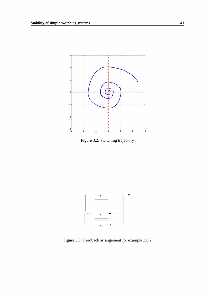
Stability of simple switching systems 41
−3 −2 −1 0 1 2 3−3
−2
−1
0
1
2
3
Figure 3.2: switching trajectory
P
K1
K2
Figure 3.3: Feedback arrangement for example 3.0.2

42 Stability of simple switching systems
−0.2 −0.15 −0.1 −0.05 0 0.05 0.1 0.15 0.2−0.2
−0.15
−0.1
−0.05
0
0.05
0.1
0.15
0.2
(a) f1 trajectory
−0.2 −0.15 −0.1 −0.05 0 0.05 0.1 0.15 0.2−0.2
−0.15
−0.1
−0.05
0
0.05
0.1
0.15
0.2
(b) f2 trajectory
Figure 3.4:
we obtain the closed loop equations[xG
˙xK1
]=[−0.1 2
−1 −0.1
][xG
xK1
], and (3.4)[
xG
˙xK2
]=[
0.4 1.5
−1.5 −0.6
][xG
xK2
]. (3.5)
Thus the closed loop dynamics are stable foci about the origin, with the same direction of
flow, and orientation 45◦ apart. Figure 3.4 shows the respective closed loops applied without
switching, and with initial states[xG xKi
]∗ = [0.1 0.1]∗
.
Suppose we employ an autonomous switching scheme such that controllerK1 is employed
when the plant state satisfies the constraint|x| ≤ 0.1, andK2 otherwise. Then trajectories
beginning from initial states close to the origin will converge, however for large enough
initial conditions, the trajectory will converge to a limit cycle. Figure 3.5 shows the switching
trajectory beginning with initial state[xG xKi
]∗ = [0.1 0.1]∗
(i = 2).
In this chapter we will consider stability issues for simple switching systems By that we
mean switching systems in which the state is continuous across switching times.
3.1 Common Lyapunov functions for switching systems
It is a relatively straightforward observation that, given a family of vector fields
x(t) = fi (x(t)), i ∈ I , x(t) ∈ Rn (3.6)
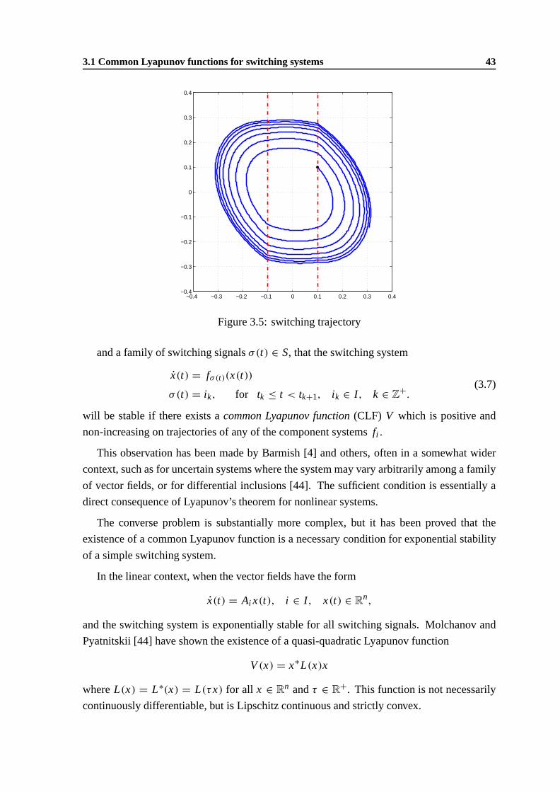
3.1 Common Lyapunov functions for switching systems 43
−0.4 −0.3 −0.2 −0.1 0 0.1 0.2 0.3 0.4−0.4
−0.3
−0.2
−0.1
0
0.1
0.2
0.3
0.4
Figure 3.5: switching trajectory
and a family of switching signalsσ(t) ∈ S, that the switching system
x(t) = fσ(t)(x(t))
σ (t) = i k, for tk ≤ t < tk+1, i k ∈ I , k ∈ Z+. (3.7)
will be stable if there exists acommon Lyapunov function(CLF) V which is positive and
non-increasing on trajectories of any of the component systemsfi .
This observation has been made by Barmish [4] and others, often in a somewhat wider
context, such as for uncertain systems where the system may vary arbitrarily among a family
of vector fields, or for differential inclusions [44]. The sufficient condition is essentially a
direct consequence of Lyapunov’s theorem for nonlinear systems.
The converse problem is substantially more complex, but it has been proved that the
existence of a common Lyapunov function is a necessary condition for exponential stability
of a simple switching system.
In the linear context, when the vector fields have the form
x(t) = Ai x(t), i ∈ I , x(t) ∈ Rn,
and the switching system is exponentially stable for all switching signals. Molchanov and
Pyatnitskii [44] have shown the existence of a quasi-quadratic Lyapunov function
V(x) = x∗L(x)x
whereL(x) = L∗(x) = L(τx) for all x ∈ Rn andτ ∈ R+. This function is not necessarily
continuously differentiable, but is Lipschitz continuous and strictly convex.

44 Stability of simple switching systems
Dayawansa and Martin [10] have proved a similar necessity theorem, but have additionally
shown that a continuously differentiable Lyapunov functionV may be obtained by smoothing
a similarly obtained quasi-quadratic function.
Theorem 3.1.1 ( [10]).The linear simple switching system is uniformly exponentially stable
if and only if there exists a continuously differentiable functionV : Rm → R such that
V(x) = ∇V(x)Ai x is negative definite for alli ∈ I .
It is important to note that it is not in general possible to construct common quadratic Lya-
punov functions. Dayawansa gives an example of a uniformly exponentially stable switching
system (with two linear component systems) which does not admit a common quadratic
Lyapunov function.
If the index setI is finite, and a common quadratic Lyapunov function exists, it can be
found by solving forP > 0 andQ > 0 the system of inequalitiesA∗i P+ P Ai < −Q for all
i ∈ I .
Dayawansa and Martin also extend the result to nonlinear systems which are globally
asymptotically stable and locally uniformly exponentially stable.
3.2 Multiple Lyapunov functions
Peleties and DeCarlo [48], and Michael Branicky in [7] introduce a somewhat different
approach for analysing stability of a switching system. The basic idea is to findLyapunov-
like functionsVi for each of the component vector fields, which are positive definite and
decreasing whenever thei ’th loop is active. We then ensure stability for a family of switching
signalsSby ensuring thatVi is non-increasing on an appropriate sequence of switching times.
The multiple Lyapunov function stability condition is, in a sense weaker than the common
Lyapunov function approach when applied to the problem of stability for all switching signals.
The multiple function approach can however be more tractable in some cases, especially when
considering restricted classes of switching signals when stability cannot be guaranteed for
arbitrary switching.
In considering the multiple Lyapunov function approach, we shall modify the definition
of switching signals to include the system initial conditions. This allows for the study of
stability for systems where the set of possible switching signals at any point is dependent
upon the state of the system at that point. For example, we may consider piecewise affine
hybrid system under this framework (see for example [26]).
Definition 3.2.1. An anchoredswitching signal is a pair(x0, σ ) wherex0 ∈ Rn is an initial
state, andσ : R+ → I is a (non-zeno) piecewise constant switching signal.

3.2 Multiple Lyapunov functions 45
We shall let the class of anchored switching signals under consideration beS, and assume
the family of vector fields is finite (letI = {1, 2, . . . , N}). Fix a particular signal(x0, σ ) ∈ S,
with associated switching times{tk} and indices{i k} (σ(t) = i k whentk ≤ t < tk+1).
Consider the family of vector fields 3.6, or the equivalent discrete-time family
x(k+ 1) = fi (x(k)), i ∈ I
Given a particular switching sequenceσ , let σ |n be the sequence of endpoints of the
intervals for which then’th system is active. That is:
σ |n = {tk : i k = n, or i k−1 = n}
The interval completionof a time sequenceT = t0, t1, t2, ... is the set
I(T) =∞⋃
k=0
(t2k, t2k+1)
Thus,I(σ |n) is the set of times for which then’th system is active.
Let E(T) = {t0, t2, t4, . . .} denote theeven sequenceof T. Then,E(σ |n) is the set of times
at which then’th system is engaged.
Definition 3.2.2. Given a strictly increasing set of timesT in R, a functionV is said to be
Lyapunov-likefor a hybrid trajectoryφσ (.) over a time sequenceT if it satisfies the following:
• V is a continuous, positive definite, and radially unbounded function with continuous
partial derivatives
• V(0) = 0
• V(x(t)) ≤ 0 for all t ∈ I(T)
• V is monotonically non-increasing onE(T)
The following is a version of Branicky’s theorem. We will not prove the result here, since
an extension of the theorem is proved in chapter 6.
Theorem 3.2.1 ( [7]). Consider a set of vector fields(3.6). Let S be the set of anchored
switching sequences associated with the system.
If there exist functionsVi such that over all anchored switching sequences(x0, σ ) ∈ S, Vi
is Lyapunov-like for the hybrid trajectory overσ |i , then the switching system(3.7) is stable
in the sense of Lyapunov.

46 Stability of simple switching systems
111 2 2 111 2 2
Figure 3.6: Multiple Lyapunov functions forN = 2
Additionally, the system is asymptotically stable if for someεi andδi
Vi (x(t)) < −εi ‖x(t)‖2
for t in I(σ |i ), andVi are strictly decreasing onE(σ |i ):Vi (x(tk))− Vi (x(t j )) < −δi
∥∥x(t j )∥∥2, (3.8)
wheret j < tk, andi j = i k = i .
We will refer to (3.8) as thesequence decreasingcondition. This is not precisely the same
as the asymptotic stability conditions presented by Branicky [7] and Pelleties [48], but it is
perhaps the most useful expression for our purposes.
Figure 3.6 illustrates a possible sequence of multiple Lyapunov functions for a 2-switched
system which satisfies the (respectively Lyapunov stability and asymptotic stability) condi-
tions for theorem 3.2.1. The black lines denoteV1, and the red lines denoteV2. The solid
lines show the active Lyapunov function.
The multiple Lyapunov function approach may be used in order to restrict the set of
admissible switching signals in order to ensure stability.
3.3 Dwell time switching
3.3.1 If we are switching between stable vector fields, it is fairly obvious that stability of
a simple switching system can be guaranteed if we switch sufficiently slowly. That is, we
find can find aτ such that if wedwell at each vector field for at least timeτ then stability is
guaranteed. This approach to stabilizing switching systems is known asdwell timeswitching,
and was introduced by Morse in [46]. The selectedτ is known as the systemdwell time.
The approach there is as follows. Each component vector field is stable, so there exist
functionsVi for eachi ∈ I which satisfy the inequalities
ai ‖x‖2 ≤ Vi (x) ≤ bi ‖x‖2

3.3 Dwell time switching 47
and
∇Vi (x) fi (x) ≤ −ci ‖x‖2
for some constantsai , bi andci . Therefore we can write
∇Vi (x) fi (x) ≤ −λi Vi (x)
whereλi = ci /bi . This gives the exponential upper bound onVi of
Vi (x(t0+ τ) ≤ e−λi τVi (x(t0)),
provided thatσ(t) = i for t ∈ [t0, t0+ τ)Now consider beginning with thei k’th loop active at some timetk, and switching to the
i k+1’th loop at timetk+1. This results in the set of inequalities
aik
bik+1
Vik+1(x(tk+1)) ≤ aik ‖x(tk+1)‖2 ≤ Vik(x(tk+1)) ≤ e−λik (tk+1−tk)Vik(x(tk)).
Hence, if the time gap(tk+1− tk) satisfies
tk+1− tk >−1
λi kln
(aik
bik+1
)then the sequence non-increasing condition
Vik+1(x(tk+1)) < Vik(x(tk))
is satisfied for that switch. Thus if we choose the dwell timeτ to be
τ ≥ supi, j
(−1
λiln
(ai
bj
)),
then the sequence non-increasing condition can be satisfied for all possible switches.
This approach is obviously potentially conservative,both because of the ’spherical’ bounds
used in the calculations, and because the choice of Lyapunov function is arbitrary. In the fol-
lowing section, we examine a refinement of the technique for the case of quadratic Lyapunov
functions.
3.3.1 Dwell times for linear simple switching systems
Here we consider an approach to dwell time switching which makes use of the elliptical
bounds on trajectories which are provided when we have quadratic Lyapunov functions.

48 Stability of simple switching systems
Let us illustrate the principal idea forN = 2. Suppose we have Lyapunov functions
V1 = x∗P1x, and V2 = x∗P2x, where P1 > 0 and P2 > 0 are solutions to Lyapunov
equations
A∗1P1+ P1A1 = −Q1
A∗2P2+ P2A2 = −Q2
for some positive definiteQ1 andQ2.
Let the initial conditions bex0 at timet0, with σ(t0) = 1. Now we know that the trajectory
is bounded by the level setx∗P1x = x0P1x0 while vector field 1 is active. Suppose we switch
from loop 1 to loop 2 at timet1, and then back to loop 1 at timet2. If A1 is stable, then we
know that
x(t1)∗P1x(t1) < x∗0 P1x0
From the matrixQ1, it is possible to derive an exponential upper bound on the decay of
V1 after some timeτ .
Lemma 3.3.1.SupposeV(x(t)) = x(t)∗Px(t) whereP > 0 is the solution to the Lyapunov
equation
A∗P + P A= −Q
for someA and Q > 0. Then the value of the function at timet0+ τ satisfies the bound
V(x(t0+ τ)) ≤ e−λτV(x(t0))
whereλ is the minimum eigenvalue of the matrixP−1Q.
Proof. The bound is calculated, by calculating the maximum value of the derivativeV on a
particular level curve ofV .
Consider the level curvex∗Px = a. The maximum value ofV on this curve, is
−minx(x∗Qx) such thatx∗Px = a.
Geometrically, this corresponds to finding the numberb such that the level curvex∗Qx = b
fits exactly inside the level curvex∗Px = a (see figure 3.7).
Consider a transformationz= T x such that the level curvex∗Px = a is transformed into
the circlez∗z = a. This is obtained by the Cholesky factorizationP = T∗T , and it exists
precisely whenP is positive definite.
So now we wish to find
minz
(z(T∗)−1QT−1z
)such thatz∗z= a.

3.3 Dwell time switching 49
level curvex∗Qx = b
level curvex∗Px = a
minx(x∗Qx) s.t x∗Qx = b
Figure 3.7: Geometrical illustration
This is simplya times the minimum eigenvalue of the matrix(T∗)−1QT−1 (or equivalently,
the minimum eigenvalue ofP−1Q). Thus we now have the bound
V ≤ −λV
whereλ is the minimum eigenvalue of the matrixP−1Q (since eigenvalues are transpose-
invariant). Hence
V(x(t0+ τ) ≤ e−λτV(x(t0))
Note that this calculation, based on elliptical bounds is strictly less conservative than the
spherical bounds considered in the previous section.
Thus at the timet1, we have the bound
x(t1)∗P1x(t1) ≤ e−λ1(t1−t0)x∗0 P1x0
whereλ1 is calculated using lemma 3.3.1. We can also now calculate the maximum value of
the Lyapunov functionV2 on the level curve
x∗P1x = e−λ1(t1−t0)x∗0 P1x0,
using a similar technique to that employed in lemma 3.3.1. That is,
maxx(x∗P2x) such that x∗P1x = e−λ1(t1−t0)x∗0 P1x0
= k12e−λ1(t1−t0)x∗0 P1x0,

50 Stability of simple switching systems
wherek12 is the maximum eigenvalue ofP−11 P2.
Thus we now have the bound
V2(x(t1)) ≤ k12e−λ1(t1−t0)V1(x(t0)).
We continue in the same fashion through the decay ofV2 to t2, and at the switch back to loop
1, resulting in the bound
V1(x(t2)) ≤ k12k21e−λ1(t1−t0)e−λ2(t2−t1)V1(x(t0)),
whereki j is the maximum eigenvalue ofP−1i Pj , andλi is the minimum eigenvalue ofP−1
i Qi .
Thus we can guarantee the sequence decreasing condition if the dwell timeτ is chosen such
that
k12k21e−(λ1+λ2)τ < 1.
That is, we use
τ >1
λ1+ λ2ln (k12k21) .
In the generalN loop case, the required dwell time is a supremum of such a form, but over
arbitrary sequences of switches.
Let us defineL [N] to be the set of all cycles of elements of{1, 2, . . . , N}. That is,
l ∈ L [N] is a finite sequence beginning and ending with the same element, with no repeated
element (except for the first/last). Note thatL [N] can be thought of as the set of all cycles
of KN , the complete graph withN vertices (see [17] for example). If we can ensure that each
Vi is decreasing on all such cycles, then stability may be guaranteed via theorem 3.2.1.
We shall use the notationi ∈ l to mean ‘the elementi appears in the cyclel ’.
As a slight abuse of notation, we shall usei j ∈ l to mean the sequence{i, j } appears in
l in that particular order. Whenl is a cycle of switching sequence indices, this means that a
switch from statei to statej occurs in the switching sequence.
Consider a finite family of stable linear vector fields
x = Ai x,
with corresponding Lyapunov functionsVi = x∗Pi x for i ∈ {1, 2, . . . , N}. The Pi > 0
satisfy the Lyapunov equations
A∗i Pi + Pi Ai = −Qi
for Qi > 0.

3.3 Dwell time switching 51
Theorem 3.3.2.Letki j be the maximum eigenvalue ofP−1i Pj , andλi the minimum eigenvalue
of P−1i Qi .
If we chooseτ such that
τ > supl∈L [N]
1∑i∈l λi
ln
∏i j ∈l
ki j
, (3.9)
then the simple switching system
x = Aσ(t)x,
σ (t) = i k, ∀ tk ≤ t < tk+1, i k ∈ {1, 2, . . . , N}, k ∈ Z+, (3.10)
is guaranteed to be stable for all switching sequences with a minimum dwell time ofτ .
Proof. Consider a particular switching sequence
σ(t) = i k, for tk ≤ t < tk+1,
where the sequence of switching times satisfiestk+1− tk > τ for all k. Suppose the switching
sequence contains a loop (possibly with repeated elements)l , beginning with them’th vector
field. Then, the ‘gain’ ofVm from the beginning to the end of the loop is bounded above by∏i j ∈l
ki j
e−(∑
i∈lλi
)τ
.
This is clear, since we have already shown thatki j represents the maximum gain from one
Lyapunov function to another at a switch, ande−λi τ represents the minimum decay in the
value ofVi while in thei ’th state.
Furthermore, for any arbitrary loop (which may contain repeated elements), this expression
can be factored into similar expressions for non-repeating loops. For example
k12k23k32k21e−(λ1+λ2+λ3+λ2)τ =
(k12k21e
−(λ1+λ2)τ) (
k23k32e−(λ2+λ3)τ
).
Hence, ifτ is chosen such that
τ >
1∑i∈l λi
ln
∏i j ∈l
ki j
for each non-repeating loopl , then∏
i j ∈lki j
e−(∑
i∈lλi
)τ
< 1
for each non-repeating loop, and hence also for repeating loops. Thus the decreasing con-
dition from theorem 3.2.1 for asymptotic stability is satisfied, and the switching system is
asymptotically stable.

52 Stability of simple switching systems
There is clearly still some conservatism in this result, arising from the fact that it is
dependent on particular choices ofPi .
An upper bound on this minimum dwell-time (but a less complex calculation) is the choice
τ > supi∈l
(1
λi
)supi j ∈l
(ln(ki j)). (3.11)
This will in fact ensure the inequality
Vik+1(x(tk+1)) < Vik(x(tk))
is satisfied for allk. This is a stronger condition than our decreasing condition in theorem 3.2.1,
but is the same as the condition for asymptotic stability used in [7].
3.4 Choice of controller realizations
Switching between stabilizing controllers for a given plant does not in general ensure stabil-
ity of the resulting trajectory. It is possible, however to choose realizations for stabilizing
controllers such that stability can be guaranteed.
3.4.1 IMC approach
Recent work by Hespanha and Morse [25] uses an Internal Model Control framework in
order to choose realizations for given controller such that stability of the switching system is
guaranteed.
The result is based on the following lemma, and the Youla parameterization of stabilizing
controllers [62].
Lemma 3.4.1.Given any finite family of asymptotically stable transfer matricesP = {Pi :i ∈ I } with McMillan degree no larger thann, and anyn × n symmetric positive definite
matrixQ, there exist stabilizable and detectable realizations{Ai , Bi ,Ci , Di } for eachPi ∈ P
such that
Q Ai + A∗i Q < 0
for all i ∈ I .
Proof. Suppose{ Ai , Bi , Ci , Di } is any realization forPi . Then, we can find matricesQi
satisfying
Qi Ai + A∗i Qi = −Xi (3.12)

3.4 Choice of controller realizations 53
for eachi , with Xi positive definite. In fact, we can chooseQi such thatQ− 12 Q
12i is full rank
for eachi . Given positive definite matricesQ and Qi , we can writeQ = (Q12)∗Q1
2 and
Qi = (Q12i )∗Q
12i . Define
Ai = Q−12 Q
12i Ai Q
− 12
i Q12 , Bi = Q−
12 Q
12i Bi , Ci = Ci Q
− 12
i Q12 , Di = Di
Now we can rewrite equation (3.12) as
(Q−12 Q
12i )∗(Q Ai + A∗i Q)(Q−
12 Q
12i ) = −I ,
and hence
Q Ai + A∗i Q = −(Q−12
i Q12)∗Q−
12 Q
12 < 0.
This result means that for any family of stable linear dynamical systems, we can construct
realizations such that a simple switched system will be stable for any switching signalσ .
Obviously, in a plant/controller framework, it is only possible to choose the realization of the
controller and not the plant. Hespanha overcomes this difficulty by using an Internal Model
Control framework [45], constructing a controller which contains an internal realization of
a particular closed loop transfer function, and a model of the plant. The realization of the
model of the closed loop transfer function can then be chosen according to lemma 3.4.1, and
stability will be guaranteed provided that all the models are exact.
3.4.2 Choice of coprime factorizations
We can consider another approach to the design of stabilizing switching control systems.
This approach is based on the ideas in Miyamoto and Vinnicombe [42] in the context of the
anti-windup problem.
Suppose we have a plantG, and a set of stabilizing controllersKi . We may choose a
right coprime factorization of the plantG = N M−1, and left coprime factorizations of the
controllersKi = V−1i Ui , such that for eachi the bezout identity
Vi M +Ui N = I
is satisfied [62, section 5.4]. Furthermore given anyQ such thatQ, Q−1 ∈ RH∞, the
factorizationsG = N M−1, andKi = V−1i Ui also satisfy the bezout identities
Vi M + Ui N = I ,
whereN = N Q, M = M Q, Ui = Q−1Ui , andVi = Q−1Vi .

54 Stability of simple switching systems
P
U1
I − V1
Ui
I − Vi
Un
I − Vn
w
v
u
u1
ui
un
Kσ
-
Figure 3.8: Switching arrangement
A particular choice ofQ for a controller factorization can also be thought of as a particular
choice for the plant factorization (viaQ), or vice versa. In the switching controller case, this
is true provided that all of the controllers have the same choice ofQ.
Now consider the coprime factor switching arrangement in figure 3.8. The switching con-
nection is such thatu(t) = uσ(t), whereσ(t) is the switching signal governing the controller
selection. The signalsu, v, andw are common to the loops. We can think of this system as
a plantP in a feedback loop with the augmented controllerKσ .
Note that for each loopi , we have
ui = (I − Vi )u− Ui Pu− Ui Pw + Ui v
= (I − Vi − Ui N M−1)u− Ui Pw + Ui v
= (M − Vi M − Ui N)M−1u− Ui Pw + Ui v
= (I − M−1)u− Ui Pw + Ui v.
Sinceu = uσ , we can write
u = (I − M−1)u− Uσ Pw + Uσ v
= −MUσ Pw + MUσ v
= −M(Uσ N)M−1w + MUσ v
= −M(I − Vσ M)M−1w + MUσ v
= −(I − MVσ )w + MUσ v,

3.4 Choice of controller realizations 55
U1
Ui
Vn
V1
Vi
Vn
M
N
w
v
u
y
Figure 3.9: Alternative view
and
y = P(u+ w)= N M−1((−(I − MVσ )w + MUσ v)+ w)= NVσw + NUσ v.
We assume that the signalsw andv are bounded with bounded two norm, and we know
all of the coprime factors are stable. Then the signalsVσw, Vσv, Uσw, andUσ v will all be
bounded with bounded two norm. Henceu andy are bounded with bounded two norm, and
the switching system is stable for all admissible switching sequences.
We can write these closed-loop relationships in the compact form[u
y
]=[−(I − MVσ ) MUσ
NVσ NUσ
][w
v
].
The arrangement can be illustrated as shown in figure 3.9. The stability of this switching
system is guaranteed sinceM, N, and eachUi andVi are stable. Note that the states of the
controllers evolve identically irrespective of which controller is active.
The implementation of this arrangement requires all of the controllers (in coprime factor
form) to be running even when not active. This corresponds closely with the coprime factor

56 Stability of simple switching systems
based schemes discussed in section 2.6 for both the antiwindup and bumpless transfer prob-
lems. The total state-space required has order equal to the sum of the orders of the coprime
factor controllers plus the order of the plant.
In fact, we will see later (section 6.4) that adding a reset structure to such controllers can
remove the need to run all of the off-line controllers, and also improve the performance of
the system.
In Miyamoto and Vinnicombe [42] and later work by Crawshaw and Vinnicombe [],
optimal anti-windup conditioning schemes are derived as a function of a chosen coprime
factorization of the plant, and implemented as a controller factorization. The result is that
the Youla parameterQ depends only on the plant, and so can be applied to any given LTI
controller.
3.5 Concluding remarks
We have discussed a number of important issues relating to the stability of simple switching
systems.
We have noted that a necessary and sufficient condition for stability of switching systems
under arbitrary switching is the existence of common Lyapunov functions.
Related work by Branicky shows that stability of a switching system over a given family of
switching signals may be proved viamultiple Lyapunov functions. This leads us to a means
of computing an upper bound on the minimum dwell time required to ensure stability of
switching systems (with fixed realizations).
We have observed that it is possible to ensure stability of a switching controller system by
choosing appropriate realizations for the controllers. Both of the methods discussed require
non-minimal implementations of the controllers in general. The IMC approach of Hespanha
generally requires controllers to be order 2nG+nKi , wherenG andnKi are the minimal orders
of the plant and controllers respectively. The coprime factor approach requires controllers
which are order max{nG, nKi }, however it also requires all controllers to be running when
off-line (increasing the effective order by a factor ofN, the number of controllers). We will
see in chapter 6 however, that we can remove the need to run all controllers by choosing an
appropriate initial state when controllers are switched on, while still retaining the stability
property (and further improving performance).

Chapter 4
Controller conditioning for switching
In this chapter we consider a performance problem with respect to a single controller switch.
The problem is solved via an optimization, which involves finding the controller state at a
switching time which most closely corresponds in some sense with the plant inputs and outputs
observed prior to the switch. We solve finite and infinite horizon optimizations in order to
obtain appropriate controller initializations in the switching context. We also show that the
solutions to these optimizations may, for certain weighting structures, be implemented via a
Kalman filter observer of the controller using the deterministic filtering results of chapter 2.
4.1 Controller state selection via a noise minimization prob-
lem
u2
u1
u yr GK
Figure 4.1: Generalized input substitution
Consider the general input substitution for the system illustrated in figure 4.1. We assume
that the plant is driven initially by the signalu1, and switches at some fixed time to the closed
57

58 Controller conditioning for switching
loop control signalu2 generated by the known controllerK in feedback with the plantP. The
signalu1 might come from manual control (a pilot), or an alternative automatic controller.
Initially, we will consider the regulator problem withr = 0. Later we will show how our
results fit into a reference tracking framework.
How do we determine a controller state at the switching time which will result in a smooth
transfer from the inputu1 to the controller inputu2? One way of interpreting transient signals
caused by controller switching, is that they are due in some sense to the mismatch between
the controller state at the switch, and the actual plant signals prior to the switch. If the signals
lie in the graph of the controller, and the controller is initialized correctly, there would beno
transient due to the switch at all.
A method of controller state selection therefore, is to measure the plant signals in the time
leading up to the switch, and find signals compatible with the off-line controller (in the graph
of the controller), which areclosein some sense to the observed signals. The controller state
corresponding to the “nearest” signals is then selected when the controller is switched on.
In other words, recast the setup of figure 4.2(a) into that of figure 4.2(b) (whereu andy
represent identical signals). We then find the hypothetical signalsu andy prior to the switch
such that
∥∥∥∥∥wv∥∥∥∥∥
2
is minimized (or some similar weighted norm).
uy yP
(a) System prior to switch
uy y u
w v
K
(b) Alternative view
Figure 4.2:
4.2 Discrete-time explicit solution
Consider now the discrete-time case, and assume that we switch from the external control
signal to the known feedback controllerK at timek = n. We can now write the equations

4.2 Discrete-time explicit solution 59
for the hypothetical controller in the loop prior tok = n as follows:
xk+1 = Axk + Byk,
uk = Cxk + Dyk,(4.1)
with xk ∈ Rs, {uk, uk, vk} ∈ Rp, and{yk, yk, wk} ∈ Rq. Iterating these equations, we can
write xn−k andyn−k, with k ≥ 0 in terms of the state at the switching instantxn.
xn−1 = A−1xn − A−1Byn−1,
xn−r = A−r xn −[
A−r B A−r+1B . . . A−1B]
yn−1
yn−2...
yn−r
,un−r = Cxn−r + Dyn−r
= C A−r xn −[C A−r B C A−r+1B . . . C A−1B− D
]
yn−1
yn−2...
yn−r
.
Let us denote byUr , Yr , Ur andYr ther step truncations of signalsu, y, u and y prior to
the switching timen expressed instackedform
Ur =
un−1
un−2...
un−r
Yr =
yn−1
yn−2...
yn−r
Ur =
un−1
un−2...
un−r
Yr =
yn−1
yn−2...
yn−r ,
and we can now write the (hypothetical) controller outputUr in terms of the state at time
k = n and the (hypothetical) controller inputYr
Ur = 0r xn − Tr Yr . (4.2)
0r is ther ’th step truncation of the reverse time impulse response, andT is ther by r

60 Controller conditioning for switching
Toeplitz matrix defined below
0r =
C A−1
C A−2
...
C A−r
,
Tr =
C A−1B− D 0 . . . 0
C A−2B C A−1B− D 0...
. . ....
C A−r B C A−r+1B . . . C A−2B C A−1B− D
.
Now we may define a weighted quadratic cost function
Jr =∥∥∥∥∥W
[Ur − Ur
Yr − Yr
]∥∥∥∥∥2
=[
Ur − Ur
Yr − Yr
]∗W∗W
[Ur − Ur
Yr − Yr
], (4.3)
and find the values ofUr , Yr , andxn which achieve the minimum.r defines the ‘horizon’ of
the optimization, and may be selected appropriately.
W is an arbitrary weighting matrix of appropriate dimension, which may be used to scale
signals in an appropriate way. It may also be used for example to include a ‘forgetting factor’,
which gives a higher priority to recently observed signals.
We may for instance, wish to optimize with respect to
Jr = α1(un−1− un−1
)2+ α2(un−2− un−2
)2+ . . .+ αr(un−r − un−r
)2+ β1
(yn−1− yn−1
)2+ . . .+ βr(yn−r − yn−r
)2 ≥ 0,
where
α1 ≥ α2 ≥ . . . αr > 0, and
β1 ≥ β2 ≥ . . . βr > 0.
This weight may be represented using the cost function (4.3), with
W =[
W1 0
0 W2
]> 0,
where
W1 = diag(√α1,√α2, . . . ,
√αr),
W2 = diag(√β1,
√β2, . . . ,
√βr
).

4.2 Discrete-time explicit solution 61
Theorem 4.2.1.For the discrete time dynamical system defined in(4.1) and given finite
signalsUr andYr , then the controller statexn which solves the minimum noise optimization
with respect to the cost function(4.3)and correspondingYr are given by:[Yr
xn
]=(
W
[−Tr 0r
I 0
])†
W
[Ur
Yr
]. (4.4)
Proof.
Jr =∥∥∥∥∥W
[Ur − Ur
Yr − Yr
]∥∥∥∥∥2
=∥∥∥∥∥W
[Ur + Tr Yr − 0xn
Yr − Yr
]∥∥∥∥∥2
=∥∥∥∥∥W
[Ur
Yr
]−W
[−Tr 0r
I 0
][Yr
xn
]∥∥∥∥∥2
,
so by standard least squares optimization (see appendix A)
argmin[Yrxn
] J =(
W
[−Tr 0r
I 0
])†
W
[Ur
Yr
], (4.5)
and
min[Yrxn
] J =[
Ur
Yr
]∗W∗
I −W
[−Tr 0
I 0
](W
[−Tr 0
I 0
])†W
[Ur
Yr
]. (4.6)
4.2.1 Scheme applied to basic example
Consider again the example of section 1.1.1. Using the least squares optimization procedure
illustrated above, we can select the controller initial state. The results are shown in figure 4.3.
The solid lines show the actual plant input and output for the simulation. The dotted lines
show the hypothetical controller input and output which lie closest to the observed signals in
the sense of the unweighted cost function (4.3). We can clearly see an improvement in the
transient response of the plant following the switch.
The norm of the signal following the switch is 12.92, compared to 17.46 for the uncon-
ditioned case. The improvement is evident to different degrees in examples with different
plants, and different prior signals.

62 Controller conditioning for switching
0 50 100 150 200 250 300 350 400 450 500−3
−2
−1
0
1
2
time
pla
nt
inp
ut
0 50 100 150 200 250 300 350 400 450 500−1
0
1
2
3
4
time
pla
nt
ou
tpu
t
(a) Unconditioned response
0 50 100 150 200 250 300 350 400 450 500−3
−2
−1
0
1
2
time
pla
nt
inp
ut
0 50 100 150 200 250 300 350 400 450 500−1
0
1
2
3
4
time
pla
nt
ou
tpu
t
actualhypothetical
actualhypothetical
(b) Conditioned response
Figure 4.3: Example
4.3 Kalman filter implementation
Suppose we wish to use a block diagonal weighting matrix
W = diag[Nn−1 Nn−2 . . . Nn−r Vn−1 . . . Vn−r
], (4.7)
where eachNi ∈ Rp×p andVj ∈ Rq×q is symmetric and positive definite.
In this case, the cost function (4.3) becomes
J =n−1∑
i=n−r−1
(w∗i W2
i wi + v∗i V2i vi
).
By making the identificationsx0 := xn−r−1, Rk = (V2k )−1, Qk = (N2
k )−1 and9−1 = 0,
we can form the identical cost function of the Deterministic Kalman Filter described in
section 2.8. As a result, we may directly apply a Kalman filter in order to obtain the controller
state at the switch which minimizes the hypothetical noise signalsw andv.
Theorem 4.3.1.The solution(4.4) to the weighted optimization with weighting matrix(4.7)
is equivalent to the solutionxn given by a Kalman filter (initialized at timen−r −1observing
the (hypothetical) noisy controller of figure 4.2(b) with “input”Ur and “output” Yr . The
filter has the parametersRk = (V2k )−1, Qk = (N2
k )−1 and9−1 = 0.
In this Kalman filter interpretation there is a free choice over the initial state of the filter,
which is the state at the beginning of the optimization horizonxn−r−1.

4.4 Implementation issues 63
4.4 Implementation issues
Wenow have two distinct ways of implementing this solution to thebumpless transferproblem.
One is via the controller reset defined by theorem 4.2.1, the other via the Kalman filter
implementation defined by theorem 4.3.1. We describe here briefly some of the differences
in the two approaches.
Clearly, the reset method requires direct access to the controller states, and ability to
manipulate these states. If we require an analogue implementation of the controller, then the
Kalman filter observer form implementation would be required.
If the reset method is used with a fixed optimization horizon length, the matrix(W
[−Tr 0r
I 0
])†
W
may be precomputed, so that the only on-line computation is a matrix multiplication with
matrices of the order of twice the optimization horizon. If the optimization horizon is a sig-
nificant length however, there may be significant computational advantages to implementing
the Kalman filter, since the order of the computations would be much lower.
There is a subtle distinction between the optimization horizons of the two methods. The
reset method has a fixed (and moving) horizon, always optimizing over a fixed time prior to
the switch. In the (finite horizon) Kalman filter case, the optimization will extend back to the
point at which the filter is switched on.
4.5 Time invariant equations
Suppose the controller to be switched on is time-invariant. Then, we may letAk = A, Bk = B,
Ck = C, andDk = D. Assume also that the optimization weighting is time-invariant.
Then, the solutions which are optimal in the infinite horizon may be obtained via the time-
invariant Kalman filter equations described in section 2.7. Though the switching performance
may be somewhat inferior for an infinite horizon optimization, the implementation of the
time invariant Kalman filter is very straightforward. The time invariant Kalman filter is
easily implemented in analogue hardware, allowing a wide array of applications for which
it may be more difficult to implement a time varying filter. The implementation of the time
invariant Kalman filter for conditioning of the controller state, is equivalent to the observer
controller implementation of figure 4.4, with constant observer gainH = AK. Let also
L = (DQD∗ + R). 8 is the switching nonlinearity.

64 Controller conditioning for switching
L−12 D
B− H D
A− HC
L−12Cdelay
H
u yr
−
u
8 P
Figure 4.4: Kalman filter observer controller
Figure 4.5 shows the results of the time invariant Kalman filter implemented for example
1. The norm of the input/output signals after the switch is 12.97, compared to 12.87 for
the optimization scheme with horizon 90 (and time varying Kalman filter), and compared to
17.46 for the unconditioned case.
0 50 100 150 200 250 300 350 400 450 500−1.5
−1
−0.5
0
0.5
1
1.5
2
time
plan
t inp
ut
0 50 100 150 200 250 300 350 400 450 500−1
0
1
2
3
4
time
plan
t inp
ut
Figure 4.5: Time invariant Kalman filter scheme
Convergence of the optimization scheme to the time invariant Kalman filter state selection
is illustrated in figure 4.6. The plot shows the norm of the difference between the controller
statexn selected by the Kalman filter, with the state selected by the optimization scheme (time
varying filter) for different horizon lengths.

4.6 Coprime factor representation 65
0 20 40 60 80 100 120 1400.1
0.2
0.3
0.4
0.5
0.6
0.7
0.8
Figure 4.6: Convergence of optimization scheme to time invariant Kalman filter
4.6 Coprime factor representation
The time-invariant Kalman filter observer form also may be represented as a left coprime
factorization of the controllerK = V−1U , where
[U V] =[
A− HC B− H D −H
L− 12C L− 1
2 D L− 12
]
The switch between controllers occurs in theI − V feedback loop as shown in figure 4.7.
This method of switching corresponds closely with the coprime factorization based anti-
windup methods (see section 2.6), with the nonlinearity (saturation or switch) placed in the
I − V feedback loop. This is an intuitively sensible arrangement, since the stability of the
coprime factors means that they will be stable if left to run open loop.
U
V − I
w1 w2
u
uext
y
r
−
uP
Figure 4.7: Coprime factorization form

66 Controller conditioning for switching
4.6.1 Special case weighting
Consider a time varying Kalman filter applied to a discrete-time LTI controller
K =[
A B
C D
]
in the infinite horizon, withD = 0.
The basic recursion equations are as follows
P−1k =
(APk−1A∗ + Qk−1
)−1+ C∗ (Rk)−1 C, (4.8)
Kk = PkC∗ (Rk)−1 . (4.9)
Suppose we choose a particular set of weighting matrices
Qk−1 = Q
fk, Rk = R
fk,
with Q, and R some constant matrices, andfk a scalar function ofk. Such a weighting
function may be described in the block diagonal form of equation (4.7).
Then we can write the state covariance matrixPk as follows
P−1k =
(APk−1A∗ + Q
fk
)−1
+ C∗(
R
fk
)−1
C
= fk(
A fk Pk−1A∗ + Q)−1+ fkC∗
(R)−1
C,
( fk Pk)−1 =
(A( fk Pk−1)A
∗ + Q)−1+ C∗ R−1C.
Now suppose we choose thefk such that
fkfk+1= λ,
with λ a constant. Now define
Pk = fk Pk.
Then we have
P−1k =
(A(
fkfk−1
Pk−1)A∗ + Q
)−1
+ C∗ R−1C
=(
A(λPk−1)A∗ + Q
)−1+ C∗ R−1C,

4.6 Coprime factor representation 67
and
Kk = PkC∗(Rk)−1
= Pk
fkC∗(
R
fk)−1
= PkC∗ R−1.
So we have an equivalent Kalman filtering problem with recursion equations
P−1k =
(APk−1 A∗ + Q
)−1+ C∗ R−1C, (4.10)
Kk = PkC∗ R−1. (4.11)
whereA = √λA.
Now sinceA, Q and R are constant then provided[A B
C 0
]is detectable, the Kalman filter equations (4.10) and (4.11) will converge to the time invariant
equations
P−1 =(
AP A∗ + Q)−1+ C∗ R−1C, (4.12)
K = PC∗ R−1. (4.13)
Thus, we can in fact implement an exponentially weighted infinite horizon optimization
problem with a time invariant Kalman filter with modifiedA matrix A = √λA, and modified
noise covariancesQ and R.
4.6.2 The reference problem
Let us now consider the general reference tracking problem (r 6= 0).
The methods of this chapter are based on the idea of keeping the state of the off-line
controllers compatible with signals which are close to the actual plant input and output. From
this perspective, it does not actually matter in determining the appropriate controller state
whether the current controller is operating with reference or not. The difficulty arises when
we wish to apply a reference to a new controller after a switch- we may observe potentially
large transient signals simply due to the reference itself.
The solution is to gently apply a new reference by filtering smoothly from an appropriately
chosen previous reference. We do not use the ’true’ reference, since, even if it were available

68 Controller conditioning for switching
U
V−1
w1 w2
yr uP
Figure 4.8: reference framework
it may not be an appropriate choice. Instead, we can calculate a hypothetical referencer
which is compatible with the new controller and the prior plant input and output.
Suppose we rewrite the system prior to the switch in the form shown in figure 4.8, instead of
4.2(b). We have introduced the hypothetical reference signal in between the coprime factors
of the controller. Then we may define the following problem:
Given signalsu andy, find a signalr compatible with such signals in terms of figure 4.8.
From the figure, we can easily see that
r = V u−Uy
satisfies this condition.
Now comparing this expression with figure 4.7 prior to the switch, we can see thatu− u =V u−Uy, which is precisely the hypotheticalr required. That is, if a reference inputr is to be
applied after the switch, then the closed loop behaviour of the switched system with controller
implemented as shown in figure 4.7 will be identical to what would have been observed if the
new controller was in operation forall time with the reference
r =V u−Uy prior to switch
r after switch. (4.14)
Note that if we implement a new reference arbitrarily, we will get a discontinuity of signals
due to the effective discontinuity of the reference. We can correct for this discontinuity by
using a reference filter to provide a smooth transition from the hypothetical referencer prior
to the switch, to the new desired referencer .
This reference filtering approach was applied successfully to achieve smooth transitions
for engine control problems by R. G. Ford as reported in [15], and [16].

4.7 Concluding remarks 69
4.7 Concluding remarks
The approach to the switching problem in this chapter is to find controller states which
correspond to signals which are close to those observed.
We find the optimal choice of controller state via a weighted least squares optimization.
We find that for a block diagonal weighting structure, the solution can also be obtained via a
Kalman filter observer of the controller. This leads to a more compact and efficient solution.
In the time-invariant and infinite horizon (with constant or exponential weighting) case we
obtain a time-invariant Kalman filter, which may be implemented as a controller in coprime
factor form.
In the tracking problem, we can apply a reference filter to reduce transients due to the
introduction of new references at switching times.
Note that this method does not require knowledge of the plant model or of plant states,
since the method is based on observing the controller model. This makes it particularly
suitable for applications where the plant is highly uncertain, or where accurate plant state
estimates are difficult to obtain.


Chapter 5
Controller initialization: optimal transfer
If the future behaviour of a system is predictable in a meaningful way, it makes sense for us to
consider choosing the controller state at a switch such that the transient behaviour of the plant
input and output are minimized in some sense. We may define a generalized (and possibly
weighted) output, and minimize the energy of this output (or it’s transients) after the switch
with respect to the initial state of the controller.
We begin by considering a single switch between two linear controllers. The plant is linear
with known dynamics, and we consider initially a zero reference (regulator) problem.
After a switch to a controllerK , we have the situation illustrated in figure 5.1.
r
u
yGK
Figure 5.1: System after switch
We will solve this as an initial value problem on the state ofK , minimizing an energy
function of the ’outputs’u andy.
5.1 Discrete time
Let k ∈ Z+ be the discrete time variable. Then the plant input and output areu(k) ∈ Rp and
y(k) ∈ Rq.
71

72 Controller initialization: optimal transfer
SupposeG andK have the following discrete-time state-space representations:
G =[
AG BG
CG DG
]K =
[AK BK
CK DK
]. (5.1)
Let G have statexG(t) ∈ RnG andK statexK (t) ∈ RnK . Let n = nG + nK .
To ensure the absence of an algebraic loop, we shall assume that
DG DK = DK DG = 0. (5.2)
Define the following quadratic cost function
V(k) =∞∑
i=k
(u(i )∗u(i )+ y(i )∗y(i )
)(5.3)
V(k) represents the ’energy’ in the signalsu andy from the timek onwards. Ifk is a switching
time, then we wish to find the controller statexK (k) such that this function is minimized.
Let us definex(k) =[
xG(k)
xK (k)
], andy(k) =
[u(k)
y(k)
]. Then by the results of section A.3.2
in appendix A, we can write the closed loop equations
x(k+ 1) = Ax(k)+ Br(k), (5.4)
y(k) = Cx(k)+ Dr (k). (5.5)
where
A =[
AG + BGDK CG BGCK
−BK CG AK + BK DGCK
], (5.6)
B =[
BG DK
BK
], (5.7)
C =[
DK CG CK
CG −DGCK
], (5.8)
D =[
DK
0
]. (5.9)

5.1 Discrete time 73
Now define the partitionsA = [A1 A2], andC = [C1 C2], where
A1 =[
AG + BGDK CG
−BK CG
], (5.10)
A2 =[
BGCK
AK + BK DGCK
], (5.11)
C1 =[
DK CG
CG
], (5.12)
C2 =[
CK
−DGCK
]. (5.13)
Iterating the closed loop equations, we can writey(k+ i ) in terms ofx(k) as follows:
y(k+ i ) = C Ai x(k)+ Dr (k+ i )+C Br(k+ i − 1)+ . . .+ C Ai−1Br(k) (5.14)
so we can write:
Y = 0x(k)+ T R= 01xG(k)+ 02xK (k)+ T R, (5.15)
where
0 =[01 02
]=
C1 C2
C A1 C A2
C AA1 C AA2...
C AN−1A1 C AN−1A2
, Y =
y(k)
y(k+ 1)...
y(k+ N)
,
R=
r (k)
r (k+ 1)...
r (k+ N)
, T =
D 0 . . . 0
C B D...
. . ....
C AN−1B . . . C B D
.
5.1.1 Finite horizon solution
Now consider specifically the regulator problem withr = 0. Also consider initially the
weighted ’finite horizon’ cost function
V(k) =k+N∑i=k
(vi u(i )
∗u(i )+ wi y(i )∗y(i )
). (5.16)
We can also write this function as
V(k) =∥∥∥WY
∥∥∥2(5.17)

74 Controller initialization: optimal transfer
whereW = diag(√vk,√wk,√vk+1,
√wk+1, . . . ,
√vk+N,
√wk+N).
Minimizing this V(k) with respect to the controller statexK (k) is now a straightforward
least squares optimization.
Theorem 5.1.1.Consider the system illustrated in figure 5.1, and represented by equa-
tions(5.1). Assumer (i ) = 0 ∀i . The optimal controller statexK (k) with respect to the cost
function(5.17)is given by:
xK (k) = − (W02)† W01xG(k). (5.18)
Proof. from equation (5.15) we obtain the following:
WY = W01xG(k)+W02xK (k),
so
V(k) = ‖W01xG(k)+W02xK (k)‖2 ,and by a straightforward least squares optimization (see appendix A), we obtain
argminxK (k)
J = − (W02)† W01xG(k).
with
minxK (k)
J = ∥∥(I −W01 (W02)†)W01xG(k)
∥∥2.
(† denotes matrix left pseudo-inverse)
5.1.2 Infinite horizon solution
Now consider the unweighted optimization in the infinite horizon asN → ∞. That is, we
wish to minimize
V(k) =∞∑
i=k
(u(i )∗u(i )+ y(i )∗y(i )
)(5.19)
or
V(k) =∥∥∥Y∥∥∥2
(5.20)
whereY = [y(k), y(k+ 1), . . .]∗Theorem 5.1.2.Consider the system illustrated in figure 5.1, and represented by equa-
tions(5.1). Assume that the controllerK stabilizes the plantG, andr (i ) = 0 ∀i . Then the
optimal controller statexK (k) with respect to the cost function(5.19)is given by:
xK (k) =(C∗2C2+ A∗2P A2
)−1.(C∗2C1+ A∗2P A1
)xG(k), (5.21)
whereP is the solution to the discrete time Lyapunov equation
A∗P A− P = −C∗C (5.22)
5.1 Discrete time 75
Proof. Essentially, we must show that the expression for the optimalxK (k) in the finite
horizon case:
xK (k) = − (02)†01xG(k), (5.23)
converges to the equation (5.21) in the limit asN →∞.
limN→∞0
†201xG(k) = lim
N→∞(0∗202
)−10∗201xG(k)
=(
C∗2C2+ A∗2
( ∞∑n=0
(A∗)n
C∗C An
)A2
)−1
.
(C∗2C1+ A∗2
( ∞∑n=0
(A∗)n
C∗C An
)A1
).
Let P be defined as follows:
P :=∞∑
n=0
((A∗)n
C∗C An) . (5.24)
Pre-multiplying byA∗, and post-multiplying byA we obtain
A∗P A=∞∑
n=1
((A∗)n
C∗C An) = P − C∗C, (5.25)
and P exists precisely when the discrete time Lyapunov equation 5.22 has a solution. That
is, whenA is stable (see for example [62]) or equivalently, whenK stabilizesG.
5.1.3 Lyapunov function interpretation
We can interpret the solution of the zero reference infinite horizon problem as the minimization
(with respect to controller state) of a Lyapunov function for the closed loop corresponding to
the switched on controller.
From equation 5.15, we can rewrite the cost function 5.20 as
V(k) = x∗(k)0∗0x(k) (5.26)
= x∗(k)( ∞∑
n=0
(A∗)n
C∗C An
)x(k) (5.27)
= x∗(k)Px(k) (5.28)
whereP is the solution to the Lyapunov equation 5.22. ThusV is in fact a positive definite
function of the statex(k), and is strictly decreasing since
V (x(k+ 1))− V (x(k)) = x∗(k)(A∗P A− P
)x(k),
and
A∗P A− P < 0.
Our transfer scheme now has the sensible interpretation of choosing the controller state at
the switchxK (k) such that the ’energy’ of the state is minimized.
76 Controller initialization: optimal transfer
5.1.4 Weighted solution
Consider now the infinite horizon problem with the specific weighted cost function
V(k) =∞∑
i=k
((aφi u(i ))∗(aφi u(i ))+ (bφi y(i ))∗(bφi y(i ))
).
wherea, b andφ are positive constants, withφ ≤ 1. a andb can be used to normalize the
signalsu and y against each other, andφ can be used in order to weight the optimization
more heavily in the moments immediately after the switch.
We can rewrite this cost function as
V(k) =∥∥∥WY
∥∥∥2, where (5.29)
W = diag(λ, φλ, φ2λ, φ3λ, . . .), with (5.30)
λ =[
aI 0
0 bI
], wherea, b ∈ R+. (5.31)
Theorem 5.1.3.Consider the system illustrated in figure 5.1, and represented by equa-
tions (5.1). Assume that the controllerK stabilizes the plantG, and r (i ) = 0 ∀i . Then
the optimal controller statexK (k) with respect to the weighted cost function(5.29)(with W
given by(5.30)and (5.31)) is given by:
xK (k) =(C∗2C2+ A∗2P A2
)−1.(C∗2C1+ A∗2P A1
)xG(k), (5.32)
whereP is the solution to the discrete time Lyapunov equation
(φA)∗P(φA)− P = −C∗λ2C (5.33)
Proof. The proof is essentially the same as for theorem 5.1.2.
We must show that the expression for the (weighted) optimalxK (k) in the finite horizon
case:
xK (k) = − (W02)† W01xG(k), (5.34)
converges to the equation (5.32) in the limit asN →∞.
limN→∞ (W02)
† W01xG(k) = limN→∞
(0∗2W202
)−10∗2W201xG(k)
=(
C∗2λ2C2+ A∗2
( ∞∑i=0
(A∗)i
C∗λ2φ2i C Ai
)A2
)−1
.(C∗2λ2C1+ A∗2
( ∞∑i=0
(A∗)i
C∗λ2φ2i C Ai
)A1
).

5.2 Continuous time 77
Let P be defined as follows:
P :=∞∑
i=0
((φA∗
)iC∗λ2C (φA)i
). (5.35)
Pre-multiplying byφA∗, and post-multiplying byφA we obtain
φA∗PφA =∞∑
i=1
((φA∗
)iC∗λ2C (φA)i
)= P − C∗λ2C, (5.36)
and P exists precisely when the discrete time Lyapunov equation 5.33 has a solution. That
is, whenφA is stable- which is certainly true whenK stabilizesG andφ ≤ 1
The weighted solution is of importance when we consider switching systems where the
behaviour of the switching supervisor is time-independent (at least as far as the controller is
concerned). That is, the a-priori probability of a switch occurring between timesk0 andk1
given that it occurs afterk0, depends only on the size of the interval1k = k1− k0.
This property is exhibited by the geometric probability distribution
P(k) = (1− φ)φk,
whereφ is thefailure probabilityat any given step. Then, the probability
P(k0 ≤ k < k1|k0 ≤ k) = φk0 − φk1
φk0
= 1− φk1−k0
as required.
We can use such a-priori information about the switching behaviour,by optimizing over the
outputs of thecurrent controllerweighted by theprobability that thecontrollerhas notswitched
already. In this case, the appropriate weighting function isW(k) = φk (the probability that
the switch occurs at time stepk or later), which fits precisely with the weighted problem
solved above.
5.2 Continuous time
SupposeG andK have the following continuous-time state-space representations:
G =[
AG BG
CG DG
]K =
[AK BK
CK DK
]. (5.37)

78 Controller initialization: optimal transfer
Let G have statexG(t) ∈ RnG andK statexK (t) ∈ RnK . Let n = nG + nK . Also assume
again that
DG DK = DK DG = 0. (5.38)
Given signalsu(t) ∈ Rp andy(t) ∈ Rq, let us define a quadratic cost function as follows
V(t) =∫ ∞
t
(u(τ )∗u(τ )+ y(τ )∗y(τ )
)dτ. (5.39)
V(t) represents the ’energy’ in the signalsu andy from the timet onwards. Ift is a switching
time, then we wish to find the controller statexK (t) such that this function is minimized.
Definex(t) =[
xG(t)
xK (t)
], andy(t) =
[u(t)
y(t)
]. Applying again the results of section A.3.2
in appendix A, the closed loop state space equations can be written
A =[
AG + BGDK CG BGCK
−BK CG AK + BK DGCK
], (5.40)
B =[
BG DK
BK
], (5.41)
C =[
DK CG CK
CG −DGCK
], (5.42)
D =[
DK
0
]. (5.43)
Now define the partitionsA = [A1 A2], andC = [C1 C2], where
A1 =[
AG + BGDK CG
−BK CG
], (5.44)
A2 =[
BGCK
AK + BK DGCK
], (5.45)
C1 =[
DK CG
CG
], (5.46)
C2 =[
CK
−DGCK
]. (5.47)
Theorem 5.2.1.Consider the system illustrated in figure 5.1, and represented by equa-
tions(5.37). Assume that the controllerK stabilizes the plantG, andr (i ) = 0 ∀i . Then the
optimal controller statexK (t) with respect to the cost function(5.39)is given by:
xK (t) = −P(2, 2)−1P(2, 1)xG(t), (5.48)

5.2 Continuous time 79
where
P =[
P(1, 1) P(1, 2)
P(2, 1) P(2, 2)
](5.49)
is the solution to the continuous-time Lyapunov equation
A∗P + P A= −C∗C (5.50)
Proof. The cost function (5.39) can be written in terms ofy(t)
V(t) =∫ ∞
ty(τ )∗ y(τ )dτ,
and whenr = 0 we may writey(t + t) in terms of the statex(t) at timet .
y(t + t) = CeA(t+t)x(0)
= CeAt x(t).
So
V(t) =∫ ∞
ty(τ )∗ y(τ )dτ
= limt→∞
∫ t+t
ty(τ )∗ y(τ )dτ
= limt→∞
x∗(t)(∫ t+t
teA∗(τ−t)C∗CeA(τ−t)dτ
)x(t)
= x∗(t)(∫ ∞
0eA∗τC∗CeAτdτ
)x(t).
It is well known that
P =∫ ∞
0eA∗τC∗CeAτdτ
is the solution to the continuous-time Lyapunov equation (5.50) (see appendix A). Partitioning
P according to (5.49), we can now write the cost function
V(t) =[
xG(t)
xK (t)
]∗ [P(1, 1) P(1, 2)
P(2, 1) P(2, 2)
][xG(t)
xK (t)
],
and the minimum isP(1, 1)− P(1, 2)P(2, 2)−1P(2, 1), achieved when
xK (t) = −P(2, 2)−1P(2, 1)xG(t) (see appendix A).
Once again, it is clear that the solution is equivalent to the minimization of a quadratic
Lyapunov function (for the closed loop corresponding to the controller switched on) with
respect to the controller statexK .

80 Controller initialization: optimal transfer
We may again apply a weighting function toy in order to normalizeu againsty, and to
place a higher emphasis on the signals close to the switching time.
Suppose
V(t) =∫ ∞
t
((ae−φτu(τ )
)∗ (ae−φτu(τ )
)+ (be−φτ y(τ ))∗ (
be−φτ y(τ )))
dτ (5.51)
=∫ ∞
t(W(τ )y(τ ))∗ (W(τ )y(τ )) dτ (5.52)
where
W(t) = e−φtλ, and λ =[
aI 0
0 bI
].
Theorem 5.2.2.Consider the system illustrated in figure 5.1, and represented by equa-
tions(5.37). Assume that the controllerK stabilizes the plantG, andr (i ) = 0 ∀i . Then the
optimal controller statexK (t) with respect to the cost function(5.52)is given by:
xK (t) = −P(2, 2)−1P(2, 1)xG(t), (5.53)
where
P =[
P(1, 1) P(1, 2)
P(2, 1) P(2, 2)
](5.54)
is the solution to the continuous-time Lyapunov equation
(A− φ I )∗P + P(A− φ I ) = −C∗λ2C (5.55)
Proof. Whenr = 0, we may writey(t + t) as before
y(t + t) = CeA(t+t)x(0)
= CeAt x(t).
So
V(t) =∫ ∞
t(W(τ )y(τ ))∗ (W(τ )y(τ )) dτ
= limt→∞
∫ t+t
t
(e−φτλy(τ )
)∗ (e−φτλy(τ )
)dτ
= limt→∞
x∗(t)(∫ t+t
te(A−φ I )∗(τ−t)C∗λ2Ce(A−φ I )(τ−t)dτ
)x(t)
= x∗(t)(∫ ∞
0e(A−φ I )∗τC∗λ2Ce(A−φ I )τdτ
)x(t),

5.3 Plant state estimation 81
and sinceA− φ I will always be stable whenA is stable, it is established that
P =∫ ∞
0e(A−φ I )∗τC∗λ2Ce(A−φ I )τdτ
is the solution to the continuous-time Lyapunov equation (5.55) (see appendix A). Parti-
tioning P according to (5.54), we proceed as for the previous proof to show that the min-
imum of the cost function isP(1, 1) − P(1, 2)P(2, 2)−1P(2, 1), achieved whenxK (t) =−P(2, 2)−1P(1, 2)xG(t).
In the continuous-time case, the weighting function can again be used to represent the
probability that a switch has not occurred prior to timet . The exponential probability dis-
tribution, with probability density functionf (t) = φe−φt has the required property, that the
probability P(t0 ≤ t < t1|t0 ≤ t) depends only on1t = t1− t0.
P(t0 ≤ t < t1|t0 ≤ t) =∫ t1
t0
(φe−φt
)dt∫∞
t0
(φe−φt
)dt
= e−φt0 − e−φt1
e−φt0
= 1− e−φ(t1−t0)
The appropriate weighting function then, is
W(τ ) = P(τ ≤ t) = e−φτ
which again fits into the weighted form considered above.
5.3 Plant state estimation
In practice it will often not be possible to measure the plant state directly. In such cases it
will be necessary to estimate the plant state via an observer and to implement the controller
reset appropriate to the estimated state. In such cases, we effectively minimize the weighted
cost function
V =∥∥∥E
(WY
)∥∥∥2, (5.56)
whereE(.) is the statistical expectation.
In the finite horizon case (r = 0) we use equation (5.15), and the cost function becomes
V =∥∥∥E
(WY
)∥∥∥2
= ‖E (W (01xG(k)+ 02xK (k)))‖= ‖W01E(xG(k))+W02xK (k)‖ ,

82 Controller initialization: optimal transfer
and hence the form is similar to the previous results, with the actual plant statexG replaced
by the expectation of the plant stateE(xG). Hence the solutions can be obtained by replacing
xG by an optimal estimatexG, computed under appropriate statistical assumptions.
5.4 Problems with non-zero reference
The method which we have discussed so far acts by minimizing the energy in the transient
component of the generalized output, which results from the ‘initial state’ of the system at
the switch. The method applies equally well when we consider general reference tracking
problems, since the ‘initial state’ component of the output is independent of the component
due to the reference. That is, we can write the generalized output at some timet +T in terms
of the state at timet , and the referencer as
y(t + T) = CeATx(t)+ Dr (t + T)+∫ T
0CeA(T−τ)Br(τ )dτ,
or equivalently for discrete-time
y(k+ n) = C Anx(k)+ Dr (k+ n)+n∑
i=1
C Ai−1Br(k+ n− i ).
TheCeATx(t) (respC Anx(k)) component above is the initial state transient component of
the signaly.
Therefore the numerical problem solved when minimizing the initial state transient for a
reference problem is the same as that solved for the regulator problem.
If future references are known a-priori, they may be accounted for explicitly. That is, we
can minimize the difference between the signaly, and the steady state valueys.s. We use the
cost function
J =∥∥∥W
(Y − Ys.s
)∥∥∥ , (5.57)
whereYs.s= [y∗s.s. . . y∗s.s]∗
This is reasonably straightforward in the step reference case. Take the discrete-time
problem, and suppose a fixed step reference ofr applies after the switch. Then we can easily
calculate the steady state value ofy.
The closed loop equations after the switch are:
x(k+ 1) = Ax(k)+ Br,
y(k) = Cx(k)+ Dr.

5.4 Problems with non-zero reference 83
and we can write
y(k+ N) = Cx(k+ N)+ Dr
= C ANx(k)+(
C
(N−1∑i=0
Ai
)B+ D
)r.
Hence in the steady state, asN →∞ we have
ys.s= limN→∞ y(n+ N)
= limN→∞C AN +
(C
( ∞∑i=0
Ai
)B+ D
)r.
Assuming a stabilizing controller, this means
limN→∞ AN = 0,
and ∞∑i=0
Ai = (I − A)−1,
so
ys.s=(C(I − A)−1B+ D
)r.
From equation (5.15) we have
Y = 01xG(k)+ 02xK (k)+ Lr,
where
L =
0
C B
C(I + A)B...
C(∑N−1
i=0 Ai)
B
.
The cost function (5.57) is now
J =∥∥∥W01xK (k)+W
(02xG(k)+ Lr − Ys.s
)∥∥∥ ,and the optimal choice ofxK (k) with respect to (5.15) is
xK (k) = −(W01)†(02xG(k)+ Lr − Ys.s
),
following the proof of theorem 5.1.1 almost exactly.

84 Controller initialization: optimal transfer
5.5 Examples
5.5.1 Initialization scheme applied to example 1
Returning again to example 1.1.1, we can perform an optimal reset of the controller state at
the switch with respect to the cost function 5.29.
First consider the unweighted (infinite horizon) case.
0 50 100 150 200 250 300 350 400 450 500−2
−1
0
1
2
time
plan
t inp
ut
0 50 100 150 200 250 300 350 400 450 500−1
0
1
2
3
4
time
plan
t out
put
Figure 5.2: Optimal bumpless transfer, finite horizon
The result is a clearly smaller transient, with a signal norm of 12.90 after the switch.
Note that there is a discontinuity immediately following the switch, decaying very rapidly.
If we require a smoother transition at the expense of longer decay time, it is possible to
manipulate the weighting matrix to achieve the desired results. Figure 5.3 shows the same
example, but with a diagonal exponentially weighted cost, from 1 immediately following the
switch, to 10−4 at the end of the simulation. The result is a reduced discontinuity at the time
of the switch, but slightly greater settling time and more oscillatory response.
5.6 Concluding remarks
We have considered here a method of choosing controller states which directly minimizes
future transient signals. The problem is solved via weighted least squares in the finite horizon

5.6 Concluding remarks 85
0 50 100 150 200 250 300 350 400 450 500−1.5
−1
−0.5
0
0.5
1
1.5
2
time
plan
t inp
ut
0 50 100 150 200 250 300 350 400 450 500−1
0
1
2
3
4
time
plan
t out
put
Figure 5.3: Weighted case
case, or via Lyapunov equations in the infinite horizon. The solutions can also be interpreted
in terms of minimizing Lyapunov functions for the appropriate closed loop systems.
Although the solutions initially require knowledge of plant states, we may solve similar
problems in terms of expected errors to obtain solutions in terms of estimated plant states.
The method requires accurate plant models, since the method is based on the solution
of closed loop initial value problems. This is in contrast with the methods of the previous
chapter, where no knowledge of the plant model is required.


Chapter 6
Stability of reset switching systems
Controller initialization plays an important role in the stability of switching systems. It is
a natural hypothesis to suppose that a sensibly chosen controller reset or bumpless transfer
scheme may enhance the stability of switching systems in some sense. Conversely, a poorly
chosen controller reset can destabilize an otherwise stable switching system.
In this chapter, we consider the ‘reset switching’ type of hybrid system. In particular,
we are interested in systems in which the state is composed of controller and plant state,
of which the plant state is continuous across a switch, and the controller state may change
discontinuously according to a reset relation. We investigate a number of stability questions
for this type of switching system.
There is firstly an analysis question- given a switching system with specified controller
realizations and resets, can stability be guaranteed for all admissible switching signals? If it
is not possible to guarantee stability for all switching signals, then we would like to find a
class of signals for which stability may be guaranteed.
Secondly, we can consider a synthesis question- given a family of controllers in given
realizations, can we devise a system of controller resets such that the switching system is
stable for all admissible switching signals? If it is not possible to find such resets for all
switching signals, then we can again restrict the set of admissible switching signals so that
stabilizing resets may be found.
We consider these questions in this chapter, presenting a necessary and sufficient Lyapunov
function result for switching systems with reset. This result gives both a tool for analysing
switching systems with given resets, and also for devising stabilizing reset schemes. We also
consider an extension of the dwell-time stability results presented in chapter 3 to systems
with resets.
Furthermore, we can combine the design of sensible controller resets with realization
87

88 Stability of reset switching systems
schemes discussed in chapter 3 in order to guarantee stability for (almost) arbitrary switching
signals and improve performance.
6.1 A Lyapunov theorem for reset switching systems
Consider the family of linear vector fields
x(t) = Ai x(t), i ∈ I , x ∈ Rn, (6.1)
and the linear reset relations
gi, j = Gi, j x, (6.2)
We shall choose an index setI such that the family of matricesAi forms a compact set.
Let Sbe the set of all admissible switching signalsσ . S is the set of all non-zeno piecewise
constant functions taking values fromI . Note that the setS is time invariantin the following
sense: for every signalσ ∈ S and constantτ , there exists another signalσ ∈ S such that
σ (t) = σ(τ + t) for all t ∈ R+.
Theorem 6.1.1.The reset switching system
x(t) = Aσ(t)x(t),
σ (t) = i k, for tk ≤ t < tk+1, i k ∈ I , k ∈ Z+,x(t+k ) = Gik,i k−1x(t−k ),
(6.3)
is uniformly asymptotically stable for all admissible switching signalsσ ∈ S if and only if
there exist a family of functionsVi : Rn→ R with the following properties:
• Vi are positive definite, decrescent and radially unbounded.
• Vi are continuous and convex.
• There exist constantsci such that for allx,
lim1t→0+
(Vi (eAi t x)− V(x)
1t
)≤ −ci ‖x‖2 .
• Vj (G j ,i x) ≤ Vi (x) for all x ∈ Rn, andi, j ∈ I .
Proof. (if)
Choose an admissible switching signalσ ∈ S. Then, the switching system with resets
for this particular signal can be considered to be a linear time varying system with at most
finitely many state discontinuities in any finite interval (by the restrictions onS).
6.1 A Lyapunov theorem for reset switching systems 89
If functions Vi exist, satisfying the theorem conditions, then we can construct a time-
varying function
Vσ(t)(x(t)) = Vi (x(t)) whenσ(t) = i .
Since the functionsVi are decrescent and radially unbounded, we can findai andbi such
that
ai ‖x‖2 < Vi (x) < bi ‖x‖2 .
By the third condition onVi , we know that theVi are strictly decreasing on trajectories of
Ai , and we have the bound
lim1t→0+
(Vi (eAi1t x)− V(x)
1t
)≤ −ci ‖x‖2 .
Furthermore, sinceVj (G j ,i x) ≤ Vi (x), we know that the functionVσ(t)(x(t)) is non-
increasing at the (non-zeno) switching times.
Let a = inf i ai , b = supi bi , andc = inf i ci . By the compactness of the familyAi , a, b
andc must be positive and finite. Hence we can write bounds on the functionVσ(t)(x(t))
a ‖x(t)‖2 < Vσ(t)(x(t)) < b‖x(t)‖2 ,
and
lim1t→0+
(Vσ(t)(eAi1t x(t))− V(x(t))
1t
)≤ −c‖x(t)‖2 .
Now if we let the initial state bex0 at timet = 0, we have the bound
Vσ(t)(x(t)) < bx20e−λt ,
whereλ = c/a, and hence
‖x‖2 < bx20
ae−λt .
Therefore, the pointx = 0 is a uniformly asymptotically stable equilibrium of the switching
system with resets.
(only if)
The pointx = 0 is a uniformly asymptotically stable equilibrium of the switching system
with resets. Letφσ(t)(t, x0, t0) denote the state of the switching system at timet given initial
conditionsx0 at timet0 and a particular switching signalσ . Since the setS is time invariant,
we may assume without loss of generality thatt0 = 0. Since both the vector fields and reset
relations are linear, we can write the trajectory for a given initial condition as follows:
φσ(t)(t, x0, 0) = 8σ(t)(t)x0,

90 Stability of reset switching systems
where8σ(t)(t) is a ‘composite’ state transition matrix defined by
8σ(t)(t) = eAik(t−tk)Gik,i k−1 . . .eAi1(t2−t1)Gi1,i0e
Ai0t1
whentk < t < tk+1.
Now let us define the functionsVi as follows
Vi (x) = supσ∈S:σ(0)=i
∫ ∞0
∥∥φσ(t)(t, x, 0)∥∥2
dt
= supσ∈S:σ(0)=i
x∗(∫ ∞
08∗σ(t)(t)8σ(t)(t)dt
)x
That is, Vi (x) is the supremum of the two-norm of trajectories beginning at statex with
dynamicsi . The integrals exist and are bounded since the equilibrium is asymptotically
stable (and hence exponentially stable).
For anyσ , let
Q(σ ) =∫ ∞
08∗σ(t)(t)8σ(t)(t)dt,
and let the set of all suchQ(σ ) with σ(0) = i be
Qi = {Q(σ ) : σ ∈ Swith σ(0) = i }.
Now denote the closure ofQi by Qi . Qi is bounded by the exponential stability of the system,
soQi is compact. Therefore, we can write
Vi (x) = maxQ{x∗Qx : Q ∈ Qi }.
Each functionx∗Qx is a continuous map fromQi × Rn to R, so the maximum must be
continuous (however, it is not necessarily differentiable).
We can show that the functionsVi are convex as follows. Let
xµ = µx1+ (1− µ)x0
for µ ∈ [0, 1]. Since positive definite quadratic forms are convex, we have forQ ∈ Qi ,
x∗µQxµ ≤ µx∗1 Qx1+ (1− µ)x∗0 Qx0.
Taking the maximum overQi , we have
Vi (xµ) ≤ µVi (x1)+ (1− µ)Vi (x0),
hence the functionsVi are convex. Since they are continuous and convex, theVi are also
Lipschitz continuous.
6.1 A Lyapunov theorem for reset switching systems 91
Now we show that the functionsVi must be strictly decreasing on trajectories of thei ’th
vector field. We can see this as follows:
Vi (x) = supσ(0)=i
x∗(∫ ∞
08∗σ(t)(t)8σ(t)(t)dt
)x.
The supremum must include all switching signals which haveσ(t) = i for 0 < t < τ , so we
have
Vi (x) ≤∫ τ
0
∥∥eAi t x∥∥2
dt + supσ(τ)=i
(eAi t x)∗(∫ ∞
τ
8∗σ(t)(t)8σ(t)(t)dt
)eAi t x
=∫ τ
0
∥∥eAi t x∥∥2
dt + V(eAi t x).
By takingτ small, we have
limτ→0
Vi (x)− V(eAi t x)
τ≤ ‖x‖
2
2.
So Vi is strictly decreasing on thei ’th vector field. Note that sinceVi is in general a
quasi-quadratic function, it is not necessarily continuously differentiable.
From the definition ofVi it is clear that
Vj (G j ,i x) ≤ Vi (x),
since the supremum
supσ(0)=i
∫ ∞0
∥∥φσ(t)(t, x, 0)∥∥2
dt
clearly includes all those switching trajectories which begin with an almost immediate switch
from i to j .
The theorem effectively states that stability of the reset switching system depends upon
the existence of a family of Lyapunov functions for the separate vector fields such that at any
switch on the switching system, it is guaranteed that the value of the ‘new’ Lyapunov function
after the switch will be no larger than the value of the ‘old’ function prior to the switch.
Note that the standard result on common Lyapunov functions for simple switching systems
is a special case of our theorem when the reset matricesGi, j are identity.
In some special cases, it is possible to extend the theorem to the existence of smooth
Lyapunov functions. For example, when the reset matricesGi, j are commuting matrices, it
is possible to approximate the functions generated by the theorem by smooth functions by

92 Stability of reset switching systems
applying a smoothing operation in the spherical direction (note that the functions are already
smooth in the radial direction).
The existence of Lyapunov fields for the component vector fields clearly implies that
the component vector fields must be stable. Indeed this is obvious when you consider the
switching signalsσ(t) = i for all t - that is, the switching signals with no switches are
included in the class of switching signals being considered.
The sufficiency part of the theorem is perhaps obvious, since we merely postulate the
existence of a time varying piecewise continuous (with respect tot) Lyapunov function
Vσ(t)(x). The necessity part of the theorem however is possibly somewhat surprising.
As was the case when we considered common Lyapunov functions for simple switching
systems, we cannot guarantee that the functionsVi are quadratic. The constructive part of
the proof only shows existence of quasi-quadratic functions of the form
Vi (x) = x∗P(x)x.
It still however makes sense to first consider quadratic functions in attempting to prove
stability of a switching system. We can write the quadratic version of the theorem as the
following sufficient condition.
Corollary 6.1.2. The reset switching system 6.3 is uniformly asymptotically stable for all
admissible switching signalsσ ∈ S if there exist a family of matricesPi > 0 with the
following properties:
• A∗i Pi + Pi Ai < 0
• G∗j ,i Pj G j ,i − Pi ≤ 0 for all i, j ∈ I .
Proof. The sufficiency part of theorem 6.1.1 is clearly satisfied if quadratic functionsVi exist
which satisfy the conditions. That is, let
Vi (x) = x∗Pi x.
Then,Vi is positive definite, decrescent and radially unbounded whenPi > 0. Vi is strictly
decreasing on trajectories of thei ’th vector field whenA∗i Pi + Pi Ai < 0, and the condition
Vj (G j ,i x) ≤ Vi (x)
is satisfied for allx ∈ Rn if and only if
G∗j ,i Pj G j ,i − Pi ≤ 0.

6.2 Controller initialization 93
This corollary gives us a criterion which can be easily tested for quadratic Lyapunov
functions via a family of linear matrix inequalities. Some care must be taken when dealing
with the non-strict inequalities. If the solutionsPi exist within the interior of the non-strict
inequalitiesG∗j ,i Pj G j ,i − Pi ≤ 0, then they may be found by testing the strict inequalities
G∗j ,i Pj G j ,i − Pi < 0.
If the solutions exist on the boundary of some or all of the non-strict inequalities, then we
can test them by introducing slack variablesδ j ,i . For instance, we test the strict inequalities
G∗j ,i Pj G j ,i − Pi − δ j ,i I < 0,
and if it is found that the inequalities hold for an arbitrarily small positiveδ j ,i , then the non-
strict inequality holds. Of course in practice we can only test a small finiteδ j ,i , so we cannot
guarantee arbitrary accuracy.
Remark6.1.1. Another obvious corollary to theorem 6.1.1, is that the fourth condition must
be satisfied in the special case where we switch from statei to j and immediately back toi .
That is, a necessary condition for the satisfaction of the theorem is that
Vi (Gi, j G j ,i x) ≤ Vi (x).
This condition will be useful when we consider plant/controller structures in the following
sections.
6.2 Controller initialization
Now we consider a class of resets with a particular structure. We are primarily interested
in systems where the component vector fields are made up of plant/controller closed loops.
The reset relations we consider then are such that the plant state remains constant across
switching boundaries, and the controller state is initialized in some manner. The resets could,
for instance be designed according to the performance criteria examined in chapter 5.
Specifically, we consider theN controller switching arrangement illustrated in figure 6.1.
Let r = 0, and let the closed loop equations when thei ’th controller is in the loop be
x(t) = Ai x(t) where x =[
xG
xK
]

94 Stability of reset switching systems
K2
K1
KN
u yr
−G
Figure 6.1: Switching system
in the continuous-time case, or
x(k+ 1) = Ai x(k) where x =[
xG
xK
]
in the discrete-time case.
If G andK have the following (continuous or discrete-time) state-space representations
G =[
AG BG
CG DG
]Ki =
[AKi BKi
CKi DKi
], (6.4)
then the closed loop matricesAi can be written
Ai =[
Ai (1, 1) Ai (1, 2)
Ai (2, 1) Ai (2, 2)
]=[
AG + BGDK iCG BGCK i
−BKiCG AK i + BK i DGCK i
](6.5)
as outlined in appendix A.
The controller switching occurs according to some piecewise constant switching signal
σ : R+ → I . WhereI = {1, 2, . . . N}.
σ(t) = i k for tk < t ≤ tk+1.
The plant state isxG with dimensionnG, and the controllersKi have statesxKi with
dimensionsnK . For simplicity we restrict consideration to controllers of the same dimension,
however the results do in fact hold in general for controllers of different dimensions with
relatively straightforward modifications.

6.2 Controller initialization 95
We define the current controller state to be
xK (t) = xKi (t) whenσ(t) = i,
and the state of the closed loop system is
x =[
xG
xK
].
We now consider resets of the form
Gi, j =[
I 0
Xi, j 0
], (6.6)
whereXi, j ∈ RnK×nG.
The restriction of plant states to be continuous is natural in the switching controller context.
The restriction of controller resets to be a function of plant state is considered for several
reasons.
• We found in chapter 5 that optimal resets with respect to future performance are a
function of plant state. We wish to investigate the stability properties of this form of
reset.
• We also know that if a controller reset depending on previous plantandcontroller state
satisfies the decreasing condition at switching times (with respect to some appropriate
Lyapunov functions), then the minimum with respect to the controller state will also
satisfy the condition. While such a function would be independent ofprevious controller
state, it is only guaranteed to be linear when the respective Lyapunov functions are
quadratic. Nevertheless, this argument suggests that when stabilizing resets exist, it is
likely that stabilizing resets which are a function of plant state only can be achieved.
• Finally, the reset structure 6.6 admits the synthesis techniques developed later in this
chapter. The reset synthesis question is much more complicated with a more general
structure.
In fact, any such reset structures must minimize some Lyapunov functions in order to
guarantee stability under arbitrary switching
Remark6.2.1. Consider the reset switching system (2.12), with reset matrices with structure
given in (6.6). If theorem 6.1.1 is satisfied, then the Lyapunov functionsVi must satisfy the
condition
argminxK
Vi
([xG
xK
])= X j ,i xG.
96 Stability of reset switching systems
To see why this must be true, note that for matrices of structure (6.6), thatG j ,i Gi, j = G j ,i .
Then a necessary condition for asymptotic stability is that
Vi
([xG
X j ,i xG
])≤ Vi
([xG
xK
]).
Since the inequality must hold for allxK , it must hold for the minimum over allxK . So
Vi
([xG
X j ,i xG
])= min
xKVi
([xG
xK
])and
X j ,i xG = argminxK
Vi
([xG
xK
]).
Note that this result links up nicely with the work of chapter 5, where the solutions of
single switch performance problems turn out to be (in many cases) minimizations of Lyapunov
functions. Here we find that, in order to guarantee stability over arbitrary switching sequences,
linear resets are also required to be minimizations of Lyapunov functions.
Similar results can be derived for other reset structures where all points in a subspace
of the state-space are mapped to a unique point in that subspace. In those cases again the
resets must take the form of minimization over the subspace of some Lyapunov function. The
controller/plant structure we consider above is the main structure of concern in this thesis.
Simple switching systems are trivial cases where the subspaces are single points.
A further consequence of this observation is that ifGi, j are stabilizing resets of the
form (6.6) and the arguments
argminxK
Vi
([xG
xK
])are unique, then the matricesXi, j and hence theGi, j can only depend on the index of the new
dynamicsj . We will write X j ,i = X j , andG j ,i = G j subsequently when this is the case.
Note also that the Lyapunov functions which are minimized to obtain stabilizing resets
must also be functions which prove stability in theorem 6.1.1.
Now we shall consider thepotentially stabilizingresetsGi of the form
Gi =[
I 0
Xi 0
], (6.7)
whereXi xG = argminxK
Vi
([xG
xK
]).
Let us define the set of plant statesxG such that the minimum value ofVi with respect to
xK is less than some fixed numberk.

6.2 Controller initialization 97
Definition 6.2.1. Let�i (k) be the set defined as follows:
�i (k) ={
xG : Vi
([xG
xK
])≤ k for some xK
}
The boundary of�i , ∂�i (k) is then
∂�i (k) ={
xG : Vi
([xG
xK
])= k for some xK
}
With the specific resetsXi under consideration, this means that�i (k) can also be thought
of as the set ofxG such that
Vi
([xG
Xi xG
])≤ k.
Theorem 6.2.1.Consider the reset switching system(6.3), with reset matrices with structure
given in(6.7). The system is asymptotically stable for all switching signalsσ ∈ S if and only
if there exists a family of functionsVi : Rn→ R with the following properties:
• Vi are positive definite, decrescent and radially unbounded
• Vi are continuous and convex.
• There exist constantsci such that for allx,
lim1t→0+
(Vi (eAi t x)− V(x)
1t
)≤ −ci ‖x‖2 .
• Vi are such that
Xi xG = argminxK
Vi
([xG
xK
])for all xG ∈ RnG
•
Vj
([xG
X j xG
])= Vi
([xG
Xi xG
])for all xG ∈ RnG and i, j ∈ I
for all xG ∈ RnG and i, j ∈ I
Proof. (if)

98 Stability of reset switching systems
SinceXi xG minimizesVi with respect toxK , we can guarantee that
Vj
([xG
X j xG
])≤ Vi
([xG
xK
])
whenxK is permitted to vary.
(only if)
Consider the case when the loopi is operating, the plant statexG is in the set∂�i (k), and
the controller state is such thatxK = Xi xG (the minimum ofVi is achieved atxK ). That is,
Vi
([xG
xK
])= k.
Now let the loop switch fromi to j . From the results of theorem 6.1.1, we know that the
switching system can only be asymptotically stable if
Vj
([xG
X j xG
])≤ Vi (x)
for all x ∈ Rn, andi, j ∈ I . Thus, it must be true for the specific case whenxK = Xi xG. So
we require
Vj
([xG
X j xG
])≤ Vi
([xG
Xi xG
]).
The converse is also true, so we must have
Vj
([xG
X j xG
])= Vi
([xG
Xi xG
])
for all xG.
This theorem effectively says that for reset switching system (of the form (6.7)) to be
asymptotically stable for all switching signals, there must exist Lyapunov functionsVi , such
that the level curves have the same ‘silhouettes’ when projected on to the plant component of
the state-space, or equivalently
� j (k) = �i (k)
for all k > 0, and for alli, j ∈ I .
We now have quite strict conditions which must be met if a reset switching system is to be
stable for all admissible signalsσ . It is a relatively straightforward matter to test the condition
for all quadratic Lyapunov functions.

6.2 Controller initialization 99
6.2.1 Quadratic Lyapunov functions
An immediate consequence of this theorem is that if the plant is first order, and the family
of resetsXi are equivalent to the minimization of quadratic Lyapunov functions for thei ’th
loop, then stability is automatically guaranteed.
Corollary 6.2.2. SupposenG = 1, and the reset relations
xK = Xi xG
are chosen such thatXi minimizes a quadratic Lyapunov functionVi for the i ’th loop. Then
the switching system(6.3) is asymptotically stable for all switching signals.
Proof. SincenG = 1, andVi is quadratic, withVi (0) = 0, then�i (1) is a closed interval
[−ai , ai ] for someai > 0. We can now define a new Lyapunov function for thei ’th loop
Vi (x) = a2i Vi (x).
Now the set�i (1) is the closed interval[−1, 1], and�i (k) is [−k2, k2]. If we carry out
this procedure for eachi , we now have a family of Lyapunov functionsVi such that
Vj
([xG
X j xG
])= Vi
([xG
Xi xG
]),
and hence the switching system is asymptotically stable for all switching signals.
Example 6.2.1.Revisiting example 3.0.1, we may add a reset relation at the switching
boundaries such that the function
Vi = x∗Pi x
is minimized wherePi is the solution to the Lyapunov equation
A∗i Pi + Pi Ai = −I .
and i is the index of the controller being switched on. This results in the stable trajectory
pictured in figure 6.2.
For plants of more than first order, theorem 6.2.1 is a difficult result to satisfy. It gives
an indication of how difficult it can be to guarantee stability of switching systems with
arbitrary switching signals. It suggests that it may sometimes be necessary to design the
resets specifically for stability rather than simply verify stability for given resets.
To satisfy theorem 6.2.1 via quadratic Lyapunov functions, it is required that the matrices
Xi have the form
Xi = −Pi (2, 2)−1Pi (2, 1),

100 Stability of reset switching systems
−0.4 −0.3 −0.2 −0.1 0 0.1 0.2 0.3 0.4−0.4
−0.3
−0.2
−0.1
0
0.1
0.2
0.3
0.4
Figure 6.2: switching trajectory with reset relation
where
Pi =[
Pi (1, 1) Pi (1, 2)
Pi (2, 1) Pi (2, 2)
]is a positive definite matrix satisfying the Lyapunov inequality
A∗i Pi + Pi Ai < 0
This is a clear consequence of theorem 6.2.1, and lemma A.1.1 in appendix A.
Consider the condition
Vj
([xG
X j xG
])= Vi
([xG
Xi xG
])for all xG
for quadratic functionsVi . That is,[xG
X j xG
]∗Pj
[xG
X j xG
]=[
xG
Xi xG
]∗Pi
[xG
Xi xG
]=⇒
x∗G(Pj (1, 1)+ Pj (1, 2)Pj (2, 2)
−1Pj (2, 1))
xG = x∗G(Pi (1, 1)+ Pi (1, 2)Pi (2, 2)
−1Pi (2, 1))
xG
for all xG, or equivalently
Pi (1, 1)+ Pi (1, 2)Pi (2, 2)−1Pi (2, 1) = Pj (1, 1)+ Pj (1, 2)Pj (2, 2)
−1Pj (2, 1) (6.8)
for eachi 6= j . So to guarantee stability of the switching system using only quadratic
Lyapunov functions, the condition 6.8 must be satisfied for eachi 6= j .

6.3 Reset synthesis for stability 101
6.3 Reset synthesis for stability
In the light of the results of theorems 6.1.1 and 6.2.1, a natural question is what to do if
designed reset relation do not guarantee stability for all switching sequences. For a particular
set of given controllers, we may ask the question of whether a family of reset relations exist
which guarantee asymptotic stability for all switching signals.
We shall call such a family of resets astabilizingfamily of reset relations.
It is a relatively straightforward matter to perform computations on the existence of linear
resets which guarantee stability via quadratic Lyapunov functions.
The aim is to find a set of positive definite matrices
Pi =[
Pi (1, 1) Pi (1, 2)
Pi (2, 1) Pi (2, 2)
]
such that
Pi (1, 1)− Pi (1, 2)Pi (2, 2)−1Pi (2, 1) = Pj (1, 1)− Pj (1, 2)Pj (2, 2)
−1Pj (2, 1)
for all j 6= i , and that the Lyapunov inequalities
A∗i Pi + Pi Ai < 0 (continuous-time)
or A∗i Pi Ai − Pi < 0 (discrete-time)
are satisfied for alli .
Lemma 6.3.1.For a partitioned matrix
P =[
P(1, 1) P(1, 2)
P(2, 1) P(2, 2)
]
let1 denote the Schur complement ofP(1, 1) in P. That is,
1 = P(1, 1)− P(1, 2)P(2, 2)−1P(2, 1).
Then we can write the inverse ofP as follows:
P−1 =[
1−1 −1−1P(1, 2)P(2, 2)−1
−P(2, 2)−1P(2, 1)1−1 P(2, 2)+ P(2, 2)−1P(2, 1)1−1P(1, 2)P(2, 2)−1
]
Proof. See for example [62].

102 Stability of reset switching systems
Using lemma 6.3.1, we can now form an equivalent problem in terms of matricesQi where
Qi = P−1i .
Define
1 = Pi (1, 1)− Pi (1, 2)Pi (2, 2)−1Pi (2, 1).
1 can be thought of as the inverse of the(1, 1) block of the inverse ofPi , so the equivalent
problem is to find positive definite matrices
Qi =[
1−1 Qi (1, 2)
Qi (1, 2)∗ Qi (2, 2)
]
satisfying
Qi A∗i + Ai Qi < 0 (continuous-time)
or Ai Qi A∗i − Qi < 0 (discrete-time).
Then the required reset relations are
xK = −Pi (2, 2)−1Pi (2, 1)xG,
wherePi = Q−1i .
Theorem 6.3.2.Consider the continuous-time linear plantG, andN controllersKi defined
according to(6.4), and let the closed loop matrices
Ai =[
Ai (1, 1) Ai (1, 2)
Ai (2, 1) Ai (2, 2)
]
be defined according to equation(6.5).
There exists a stabilizing family of reset relations when there exist matrices1,
Qi (1, 2) ∈ RnG×nK andQi (2, 2) ∈ RnK i×nK for eachi = {1, . . . , N} such that the following
system of LMIs is satisfied: [8i (1, 1) 8i (1, 2)
8i (2, 1) 8i (2, 2)
]< 0 (6.9)
where
8i (1, 1) = 1−1Ai (1, 1)∗ + Qi (1, 2)Ai (1, 2)
∗ + Ai (1, 1)1−1+ Ai (1, 2)Qi (1, 2)
∗,S8i (1, 2) = 1−1Ai (2, 1)
∗ + Qi (1, 2)Ai (2, 2)∗ + Ai (1, 1)Qi (1, 2)+ Ai (1, 2)Qi (2, 2),
8i (2, 1) = Qi (1, 2)∗Ai (1, 1)
∗ + Qi (2, 2)Ai (1, 2)∗ + Ai (2, 1)1
−1+ Ai (2, 2)Qi (1, 2)∗,
8i (2, 2) = Qi (1, 2)∗Ai (2, 1)
∗ + Qi (2, 2)Ai (2, 2)∗ + Ai (2, 1)Qi (1, 2)+ Ai (2, 2)Qi (2, 2).

6.3 Reset synthesis for stability 103
The reset relations guaranteeing stability are
xK = −Pi (2, 2)−1Pi (2, 1),
where
Pi =[
Pi (1, 1) Pi (1, 2)
Pi (2, 1) Pi (2, 2)
]=[
1−1 Qi (1, 2)
Qi (1, 2)∗ Qi (2, 2)
]−1
.
Proof. We prove the theorem by attempting to find quadratic functionsVi (x) = x∗Pi x,
and the corresponding resetsXi = −Pi (2, 2)−1Pi (2, 1) which satisfy theorem 6.2.1. Since
we consider only quadratic functions, the necessary and sufficient condition becomes only
sufficient.
The LMI conditions (6.9) are simply an expanded version of the Lyapunov inequalities
Qi A∗i + Ai Qi < 0
where
Qi =[
1−1 Qi (1, 2)
Qi (1, 2)∗ Qi (2, 2)
],
and
Ai =[
Ai (1, 1) Ai (1, 2)
Ai (2, 1) Ai (2, 2)
].
DefinePi = Q−1i . Then the matricesPi satisfy the Lyapunov inequalities
A∗i Pi + Pi Ai < 0,
and also,
Pi (1, 1)− Pi (1, 2)Pi (2, 2)−1Pi (2, 1) = 1
for eachi . Hence the Lyapunov functions
Vi (x) = x∗Pi x
satisfy theorem 6.2.1, and asymptotic stability of the reset switching system is proved with
the corresponding resets
Xi = −Pi (2, 2)−1Pi (2, 1).
For the discrete-time case, we require the following lemma.

104 Stability of reset switching systems
Lemma 6.3.3.Let P ∈ Rn×n be a positive definite matrix, andA ∈ Rn×n any real valued
matrix. Then the inequality
A∗P A− P < 0
holds if and only if the inequality
AP−1A∗ − P−1 < 0
also holds.
Proof. Consider the following matrix, decomposed in two alternative ways:[P−1 A
A∗ P
]=[
I 0
A∗P I
][P−1 0
0 P − A∗P A
][I P A
0 I
]
=[
I AP−1
0 I
][P−1− AP−1A∗ 0
0 P
][I 0
P−1A∗ I
]
Since bothP andP−1 are positive definite, then
P − A∗P A> 0 ⇐⇒ P−1− AP−1A∗ > 0
Theorem 6.3.4.Consider the discrete-time linear plantG, and N controllers Ki defined
according to(6.4), and let the closed loop matrices
Ai =[
Ai (1, 1) Ai (1, 2)
Ai (2, 1) Ai (2, 2)
]
be defined according to equation(6.5).
There exists a reset relation for which the switching system is stable for any switching
sequence when there exist matrices1, Qi (1, 2) ∈ RnG×nK and Qi (2, 2) ∈ RnK×nK for each
i = {1, . . . , N} such that the following system of LMIs is satisfied:
[8i (1, 1) 8i (1, 2)
8i (2, 1) 8i (2, 2)
]< 0 (6.10)
6.3 Reset synthesis for stability 105
where
81 = Ai (1, 1)∗1−1Ai (1, 1)+ Ai (2, 1)
∗Qi (1, 2)∗Ai (1, 1)
+ Ai (1, 1)∗Qi (1, 2)Ai (2, 1)+ Ai (2, 1)
∗Qi (2, 2)Ai (2, 1)−1−1
82 = Ai (1, 1)∗1−1Ai (1, 2)+ Ai (2, 1)
∗Qi (1, 2)∗Ai (1, 2)
+ Ai (1, 1)∗Qi (1, 2)Ai (2, 2)+ Ai (2, 1)
∗Qi (2, 2)Ai (2, 2)− Qi (1, 2)
83 = Ai (1, 2)∗1−1Ai (1, 1)+ Ai (2, 2)
∗Qi (1, 2)∗Ai (1, 1)
+ Ai (1, 2)∗Qi (1, 2)Ai (2, 1)+ Ai (2, 2)
∗Qi (2, 2)Ai (2, 1)− Qi (1, 2)∗
84 = Ai (1, 2)∗1−1Ai (1, 2)+ Ai (2, 2)
∗Qi (1, 2)∗Ai (1, 2)
+ Ai (1, 2)∗Qi (1, 2)Ai (2, 2)+ Ai (2, 2)
∗Qi (2, 2)Ai (2, 2)− Qi (2, 2)
The reset relations guaranteeing stability are
xK = −Pi (2, 2)−1Pi (2, 1),
where
Pi =[
Pi (1, 1) Pi (1, 2)
Pi (2, 1) Pi (2, 2)
]=[
1−1 Qi (1, 2)
Qi (1, 2)∗ Qi (2, 2)
]−1
.
Proof. The LMI conditions (6.10) are simply an expanded version of the Lyapunov inequal-
ities
Ai Qi A∗i − Qi < 0
where
Qi =[
1−1 Qi (1, 2)
Qi (1, 2)∗ Qi (2, 2)
],
and
Ai =[
Ai (1, 1) Ai (1, 2)
Ai (2, 1) Ai (2, 2)
].
DefinePi = Q−1i . Then from lemma 6.3.3, the matricesPi satisfy the Lyapunov inequal-
ities
A∗i Pi Ai − Pi < 0,
and also
Pi (1, 1)− Pi (1, 2)Pi (2, 2)−1Pi (2, 1) = 1
for eachi . Hence the Lyapunov functions
Vi (x) = x∗Pi x

106 Stability of reset switching systems
satisfy theorem 6.2.1, and asymptotic stability of the reset switching system is proved with
the corresponding resets
Xi = −Pi (2, 2)−1Pi (2, 1).
Sometimes theorems 6.9 and 6.10 will not yield a solution for a given set of controllers in
specific realizations. In such situations, we can consider alternative realizations of the same
controllers in order to ensure stability.
Given a plantP and a set of stabilizing controllersKi , we can find realizations of the
controllersKi such that a simple switch between the controller is guaranteed to be asymptot-
ically stable, as shown in chapter 3. We can then apply a reset switching scheme in order to
improve the performance of the resulting system.
If the Ki are computed using the Hespanha scheme of section 3.4.1, then there will be
a common quadratic Lyapunov function for each of the closed loops. Hence there will
be quadratic Lyapunov functions with common plant-space projections, and the LMIs of
theorems 6.9 and 6.10 are guaranteed to have solutions.
We can also consider implementing the controllers according to the stabilizing coprime
factor scheme of section 3.4.2. In that case, we can show that if the closed-loop augmented
state spaces (figure 3.8) have CQLF’s, then it is always possible to find common plant-space
projections of the unaugmented closed-loops (still in coprime factor form).
6.4 Reset switching of coprime factor controllers
If realizations are computed according to the coprime factor scheme of section 3.4.2, then we
can think of the controller implementations as being the augmented controllers of figure 3.8.
The closed loop state space corresponding to each controller will have a specific structure.
The states of the plant and active controller will depend only on themselves- independent of
the inactive controllers. The states of the inactive controllers will depend on themselves, as
well as on the states of the plant and the current active controller. This can be illustrated in
the two controller case by the closed loop representations 6.13, and 6.14 (in theorem 6.4.2),
where the plant state isx1, and the controller states arex2 andx3.
Theorem 6.4.2 shows that if the augmented closed loops 6.13, and 6.14 have a CQLF, then
the unaugmented loops 6.15, and 6.16 have common projections in plant space, meaning we
can apply the reset switching scheme of 6.9 (the discrete-time result follows similarly).

6.4 Reset switching of coprime factor controllers 107
Lemma 6.4.1.Consider a stable block-triangular dynamical systemx1
x2
x3
=A11 A12 0
A21 A22 0
A31 A32 A33
x1
x2
x3
, (6.11)
wherex1 ∈ Rn1, x2 ∈ Rn2, andx3 ∈ Rn3 and a quadratic Lyapunov function
V
x1
x2
x3
=
x1
x2
x3
∗Q11 Q12 Q13
Q21 Q22 Q23
Q31 Q32 Q33
x1
x2
x3
.Then, the function
V
([x1
x2
])=[
x1
x2
]∗ [2Q11− Q13Q−1
33 Q31 Q21
Q12 Q22
][x1
x2
]
is a Lyapunov function for the dynamical system[x1
x2
]=[
A11 A12
A21 A22
][x1
x2
]. (6.12)
Proof. Let
x =x1
x2
x3
.SinceV is a Lyapunov function for (6.11),V(x) is strictly positive andV(x) strictly
negative for all pointsx 6= 0. Define the functions
V1
([x1
x2
])= V
x1
x2
0
and
V2
([x1
x2
])= V
x1
0
−Q−133 Q31x1
.
Clearly V1 is strictly positive and strictly decreasing for all[
x1
x2
]6= 0 andV2 is strictly
positive and strictly decreasing for allx1 6= 0. HenceV2 is positive and decreasing (but not
strictly) for all[
x1
x2
]6= 0
108 Stability of reset switching systems
Now define the function
V
([x1
x2
])=[
x1
x2
]∗ [2Q11− Q13Q−1
33 Q31 Q12
Q21 Q22
][x1
x2
]
= V1
([x1
x2
])+ V2
([x1
x2
])
and clearlyV is strictly positive, and˙V is strictly negative on trajectories of (6.11) for all
points[
x1
x2
]6= 0. Since the statesx1 andx2 are independent of ofx3 in the dynamics of (6.11),
then V is also strictly positive and strictly decreasing on trajectories of (6.12). Hence the
function V is a Lyapunov function for the dynamical system (6.12).
Theorem 6.4.2.Consider the dynamical systemsx1
x2
x3
=A11 A12 0
A21 A22 0
A31 A32 A33
x1
x2
x3
, (6.13)
and x1
x2
x3
=A11 0 A13
A21 A22 A23
A31 0 A33
x1
x2
x3
, (6.14)
Suppose there exists a common quadraticLyapunov function for the dynamic systems(6.13)
and (6.14). Then there exist quadratic Lyapunov functions
V1
([x1
x2
]), andV2
([x1
x3
])
for the systems [x1
x2
]=[
A11 A12
A21 A22
][x1
x2
], (6.15)
and [x1
x3
]=[
A11 A13
A31 A33
][x1
x3
](6.16)
respectively, such that
minx2
(V1
([x1
x2
]))= min
x3
(V2
([x1
x3
])).
for all x1 ∈ Rn1.

6.5 Plant state estimation 109
Proof. Let
V
x1
x2
x3
=
x1
x2
x3
∗Q11 Q12 Q13
Q21 Q22 Q23
Q31 Q32 Q33
x1
x2
x3
be the common Lyapunov function for systems (6.13) and (6.14).
Define the functions
V1
([x1
x2
])=[
x1
x2
]∗ [2Q11− Q13Q−1
33 Q31 Q31
Q12 Q22
][x1
x2
]and
V2
([x1
x3
])=[
x1
x3
]∗ [2Q11− Q12Q−1
22 Q21 Q31
Q13 Q33
][x1
x3
]By lemma 6.4.1 the functionV1 is a Lyapunov function for (6.15), and functionV2 is a
Lyapunov function for (6.16) (by a simple reordering of rows).
By lemma A.2.1 in appendix A,
minx2
(V1
([x1
x2
]))= x∗1(2Q11− Q12Q−1
22 Q21− Q13Q−133 Q31)x1
and
minx3
(V2
([x1
x3
]))= x∗1(2Q11− Q12Q−1
22 Q21− Q13Q−133 Q31)x1
Applying reset switching to the coprime factor scheme gives two main advantages. Firstly,
the need to run the inactive controllers all the time is eliminated. If there are a large number
of controllers in the switching scheme, this may result in a substantial computational benefit.
Secondly, the minimization carried out by such a reset scheme carries substantial performance
benefits as outlined in chapter 5. The performance benefit is illustrated in example 6.5.1.
6.5 Plant state estimation
In this chapter, we have assumed that we have full state information. The reset rules we have
derived have so far assumed that the plant statexG is known precisely. Obviously we would
like to be able to apply the results on controller initialization even when the plant state is
merely estimated.
The obvious way to implement a reset switching scheme when the plant is not known
precisely is to construct an observer of the plant structure, and to reset according to the
110 Stability of reset switching systems
observed statexG instead of the actual statexG. In fact, this leads us to trajectories which are
guaranteed to be stable as long as thenominaltrajectory is stable,and the state estimation error
xG − xG converges to zero exponentially. In fact, we can always construct an exponentially
stable observer if the plant is observable.
Suppose
x(t) = Ai x(t), i ∈ I , x ∈ Rn (6.17)
represent the closed loop equations corresponding to each switching controller, augmented
by an exponentially stable plant observer. The state
x(t) =xG(t)
xK (t)
xob(t)
,wherexG is the plant state,xK the controller state, andxob(t) the observer state.
Let Gi be a family ofnominalreset matrices with structure
Gi = I 0 0
Xi 0 0
0 0 I
.That is, the controller is reset according to the plant state at switching times, while the plant
state and observer states remain continuous. Then the reset switching system
x(t) = Aσ(t)x(t),
σ (t) = i k, for tk ≤ t < tk+1, i k ∈ I , k ∈ Z+,x(t+k ) = Gik x(t−k )
(6.18)
will be referred to as thenominalreset switching system, producing the nominal trajectories
x(t).
Let Gi be a family of observer based reset matrices with structure
Gi =I 0 0
0 0 Xi
0 0 I
.That is, the controller is reset according to the observer state at switching times, while the
plant state and observer states remain continuous. Then the reset switching system
˙x(t) = Aσ(t)x(t),
σ (t) = i k, for tk ≤ t < tk+1, i k ∈ I , k ∈ Z+,x(t+k ) = Gik x(t−k )
(6.19)

6.5 Plant state estimation 111
will be referred to as theobserver basedreset switching system, producing the trajectories
x(t).
In the following theorem, we will use the following notation to denote products of matrices
(from the right).
Definition 6.5.1.N∏
k=1
Ak = AN AN−1 . . . A2A1.
We also use a straightforward lemma to simplify later working.
Lemma 6.5.1.Given matricesAi and Bi for i = {1, . . . , N} with compatible dimensions,
we can write the following expansion
N∏i=1
Bi =N∏
i=1
Ai + (BN − AN)
(N−1∏i=1
Ai
)
+N−1∑j=2
N∏i= j+1
Bi (Bj − Aj )
j−1∏i=1
Ai
+ ( N∏i=2
Bi
)(B1− A1)
Theorem 6.5.2. If the nominal reset switching system(6.18) is stable for all admissible
(strongly non-zeno) switching sequencesσ(t), and the observer error
ε(t) = xG(t)− xob(t)
is exponentially stable, then the observer based reset switching system(6.19)is asymptotically
stable for all suchσ(t).
Proof. Fix a strongly non-zenoσ(t), and initial statex(t0) = x0. We may assume the two
switching systems (6.18) and (6.19) have the same initial state, sox(t0) = x0. We shall also
let1tk = tk − tk−1 for all k ∈ Z+
At any finite timeτ , occurring afterN controller switches, we can write the state of the
nominal system
x(τ ) = eAi N (t−tN)N∏
k=1
(Gike
Aik−1(1tk))
x0.
Similarly, we can write the state of the observer based system
x(τ ) = eAi N (t−tN)N∏
k=1
(Gike
Aik−1(1tk))
x0

112 Stability of reset switching systems
By lemma 6.5.1, we can expand this as follows
x(τ ) = x(τ )+ eAi N (t−tN)N∏
k=2
(Gike
Aik−1(1tk))((
Gi1 − Gi1
)eAi0(1t1)
)x0
+N−1∑j=2
N∏k= j+1
(Gike
Aik−1(1tk)) (
Gi j − Gi j
)eAi j−1(1t j )
j−1∏k=1
(Gike
Aik−1(1tk)) x0
+ eAi N (t−tN)(
Gi1 − Gi1
)eAi N−1(1tN)
N−1∏k=1
(Gike
Aik−1(1tk))
x0.
Note that each
eAi j−1(1t j )j−1∏k=1
(Gike
Aik−1(1tk))
x0
is simply x(t j ), and hence
(Gi j − Gi j
)eAi j−1(1t j )
j−1∏k=1
(Gike
Aik−1(1tk))
x0
is Xi j (xob(t j ) − xG(t j )). Since the plant observer is the same in the nominal and observer
based cases, this is simplyXi j ε(t j ).
We can now expressx(τ ) in terms ofx(τ ), and the observer error at each switching time
t j .
x(τ ) = x(τ )+ eAi N (t−tN)N∏
k=2
(Gike
Aik−1(1tk))
Xi1ε(t1)
+N−1∑j=2
N∏k= j+1
(Gike
Aik−1(1tk))ε(t j )
+ eAi N (t−tN)ε(tN)
(6.20)
Since the nominal system is exponentially stable, there existsλ > 0 such that
‖x(t)‖ ≤ e−λ(t−t0) ‖x(t0)‖
for anyt0, and corresponding initial statex(t0). Also, since the observer is stable, there exists
φ > 0 such that
‖ε(t)‖ ≤ e−φ(t−t0)εx(t0)
for anyt0, and corresponding initial errorε(t0).
Since the signalσ(t) is strongly non-zeno, the ratio of the number of transitionsN in a
time interval[0, t) to the length of the interval has a fixed upper boundκ.

6.5 Plant state estimation 113
From equation (6.20), we can now write the inequality
‖x(t)‖ ≤ e−λt ‖x0‖ +N∑
j=1
(e−λ(t−t j )e−φt j
)ε(t0)
lettingψ = min{φ, λ} then
‖x(t)‖ ≤ e−λt ‖x0‖ + Ne−ψ(t−t0)ε(t0),
and hence
limt→∞‖x(t)‖ ≤ lim
t→∞ e−λt ‖x0‖ + limt→∞ κt
(e−λ(t−t j )e−φt j
)ε(t0)
= 0.
Therefore, the observer based reset switching system (6.19) is asymptotically stable.
In fact asymptotic stability here is equivalent to exponential stability. The reset switching
system forafixedσ(t)may be thought ofas a linear-timevarying system, forwhich asymptotic
stability implies exponential stability [60].
Example 6.5.1.Take a second order lightly damped plant
P(s) = 1
s2+ 0.2s+ 1
implemented in controller canonical form[x1
x2
]=[−0.2 −1
1 0
][x1
x2
]+[
1
0
]u
y =[1 0
] [x1
x2
],
and two static stabilizing feedback gainsk1 = 2, andk2 = 4. The closed loop equations
formed by settingu = k1(r − y), andu = k2(r − y) (wherer is some reference) are
respectively [x1
x2
]=[−0.2 −3
1 0
][x1
x2
]+[
1
0
]r
y =[1 0
] [x1
x2
],

114 Stability of reset switching systems
0 5 10 15 20 25 30 35 40 45 50−3
−2
−1
0
1
2
3
4
switching points
x1x2
t
(a) Unstable trajectory
0 5 10 15 20 25 30 35 40 45 50−3
−2
−1
0
1
2
3
4
switching points
x1x2
t
(b) Hespanha realizations (no reset)
0 5 10 15 20 25 30 35 40 45 50−3
−2
−1
0
1
2
3
4
switching points
x1x2
t
(c) Hespanha realizations (reset to origin)
0 5 10 15 20 25 30 35 40 45 50−3
−2
−1
0
1
2
3
4
switching points
x1x2
t
(d) Coprime factor realization
0 5 10 15 20 25 30 35 40 45 50−3
−2
−1
0
1
2
3
4
switching points
x1x2
t
(e) Coprime factor realizations (Lyapunov
based reset full state knowledge)
0 5 10 15 20 25 30 35 40 45 50−3
−2
−1
0
1
2
3
4
switching points
x1x2
t
(f) Coprime factor realizations (Lyapunov based
reset, state observer)
Figure 6.3:

6.5 Plant state estimation 115
and [x1
x2
]=[−0.2 −5
1 0
][x1
x2
]+[
1
0
]r
y =[1 0
] [x1
x2
].
We shall refer to the respective state-space matrices asA1, A2, B andC. It is reasonably
straightforward to show that while bothA1 and A2 have eigenvalues in the left half plane,
they do not share a common quadratic Lyapunov function.
The switching system defined by
x = Aσ(t)x + Bu
y = Cx
is therefore not guaranteed to be stable for all switching signalsσ(t). Indeed, we can construct
a destabilizing signal by switching fromk1 to k2 whenx22 is a maximum (for that loop), and
from k2 to k1 whenx21 is a maximum. This produces the unstable state trajectories shown in
figure 6.3(a) from an initial state ofx1 = x2 = 1, and zero reference.
Since the controller is static, we obviously cannot improve stability by resetting controller
states! We can, however implement the controllers in a non-minimal form, for which stability
may be guaranteed using the results of chapter 3. For this example, we use both the coprime
factor approach, and the Hespanha approach.
Hespanha’s scheme is implemented by expressing the controller as a model of the desired
closed loop (with state transformation to ensure stability) in feedback with a model of the
plant. We apply Hespanha’s recommended resets (no reset, and total zero reset), and the
results is seen in figures 6.3(b), and 6.3(c). Note that stability is obtained, but performance
is still poor.
Since the plant is stable,P = N M−1 whereN = P, andM = I is a coprime factorization
of the plant. Since the respective closed loops are stable, then the factorizationsk1 = V−11 U1
andk2 = V−12 U2 where
U1(s) = k1
1+ k1P(s)V1(s) = 1
1+ k1P(s)
U2(s) = k2
1+ k2P(s)V2(s) = 1
1+ k2P(s),
are also coprime, and furthermore the bezout identitiesU1N+V1M = 1 andU1N+V1M = 1
are satisfied (importantly both with the same factorization of the plant).
When we implement these controllers in the arrangement of figure 3.8 using the same
initial condition and switching criterion as before (the non-minimal are initialized to zero),
116 Stability of reset switching systems
we obtain the stable trajectory shown in figure 3.8. In this case, while the non-minimal
controller states do not affect the closed loop transfer functions, they do introduce transient
signals at the switching times which ensure the stability of the system. Note however, that
the performance is poor and the states take over 50 seconds to converge.
We now apply the results of theorem 6.9 to the loops formed by these non-minimal con-
trollers. We find that there exist as expected, Lyapunov functions of the respective closed
loops with common projection into plant-space. Hence we can find a stabilizing controller
reset. This results in the stable trajectory shown in figure 6.3(e). Note the performance
improvement obtained by using the extra freedom in the controller states at the switching
times.
Since the reset scheme as applied for figure 6.3(e) requires full state knowledge, it is not
quite a fair comparison with the (non-reset) coprime factor and Hespanha schemes. Therefore,
we also implement the results using a plant state observer. The results, shown in figure 6.3(f)
show that while performance is slightly worse than the full-state knowledge case, it is still
substantially better than any of the other schemes.
6.6 Multiple Lyapunov functions for reset systems
Branicky’s multiple Lyapunov function approach can be modified to admit systems in which
the state may change discontinuously at switching times.
Theorem 6.6.1.Consider a set of vector fieldsx = fi (x) with fi (0) = 0 for all i ∈ I .
Let S be the set of anchored switching sequences associated with the system. Letgi, j be
reset relations satisfying Lipschitz conditions∥∥gi, j (x)− gi, j (y)
∥∥ ≤ l i, j ‖x − y‖ for some
constantsl i, j .
If there exist functionsVi such that over all switching sequencesS∈ S, Vi is Lyapunov-like
for xS(.) overS|i , then the system is stable in the sense of Lyapunov.
Additionally, the system is asymptotically stable if for someεi andδi
Vi (x(t)) < −εi ‖x(t)‖2 (6.21)
for t in I(σ |i ), andVi are strictly decreasing onE(σ |i ):
Vi (x(tk))− Vi (x(t j )) < −δi∥∥x(t j )
∥∥2, (6.22)
wheret j < tk, andi j = i k = i .

6.6 Multiple Lyapunov functions for reset systems 117
Proof. We begin by proving the caseN = 2
Let ε > 0 be arbitrary. Letmi (α) denote the minimum value ofVi on ∂B(α). Choose
ri < R such that inB(ri ) we haveVi < mi (R). Let r = mini (ri ). Thus starting inB(r ),
trajectories of either vector field will remain inB(R).
Let
l = maxi, j(l j ,i + gj ,i (0)),
wherel j ,i is the Lipschitz constant for the reset relationgj ,i .
Now chooseρi < r/ l such that inB(ρi ), Vi < mi (r/ l ). Let δ = mini (ρi ). Now when
we begin inB(δ), we are guaranteed that trajectories will not leaveB(ε) after a single switch,
and further by the non-increasing condition on Lyapunov-like functionsVi that trajectories
will not leaveB(ε) in arbitrarily many switches.
To prove for generalN, we consider a set of 2N + 2 concentric circles, constructed
similarly such that a trajectory beginning in the central region cannot escape the outer region
by switching(N − 1) times through all the alternative vector fields, and hence cannot escape
in arbitrary switches via the non-increasing conditions onVi .
To proveasymptotic stability, chooseaparticularelementi ∈ I . Consider somet ∈ I(σ |i ).Let t denote the largest element inE(σ |i ) with t < t (that is,t is the last time that thei ’th
loop was engaged). Lett denote the smallest element inE(σ |i ) (that is,t is the first time that
thei ’th loop was engaged). Also letnt denote the number of elements inE(σ |i ) smaller than
t .
SinceVi is positive definite, and radially unbounded, there exist positive constantsai and
bi such that
ai ‖x(t)‖2 < Vi (x(t)) < bi ‖x(t)‖2 ,and from (6.21) we have
Vi (x(t)) ≤ −εi ai Vi (x(t)),
soVi (x(t)) has the bound
Vi (x(t)) < e−(t−t)εi ai V(x(t)).
Now from (6.22), we have the inequality
Vi (x(tk)) < Vi (x(t j ))− δi∥∥x(t j )
∥∥2
< (1− δibi)Vi (x(t j ))
whent j < tk andi j = i k = i . Without loss of generality, we can chooseδi such thatδi < bi .
Hence we can construct iteratively, the bound
Vi (x(t)) < (1− δibi)nt Vi (x(t))

118 Stability of reset switching systems
δ
ε
r
rl
Figure 6.4: Multiple Lyapunov function illustration
and hence we have
Vi (x(t)) < e−(t−t)εi ai (1− δibi)nt Vi (x(t)
< bi e−(t−t)εi ai (1− δi
bi)nt∥∥x(t)
∥∥2,
and
‖x(t)‖2 < bi
aie−(t−t)εi ai (1− δi
bi)nt (6.23)
In considering asymptotic stability, we need only consider those statesi such thatt ∈ I(σ |i )has no upper bound. Hence fort in such states, ast →∞, either(t − t)→∞, nt →∞, or
both. Since the inequality (6.23) holds for eachi ∈ I , then
limt→∞‖x(t)‖
2→ 0
6.7 Dwell times and reset switching systems
If we wish to employ particular realizations for reset switching controllers for which stability
is not guaranteed, it may be necessary to introduce a minimum dwell time. We can use the
dwell times of section 3.3.1 in order to ensure stability of the switching system. However,
we can additionally make use of the form of the reset in order to obtain a less conservative
bound on the minimum dwell-time required in order to guarantee stability.
The idea is similar, in that we ensure that over any closed switching sequence beginning
(and ending) with thei ’th loop, the value of thei ’th Lyapunov function decreases strictly.

6.7 Dwell times and reset switching systems 119
Equivalently, we ensure that the level curve of the function at the end of the sequence fits
strictly inside the level curve at the start.
Suppose we employ resets which minimize Lyapunov functions for the respective closed
loops. In this case, we can exploit the minimization of the functions in order to obtain a better
bound on the minimum dwell time.
Let
x =[
xG
xK
],
wherexG is the plant state, andxK the controller state.
Given a family of closed loop equations
x = Ai x,
we have the Lyapunov functionsVi = x∗Pi x for each loopi ∈ {1, 2, . . . , N}, wherePi > 0
is the solution to the Lyapunov equation
A∗i Pi + Pi Ai = −Qi
for some positive definiteQi .
Furthermore, the controller state resets at each switch (to statei ) such that
xK = minxK
Vi
([xG
xK
])= −Pi (2, 2)
−1Pi (2, 1)xG
where each
Pi =[
Pi (1, 1) Pi (1, 2)
Pi (2, 1) Pi (2, 2)
]partitioned appropriately. Let1i denote the Schur complements ofPi (1, 1) in eachPi . That
is,
1i = Pi (1, 1)− Pi (1, 2)P−1i (2, 2)Pi (2, 1).
Now, from lemma 3.3.1 we know that while thei ’th loop is active, we have the bound
Vi (x(t0+ τ)) ≤ e−λi τV(x(t0))
whereλi is the minimum eigenvalue of the matrixP−1i Qi .

120 Stability of reset switching systems
We can compute the maximum gainki j from Vi to Vj caused by a single switch from loop
i to loop j . That is,
ki j = maxx
(minxK
(Vj
([xG
xK
])))such thatVi (x) = 1
= maxxG(x∗G1 j xG) such thatVi (x) = 1
= maxxG(x∗G1 j xG) such thatx∗G1i xG ≤ 1
Since the constraint and cost are both quadratic and positive, the maximum must occur on
the boundary of the constraint. That is,
maxxG(x∗G1 j xG) such thatx∗G1i xG = 1,
which is simply the maximum eigenvalue of1−1i 1 j .
Theorem 6.7.1.Letki j be themaximum eigenvalueof1−1i 1 j , andλi theminimum eigenvalue
of P−1i Qi .
If we chooseτ such that
τ > supl∈L [N]
1∑i∈l λi
ln
∏i j ∈l
ki j
, (6.24)
then the reset switching system
x = Aσ(t)x,
σ (t) = i k, ∀ tk ≤ t < tk+1, i k ∈ {1, 2, . . . , N}, k ∈ Z+,x(t+k ) = −P−1
i k(2, 2)Pik(2, 1)(x(t
−k ))
(6.25)
is guaranteed to be stable for all switching sequences with a minimum dwell time ofτ .
Proof. The proof is identical to that of theorem 3.3.2, using the straightforward extension of
Branicky’s theorem to reset switching systems 6.6.1.
6.8 Concluding remarks
In this chapter we have investigated the relationship between state resets in a switching system,
and stability under arbitrary switching.
Theorem 6.1.1 is an important result, as it provides a useful and intuitive extension of
Lyapunov theory to reset switching systems, and allows us to analyse stability over arbitrary
switching sequences for such systems.
6.8 Concluding remarks 121
We have made a number of interesting observations about the relationship between stabi-
lizing resets and Lyapunov functions. The most important of these, is that stabilizing resets of
the form 6.6 must minimize Lyapunov functions. This observation leads directly to techniques
for synthesizing stabilizing resets.
The sufficient LMI conditions in theorems 6.3.2 and 6.3.4 allow us to synthesize linear
resets which guarantee stability under arbitrary switching.
Resets which are synthesized in this way are not directly designed for performance, how-
ever we have observed that they often give very good performance results. The structure of
such resets is the same as those designed for performance over a single switch in chapter 5.
When the LMI method has a stabilizing solution, there will generally be many solutions.
Therefore there is scope for further improving the performance of these methods by choosing
among stabilizing resets, one which maximizes performance in some sense.
Reset synthesis methods may be combined with realization methods in order to guarantee
stability, and improve performance as illustrated by example 6.5.1.


Chapter 7
Conclusions
In this thesis we have studied the stability and performance of systems with switching linear
controllers.
Our general approach fits into the second and thirds stages of a four stage design proce-
dure for switching systems. That is, we are concerned with the appropriate realization and
implementation of controllers, and with the design of appropriate reset relations.
We assume that the transfer matrices of the controllers have been designed without taking
into account the switching behaviour of the system. We also generally assume that the design
of switching trajectories occurs in a separate stage. Thus we generally design such that the
system is guaranteed to be stable under an arbitrary choice of switching signal.
Our consideration of the switching strategy is limited to some small extensions to existing
techniques for calculating minimum dwell times for guaranteed stability. Note that minimum
dwell times are not necessary if controllers have been realized for stability. Minimum dwell
times are only necessary for stability if controller realizations are fixed according to other
criteria.
We have observed that given a family of stabilizing controllers, stability may be guaranteed
by choosing appropriate controller realizations. This may be achieved by IMC methods
introduced by Hespanha, or by coprime factor methods based on the ideas of Miyamoto and
Vinnicombe.
Thechoiceof controller realization also has an impact on system performance. In chapter 4,
we solve an optimization problem with respect to a single transition which leads to a means
of realizing controllers for performance.
Reset design is an important problem in switching system design. We note that the choice
of reset relations for switching controllers can have profound effects on both stability and
123

124 Conclusions
performance. In chapter 5, we designed a reset strategy which is optimal with respect to
future performance over a single switch.
In chapter 6, we introduced some new Lyapunov methods for analysing reset switching
systems. These methods were then applied to develop an LMI method for synthesizing
stabilizing reset relations.
7.1 Summary of main contributions
Chapter 2
We introduce the notion ofreset switching systemsto denote switching systems where the
state of the system can change discontinuously at transition times.
Chapter 3
We introduce a new method for calculating minimum dwell times for switching systems,
which is less conservative than previous results.
We apply the ideas of Miyamoto and Vinnicombe (from the anti-windup problem) to show
that stability under arbitrary switching can be achieved by realizing controllers in appropriate
coprime factor form. We note that this result can also provide joint stability under switching
and saturation, if the Youla parameter is chosen according to anti-windup results.
Chapter 4
We solve an optimization problem with for a single controller transition. We select the
controller state which corresponds to signals which match observed signals most closely with
respect to a weighted norm.
We show that this optimal solution is equivalent (with appropriately chosen weights) to
a time-varying Kalman filter observing the state of the controller being switched on. The
infinite horizon solution is equivalent to a time-invariant filter, and can be implemented in
coprime factor form.
We show by example that these results can give a substantial improvement in the perfor-
mance of a system under switching.

7.2 Opportunities for further investigation 125
Chapter 5
We solve an alternative optimization problem explicitly over weighted future performance.
The solution is equivalent to minimization of a Lyapunov function for the new closed loop.
The method is demonstrated by example.
Chapter 6
We introduce a new Lyapunov theorem for the stability under arbitrary switching ofreset
switching systems. A number of consequences of the theorem are noted, including a simple
quadratic Lyapunov function extension, and a necessary condition for the theorem.
We also show how the theorem applies when the reset is restricted to a particular structure
(continuous plant state, controller reset according to plant). This gives a necessary and
sufficient condition for the existence of stabilizing resets of such structure. These results lead
to LMI methods for constructing stabilizing resets in continuous or discrete time. The results
are shown to hold even when exact plant state information is not available, provided that a
stable plant estimator is used.
We show how such methods can be combined with the results of chapter 3 to reduce
computational requirements and improve performance, and demonstrate with an interesting
illustrative example.
We prove a trivial extension of Branicky’s multiple Lyapunov function work to reset
switching systems, and use the result to prove an extension of our earlier minimum dwell-
time result to reset switching systems.
7.2 Opportunities for further investigation
Chapter 3
When using the coprime factor approach to realizing controllers for stability under arbitrary
switching (without saturation), there is freedom available in the choice of Youla parameter
Q. Further investigation is needed to find ways in which this freedom may be exploited to
further improve performance.
The minimum dwell-time results are dependent on the choice of Lyapunov function (as are
existing results), and hence potentially very conservative. Further investigation could lead to
methods for choosing Lyapunov functions such that the resulting minimum dwell-times are
minimized.

126 Conclusions
Chapter 6
The main Lyapunov theorem is proved in the restricted scenario of linear systems and linear
resets. Further investigation may lead to a more general result for nonlinear systems with
nonlinear resets.
When restricting consideration to plant/controller scenarios, the admissible reset is re-
stricted so that the controller is reset as a function of plant state. While this choice is justifi-
able in general terms, it would be interesting to discover whether the related results hold in
the more general scenario where the controller is reset according to both plant and controller
states.
In the main LMI results, there are potentially many solutions which yield stabilizing resets.
Further work is required to show whether we can use the available freedom to further improve
the performance of the resulting scheme.
7.2.1 General
We have taken some idealized viewpoints of the switching problem in order to obtain problems
that are solvable. The scenario of a single linear plant controlled by a number of alternative
controllers will seldom be the case in practice.
It should be noted however, that many of the results of this thesis trivially extend to cases
where the plant switches between linear models of a similar structure (with state continuity),
and the controller transitions are synchronized with the plant transitions. In particular, the
results of chapters 5, and 6 where the results are based on closed loop dynamics extend in
this way.
It is hoped that the results will be useful in a more general scenario, however care must
clearly be taken in applying such results outside the scope of the theoretical guarantees.
There is much scope for further investigation of these results, particularly in relation to the
robustness of such results under model uncertainty and noisy measurements. We would for
example like to be able to make solid guarantees in the case where we have a nonlinear plant
which iscoveredby a family of uncertain linear plants, and a family of controllers which each
robustly control one of the uncertain linear plants.

Appendix A
Some basic results
A.1 Matrix inversion lemma
Let A be a square matrix partitioned as follows
A :=[
A11 A12
A21 A22
].
Lemma A.1.1. SupposeA11 and A22 are nonsingular. Then the following identity holds,
whenA11− A12A−122 A21 is invertible.(
A11− A12A−122 A21
)−1 = A−111 + A−1
11 A12
(A22− A21A−1
11 A12
)−1A21A−1
11 . (A.1)
For a derivation, see [62].
A.2 Least squares optimisation
Lemma A.2.1. Define the cost function
V =[
z
x
]∗ [P11 P12
P21 P22
][z
x
],
where
P =[
P11 P12
P21 P22
]> 0,
Then the minimum ofV with respect tox is
minx
V = z∗(
P11− P12P−122 P21
)z,
127

128 Some basic results
achieved when
x = −P−122 P21z
Proof. Completing the square on V, we obtain:
V =[
z
x
]∗ [P11 P12
P21 P22
][z
x
]= z∗P11z+ x∗P22x + z∗P12x + x∗P21z
=(
x + P−122 P21z
)∗P22
(x + P−1
22 P21z)+ z∗
(P11− P12P−1
22 P21
)z,
and so the minimum is clearlyz∗(P11− P12P−122 P21)z, achieved whenx = −P−1
22 P21z.
Lemma A.2.2. Define the cost function
V = ‖z− Hx‖2 .Then, the minimum ofV with respect tox is
minx
V = ∥∥(I − H H†)z∥∥2.
achieved when
x = H†z,
whereH† is the left pseudo inverse ofH .
Proof. By completing the square onV :
V = (z− Hx)∗(z− Hx)
= z∗z+ x∗H∗Hx − x∗H∗z− z∗Hx
=[
z
x
]∗ [I −H
−H∗ H∗H
][z
x
]=[x − (H∗H)−1
H∗z]∗ (
H∗H) [
x − (H∗H)−1H∗z
]+ z∗
(I − H
(H∗H
)−1H∗)
z.
So the minimum with respect tox is achieved when
x = (H∗H)−1H∗z= H†z,
and the corresponding minimum of V is
minx
V = ∥∥(I − H H†)z∥∥2.

A.3 Closed loop equations 129
A.3 Closed loop equations
A.3.1 Continuous-time
Consider the feedback arrangement in figure A.1.
r
u
yGK
Figure A.1: System after switch
Let the plant state bexG(t) ∈ RnG , and the controller statexK (t) ∈ RnK .
SupposeG andK have the following continuous-time state-space representations:
G =[
AG BG
CG DG
]K =
[AK BK
CK DK
]. (A.2)
Then we can write the following equations[xG
xK
]=[
AG 0
0 AK
][xG
xK
]+[
BG 0
0 −BK
][u
y
]+[
0
BK
]r,[
u
y
]=[
0 CK
CG 0
][xG
xK
]+[
0 DK
−DG 0
][u
y
]+[
DK
0
]r
=[
I −DK
DG I
]−1[0 CK
CG 0
][xG
xK
]+[
I −DK
DG I
]−1[DK
0
]r.
Now we can write the closed loop state-space equations[xG
xK
]=[AG 0
0 AK
]+[
BG 0
0 −BK
][I −DK
DG I
]−1[0 CK
CG 0
][xG
xK
]+
[ 0
BK
]+[
I −DK
DG I
]−1[DK
0
] r
, (A.3)
[u
y
]=[
I −DK
DG I
]−1[0 CK
CG 0
][xG
xK
]+[
BG 0
0 −BK
][I −DK
DG I
]−1[DK
0
]r.
(A.4)

130 Some basic results
Define the following matrices:
A =[
AG 0
0 AK
]+[
BG 0
0 −BK
][I −DK
DG I
]−1[0 CK
CG 0
], (A.5)
B =[
0
BK
]+[
BG 0
0 −BK
][I −DK
DG I
]−1[DK
0
], (A.6)
C =[
I −DK
DG I
]−1[0 CK
CG 0
], (A.7)
D =[
I −DK
DG I
]−1[DK
0
]. (A.8)
Then the closed loop equations can be written[xG
xK
]= A
[xG
xK
]+ Br, (A.9)[
u
y
]= C
[xG
xK
]+ Dr. (A.10)
To guarantee the absence of algebraic loops, it will often be assumed thatI + DK DG =I + DG DK = I (usuallyDG or DK zero). When this is the case[
I −DK
DG I
]−1
=[
I DK
−DG I
],
and the closed loop state-space matrices can be written
A =[
AG + BGDK CG BGCK
−BK CG AK + BK DGCK
], (A.11)
B =[
BG DK
BK
], (A.12)
C =[
DK CG CK
CG −DGCK
], (A.13)
D =[
DK
0
]. (A.14)
A.3.2 Discrete-time
Let k ∈ Z+ be the the discrete-time variable. Let the plant state bexG(k) ∈ RnG , and the
controller statexK (k) ∈ RnK .

A.4 Continuous-time Lyapunov equation 131
SupposeG andK have the following discrete-time state-space representations:
G =[
AG BG
CG DG
]K =
[AK BK
CK DK
]. (A.15)
Then in similar fashion to the continuous-time case, we can write the closed loop equations[xG(k+ 1)
xK (k+ 1)
]= A
[xG(k)
xK (k)
]+ Br(k), (A.16)[
u(k)
y(k)
]= C
[xG(k)
xK (k)
]+ Dr (k). (A.17)
where
A =[
AG 0
0 AK
]+[
BG 0
0 −BK
][I −DK
DG I
]−1[0 CK
CG 0
], (A.18)
B =[
0
BK
]+[
BG 0
0 −BK
][I −DK
DG I
]−1[DK
0
], (A.19)
C =[
I −DK
DG I
]−1[0 CK
CG 0
], (A.20)
D =[
I −DK
DG I
]−1[DK
0
]. (A.21)
When I + DK DG = I + DG DK = I , these simplify to
A =[
AG + BGDK CG BGCK
−BK CG AK + BK DGCK
], (A.22)
B =[
BGDK
BK
], (A.23)
C =[
DK CG CK
CG −DGCK
], (A.24)
D =[
DK
0
]. (A.25)
A.4 Continuous-time Lyapunov equation
Theorem A.4.1.Given a stable matrixA, andQ > 0, the solutionP to the continuous-time
Lyapunov equation
A∗P + P A= −Q (A.26)

132 Some basic results
is given by
P =∫ ∞
0eA∗τ QeAτdτ, (A.27)
Proof. Define the trajectoryx(t) as
x(t) = Ax(t),
and let
V(t) = x∗(t)Px(t).
Then
V(t) = x∗(t)(A∗P + P A)x(t)
= −x∗(t)Qx(t).
Now we can write ∫ t
0V(x(τ ))dτ = V(x(t))− V(x(0))
=⇒ −x∗(0)(∫ t
0eA∗τQeAτdτ
)x(0) = x∗(0)eA∗t PeAtx(0)− x∗(0)Px(0).
SinceA is stable, we know that
limt→∞eAt = 0,
so when we take the above integrals to∞, we obtain
P =∫ ∞
0eA∗τQeAτdτ
Bibliography
[1] A. B. Arehart and W. A. Wolovich. Bumpless switching controllers. InProceedings
IEEE Conference on Decision and Control, pages 1654–1644, Kobe, 1996.
[2] K. J. Åström and L. Rundqwist. Integrator windup and how to avoid it. InProceedings
American Control Conference, pages 1693–1698, Pittsburgh, 1989.
[3] K. J. Åström and B. Wittenmark.Computer Controlled Systems: Theory and Design.
Prentice-Hall, Inc., 1984.
[4] B. R. Barmish. Necessary ans sufficient conditions for quadratic stabilizability of an
uncertain system.Journal of Optimisation Theory and Applications, 46(4):399–408,
1985.
[5] D. P. Bertsekas and I. B. Rhodes. Recursive state estimation for a set-membership
description of uncertainty.IEEE Transactions on Automatic Control, AC-16(2):117–
128, 1971.
[6] B. Bollobás.Linear Analysis. Cambridge University Press, 1990.
[7] M. S. Branicky. Multiple Lyapunov functions and other analysis tools for switched and
hybrid systems.IEEE Transactions on Automatic Control, 43(4):475–482, 1998.
[8] R. G. Brown and P. Y. C. Hwang.Introduction to random signals and applied Kalman
filtering. John Wiley & sons, Inc, 1992.
[9] P. J. Campo, M. Morari, and C. N. Nett. Multivariable antiwindup and bumpless transfer:
a general theory. InProceedings American Control Conference, volume 2, pages 1706–
1711, Pittsburgh, 1989.
[10] W. P. Dayawansa and C. F. Martin. A converse Lyapunov theorem for a class of dy-
namical systems which undergo switching.IEEE Transactions on Automatic Control,
44(4):751–760, 1999.
133
134 BIBLIOGRAPHY
[11] R. A. DeCarlo, M. S. Branicky, S. Pettersson, and B. Lennartson. Perspectives and
results on the stability and stabilizablility of hybrid systems.Proceedings of the IEEE,
88(7):1069–1082, 2000.
[12] J. C. Doyle, R. S. Smith, and D. F. Enns. Control of plants with input saturation nonlin-
earities. InProceedings American Control Conference, pages 1034–1040, Minneapolis,
1987.
[13] C. Edwards and I. Postlethwaite. Anti-windup and bumpless-transfer schemes.Auto-
matica, 34(2):199–210, 1998.
[14] T. Fischer-Jeffes.Multiple-model switching control to achieve asymptotic robust per-
formance. PhD thesis, University of Cambridge, 2003.
[15] R. G. Ford.Robust Automotive Idle Speed Control in a Novel Framework. PhD thesis,
University of Cambridge, 2000.
[16] R.G. Ford and K. Glover. An application of coprime factor based anti-windup and
bumpless transfer control to the spark ignition engine idle speed control problem. In
Proceedings IEEE Conference on Decision and Control, pages 1069–1074, Sydney,
2000.
[17] R. Gould.Graph Theory. Benjamin/Cummings, 1988.
[18] S. F. Graebe and A. L. B. Ahlén.The Control Handbook, chapter 20, pages 381–388.
CRC Press, 1996.
[19] S. F. Graebe and A. L. B Ahlén. Dynamic transfer among alternative controllers and its
relation to antiwindup control design.IEEE Transactions on Control Systems Technol-
ogy, 4(1):92–99, January 1996.
[20] W. Hahn. Theory and Application of Liapunov’s Direct Method. Prentice-Hall, Inc.,
1963.
[21] W. Hahn.Stability of motion. Springer-Verlag, 1967.
[22] R. Hanus and M. Kinnaert. Control of constrained multivariable systems using the
conditioning technique. InProceedings American Control Conference, pages 1711–
1718, Pittsburgh, 1989.
[23] R. Hanus, M. Kinnaert, and J. L. Henrotte. Conditioning technique, a general anti-
windup and bumpless transfer method.Automatica, 23(6):729–739, 1987.
[24] S. Haykin.Adaptive filter theory. Prentice-Hall, Inc., 1996.

BIBLIOGRAPHY 135
[25] J. P. Hespanha and A. S. Morse. Switching between stabilizing controllers.Automatica,
38(11):1905–1917, 2002.
[26] M. Johansson and A. Rantzer. Computation of piecewise quadratic lyapunov functions
for hybrid systems.IEEE Transactions on Automatic Control, 43(5):555–559, 1998.
[27] R. E. Kalman. A new approach to linear filtering and prediction problems.Transactions
of the ASME–Journal of Basic Engineering, 82(Series D):35–45, 1960.
[28] H. K. Khalil. Nonlinear Systems. Prentice-Hall, Inc., 1996.
[29] M. V. Kothare, P. J. Campo, M. Morari, and C. N. Nett. A unified framework for the
study of antiwindup designs.Automatica, 30(12):1869–1883, 1994.
[30] N. N. Krasovskii.Stability of Motion. Stanford University Press, 1963.
[31] J. Kurzweil. On the inversion of lyapunov’s second theorem on stability of motion.
American Mathematical Society Translations, 2(24), 1956.
[32] D. Liberzon and A. S. Morse. Basic problems in stability and design of switched systems.
IEEE Control Systems Magazine, 19(5):59–70, 1999.
[33] A. M. Lyapunov.The general problem of the stability of motion. PhD thesis, University
of Kharkov, 1892. Published by Kharkov mathematical society. Republished in French
in 1908, in Russian in 1935.
[34] A. M. Lyapunov.Stability of motion. Academic Press, Inc., 1966. English translation
of papers relating to [33].
[35] A. M. Lyapunov.The general problem of the stability of motion. Academic Press, Inc.,
1992. Reprint of [36].
[36] A. M. Lyapunov. Lyapunov centenary issue.International Journal of Control,
55(3):521–790, March 1992. English translation of [33] from the 1908 French transla-
tion, with supplementary material.
[37] I. G. Malkin. Theory of stability of motion. United States Atomic Energy Commission
translation series. State Publishing House of Technical-Theoretical Literature, Moscow,
1952.
[38] J. Marsden.Elementary Classical Analysis. W.H Freeman and Company, 1974.
[39] J.L. Massera. On Liapounoff’s conditions of stability.Annals of Mathematics,
50(3):705–721, 1949.

136 BIBLIOGRAPHY
[40] J.L. Massera. Contributions to stability theory.Annals of Mathematics, 64(1):182–206,
1956.
[41] S. Miyamoto.Robust control design- a coprime factorization and LMI approach. PhD
thesis, University of Cambridge, 1997.
[42] S. Miyamoto and G. Vinnicombe. Robust control of plants with saturation nonlinearities
based on coprime factor representations. InProceedings IEEE Conference on Decision
and Control, pages 2838–2840, Kobe, 1996.
[43] A. P Molchanov and Y. S Pyatnitskiy. Lyapunov functions that specify necessary and
sufficient conditions of absolute stability of nonlinear nonstationary control systems,
part i. Automation and Remote Control, 47:344–354, 1986.
[44] A. P Molchanov and Y. S Pyatnitskiy. Criteria of asymptotic stability of differential
and difference inclusions encountered in control theory.Systems and Control Letters,
13(1):59–64, 1989.
[45] M. Morari and E. Zafiriou.Robust Process Control. Prentice-Hall, Inc., 1989.
[46] A. S. Morse. Supervisory control of families of set-point controllers - part 1: Exact
matching.IEEE Transactions on Automatic Control, 41(10):1413–1431, 1996.
[47] J. Paxman. Conditioning schemes for robust multivariable controllers. Master’s thesis,
University of Cambridge, 1999.
[48] P. Peleties and R. A. DeCarlo. Asymptotic stability ofm-switched systems using
Lyapunov-like functions. InProceedings American Control Conference, pages 1679–
1684, Boston, 1991.
[49] Y. Peng, D. Vran˘cic, and R. Hanus. Anti-windup, bumpless, and conditioned transfer
techniques for PID controllers.IEEE Control Systems Magazine, 16(4):48–57, 1996.
[50] Y. Peng, D. Vran˘cic, R. Hanus, and S. R. Weller. Anti-windup designs for multivariable
controllers.Automatica, 34(12):1559–1565, 1998.
[51] W. Rudin.Principles of Mathematical Analysis. McGraw-Hill, 1976.
[52] H. W. Sorenson. Kalman filtering techniques. In C. T. Leondes, editor,Advances in
Control Systems, volume 3, pages 219–292. Academic Press Inc., 1966.
[53] H. W. Sorenson, editor.Kalman Filtering: Theory and application. IEEE Press, 1985.
[54] R. F. Stengel.Optimal control and estimation. Dover, 1994.
BIBLIOGRAPHY 137
[55] M. Turner and D. Walker. Modified linear quadratic bumpless transfer. InProceedings
American Control Conference, pages 2285–2289, San Diego, 1999.
[56] M. Turner and D. Walker. Linear quadratic bumpless transfer.Automatica, 36(8):1089–
1101, 2000.
[57] A. J. van der Schaft and J. M. Schumacher. The complementarity modelling of hybrid
systems.IEEE Transactions on Automatic Control, 43(4):483–490, 1998.
[58] K. S. Walgama and J. Sternby. Inherent observer property in a class of anti-windup
compensators.International Journal of Control, 52(3):705–724, 1990.
[59] P. Weston and I. Postlethwaite. Linear conditioning schemes for systems containing
saturating actuators. InIFAC Nonlinear control system design symposium, pages 702–
707, Enschede, 1998.
[60] J. L. Willems.Stability of Dynamical Systems. Nelson, 1970.
[61] A. Zheng, V. Kothare, and M. Morari. Anti-windup design for internal model control.
International Journal of Control, 60(5):1015–1024, 1994.
[62] K. Zhou, J. C. Doyle, and K. Glover.Robust and optimal control. Prentice-Hall, Inc.,
1996.