Symbolic Differentiation in GPU Shaders

Derivatives arise frequently in graphics and scientific computationapplications. As GPU’s become more widely used for scientificcomputation the need for derivatives can be expected to increase.To meet this need we have added symbolic differentiation as a builtin language feature in the HLSL shading language. The symbolicderivative is computed at compile time so it is available in all typesof shaders (geometry, pixel, vertex, etc.). The algorithm for com-puting the symbolic derivative is simple and has reasonable compi-lation and run time overhead.

1 Introduction

As scientific computations increasingly migrate to the GPU [Han-rahan 2009], GPU shading languages like CG and HLSL are chang-ing from special purpose graphics shading languages to mainstreamscientific/engineering languages. In reviewing the types of applica-tions likely to be executed on the GPU now and in the near future wenoticed a recurring pattern. Many scientific/engineering and graph-ics computations require derivatives to compute such functions as:

• line and surface tangents, surface normals, surface curvature

• Jacobians of f : Rn → Rm, such as texture to screen spacemappings, robot manipulator Jacobians

• velocities, accelerations, Lagrangians

Computing derivatives for use in GPU shaders is cumbersome andinefficient. Derivatives can be computed with symbolic math pro-grams such as Mathematica or Maple, but this requires two lan-guages, programming environments, and code bases. It also causesversioning problems when changes to the symbolic function are notpropagated to the corresponding shader function.

Derivatives can be computed by hand, which is tedious, error prone,and impractical for functions of the size commonly encountered intoday’s shader programs. Derivatives can be approximated numer-ically, but this introduces both approximation and roundoff errorswhich are difficult to predict and generally impossible to correct.

Motivated by the frequent need to compute accurate, efficientderivatives, and the present difficulty of doing so, we have addedsymbolic differentiation as a built in HLSL language feature1. It isavailable in all types of shaders (geometry, pixel, vertex, etc.) andany hardware that is compatible with DirectX 9 or higher. because itis a compiler feature; the symbolic derivative is computed at com-pile time and derivative code is generated along with the originalfunction code.

1Released in the June 2010 DirectX SDK.

2 Previous Work

Symbolic differentiation has previously only been available as abuilt in language feature in special purpose mathematical program-ming languages such as Mathematica and Maple. The differentia-tion and symbolic simplification algorithms used in symbolic mathprograms are not suitable for a mainstream language like HLSLbecause they are complex and can have unacceptable memory andtime requirements as expressions get large.

Derivatives could be computed with a source to source transforma-tion automatic differentiation program such as ADIC[Bischof et al.1997]. The C source for a function is transformed into a new sourcefile which contains a function that computes the derivative. How-ever ADIC takes C programs as input; GPU shader language syn-tax is not identical to that of C. This requires manual modificationof both the input and output programs to make them compatiblewith the shader language syntax. In addition, because automaticdifferentiation does not create a symbolic derivative, it is difficultto perform simple expression graph transformations and algebraicsimplifications that can sometimes significantly improve efficiency.

The D* algorithm [Guenter 2007] creates efficient derivatives byfactoring the derivative graph, described in section 4. It is rela-tively fast and generates efficient derivatives but its implementationis complex and retrofitting it into an existing compiler requires asubstantial engineering effort. In addition, the time to compute thederivative can be as high asO(v4) in the worst-case2, where v is thesize of the expression graph being differentiated. This could lead tounacceptably long compile times.

The RenderMan shading language [Upstill 1989] includes a differ-entiation feature that allows users to take derivatives with respectto parameterizing variables of surfaces. But it is not specified if thederivative is computed numerically or symbolically. The Render-man language is not a mainstream, widely used language; it is usedprimarily for high end film special effects production. It is not aGPU language

Motivated to reduce complexity and compilation time we devel-oped a symbolic differentiation algorithm, onePass, which is muchsimpler than D* and takes O(ndv) time in the worst case to com-pute the derivative, where nd is the domain dimension of the func-tion being differentiated. Like D* onePass factors the derivativegraph and applies common subexpression elimination and simplealgebraic simplification. The price we pay for simplicity and quickcompilation is potentially inefficient runtime peformance. In theworst case the derivatives generated by onePass may do nd times asmuch computation as those generated by D*. The functions used ingraphics applications typically have domain dimension not greaterthan 4 and our experience, so far, has been that the difference inruntime efficiency is generally acceptable. In the future, as generalpurpose processing becomes more prevalent and higher domain di-mension functions become more common, we may revisit this de-cision and implement the full D* algorithm.

3 Contributions

To the best of our knowledge this is the first time that symbolicdifferentiation has been included as a language feature in a main-

2Typical case complexity varies between O(v2) and O(v3)

stream conventional programming language, as opposed to a spe-cial purpose symbolic language like Maple or Mathematica. Thecontributions of this paper are:

• a demonstration that symbolic differentiation can be inte-grated into existing “C” like programming langauges, withminimal compilation and run time overhead

• a simple, fast algorithm to compute efficient symbolic deriva-tives during compilation

• a description of the implementation compromises that in-evitably arise when making such a radical change to a pro-gramming language

Because symbolic differentiation is such an unconventional featurefor mainstream programming languages we have included two fullyworked out example applications in section 6 to demonstrate howthis feature can simplify and improve many common graphics com-putations.

4 The onePass Differentiation Algorithm

The onePass algorithm implicitly factors the derivative graph byperforming a simple, one pass (hence the name) traversal of the ex-pression graph. The derivative graph is the special graph structurewhich represents the derivative of an expression graph. Before de-scribing the algorithm we will briefly review the derivative graphconcept and notation; for more details see [Guenter 2007].

The derivative graph of an expression graph has the same struc-ture as the expression graph but the meaning of nodes and edgesis different. In a conventional expression graph nodes representfunctions and edges represent function composition. In a derivativegraph an edge represents the partial derivative of the parent nodefunction with respect to the child node argument. Nodes do notrepresent operations; they serve only to connect edges. For exam-ple Fig.1 shows the graph representing the function f = ab and itscorresponding derivative graph.

∗

Figure 1: The derivative graph of multiplication. The derivativegraph has the same structure as its corresponding expression graphbut the meaning of edges and nodes is different: edges representpartial derivatives and nodes have no operational function.

The edge connecting the ∗ and a symbols in the original functiongraph corresponds to the edge representing the partial ∂ab

∂a= b in

the derivative graph. Similarly, the ∗, b edge in the original graphcorresponds to the edge ∂ab

∂b= a in the derivative graph.

A path product is the product of all the partial terms on a singlenon-branching path from a root node to a leaf node. The sum ofall path products from a root node to a leaf node is the derivativeof the function. Factoring the path product expression is the key togenerating efficient derivatives. As an illustrative example we willapply onePass to the derivative graph of Fig. 2. In the sum of allpath products form3 the derivative is4:

3The terms are ordered as they would be encountered in a traversal froma root to a leaf node.

4For f : Rn → Rm, f ij is the derivative of the ith range element with

respect to the jth domain element.

x0

D3

D5

D4

D2D1

f1f0

x1

D6

Figure 2: Derivative graph for an arbitrary function. The Di termsare partial derivatives.

f00 = D1D3D5 +D1D4D5

f01 = D1D3D6 +D1D4D6

f10 = D2D3D5 +D2D4D5

f11 = D2D3D6 +D2D4D6

By the nature of its graph traversal order the onePass algorithm im-plicitly factors out common prefixes of the sum of products expres-sion. For example the derivative [f0

0 , f10 ], as computed by onePass,

is:

f00 = D1(D3D5 +D4D5) (1)

f10 = D2(D3D5 +D4D5) (2)

The prefixes D1 and D2 are factored out5. If we run onePass againto compute [f0

1 , f11 ] we get:

f01 = D1(D3D6 +D4D6) (3)

f11 = D2(D3D6 +D4D6) (4)

Again, prefixes D1 and D2 are factored out, but the common termD3D5 + D4D5 in eq. 1 is not the same as the common termD3D6 +D4D6 in eq. 3 so we do redundant work6.

The derivative [f00 , f

01 , f

10 , f

11 ], as computed by onePass, requires 8

multiplies and 2 adds. By comparison, D* would factor out com-mon prefixes and suffixes to compute this derivative

f00 = D1(D3 +D4)D5

f01 = D1(D3 +D4)D6

f10 = D2(D3 +D4)D5

f11 = D2(D3 +D4)D6

which takes 6 multiplies and 1 add, only 710

of the computationrequired by the onePass derivative.

The onePass algorithm, shown in pseudocode below, performs asingle traversal up the expression graph, accumulating the deriva-tive as it goes7.

5Common subexpression elimination causes the common term D3D5+D4D5 to be computed only once.

6The D* algorithm eliminates this redundancy, as well as others.7For those familiar with the terminology of automatic differentiation, the

onePass algorithm is the symbolic equivalent of forward automatic differ-entiation.

Each node in the expression graph is a symbolic expression, calledSymb in the pseudocode. A node is either a function, such as cos,sin, *, +, etc., or a leaf, such as a variable or constant. Every func-tion has an associated partial function which defines the partialderivative of the function with respect to an argument of the func-tion. For example for the sin() function partial(arg)= cos(arg).

Symb[] dval = new Symb[range.Length];

onePass(v) {//v is the variable differentiating wrt

for (int i = 0; i < range.Length; i++) dval[i] = range[i].D(v);

}

Symb D(v) {

if (v is a variable){

if (v is the current node) { return 1.0; }

else { return 0.0; }

}

if (v is a constant) return 0.0;

if (this node has already been visited) { return cached derivative; }

mark this node as visited;

Symb sum = 0.0;

for (int i = 0; i < args.Length; i++){

Symb argi = args[i];

sum = sum + partial(i) * argi.D(v);

}

return sum;

}

After executing onePass entry i in the returned array contains∂fi

∂v, where v is the variable being differentiated with respect to.

For functions of the form f : R1 → Rm; for f : Rn → Rm

onePass is applied to each of the n R1 → Rm function subgraphs.

The expression graph contained in the array returned by onePass isa purely symbolic representation of the derivative expression andcan be used as an argument to other functions. Higher order deriva-tives are computed by repeated application of onePass.

5 Implementation

In section 5.1 we describe the changes to the language syntax nec-essary for writing derivatives, as well as limitations of the currentimplementation. In section 5.2 we explain an extensibility mech-anism called derivative assignment, which allows the user to addderivative rules for functions not currently supported by the com-piler. In the code examples in this section we generally elide vari-able definitions, which are always scalar floating point.

5.1 Syntax and Limitations

The syntatical changes to the language are minimal. Derivatives arespecified with the ‘ operator, which was previously unused:

Float times = a*b;

Float Dtimes = times‘(a); \\partial with respect to a

Float DDtimes = times‘(a,a); \\second partial

Float DaDbtimes = times‘(a,b); \\partial a, partial b

Derivatives can only be taken with respect to leaf nodes, not internalgraph nodes:

x = 2*p*p;

float Dx = x‘(2*p*p); \\can’t take derivative wrt expressions

Conceptually8 the compiler tracks variable definitions by inliningall function calls, which allows derivatives through function calls9.

8The actual implementation is quite different but this is a good mentalmodel of how the compiler processes functions.

9Although see section 5.2 for an exception to this rule.

For example this code

Float timesFunc(a){

return a*a;

}

Float DtimesFuncDp = timesFunc(p)‘p; \\this compiles

after inlining becomes

Float temp{

return p*p;

}

Float DtimesFuncDp = temp‘p;

There are several limitations in the current implementation. Someof these exist to keep the implementation as simple as possible,and some of them arise because of deeper issues with efficientlyevaluating derivatives in the GPU environment, which doesn’t havea system stack.

The current implementation will not differentiate through loop bod-ies, unless those bodies are annotated with unroll. Derivatives ofif statements will not compile unless the compiler can transformthe if statement into the ?: form. For example, this code

if(y<0){x = z*y;}

else{x = sqrt(z*y);}

Float Dx = x‘(z); \\doesn’t compile

will be transformed into

x=(y<0):y*y ? sqrt(y);

Float Dx = x‘(z); \\this compiles

Derivatives cannot be taken with respect to array elements, nor canarray elements be differentiated with respect to variables.

5.2 Derivative Assignment

The current implementation has derivative rules for many commonfunctions but, to make the derivative feature extensible, we addeda general mechanism, derivative assignment, that allows the user todefine derivative rules for arbitrary functions. For example, discon-tinuous functions, such as ceil, frac10, and floor do not havecompiler differentiation rules. But they can be used if the deriva-tives are defined by assignment. For example, this code

Float fr = frac(a0);

Float Dfr = fr‘(a0);

will not compile, but does compile after using derivative assignment

Float fr = frac(a0);

Float fr‘(a0) = 1;

Derivative assignment adds great generality to the system but occas-sionally interacts counterintuitively with variable tracking by un-expectedly causing derivatives to be taken with respect to internalgraph nodes, which is not allowed. For example, derivative assign-ment in this function

Noise(s) {

q = s + 1;

x = ceil(q);

x‘(s) = 0; \\have to define derivative of ceil()

return x*x; }

won’t work as expected when the function is called this way

b = Noise(2*p*p)‘p

10frac(x) = x-floor(x)

because after inlining the original Noise() function is trans-formed to

Float temp; {

q = (2*p*p) + 1;

x = ceil(q);

x‘(2*p*p) = 0; \\can’t take derivative wrt expressions

temp = x*x; }

Float b = temp‘(p);

The problem is the line

x‘(2*p*p) = 0; \\can’t take derivative wrt expressions

The compiler doesn’t allow derivatives to be taken with respect tothe expression 2*p*p that has been substituted for s. But the deriva-tive assignment can’t be removed because the compiler doesn’thave a derivative rule for ceil(). In addition, derivative assign-ment follows conventional scoping rules, so the derivative assign-ment can’t be moved outside of the Noise() function . The solu-tion is to pass in an auxiliary variable that will take the place of thevariable we will eventually be differentiating with respect to:

Noise(s, t) {

q = s + 1;

x = ceil(Q);

x‘(t) = 0;

Return x*x; }

Then when Noise(s,t) is called like this

b = Noise(2*p*p,p)‘p

this expands into:

Float temp; {

q = (2*p*p) + 1;

x = ceil(q);

x‘(p) = 0; \\this works

temp = x*x; }

Float b = temp‘(p); \\this compiles

6 Examples

The range of calculations involving derivatives is vast so we cannotpossibly show a representative sampling here. Instead, we use twographics examples to show the benefits of the new symbolic differ-entiation feature. These examples are simple enough to be easilyunderstood and implemented; full source code is included in thesupplemental materials.

The procedural surface example uses an analytic description, s :R2 → R3, of a parametric surface encoded as a function in a pixelshader. Symbolic differentiation is used to create a general proce-dure to automatically compute surface normals, relieving the userof this difficult and error prone task. Any differentiable parametricsurface can be rendered this way, including B-spline, NURBS, andBezier patch surfaces.

The procedural texture example uses directional derivatives to repa-rameterize a volume texture function, t : R3 → R1, in the u, vparametric space of a procedural surface.

Both examples demonstrate how the ability to compute accuratederivatives can dramatically reduce memory footprint and memoryIO.

Once the surface and/or texture function is defined the normal cal-culation, rendering, and triangulation is handled simply and auto-matically by the shader; this makes it possible to use many differentsurface/texture descriptions without having to code special purposetessellation routines for each type.

𝑓: 𝑅2 𝑅3 𝑓: 𝑅1 𝑅2 𝑓: 𝑅1 𝑅2

Profile curve Cross-section curve Surface

Figure 3: The profile product of two 2D curves creates a 3D sur-face.

6.1 Procedural Surfaces

Many objects can be modeled by combining 2D curves in simpleways [Snyder 1992]. Our example uses a profile product surface(fig. 3) which is formed by scaling and translating a cross sectioncurve, c(v) : R1 → R2, by a profile curve, p(u) : R1 → R2:

s(u, v) =

p1(u)c1(v)p2(u)c1(v)c2(v)

To shade these objects we need the surface normal

n(u, v) =∂s(u, v)

∂u× ∂s(u, v)

∂v

which requires computing partial derivatives. Using the symbolicdifferentiation feature this is now straightforward.

The following snippet of code implements a generic function defin-ing a 2D B-spline curve, f(t) : R1 → R2:

struct PARAMETRICCURVE2D_OUTPUT {

float2 Position : POSITION; // 2D position on the curve

};

PARAMETRICCURVE2D_OUTPUT FUNC_LABEL ( const float input ) {

float scaledT = float( CONTROL_POINT_COUNT - 3 ) * input;

uint currentSegment = uint(floor(scaledT));

float2 c0 = CONTROL_POINTS[currentSegment + 0];

float2 c1 = CONTROL_POINTS[currentSegment + 1];

float2 c2 = CONTROL_POINTS[currentSegment + 2];

float2 c3 = CONTROL_POINTS[currentSegment + 3];

scaledT = frac(scaledT); // Param is in [0..1] range

scaledT‘(input) = 1.0f;

float relativeT = clamp(scaledT, 0.f, 1.f);

float relativeT2 = relativeT * relativeT;

float relativeT3 = relativeT2 * relativeT;

float4x4 controlMatrix = float4x4(c0.xy, 0, 0,

c1.xy, 0, 0,

c2.xy, 0, 0,

c3.xy, 0, 0);

float4x4 combinedMatrix = mul(BSpline_BaseMatrix, controlMatrix);

float4 tVector0 = float4(relativeT3, relativeT2, relativeT, 1.0f);

PARAMETRICCURVE2D_OUTPUT output;

output.Position = mul(tVector0, combinedMatrix).xy;

return output;

}

This is the function that computes the profile product surface:

struct PARAMETRICSURFACE3D_OUTPUT {

float3 Position : POSITION; // 3D position on the plane

};

PARAMETRICSURFACE3D_OUTPUT ProfileProduct_EvaluateInterp(const float2 input ) {

PARAMETRICCURVE2D_OUTPUT profileCurve = BSpline_Evaluate_FuncU( input.x );

profileCurve.Position *= .004;

PARAMETRICCURVE2D_OUTPUT crossSectionCurve = BSpline_Evaluate_FuncV( input.y );

crossSectionCurve.Position *= .01;

/// Explicitly tell the compiler there is no interdependence of parameters.

profileCurve.Position‘(input.y) = 0;

crossSectionCurve.Position‘(input.x) = 0;

PARAMETRICSURFACE3D_OUTPUT output;

// Compute position

output.Position.x = crossSectionCurve.Position.x * profileCurve.Position.x;

output.Position.y = crossSectionCurve.Position.y * profileCurve.Position.x;

output.Position.z = .7 - profileCurve.Position.y;

return output; }

The two derivative assignments

/// Explicitly tell the compiler there is no interdependence on parameters.

profileCurve.Position‘(crossSectionCurve.Param) = 0;

crossSectionCurve.Position‘(profileCurve.Param) = 0;

are necessary because establishing the independence of the two pa-rameterizing variables requires dependency analysis across func-tion boundaries, which the current implementation does not do.

The code for computing the surface normal is completely indepen-dent of the surface definition code:

PS_INPUT_HARDWARE VS_Hardware(const PARAMETRICSURFACE3D_OUTPUT surfacePoint,

float2 domainPoint) {

float4 positionWorld = mul( float4(surfacePoint.Position, 1), LocalToWorld );

float4 positionView = mul( positionWorld, WorldToCamera );

float4 positionScreen= mul( positionView, CameraToNDC );

PS_INPUT_HARDWARE output;

output.Position = positionScreen; //

output.Position = float4(domainPoint.x * 2.0f - 1.0f, -(domainPoint.y * 2.0f -

1.0f), 0.5f, 1.0f);

output.DomainPos = domainPoint;

output.LocalPos = surfacePoint.Position;

float3 dF_du = surfacePoint.Position‘(domainPoint.x);

float3 dF_dv = surfacePoint.Position‘(domainPoint.y);

float3 norm = cross(dF_du, dF_dv);

output.LocalNormal = normalize(norm);

return output;

}

As a consequence many other types of parametric surfaces, such asB-spline, NURBS, and Bezier patch surfaces, can easily be incor-porated into this framework.

Surfaces defined using this framework are entirely represented bya shader which contains the surface coefficients as constants. Oncethe shader is loaded into the GPU no futher GPU memory IO isnecessary to render the surface11.

6.1.1 Real Time Triangulation

Procedural surfaces can be rendered at any desired triangulationlevel without having to generate vertices or index buffers on theCPU and then pass them to the GPU. The basic idea is to use

11Except for writes to the frame buffer.

the “system value semantic” SV_VertexId (available in DX10 andlater). This causes the GPU to generate vertex id’s and pass themto the vertex shader, without transferring any triangle data from theCPU to the GPU. From the vertex id, we can calculate the locationof the vertex being processed within the grid of our virtual tessella-tion, and from that generate the domain coordinates.

First we compute the number of triangles, nt, to be used

nt = (nu–1) ∗ (nv–1)

where nu, nv are the number of sample points along the u, v axes,respectively. Then we set the vertex layout to NULL (signifyingthere is no vertex buffer) and issue a draw call in the form:Device->Draw(NumTriangles * 3, 0);

In the vertex shader, the vertex input is declared as:struct VSHARDWARE_INPUT { uint Index : SV_VertexID; };

where the only input data is the system generated vertex id. TheGPU hardware automatically makes NumTriangles*3 calls to thevertex shader, each time incrementing the value of Index by 1.The variable Index is converted to UV coordinates as shown in thisshader code snippetconst uint tri = input.Index / 3;

const uint quad = tri / 2;

const bool odd = (tri % 2) != 0;

const float U = quad % int(NumU 1);

const float V = quad / int(NumU - 1);

const uint triVert = input.Index % 3;

const float triU = U + ( odd ? (triVert + 1) / 2 : triVert % 2 );

const float triV = V + ( odd ? (triVert + 1) % 2 : triVert / 2 );

domainPoint = float2(triU, triV) / float2(NumU 1, NumV 1);

where NumU and NumV are the number of virtual vertices in theU and V directions.

We can also use the GPU tessellator to generate the vertices12. Inthat case, the domain coordinates are computed automatically in thefixed function tessellator. When using multiple patches to cover thedomain [0..1][0..1], we do a little more arithmetic to combine the[0..1][0..1] coordinates over the patch and the patch ID to cover theentire surface:float2 domainPoint;

domainPoint.x = (UV.x + (input.PatchID % (int)NumU)) / NumU;

domainPoint.y = (UV.y + (input.PatchID / (int)NumU)) / NumV;

return domainPoint;

6.1.2 Automatic LOD

One of the nice features of procedurally defined geometry is theease of implementing automatic level of detail, because the mod-els are inherently resolution independent. A still from a real timerendering of 2500 procedural objects, 1

3of which have procedural

textures, is show in fig. 4. Because it is easy to compute deriva-tives one could use a curvature based subdivision for level of detail.However this would significantly increase the complexity of the ex-amples. Instead we implemented a simple distance based LOD al-gorithm:

p = 20, 000/(d2co)

nt =

500 p < 500

10, 000 p > 10, 000

p otherwise

12On the ATI Radeon 5870 the tessellator version is slightly slower thanusing vertex id’s.

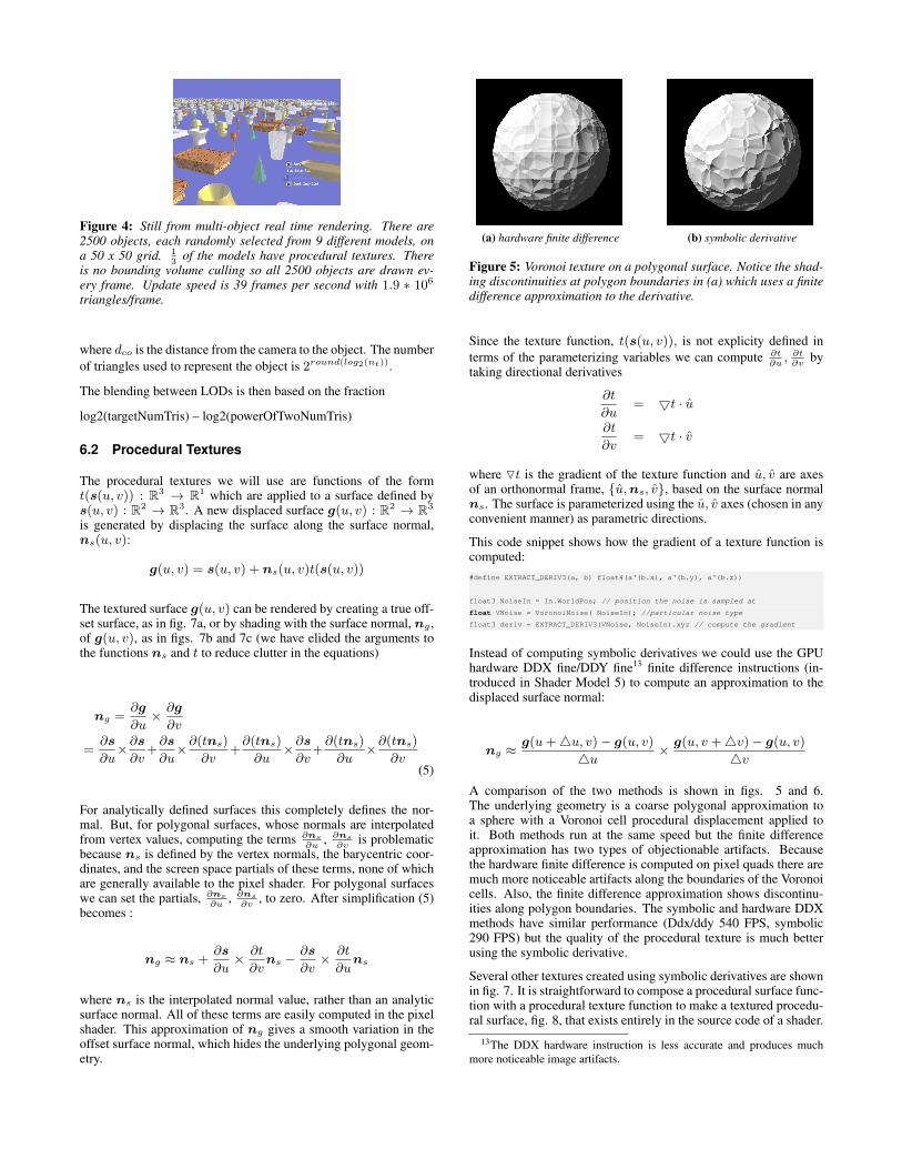
Figure 4: Still from multi-object real time rendering. There are2500 objects, each randomly selected from 9 different models, ona 50 x 50 grid. 1

3of the models have procedural textures. There

is no bounding volume culling so all 2500 objects are drawn ev-ery frame. Update speed is 39 frames per second with 1.9 ∗ 106

triangles/frame.

where dco is the distance from the camera to the object. The numberof triangles used to represent the object is 2round(log2(nt)).

The blending between LODs is then based on the fraction

log2(targetNumTris) – log2(powerOfTwoNumTris)

6.2 Procedural Textures

The procedural textures we will use are functions of the formt(s(u, v)) : R3 → R1 which are applied to a surface defined bys(u, v) : R2 → R3. A new displaced surface g(u, v) : R2 → R3

is generated by displacing the surface along the surface normal,ns(u, v):

g(u, v) = s(u, v) + ns(u, v)t(s(u, v))

The textured surface g(u, v) can be rendered by creating a true off-set surface, as in fig. 7a, or by shading with the surface normal, ng ,of g(u, v), as in figs. 7b and 7c (we have elided the arguments tothe functions ns and t to reduce clutter in the equations)

ng =∂g

∂u× ∂g

∂v

=∂s

∂u×∂s∂v

+∂s

∂u×∂(tns)

∂v+∂(tns)

∂u×∂s∂v

+∂(tns)

∂u×∂(tns)

∂v(5)

For analytically defined surfaces this completely defines the nor-mal. But, for polygonal surfaces, whose normals are interpolatedfrom vertex values, computing the terms ∂ns

∂u, ∂ns

∂vis problematic

because ns is defined by the vertex normals, the barycentric coor-dinates, and the screen space partials of these terms, none of whichare generally available to the pixel shader. For polygonal surfaceswe can set the partials, ∂ns

∂u, ∂ns

∂v, to zero. After simplification (5)

becomes :

ng ≈ ns +∂s

∂u× ∂t

∂vns −

∂s

∂v× ∂t

∂uns

where ns is the interpolated normal value, rather than an analyticsurface normal. All of these terms are easily computed in the pixelshader. This approximation of ng gives a smooth variation in theoffset surface normal, which hides the underlying polygonal geom-etry.

(a) hardware finite difference (b) symbolic derivative

Figure 5: Voronoi texture on a polygonal surface. Notice the shad-ing discontinuities at polygon boundaries in (a) which uses a finitedifference approximation to the derivative.

Since the texture function, t(s(u, v)), is not explicity defined interms of the parameterizing variables we can compute ∂t

∂u, ∂t∂v

bytaking directional derivatives

∂t

∂u= 5t · u

∂t

∂v= 5t · v

where Ot is the gradient of the texture function and u, v are axesof an orthonormal frame, {u,ns, v}, based on the surface normalns. The surface is parameterized using the u, v axes (chosen in anyconvenient manner) as parametric directions.

This code snippet shows how the gradient of a texture function iscomputed:#define EXTRACT_DERIV3(a, b) float4(a‘(b.x), a‘(b.y), a‘(b.z))

float3 NoiseIn = In.WorldPos; // position the noise is sampled at

float VNoise = VoronoiNoise( NoiseIn); //particular noise type

float3 deriv = EXTRACT_DERIV3(VNoise, NoiseIn).xyz // compute the gradient

Instead of computing symbolic derivatives we could use the GPUhardware DDX fine/DDY fine13 finite difference instructions (in-troduced in Shader Model 5) to compute an approximation to thedisplaced surface normal:

ng ≈g(u+4u, v)− g(u, v)

4u × g(u, v +4v)− g(u, v)

4v

A comparison of the two methods is shown in figs. 5 and 6.The underlying geometry is a coarse polygonal approximation toa sphere with a Voronoi cell procedural displacement applied toit. Both methods run at the same speed but the finite differenceapproximation has two types of objectionable artifacts. Becausethe hardware finite difference is computed on pixel quads there aremuch more noticeable artifacts along the boundaries of the Voronoicells. Also, the finite difference approximation shows discontinu-ities along polygon boundaries. The symbolic and hardware DDXmethods have similar performance (Ddx/ddy 540 FPS, symbolic290 FPS) but the quality of the procedural texture is much betterusing the symbolic derivative.

Several other textures created using symbolic derivatives are shownin fig. 7. It is straightforward to compose a procedural surface func-tion with a procedural texture function to make a textured procedu-ral surface, fig. 8, that exists entirely in the source code of a shader.

13The DDX hardware instruction is less accurate and produces muchmore noticeable image artifacts.

(a) hardware finite difference (b) symbolic derivative

Figure 6: Close up of Voronoi texture. The finite difference approx-imation introduces jagged edges along Voronoi cell boundaries

For simplicity we did not implement antialiasing for the proceduraltextures, but it would be straightforward to compute the Jacobianrelating texture and screen space and use this to control the numberof octaves of procedural noise used to generate the texture.

Antialiasing procedural textures applied to procedural surfaces re-quires computing the mapping from texture space to screen space.These volume textures are not parameterized by the procedural sur-face parameterizing variables u, v so we must reparameterize thesurface to be consistent with the procedural textures. Because thetexture functions are roughly isotropic any orthonormal parametriz-ing basis for the surface will do. We have already derived such abasis, u, v. The differential mapping from the procedural surface toscreen space is then given by

∆x = DprojDs∆u

where

Dproj =

[∂x∂xw

∂x∂yw

∂x∂zw

∂y∂xw

∂y∂yw

∂y∂zw

]is the derivative of the world to screen space projection matrix, eas-ily computed using symbolic differentiation.

The vector [xw, yw, zw]T is the position of a point on the procedu-ral surface, in world space. For polygonal surfaces the matrix Ds

is formed from the orthornormal surface basis:

Ds = [u, v]

The surface to screen mapping matrix

Dscr = DprojDs

is 2 by 2. The stretching, or shrinking, of the texture on the screencan be approximated by computing the SVD of this matrix. We useJacobi iteration, which for 2 by 2 matrices is guaranteed to con-verge to a solution in a single iteration. It is also numerically wellconditioned and relatively efficient14. One could also directly solvethe characteristic equation

Det[DT

scrDscr − λI]

= 0

Det

[a11 − λi a12a21 a22 − λi

]= 0

which gives a quadratic equation in λi

14The code for Jacobi iteration is included in the supplementary materials.

(a) Displacement surface (b) Fractal Voronoi (c) Lava Planet

Figure 7: Other procedural textures generated using symbolicderivatives. (a) is a true displacement surface. (b), (c) are bothnormal mapped.

𝑓: 𝑅2 ⇒ 𝑅3 𝑓: 𝑅1 ⇒ 𝑅2 𝑓: 𝑅1 ⇒ 𝑅2

Profile curve Cross-section curve Surface

+

𝑓: 𝑅3 ⇒ 𝑅1

Fractal Voronoi texture

=

Figure 8: Fractal Voronoi texture applied to procedurally gener-ated surface

(a11 − λi)(a22 − λi)− a21a12 = 0

This will take slightly less computation but squares the conditionnumber of Dscr . For typical graphics purposes this probably hasacceptable numerical properties.

Singular values less than 1 represent a shrinking of the texture,and consequently an increase in spatial frequencies present on thescreen. Values greater than 1 represent a stretching of the texture.We find the minimum singular value and use this to compute a scalefactor α which is applied to the texture normal offset equation

g(u, v) = s(u, v) + αns(u, v)t(s(u, v))

for true displacement surfaces or

ng = ns + α

(t∂ns

∂u+ ns

∂t

∂u

)×(t∂ns

∂v+ ns

∂t

∂v

)for normal mapped surfaces.

7 Results and Discussion

All timings reported in this section were performed on an Intel(R)Xeon(R) CPU E5640 @ 2.67GHz, 4 Cores with an ATI Radeon HD5870 GPU, 1024MB GDDR5, core clock 850MHz, memory clock1200MHz .

The procedural surfaces render at high rates, measured in trian-gles/sec., especially at high triangulation counts. Table 1 shows thetriangle rendering rates for a procedural lamp object. The renderingcomputes diffuse lighting, with the lamp object filling a 640x480

Triangles Tri/sec.200*103 540*106

20*103 333*106

2*103 50*106

576 19.2*106

Table 1: Rendering speed of procedurally defined lamp object atvarious triangulation levels. Triangle rendering speeds do not in-clude the time required to run the render loop setup which consistsof: screen clear, control and text display.

Object Only surface Surface + normal increasecomputations computations

sphere 36 47 17%lamp 79 96 30%

doric column 1454 2221 54%

Table 2: Computation required by the symbolic differentiation tocompute the exact surface normal. The doric column has the largestincrease because of the large number of computations required tocompute the procedural texture offset.

window, using the symbolic derivative to compute the normal atevery pixel.

The overhead associated with calling the shaders for the proceduralsurfaces (each object is one shader call) doesn’t become extremeuntil the number of objects is quite large. Fig. 4 shows a still froman animation with 2500 procedural objects, 1

3of which have proce-

dural textures. We did not implement bounding volume culling, anobvious efficiency improvement, so all 2500 objects are drawn eachframe. Even with this large number of objects the update rate was39 frames per second with 1.9∗106 triangles per frame, or 73∗106

triangles/sec. For a scene with a 100 object grid (not illustrated)the update rate at 3,300,000 tris/frame was 43Hz, or 142 milliontris/second.

In general the cost of computing derivatives is quite small. In Table2 we show the incremental cost of computing the exact symbolicsurface normal for three different procedural surfaces. The largestincrease is only about 50%, which occurs only for the doric columnobject. This object has a very complex procedural texture, which iscounted in the normal computations but not in the surface compu-tations.

Overall the system performs as we had hoped: derivatives are easyto specify and the resulting derivative code is very efficient. How-ever, there is one thing we hope to change in future versions. Whenwe designed the system the assumption was that derivative assign-ment would be uncommon, so the interaction between derivativeassignment and taking derivatives through functions would not beburdensome to the programmer. In real world shaders we discov-ered that the functions floor, ceil, frac, which do not havedefault derivative rules, occurred much more frequently than wesupposed. Derivative assignment had to be used in many shaders,which required all those shaders to have an additional derivativevariable argument. In future versions we hope to provide defaultderivative definitions for floor, ceil, frac which will elimi-nate this problem if no other derivative assignments are used. Wealso may ease the restriction on taking derivatives with respect tointerior nodes, which would allow derivative assignment to be usedinside functions without requiring an extra derivative variable.

8 Conclusion and Future Work

The new symbolic differentiation language feature now makes itpossible to easily and efficiently compute derivatives of complexfunctions in GPU shaders. The derivatives are generally quite effi-cient; in the example applications the symbolic derivative capabilityimproved the quality of texture rendering, with no loss in speed rel-ative to hardware finite differencing, and allowed for the renderingof procedural surfaces at very high speed. Many other applicationswill also benefit from this new feature.

In the future we may add variable dependency tracking, whichshould eliminate the need to pass differentiation variables betweenfunctions. We may also implement the full D* algorithm [Guenter2007] if the domain dimension of typical functions increases sub-stantially.

References

BISCHOF, C., ROH, L., AND MAUER-OATS, A. 1997. Adic: Anextensible automatic differentiation tool for ansi-c. Tech report27, 1427–1456.

GUENTER, B. 2007. Efficient symbolic differentiation algorithmfor graphics applications. ACM Computer Graphics 27, 3, 108.

HANRAHAN, P. 2009. Domain-specific languages for heteroge-nous gpu computing. NVIDIA Technology Conference.

SNYDER, J. 1992. Generative Modeling for Computer Graphicsand CAD. Academic Press.

UPSTILL, S. 1989. The Renderman Companion. Addison Wesley.