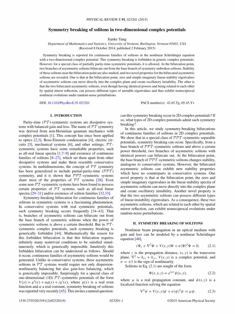
PHYSICAL REVIEW E 91, 023201 (2015)

Symmetry breaking of solitons in two-dimensional complex potentials

Jianke YangDepartment of Mathematics and Statistics, University of Vermont, Burlington, Vermont 05401, USA

(Received 8 October 2014; published 2 February 2015)

Symmetry breaking is reported for continuous families of solitons in the nonlinear Schrodinger equationwith a two-dimensional complex potential. This symmetry breaking is forbidden in generic complex potentials.However, for a special class of partially parity-time-symmetric potentials, it is allowed. At the bifurcation point,two branches of asymmetric solitons bifurcate out from the base branch of symmetry-unbroken solitons. Stabilityof these solitons near the bifurcation point are also studied, and two novel properties for the bifurcated asymmetricsolitons are revealed. One is that at the bifurcation point, zero and simple imaginary linear-stability eigenvaluesof asymmetric solitons can move directly into the complex plane and create oscillatory instability. The other isthat the two bifurcated asymmetric solitons, even though having identical powers and being related to each otherby spatial mirror reflection, can possess different types of unstable eigenvalues and thus exhibit nonreciprocalnonlinear evolutions under random-noise perturbations.

DOI: 10.1103/PhysRevE.91.023201 PACS number(s): 42.65.Tg, 05.45.Yv

I. INTRODUCTION

Parity-time (PT )-symmetric systems are dissipative sys-tems with balanced gain and loss. The name of PT symmetrywas derived from non-Hermitian quantum mechanics withcomplex potentials [1]. This concept has since been appliedto optics [2,3], Bose-Einstein condensation [4], electric cir-cuits [5], mechanical systems [6], and other settings. PT -symmetric systems have some remarkable properties, suchas all-real linear spectra [1,7–9] and existence of continuousfamilies of solitons [8–27], which set them apart from otherdissipative systems and make them resemble conservativesystems. In multidimensions, the concept of PT symmetryhas been generalized to include partial-parity-time (PPT )symmetry, and it is shown that PPT -symmetric systemsshare most of the properties of PT systems [28]. Evensome non-PT -symmetric systems have been found to possesscertain properties of PT systems, such as all-real linearspectra [29–31] and/or existence of soliton families [32,33].

Symmetry-breaking bifurcation for continuous families ofsolitons in symmetric systems is a fascinating phenomenon.In conservative systems with real symmetric potentials,such symmetry breaking occurs frequently [34–43]. Thatis, branches of asymmetric solitons can bifurcate out fromthe base branch of symmetric solitons when the power ofsymmetric solitons is above a certain threshold. But in PT -symmetric complex potentials, such symmetry breaking isgenerically forbidden [44]. Mathematically the reason forthis forbidden bifurcation is that this bifurcation requiresinfinitely many nontrivial conditions to be satisfied simul-taneously, which is generically impossible. Intuitively thisforbidden bifurcation can be understood as follows. Shouldit occur, continuous families of asymmetric solitons would begenerated. Unlike in conservative systems, these asymmetricsolitons in PT systems would require not only dispersion-nonlinearity balancing but also gain-loss balancing, whichis generically impossible. Surprisingly for a special class ofone-dimensional (1D) PT -symmetric potentials of the formV (x) = g2(x) + αg(x) + ig′(x), where g(x) is a real evenfunction and α a real constant, symmetry breaking of solitonswas reported very recently [45]. This invites a natural question:

can this symmetry breaking occur in 2D complex potentials? Ifso, what types of 2D complex potentials admit such symmetrybreaking?

In this article, we study symmetry-breaking bifurcationsof continuous families of solitons in 2D complex potentials.We show that in a special class of PPT -symmetric separablepotentials, symmetry breaking can occur. Specifically, from abase branch of PPT -symmetric solitons and above a certainpower threshold, two branches of asymmetric solitons withidentical powers can bifurcate out. At the bifurcation point,the base branch of PPT -symmetric solitons changes stability,analogous to conservative systems. However, the bifurcatedasymmetric solitons can exhibit new stability propertieswhich have no counterparts in conservative systems. Onenovel property is that at the bifurcation point, the zero andsimple imaginary eigenvalues in the linear-stability spectra ofasymmetric solitons can move directly into the complex planeand create oscillatory instability. Another novel property isthat the two asymmetric solitons can possess different typesof linear-instability eigenvalues. As a consequence, these twoasymmetric solitons, which are related to each other by spatialmirror reflection, can exhibit nonreciprocal evolutions underrandom-noise perturbations.

II. SYMMETRY BREAKING OF SOLITONS

Nonlinear beam propagation in an optical medium withgain and loss can be modeled by a nonlinear Schrodingerequation [46],

i�z + ∇2� + V (x,y)� + σ |�|2� = 0, (2.1)

where z is the propagation distance, (x,y) is the transverseplane, ∇2 = ∂xx + ∂yy , V (x,y) is a complex potential, andσ = ±1 is the sign of nonlinearity.

Solitons in Eq. (2.1) are sought of the form

�(x,y,z) = eiμzψ(x,y), (2.2)

where μ is a real propagation constant, and ψ(x,y) is alocalized function solving the equation

∇2ψ + V (x,y)ψ + σ |ψ |2ψ = μψ. (2.3)

1539-3755/2015/91(2)/023201(9) 023201-1 ©2015 American Physical Society

JIANKE YANG PHYSICAL REVIEW E 91, 023201 (2015)

If the complex potential V (x,y) is PT symmetric orPPT symmetric, continuous families of PT -symmetric orPPT -symmetric solitons are admitted [18,28], but symmetrybreaking of such solitons is generically forbidden [44].However, for certain special forms of 1D PT potentials,symmetry breaking of 1D solitons has been reported veryrecently [45].

In this article, we show that symmetry breaking of 2Dsolitons is also possible in the model (2.1) for a special classof complex potentials,

V (x,y) = g2(x) + αg(x) + ig′(x) + h(y), (2.4)

where g(x) is a real even function, i.e.,

g(−x) = g(x),

h(y) is an arbitrary real function, and α is a real constant.This potential is separable in (x,y), and its imaginary part isy independent. In addition, this potential is PPT symmetric,i.e.,

V ∗(x,y) = V (−x,y), (2.5)

where the asterisk represents complex conjugation. Due toseparability of this potential, it is easy to see that its linearspectrum can be all real [28]. Note that a potential of the formin Eq. (2.4) but with x and y switched is equivalent to Eq. (2.4)and thus does not deserve separate consideration.

The x component of the separable potential (2.4) is the sameas the 1D complex potential for symmetry breaking as reportedin Ref. [45], but the y component of this separable potential isreal and quite different. Should this y component be complexand also take the form of its x component, we have found thatsymmetry breaking would no longer occur. This indicates thatsymmetry breaking in the special 2D potential (2.4) is by nomeans obvious and cannot be anticipated from the 1D potentialfor symmetry breaking in Ref. [45].

Below we use two explicit examples of the potential (2.4)to demonstrate symmetry breaking of 2D solitons and revealtheir unique linear-stability properties.

Example 1. In our first example, we take the potential (2.4)with

g(x) = 0.3[e−(x+1.2)2 + e−(x−1.2)2]

, (2.6)

α = 10, h(y) = 0. (2.7)

This is a y-independent stripe potential which is illustratedin Fig. 1. The spectrum of this potential is all real, and alleigenvalues lie in the continuous spectrum of (−∞,2.0569].

Solitons in Eq. (2.3) under this potential will be computedby the Newton-conjugate-gradient method. This method fea-tures high accuracy as well as fast speed. The application of thismethod for solitons in conservative systems has been describedin Refs. [47,48]. In those cases, the linear Newton-correctionequation was self-adjoint and thus could be solved directlyby preconditioned conjugate gradient iterations. However, thepresent Eq. (2.3) is dissipative; hence the resulting Newton-correction equation is non-self-adjoint. In this case, directconjugate gradient iterations on this equation would fail, andit is necessary to turn this equation into a normal equation andthen solve it by preconditioned conjugate gradient iterations.

x

y

(a)

−7 0 7−7

0

7

0

1

2

3

x

y

(b)

−7 0 7−7

0

7

−0.2

0

0.2

FIG. 1. (Color online) A stripe complex potential (2.4) withEqs. (2.6) and (2.7) in Example 1. (a) Re(V ); (b) Im(V ).

In the Appendix, this Newton-conjugate-gradient method forEq. (2.3) is explained in more detail.

Using this Newton-conjugate-gradient method, we find thatfrom the edge of the continuous spectrum μ0 = 2.0569, acontinuous family of solitons ψs(x,y; μ), localized in both x

and y directions, bifurcates out. The power curve of this solitonfamily is displayed in Fig. 2 (blue curve in the first row). Herethe power is defined as

P (μ) =∫ ∞

−∞

∫ ∞

−∞|ψ(x,y; μ)|2dxdy.

At two points, a and b, of this power curve, soliton profiles areshown in Fig. 2 (the second and third rows). These solitonsrespect the same PPT symmetry of the potential, i.e.,

ψ∗s (x,y) = ψs(−x,y). (2.8)

The existence of this soliton family respecting the samesymmetry of the potential is anticipated.

What is surprising is that, when the power of this solitonfamily reaches a critical value Pc ≈ 8.60, two branchesof asymmetric solitons bifurcate out through a pitchforkbifurcation. These asymmetric solitons do not respect thePPT symmetry (2.8). At the same μ value, they haveidentical powers and are related to each other through a spatialreflection:

ψ (1)∗a (x,y) = ψ (2)

a (−x,y). (2.9)

The power curve of these two branches of asymmetric solitonsis plotted in Fig. 2 (red curve in the first row). Notice thatunlike the symmetric (base) branch, the power slope of theseasymmetric branches is negative at the bifurcation point. Atpoint c of the asymmetric branches, the profile for one of thetwo asymmetric solitons is displayed in Fig. 2 (the bottomrow). Asymmetry in its profile can clearly be seen. Thesesolitons have lost the PPT symmetry of the underlyingpotential; thus symmetry breaking has occurred.

Next we analyze linear stability of these symmetric andasymmetric solitons. To determine linear stability, we perturbthese solitons as

�(x,y,z) = eiμz[ψ(x,y) + u(x,y) eλz + w∗(x,y) eλ∗z],

where |u|,|w| � |ψ |. After substitution into Eq. (2.1) andlinearizing, we arrive at the eigenvalue problem

L(

u

w

)= λ

(u

w

), (2.10)

023201-2

SYMMETRY BREAKING OF SOLITONS IN TWO- . . . PHYSICAL REVIEW E 91, 023201 (2015)

2 2.5 30

5

10

15

μ

P

2.3 2.4

8

9

10

μ

P

a

b

c

x

y

|ψ| at “a”

−7 0 7−7

0

7

0

0.6

1.2

x

y

phase of ψ at “a”

−7 0 7−7

0

7

−0.1

0

0.1

x

y

|ψ| at “b”

−7 0 7−7

0

7

0

0.6

1.2

x

y

phase of ψ at “b”

−7 0 7−7

0

7

−0.1

0

0.1

x

y

|ψ| at “c”

−7 0 7−7

0

7

0

0.6

1.2

x

y

phase of ψ at “c”

−7 0 7−7

0

7

−0.1

0

0.1

FIG. 2. (Color online) Symmetry breaking of solitons in Exam-ple 1. First row: Power curves of symmetric (blue) and asymmetric(red) solitons; the right panel is an amplification of the left panelaround the bifurcation point. Second to fourth rows: Soliton profilesat points a, b, and c of the power curve. Left panels: Amplitude fields.Right panels: Phase fields.

where

L = i

(L11 L12

L21 L22

)

and

L11 = ∇2 + V − μ + 2σ |ψ |2,L12 = σψ2, L21 = −σ (ψ2)∗,

L22 = −(∇2 + V − μ + 2σ |ψ |2)∗.

If eigenvalues with positive real parts exist, the soliton islinearly unstable; otherwise it is linearly stable.

Linear-stability eigenvalues exhibit important differencesfor symmetric and asymmetric solitons. For symmetric soli-tons ψs(x,y), it is easy to show from soliton symmetry (2.8)and potential symmetry (2.5) that, if {λ, u(x,y), w(x,y)}

is an eigenmode, then so are {λ∗, w∗(x,y), u∗(x,y)},{−λ, w(−x,y), u(−x,y)}, and {−λ∗, u∗(−x,y), w∗(−x,y)}.Thus for symmetric solitons, real and imaginary eigenvaluesappear as pairs (λ, − λ), and complex eigenvalues appear asquartets {λ,λ∗, − λ, − λ∗}.

For asymmetric solitons, however, the situation is different.While it is still true that if λ is an eigenvalue, so is λ∗, butdue to the lack of soliton symmetry (2.8), −λ and −λ∗ are nolonger eigenvalues. In other words, for asymmetric solitons,complex eigenvalues appear as conjugate pairs (λ,λ∗), not asquartets, and real eigenvalues appear as single eigenvalues,not as (λ, − λ) pairs. These differences on eigenvalue sym-metry between symmetric and asymmetric solitons will haveimportant implications, as we will see later in this section.

For the two branches of asymmetric solitons, their linear-stability eigenvalues are related. Indeed, from the mirror sym-metry (2.9) between these two bifurcated soliton branches, it iseasy to see that if λ is an eigenvalue of the soliton ψ (1)

a (x,y; μ),then −λ∗ will be an eigenvalue of the companion solitonψ (2)

a (x,y; μ). In other words, the linear-stability spectrum ofthe soliton ψ (1)

a (x,y; μ) is a mirror reflection of that spectrumof the companion soliton ψ (2)

a (x,y; μ) around the imaginaryaxis.

The eigenvalue problem (2.10) can be computed by theFourier collocation method (for the full spectrum) or theNewton-conjugate-gradient method (for individual discreteeigenvalues) [48]. We find that near the symmetry-breakingbifurcation point μc ≈ 2.33, symmetric solitons are stablebefore the bifurcation point (μ < μc) and unstable after it(μ > μc), and both branches of asymmetric solitons areunstable. This stability behavior is marked on the power curvein Fig. 3 (upper left panel). To shed light on the origins ofthese stabilities and instabilities, linear-stability spectra atthree points, a–c, of this power curve, for the three solitonsdisplayed in Fig. 2, are displayed in panels Figs. 3(a)–3(c),

2.3 2.4

8

9

10

μ

P

a

b

c

−0.5 0 0.5−0.5

0

0.5

Re(λ)

Im(λ

)

(a)

−0.5 0 0.5−0.5

0

0.5

Re(λ)

Im(λ

)

(b)

−0.5 0 0.5−0.5

0

0.5

Re(λ)

Im(λ

)

(c)

FIG. 3. (Color online) Linear-stability behaviors of solitons nearthe symmetry-breaking point in Example 1. Upper left panel: Thepower curve with stability marked (solid blue for stable and dashedred for unstable). (a–c) Linear-stability spectra for the solitons atpoints a, b, and c of the power curve.

023201-3

JIANKE YANG PHYSICAL REVIEW E 91, 023201 (2015)

respectively. We see from Fig. 3(a) that before the bifurcation,the symmetric soliton has a pair of discrete eigenvalues on theimaginary axis. At the bifurcation point, this pair of imaginaryeigenvalues coalesce at the origin. After bifurcation, thesecoalesced eigenvalues split along the real axis in oppositedirections for both symmetric and asymmetric solitons. Alongthe symmetric branch, the two split eigenvalues form a (λ, − λ)pair [see Fig. 3(b)]. But along the asymmetric branches, thetwo split eigenvalues do not form a (λ, − λ) pair since theyhave different magnitudes [see Fig. 3(c)]. These spectra showthat the instability of symmetric and asymmetric solitons afterbifurcation is due to the zero-eigenvalue splitting along thereal axis at μ = μc, and this instability is exponential (causedby real eigenvalues).

It is interesting to observe that the power-curve structure andthe associated stability behaviors in Fig. 3 (upper left panel)resemble those in the conservative generalized nonlinearSchrodinger equations with real potentials (see Fig. 2(c) inRef. [43]). In that conservative case, it was shown that if thepower slopes of the symmetric and asymmetric solitons at thebifurcation point have opposite signs, then both solitons willshare the same stability or instability [43]. Figure 3 of thepresent article suggests that such a statement might hold forcomplex potentials as well.

The linear-stability results of Fig. 3 are corroboratedby nonlinear evolution simulations of those solitons underrandom-noise perturbations. To demonstrate, we perturb thethree solitons of Fig. 2 by 1% random-noise perturbations,and their nonlinear evolutions are displayed in Fig. 4. As canbe seen, the perturbed symmetric soliton before bifurcationshows little change even after z = 100 units of propagation,confirming that it is linearly stable (see top row of Fig. 4). Theperturbed symmetric soliton after bifurcation, on the otherhand, clearly breaks up and evolves into a highly asymmetricprofile after 20 units of propagation, confirming that it islinearly unstable (see middle row of Fig. 4). The perturbedasymmetric soliton, whose initial intensity hump is locatedat the right side, also breaks up and evolves into a profilewhose intensity hump moves to the left side after 50 units ofpropagation, confirming that it is linearly unstable as well (seebottom row of Fig. 4).

Example 2. In our second example, we take the poten-tial (2.4) with

g(x) = 0.3[e−(x+1.2)2 + e−(x−1.2)2]

, α = 10,

and

h(y) = 2[e−(y+1.2)2 + 0.8e−(y−1.2)2]

.

This potential is illustrated in Fig. 5. Its real part is no longer astripe potential, nor is it symmetric in y. The spectrum of thispotential is all-real, and it consists of three discrete eigenvaluesof {2.5643,2.5689,3.2028} and the continuous spectrum of(−∞,2.0569].

From the largest discrete eigenvalue of μ0 = 3.2028, acontinuous family of PPT -symmetric solitons bifurcatesout. The power curve of this soliton family is plotted inFig. 6(A) (blue curve). When the power of these solitonsreaches a threshold of Pc ≈ 5.24 (at μc ≈ 3.56), two branches

x

y

z = 0(a)

−7 0 7−7

0

7

0

0.6

1.2

x

y

z = 100

−7 0 7−7

0

7

0

0.6

1.2

x

y

z = 0(b)

−7 0 7−7

0

7

0

0.6

1.2

x

y

z = 20

−7 0 7−7

0

7

0

1

2

x

y

z = 0(c)

−7 0 7−7

0

7

0

0.6

1.2

x

y

z = 50

−7 0 7−7

0

7

0

0.6

1.2

FIG. 4. (Color online) Nonlinear evolutions of the three solitonsin Fig. 2 under 1% random-noise perturbations (locations of thesesolitons on the power curve are marked in both Figs. 2 and 3).

of asymmetric solitons bifurcate out, whose power curves arealso displayed in Fig. 6(A) (red curve). As before, these twoasymmetric solitons are related to each other by Eq. (2.9); thusthey have identical powers. Enlargement of this power curvenear the bifurcation point is shown in Fig. 6(B). At pointsa–d of this amplified power diagram, the solitons’ amplitudeprofiles are plotted in Fig. 6 (middle and bottom rows). Herepoints c and d are the same power points but on differentasymmetric-soliton branches. We can see that solitons at pointsa and b of the base branch are PPT symmetric, with point abefore bifurcation and point b after it. The solitons at pointsc and d of the bifurcated branches, however, are asymmetric,with the energy concentrated on the right and left sides ofthe x axis, respectively. In this example, power slopes of the

x

y

(a)

−6 0 6−6

0

6

0

2

4

x

y

(b)

−6 0 6−6

0

6

−0.2

0

0.2

FIG. 5. (Color online) The PPT -symmetric complex poten-tial (2.4) in Example 2. (a) Re(V ); (b) Im(V ).

023201-4

SYMMETRY BREAKING OF SOLITONS IN TWO- . . . PHYSICAL REVIEW E 91, 023201 (2015)

3.2 3.6 40

5

10

μ

P

(A)

3.5 3.6 3.7

4

5

6

μ

P

(B)

a

b

c,d

x

y

|ψ| at “a”

−6 0 6−6

0

6

0

0.6

1.2

x

y

|ψ| at “b”

−6 0 6−6

0

6

0

0.6

1.2

x

y

|ψ| at “c”

−6 0 6−6

0

6

0

0.6

1.2

x

y

|ψ| at “d”

−6 0 6−6

0

6

0

0.6

1.2

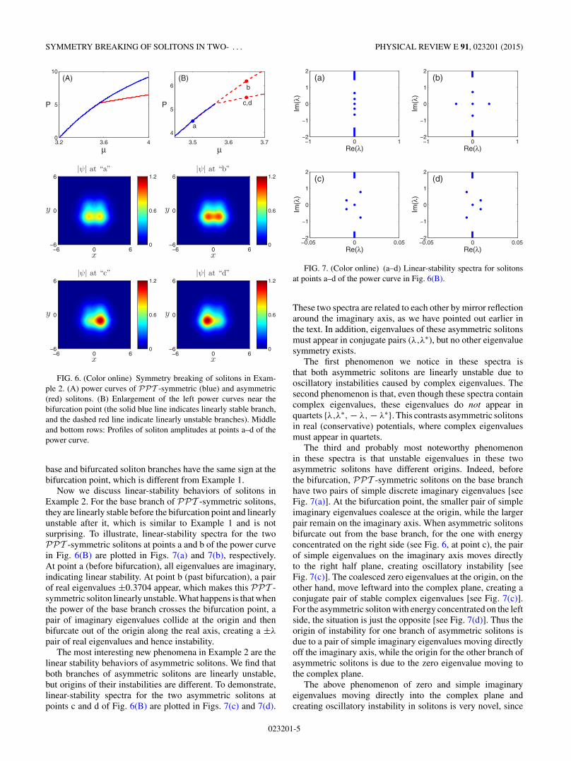
FIG. 6. (Color online) Symmetry breaking of solitons in Exam-ple 2. (A) power curves of PPT -symmetric (blue) and asymmetric(red) solitons. (B) Enlargement of the left power curves near thebifurcation point (the solid blue line indicates linearly stable branch,and the dashed red line indicate linearly unstable branches). Middleand bottom rows: Profiles of soliton amplitudes at points a–d of thepower curve.

base and bifurcated soliton branches have the same sign at thebifurcation point, which is different from Example 1.

Now we discuss linear-stability behaviors of solitons inExample 2. For the base branch of PPT -symmetric solitons,they are linearly stable before the bifurcation point and linearlyunstable after it, which is similar to Example 1 and is notsurprising. To illustrate, linear-stability spectra for the twoPPT -symmetric solitons at points a and b of the power curvein Fig. 6(B) are plotted in Figs. 7(a) and 7(b), respectively.At point a (before bifurcation), all eigenvalues are imaginary,indicating linear stability. At point b (past bifurcation), a pairof real eigenvalues ±0.3704 appear, which makes this PPT -symmetric soliton linearly unstable. What happens is that whenthe power of the base branch crosses the bifurcation point, apair of imaginary eigenvalues collide at the origin and thenbifurcate out of the origin along the real axis, creating a ±λ

pair of real eigenvalues and hence instability.The most interesting new phenomena in Example 2 are the

linear stability behaviors of asymmetric solitons. We find thatboth branches of asymmetric solitons are linearly unstable,but origins of their instabilities are different. To demonstrate,linear-stability spectra for the two asymmetric solitons atpoints c and d of Fig. 6(B) are plotted in Figs. 7(c) and 7(d).

−1 0 1−2

−1

0

1

2

Re(λ)

Im(λ

)

(a)

−1 0 1−2

−1

0

1

2

Re(λ)

Im(λ

)

(b)

−0.05 0 0.05−2

−1

0

1

2

Re(λ)

Im(λ

)

(c)

−0.05 0 0.05−2

−1

0

1

2

Re(λ)

Im(λ

)

(d)

FIG. 7. (Color online) (a–d) Linear-stability spectra for solitonsat points a–d of the power curve in Fig. 6(B).

These two spectra are related to each other by mirror reflectionaround the imaginary axis, as we have pointed out earlier inthe text. In addition, eigenvalues of these asymmetric solitonsmust appear in conjugate pairs (λ,λ∗), but no other eigenvaluesymmetry exists.

The first phenomenon we notice in these spectra isthat both asymmetric solitons are linearly unstable due tooscillatory instabilities caused by complex eigenvalues. Thesecond phenomenon is that, even though these spectra containcomplex eigenvalues, these eigenvalues do not appear inquartets {λ,λ∗, − λ, − λ∗}. This contrasts asymmetric solitonsin real (conservative) potentials, where complex eigenvaluesmust appear in quartets.

The third and probably most noteworthy phenomenonin these spectra is that unstable eigenvalues in these twoasymmetric solitons have different origins. Indeed, beforethe bifurcation, PPT -symmetric solitons on the base branchhave two pairs of simple discrete imaginary eigenvalues [seeFig. 7(a)]. At the bifurcation point, the smaller pair of simpleimaginary eigenvalues coalesce at the origin, while the largerpair remain on the imaginary axis. When asymmetric solitonsbifurcate out from the base branch, for the one with energyconcentrated on the right side (see Fig. 6, at point c), the pairof simple eigenvalues on the imaginary axis moves directlyto the right half plane, creating oscillatory instability [seeFig. 7(c)]. The coalesced zero eigenvalues at the origin, on theother hand, move leftward into the complex plane, creating aconjugate pair of stable complex eigenvalues [see Fig. 7(c)].For the asymmetric soliton with energy concentrated on the leftside, the situation is just the opposite [see Fig. 7(d)]. Thus theorigin of instability for one branch of asymmetric solitons isdue to a pair of simple imaginary eigenvalues moving directlyoff the imaginary axis, while the origin for the other branch ofasymmetric solitons is due to the zero eigenvalue moving tothe complex plane.

The above phenomenon of zero and simple imaginaryeigenvalues moving directly into the complex plane andcreating oscillatory instability in solitons is very novel, since

023201-5

JIANKE YANG PHYSICAL REVIEW E 91, 023201 (2015)

it contrasts conservative systems with real potentials. In realpotentials, linear-stability complex eigenvalues of solitonsappear as quartets {λ,λ∗, − λ, − λ∗}. Partly because of it,bifurcation of complex eigenvalues off the imaginary axistypically occurs through collision of imaginary eigenvaluesof opposite Krein signatures (a bifurcation referred to asHamiltonian-Hopf bifurcation in the literature [49]). In addi-tion, complex eigenvalues (not on the real and imaginary axes)cannot bifurcate from the origin when two simple eigenvaluescollide there. But in complex potentials, the situation can bevery different as is explained above.

The fourth phenomenon in the spectra of Fig. 7 isthat, the maximal growth rates of perturbations in thesetwo asymmetric solitons are different. Indeed the unstableeigenvalues in Fig. 7(c) are 0.0067 ± 0.7721i, giving a growthrate of 0.0067; while the unstable eigenvalues in Fig. 7(d)are 0.0090 ± 0.2692i, giving a larger growth rate of 0.0090.The fifth phenomenon is that these oscillatory instabilities inasymmetric solitons are rather weak due to these small growthrates. This means that these oscillatory instabilities will takelong distances to develop.

Of the five phenomena mentioned above, the third andfourth ones are the most fundamental, and they are rarelyseen (if ever) for asymmetric solitons arising from symmetry-breaking bifurcations.

Since the two branches of asymmetric solitons havedifferent origins of instability and different growth rates, smallperturbations in these solitons will grow differently, leadingto nonreciprocal developments of instability. To demonstrate,evolutions of the two asymmetric solitons in Fig. 6 under 1%random-noise perturbations are displayed in Fig. 8. We seethat even though these two asymmetric solitons are relatedto each other by a mirror reflection (2.9) and are reciprocal,their evolutions under weak perturbations are not reciprocal.Indeed, after 1000 distance units of propagation, they reachsimilar asymmetric states. This nonreciprocal evolution is mostvisible in Figs. 8(c) and 8(d), where amplitude evolutions atspatial positions (x,y) = (−1.2, − 1.2) and (1.2, − 1.2) forthe two perturbed asymmetric solitons are plotted respectively.These amplitude evolutions vividly confirm that (a) the twoasymmetric solitons are linearly unstable, (b) their instabilitiesare caused by different unstable modes with different growthrates, and (c) the nonlinear evolutions are nonreciprocal eventhough the asymmetric solitons are.

In Example 2, when asymmetric solitons bifurcate out,the coalesced zero eigenvalue and the pair of imaginaryeigenvalues move in opposite directions in the complexplane, causing instability to both asymmetric solitons [seeFigs. 7(c) and 7(d)]. For other potentials and/or nonlinearities,if those eigenvalues bifurcate in the same direction, then oneasymmetric soliton would be linearly stable and the otherunstable. Such a scenario would be very remarkable. Whethersuch scenarios exist or not is an open question.

In the above two examples, symmetry breaking wasobserved for complex potentials of the form (2.4). We havealso tried a related class of complex potentials,

V (x,y) = g2(x) + αg(x) + ig′(x) + h2(y) + βh(y) + ih′(y),

(2.11)

x

y

z = 0(a)

−6 0 6−6

0

6

0

0.6

1.2

x

y

z = 1000

−6 0 6−6

0

6

0

0.6

1.2

x

y

z = 0(b)

−6 0 6−6

0

6

0

0.6

1.2

x

y

z = 1000

−6 0 6−6

0

6

0

0.6

1.2

0 200 400 600 800 10000.4

0.6

0.8

1

1.2

z

ampl

itude

s (c)

0 200 400 600 800 10000.4

0.6

0.8

1

1.2

z

ampl

itude

s (d)

FIG. 8. (Color online) Nonreciprocal evolutions of two recipro-cal asymmetric solitons in Fig. 6 under 1% random-noise pertur-bations in Example 2. First and second rows: Initially perturbedasymmetric solitons and their evolved solutions at z = 1000. (c,d)Evolutions of solution amplitudes |�| versus z at two spatial positions(x,y) = (−1.2, − 1.2) (blue) and (1.2, − 1.2) (red) for the twoasymmetric solitons of Fig. 6 under perturbations.

where g(x) and h(y) are real even functions, and α and β arereal constants. This potential isPT symmetric, i.e., V ∗(x,y) =V (−x, − y), and it admits PT -symmetric solitons. But wedid not find symmetry breaking here; i.e., we did not findbranches of asymmetric solitons bifurcating from the branchof PT -symmetric solitons.

Why does symmetry breaking occur in potentials of theform in Eq. (2.4) but not in some others such as Eq. (2.11)? Thisquestion is not clear yet. In fact, even for the one-dimensionalsymmetry-breaking bifurcations reported in Ref. [45], thereason for that symmetry breaking was not entirely cleareither. In the 1D case, the forms of potentials for symmetrybreaking in PT -symmetric potentials and for soliton familiesin asymmetric potentials are the same [32,45]. For thosepotentials, there is a conserved quantity which, when combinedwith a shooting argument, helps explain the existence ofsoliton families in asymmetric complex potentials [33]. Thatconserved quantity may prove useful to explain symmetrybreaking in those 1D potentials as well.

023201-6

SYMMETRY BREAKING OF SOLITONS IN TWO- . . . PHYSICAL REVIEW E 91, 023201 (2015)

For the present class of 2D potentials, Eq. (2.4), we havefound that Eq. (2.1) also admits a conservation law,

Qt + Jx + Ky = 0, (2.12)

where

Q = i�(�∗x − ig�∗),

J = ��∗yy + |�x + ig�|2 − i��∗

t

+(

h − α2

4

)|�|2 + σ

2|�|4,

K = �y(�∗x − ig�∗) − �(�∗

x − ig�∗)y,

and

g(x) = g(x) + α

2.

For solitons (2.2), substituting their functional form into theabove conservation law, a reduced conservation law for thesoliton function ψ(x,y) can also be derived. For the otherclass of potentials, Eq. (2.11), however, we could not findsuch a conservation law. This suggests that there is indeed aconnection between the existence of a conservation law and thepresence of symmetry breaking of solitons. But this connectionin the 2D case would be harder to establish since shooting-typearguments would break down.

In 1D, symmetry breaking in symmetric potentials andexistence of soliton families in asymmetric potentials occurin complex potentials of the same form [32,45]. This invites anatural question: for the class of 2D complex potentials (2.4)which admits symmetry breaking, if these potentials are notPPT symmetric, i.e., if g(x) is real but not even, can theysupport continuous families of solitons? The answer is positiveas our preliminary numerics have shown.

III. SUMMARY AND DISCUSSION

In this article, we reported symmetry breaking of solitonsin the nonlinear Schrodinger equation with a class of two-dimensional PPT -symmetric complex potentials (2.4). Atthe bifurcation point, two branches of asymmetric solitonsbifurcate out from the base branch of PPT -symmetricsolitons, and this bifurcation is quite surprising. Stability ofthese solitons near the bifurcation point was also studied. In thetwo examples we investigated, we found that the base branchof symmetric solitons changes stability at the bifurcationpoint, and the bifurcated asymmetric solitons are unstable.For the asymmetric solitons, two novel stability propertieswere further revealed. One is that, at the bifurcation point,the zero and simple imaginary linear-stability eigenvaluesof asymmetric solitons can move directly into the complexplane and create oscillatory instability. The other is thatthe two bifurcated asymmetric solitons, even though havingidentical powers and being related to each other by spatialmirror reflection, can have different origins of linear instabilityand thus exhibit nonreciprocal nonlinear evolutions underrandom-noise perturbations.

We should point out that the complex potentials (2.4)possess a single (PPT ) symmetry; thus they must be in that

special form in order for symmetry breaking to occur. If acomplex potential exhibits more than one spatial symmetry,say double PPT symmetries,

V ∗(x,y) = V (−x,y), V ∗(x,y) = V (x, − y),

or one PT and one PPT symmetry, say

V ∗(x,y) = V (−x, − y), V ∗(x,y) = V (−x,y),

then this potential can admit symmetry breaking withoutthe need for special functional forms (this prospect hasbeen mentioned in Ref. [44] and confirmed by our ownnumerics). When symmetry breaking occurs in such double-symmetry potentials, the base branch of solitons respects bothsymmetries of the potential, while the bifurcated solitons loseone symmetry but retain the other. The simple mathematicalreason for symmetry breakings in double-symmetry potentialsis that the infinitely many analytical conditions for symmetrybreaking in Ref. [44] are all satisfied automatically dueto the remaining symmetry of the bifurcated solitons. Thatsituation is fundamentally different from symmetry breakingsin potentials of special forms such as Eq. (2.4), whichadmit a single spatial symmetry. The mathematical reason forsymmetry breaking in single-symmetry potentials of specialfunctional forms such as Eq. (2.4) is still not clear.

ACKNOWLEDGMENTS

This work was supported in part by the Air Force Officeof Scientific Research (Grant No. USAF 9550-12-1-0244) andthe National Science Foundation (Grant No. DMS-1311730).

APPENDIX: NUMERICAL METHOD FOR COMPUTINGSOLITONS IN COMPLEX POTENTIALS

In this Appendix, we describe the Newton-conjugate-gradient method for computing solitons in Eq. (2.3) with acomplex potential.

The general idea of the Newton-conjugate-gradient methodis that, for a nonlinear real-valued vector equation,

L0(u) = 0, (A1)

its solution u is obtained by Newton iterations

un+1 = un + un, (A2)

where the updated amount un is computed from the linearNewton-correction equation

L1nun = −L0(un), (A3)

where L1n is the linearization operator L1 of Eq. (A1) evaluatedat the approximate solution un. If L1 is self-adjoint, thenEq. (A3) can be solved directly by preconditioned conjugate-gradient iterations [47,48,50]. But if L1 is non-self-adjoint, wefirst multiply it by the adjoint operator of L1 and turn it into anormal equation,

LA1nL1nun = −LA

1nL0(un), (A4)

which is then solved by preconditioned conjugate gradientiterations.

023201-7

JIANKE YANG PHYSICAL REVIEW E 91, 023201 (2015)

For Eq. (2.3), we first split the complex function ψ and thecomplex potential V into their real and imaginary parts:

ψ = ψ1 + iψ2, V = V1 + iV2.

Substituting these equations into Eq. (2.3), we obtain two realequations for (ψ1,ψ2):

∇2ψ1 + (V1 − μ)ψ1 − V2ψ2 + σ(ψ2

1 + ψ22

)ψ1 = 0,

∇2ψ2 + (V1 − μ)ψ2 + V2ψ1 + σ(ψ2

1 + ψ22

)ψ2 = 0.

These two real equations are the counterpart of Eq. (A1) forthe vector function u = [ψ1,ψ2]T , where the superscript T

represents the transpose of a vector. The linearization operatorof the above nonlinear equations is

L1 =[L11 L12

L21 L22

],

where

L11 = ∇2 + V1 − μ + σ(3ψ2

1 + ψ22

),

L12 = 2σψ1ψ2 − V2,

L21 = 2σψ1ψ2 + V2,

L22 = ∇2 + V1 − μ + σ(3ψ2

2 + ψ21

).

This linearization operator is non-self-adjoint; thus the Newtoncorrection is obtained from solving the normal equation (A4),where the adjoint operator of L1 is

LA1 = LT

1 =[L11 L21

L12 L22

].

For Eq. (2.3), the preconditioner in conjugate-gradientiterations for solving the normal equation (A4) is taken as

M = diag[(∇2 + c)2,(∇2 + c)2],

where c is a positive constant (which we take as c = 3 in ourcomputations).

While the above numerical algorithm is developed for realfunctions (ψ1,ψ2), during computer implementation, it is moretime-efficient to recombine (ψ1,ψ2) into a complex functionψ , so that the derivatives of (ψ1,ψ2) can be obtained simultane-ously from ψ by the fast Fourier transform. Correspondingly,linear operators L1 and LA

1 acting on real vector functions arecombined into scalar complex operations as well. Due to thisrecombination, the code also becomes more compact.

In the Supplemental Material of this article [51], a sampleMATLAB code is provided for the computation of an asymmetricsoliton in Example 1 at μ = 2.4 (see Fig. 2, at point c). Ona desktop PC (Dell Optiplex 990 with CPU speed 3.3 GHz),this code takes 192 conjugate-gradient iterations and under1.5 s to finish with solution accuracy below 10−12.

[1] C. M. Bender and S. Boettcher, Phys. Rev. Lett. 80, 5243 (1998).[2] A. Ruschhaupt, F. Delgado, and J. G. Muga, J. Phys. A 38, L171

(2005).[3] R. El-Ganainy, K. G. Makris, D. N. Christodoulides, and Z. H.

Musslimani, Opt. Lett. 32, 2632 (2007).[4] H. Cartarius and G. Wunner, Phys. Rev. A 86, 013612 (2012).[5] J. Schindler, A. Li, M. C. Zheng, F. M. Ellis, and T. Kottos,

Phys. Rev. A 84, 040101(R) (2011).[6] C. M. Bender, B. Berntson, D. Parker, and E. Samuel, Am. J.

Phys. 81, 173 (2013).[7] Z. Ahmed, Phys. Lett. A 282, 343 (2001).[8] Z. H. Musslimani, K. G. Makris, R. El-Ganainy, and D. N.

Christodoulides, Phys. Rev. Lett. 100, 030402 (2008).[9] D. A. Zezyulin and V. V. Konotop, Phys. Rev. A 85, 043840

(2012).[10] H. Wang and J. Wang, Opt. Express 19, 4030 (2011).[11] Z. Lu and Z. Zhang, Opt. Express 19, 11457 (2011).[12] S. Hu, X. Ma, D. Lu, Z. Yang, Y. Zheng, and W. Hu, Phys. Rev.

A 84, 043818 (2011).[13] F. K. Abdullaev, Y. V. Kartashov, V. V. Konotop, and D. A.

Zezyulin, Phys. Rev. A 83, 041805 (2011).[14] R. Driben and B. A. Malomed, Opt. Lett. 36, 4323 (2011).[15] K. Li and P. G. Kevrekidis, Phys. Rev. E 83, 066608 (2011).[16] X. Zhu, H. Wang, L. X. Zheng, H. Li, and Y. J. He, Opt. Lett.

36, 2680 (2011).[17] Y. He, X. Zhu, D. Mihalache, J. Liu, and Z. Chen, Phys. Rev. A

85, 013831 (2012).[18] S. Nixon, L. Ge, and J. Yang, Phys. Rev. A 85, 023822

(2012).[19] C. Li, H. Liu, and L. Dong, Opt. Express 20, 16823 (2012).

[20] N. V. Alexeeva, I. V. Barashenkov, A. A. Sukhorukov, andYu. S. Kivshar, Phys. Rev. A 85, 063837 (2012).

[21] F. C. Moreira, F. Kh. Abdullaev, V. V. Konotop, and A. V. Yulin,Phys. Rev. A 86, 053815 (2012).

[22] D. A. Zezyulin and V. V. Konotop, Phys. Rev. Lett. 108, 213906(2012).

[23] V. V. Konotop, D. E. Pelinovsky, and D. A. Zezyulin, Europhys.Lett. 100, 56006 (2012).

[24] Y. V. Kartashov, Opt. Lett. 38, 2600 (2013).[25] I. V. Barashenkov, L. Baker, and N. V. Alexeeva, Phys. Rev. A

87, 033819 (2013).[26] P. G. Kevrekidis, D. E. Pelinovsky, and D. Y. Tyugin, SIAM J.

Appl. Dyn. Syst. 12, 1210 (2013).[27] D. A. Zezyulin and V. V. Konotop, J. Phys. A 46, 415301 (2013).[28] J. Yang, Opt. Lett. 39, 1133 (2014)[29] F. Cooper, A. Khare, and U. Sukhatme, Phys. Rep. 251, 267

(1995).[30] F. Cannata, G. Junker, and J. Trost, Phys. Lett. A 246, 219

(1998).[31] M.-A. Miri, M. Heinrich, and D. N. Christodoulides, Phys. Rev.

A 87, 043819 (2013).[32] E. N. Tsoy, I. M. Allayarov, and F. Kh. Abdullaev, Opt. Lett.

39, 4215 (2014).[33] V. V. Konotop and D. A. Zezyulin, Opt. Lett. 39, 5535 (2014).[34] R. K. Jackson and M. I. Weinstein, J. Stat. Phys. 116, 881

(2004).[35] P. G. Kevrekidis, Z. Chen, B. A. Malomed, D. J. Frantzeskakis,

and M. I. Weinstein, Phys. Lett. A 340, 275 (2005).[36] E. W. Kirr, P. G. Kevrekidis, E. Shlizerman, and M. I. Weinstein,

SIAM J. Math. Anal. 40, 566 (2008).

023201-8

SYMMETRY BREAKING OF SOLITONS IN TWO- . . . PHYSICAL REVIEW E 91, 023201 (2015)

[37] M. Trippenbach, E. Infeld, J. Gocalek, M. Matuszewski,M. Oberthaler, and B. A. Malomed, Phys. Rev. A 78, 013603(2008).

[38] A. Sacchetti, Phys. Rev. Lett. 103, 194101 (2009).[39] E. W. Kirr, P. G. Kevrekidis, and D. E. Pelinovsky, Commun.

Math. Phys. 308, 795 (2011).[40] D. E. Pelinovsky and T. V. Phan, J. Differ. Equations 253, 2796

(2012).[41] T. R. Akylas, G. Hwang, and J. Yang, Proc. R. Soc. London, Ser.

A 468, 116 (2012).[42] J. Yang, Stud. Appl. Math. 129, 133 (2012).[43] J. Yang, Phys. D 244, 50 (2013).[44] J. Yang, Stud. Appl. Math. 132, 332 (2014).[45] J. Yang, Opt. Lett. 39, 5547 (2014).

[46] Y. S. Kivshar and G. P. Agrawal, Optical Solitons: FromFibers to Photonic Crystals (Academic Press, San Diego,2003).

[47] J. Yang, J. Comput. Phys. 228, 7007 (2009).[48] J. Yang, Nonlinear Waves in Integrable and Nonintegrable

Systems (SIAM, Philadelphia, 2010).[49] V. Vougalter and D. Pelinovsky, J. Math. Phys. 47, 062701

(2006).[50] G. Golub and C. Van Loan, Matrix Computations, 3rd ed. (Johns

Hopkins University Press, Baltimore, 1996).[51] See Supplemental Material at http://link.aps.org/supplemental/

10.1103/PhysRevE.91.023201 for a MATLAB code of this nu-merical algorithm for the computation of an asymmetric solitonin Example 1 at μ = 2.4 (see Fig. 2, point “c”).

023201-9