Symmetry, Invariance and Ontology

in Physics and Bayesian Statistics

Julio Michael Stern∗

IME-USP, February 23 2011Draft submitted to Symmetry J. Please, do NOT Quote or Distribute.

Objectivity means invariance with respect to the group of automorphisms.

Hermann Weyl (1989, p.132). Symmetry.

Let us turn now to the relation of symmetry or invariance principles to the laws of nature...It is good to emphasize at this point the fact that the laws of nature, that is, the correlations

between events, are the entities to which the symmetry laws apply, not the events themselves.

Eugene Wigner (1967, p.16). Symmetry and Conservation Laws.

We cannot understand what is happening until we learn to think ofprobability distributions in terms of their demonstrable information content.

Ed. Jaynes (2003, p.198). Probability Theory: The Logic of Science.

Abstract

This paper has two main objectives: (a) Discuss the formal analogy between some impor-tant symmetry–invariance arguments used in physics, probability and statistics. Specifically,we will focus on Noether theorems in physics, maximum entropy principle in probability the-ory, and de Finetti type theorems in Bayesian statistics. (b) Discuss the epistemological andontological implications of these theorems, as they are interpreted in physics and statistics.Specifically, we will focus on the positivist (in physics) or subjective (in statistics) vs objec-tive interpretations that are suggested by the mathematical results in topic (a). Some ideasof the physicist and philosopher Max Born will be particularly important in our discussion.Key words: Cognitive constructivism; Information geometry; Invariance, MaxEnt, Noetherand de Finetti theorems; Objective ontologies; Reference priors; Subjectivism; Symmetry.

∗jmstern@hotmail.com. Institute of Mathematics and Statistics of the University of Sao Paulo, Brazil.

1

1 Introduction

This paper has two main objectives:(a) Discuss the formal analogy between some important symmetry–invariance arguments used

in physics, probability and statistics. Specifically, we will focus on Noether theorems in physics,maximum entropy principle in probability theory, and de Finetti type theorems in Bayesianstatistics.

(b) Discuss the epistemological and ontological implications of these theorems, as they areinterpreted in physics and statistics. Specifically, we will focus on the positivist (in physics) orsubjective (in statistics) vs. objective interpretations that are suggested by the mathematicalresults in topic (a). Some ideas of the physicist and philosopher Max Born will be particularlyimportant in our discussion.

In order to make this article accessible for readers in the physics and the statistical commu-nities, we give a succinct review of several concepts, terminology and results involved. Section2 presents a review of some ideas of calculus of variations and Noether theorems. Section 3contrasts positivist and objective-ontological views of the invariant objects discusses in section2. Section 4 gives a very basic overview of Bayesian statistics and some results concerningthe beginnings and the endings of the inferential process, namely, the construction of invari-ant priors and posterior convergence theorems. Section 5 presents de Finetti theorem and hissubjectivist interpretation of Bayesian statistics. Sections 6 and 7 extend the discussion ofsymmetry–invariance in statistics to wider contexts, and makes some analogies between theMaxEnt apparatus in statistics and Noether theorems in physics. These sections also includethe discussion of objective ontologies for statistics, and a critique to de Finetti position. Section8, presents the cognitive constructivism epistemological framework as a way out of the realist -subjectivist dilemma. This third alternative offers a synthesis of the classical realist and sub-jectivist positions that, we believe, is also able to overcome some of their shortcomings. Section9 presents our final conclusions and directions for further research.

2 Minimum Action Principle and Physical Invariants

This section discusses some ideas of symmetry and invariance in classical physics. The key toolfor developing these ideas is variational calculus, briefly reviewed in the following subsection.This section also presents the minimum action principle and the basic idea of Noether theorems,the most powerful results linking symmetry and invariance in classical physics. Emmy Noetheroriginal work is in Noether (1918). The presentation in the next subsections follows Byron andFuller (1969, V-I, Sec. 2.7). For other sccinct presentations, see Lanczos (1986), and McShane(1981). For an historical perspective see Doncel et al. (1987). For thorough reviews of Noethertheorem and its consequences, see Gruber (1980-98) and Neuenschwander (2011).

Variational Principles

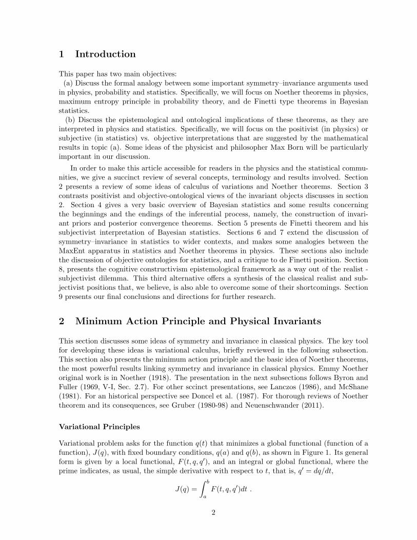
Variational problem asks for the function q(t) that minimizes a global functional (function of afunction), J(q), with fixed boundary conditions, q(a) and q(b), as shown in Figure 1. Its generalform is given by a local functional, F (t, q, q′), and an integral or global functional, where theprime indicates, as usual, the simple derivative with respect to t, that is, q′ = dq/dt,

J(q) =∫ b

aF (t, q, q′)dt .

2

1 1.5 22

2.5

3

1 1.5 2−0.3

0

0.3

1 1.5 22

2.5

3

Figure 1: Variational problem, q(x), η(x), q(x) + εη(x).

Euler-Lagrange Equation

Consider a ‘variation’ of q(t) given by another curve, η(t), satisfying the fixed boundary condi-tions, η(a) = η(b) = 0,

q = q(ε, t) = q(t) + εη(t) and

J(ε) =∫ b

aF(t, q(ε, t), q′(ε, t)

)dt .

A minimizing q(t) must be stationary, that is,

∂ J

∂ ε=

∂

∂ ε

∫ b

aF(t, q(ε, t), q′(ε, t)

)dt = 0 .

Since the boundary conditions are fixed, the differential operator affects only the integrand,hence

∂ J

∂ ε=∫ b

a

(∂ F

∂ q

∂ q

∂ ε+∂ F

∂ q′∂ q′

∂ ε

)dt

From the definition of q(ε, t) we have

∂ q

∂ ε= η(t) ,

∂ q′

∂ ε= η′(t) , hence ,

∂ J

∂ ε=∫ b

a

(∂ F

∂ qη(t) +

∂ F

∂ q′η′(t)

)dt .

Integrating the second term by parts, we get∫ b

a

∂ F

∂ q′η′(t)dt =

∂ F

∂ q′η(t)

∣∣∣∣ba

−∫ b

a

d

dt

(∂ F

∂ q′

)η(t)dt ,

where the first term vanishes, since the extreme points, η(a) = η(b) = 0, are fixed. Hence

∂ J

∂ ε=∫ b

a

(∂ F

∂ q− d

dt

∂ F

∂ q′

)η(t)dt .

Since η(t) is arbitrary and the integral must be zero, the parenthesis in the integrand must bezero. This is the Euler-Lagrange equation:

∂ F

∂ q− d

dt

∂ F

∂ q′= 0 .

3

If F does not depend explicitly on t, only implicitly through q and q′, Euler-Lagrange equationimplies

d

dt

(q′∂ F

∂ q′− F

)= q′′

∂ F

∂ q′+ q′

d

dt

∂ F

∂ q′− ∂ F

∂ t− ∂ F

∂ qq′ − ∂ F

∂ q′q′′ =

−q′(∂ F

∂ q− d

dt

∂ F

∂ q′

)− ∂ F

∂ t= 0 ⇒

(q′∂ F

∂ q′− F

)= const.

Hamilton’s Principle and Classical Mechanics

The Lagrangean of a classical mechanics system specified by generalized vector coordinates q(t),kinetic energy T (q, q′), and potential energy V (q, t), is defined as L(t, q, q′) = T (q, q′)− V (q, t).

Hamilton’s Principle states that, if a classical mechanics system is anchored at initial andfinal fixed positions q(a) and q(b), a < b, then the system follows the trajectory that minimizesit action. The action, J(q), is defined as the integral of the Lagrangean over time along thesystems’ trajectory,

J(q) =∫ b

aL(t, q, q′)dt .

Nother theorems establishes very general conditions under which the existence of a symmetryin the system, described by the invariance under the action of a continuous group, implies theexistence of a quantity that remains constant in the system’s evolution, that is, a conservationlaw, see for example Byron and Fuller (1969, V-I, Sec. 2.7).

As a first example, consider a Lagrangean L(t, q, q′) that does not depends explicitly of q.This situation reveals a symmetry: The system is invariant by a translation on the coordinateq. From Euler-Lagrange equation, it follows that the quantity p = ∂ F/∂ q′ is conserved. In thelanguage of classical mechanics, q would be called a cyclic coordinate, while p would be called ageneralized moment.

As a second example, consider a Lagrangean that does not depend explicitly on t. In thiscase, Euler-Lagrandge equation implies q′ ∂ L∂ q′ − L = E, where the constant E is interpretedas the system’s energy. Indeed, if the potential, V (q), is only function of the system position,and the kinetic energy is a quadratic form on the velocities, T =

∑i,j ci,jq

′iq′j , the last equation

assumes the familiar form E = 2T − L = T + V .

As a particular instance, consider a particle in a plane orbit around a radially symmetric andtime independent potential, L = m

2 (r′2 + r2θ′) − V (r). Since the Lagrangean does not dependexplicitly on θ, the system conserves its angular momentum, A, displayed in the next equation.Since the Lagrangean also does not depend explicitly on t, the system conserves its energy, E,

∂ L

∂ q′= mr2q′ = A , T + V =

m

2(r′2 + r2θ′) + V (r) = E .

These two constants of motion, A and E, are in fact a complete set of parameters for theparticle’s orbit, that is, these constants fully specify the possible orbits, as becomes clear bycombining the last equations into the following system of ordinary differential equations,

r′2 =

2m

(E − V (r))− m2r2

A, θ′ =

A

mr2.

4

3 Positivism vs. Objective Ontologies

In this section we discuss the ontological status of the constants or conserved quantities thatemerge from Noether’s theorem. For example, quantities E and A, energy or angular momen-tum, the parameters for the orbits of the central force system in the last subsection. What‘are’ these parameters? Are they something ‘real’? In following sections we discuss similar for-malisms in mathematical statistics, and raise similar questions concerning the ontological statusof parameters in statistical models.

3.1 Positivism, Subjectivism and Solipsism

According to the positivist school, closely related to the skeptical or solipsist traditions, the pri-mary physical quantities must be directly measurable, like time, position, etc. In the example athand, the variables of direct interest, corresponding to the primary physical quantities, describethe system’s trajectory, giving the time-evolution of the particle’s position, [r(t), θ(t)].

For the positivist school, quantities like A and E have a metaphysical character. The literalmeaning of the word meta-physical is just beyond-physical, designating entities that are notaccessible to our senses or, in our case, quantities that are not directly measurable. Therefore,from a positivist perspective, metaphysical entities have a very low ontological status, that is,they do not correspond to objects having a real existence in the world. Rather, they are ghostthat only exist inside our formalism.

In the example at hand, E and A constitute a very convenient index system for the collectionof all possible orbits, but that does not grant these quantities any real existence. On thecontrary, these quantities must be considered just as integration constants, useful variables inan intermediate step for the calculation of the system’s orbits. They can be used as convenientauxiliary variables, generating secondary or derived concepts, but that is all that they can everaspire to be. The physicist Max Born (1956, p.49,144,152) summarizes this position:

Positivism assumes that the only primary statements which are immediatelyevident are those describing direct sensual impressions. All other statements areindirect, theoretical constructions to describe in short terms the connections andrelations of the primary experiences. Only these have the character of reality. Thesecondary statements do not correspond to anything real, and have nothing to dowith an existing external world; they are conventions invented artificially to arrangeand simplify ‘economically’ the flood of sensual impressions.

[The] strictly positivistic standpoint: The only reality is the sense impressions.All the rest are ‘constructs’ of the mind. We are able to predict, with the help ofthe mathematical apparatus... what the experimentalist will observe under definiteexperimental conditions... But it is meaningless to ask what there is behind thephenomena, waves or particles or what else.

We have before us a standpoint of extreme subjectivism, which may rightly becalled ‘physical solipsism’. It is well-known that obstinately held solipsism cannotbe refuted by logical argument. This much, however, can be said, that solipsismsuch as this does not solve but evades the problem. Logical coherence is a purelynegative criterion; no system can be accepted without it, but no system is acceptablejust because it is logically tenable. The only positive argument in support of thisabstract type of ultra-subjectivism is... the belief in the existence of an externalworld is irrelevant and indeed detrimental to the progress of science.

5

3.2 Born Criticism of Positivism

The gnosiological sense of the word metaphysics has its roots in Aristotelic philosophy: In anutshell, it designates concepts that enable possible answers to why-questions, that is, meta-physical concepts are the basis for any possible answer ‘explaining why’ things are the waythey do. Hence, metaphysical concepts are at the core of metaphorical figures and explana-tion mechanisms, providing an articulation point between the empirical and the hypothetical, abridge from the rational and the intuitive, a link between calculation and insight. In this role,metaphysical concepts give us access to a ‘much deeper’ level of reality. Without metaphysicalconcepts, physical reasoning would be downgraded to merely cranking the formalism, either byalgebraic manipulation of the symbolic machinery or by sheer number crunching. Furthermore,metaphysical concepts are used to express metaphorical figures that constitute the basis of ourcommunication. These points are addressed by Max Born (1956, p.144,152):

Many physicists have adopted [the positivist] standpoint. I dislike it thoroughly...The actual situation is very different. All great discoveries in experimental physicshave been due to the intuition of men who made free use of models, which were forthem not products of the imagination, but representatives of real things. How couldan experimentalist work and communicate with his collaborators and his contem-poraries without using models composed of particles, electrons, nucleons, photons,neutrinos, fields and waves, the concepts of which are condemned as irrelevant andfutile?

However, there is of course some reason for this extreme standpoint. We havelearned that a certain caution is necessary in using these concepts... Modern theoriesdemand a reformulation. This new formulation is slowly evolving, but has probablynot reached a final expression.

The final lines of the last quotation address a distinct characteristic of modern science,namely, its dynamism, the rapid pace of its growth, the creation and reformulation of theories.However, formulating new theories implies creating new concepts and, sometimes, abandoningan old one. The frustration of finding out that some of the traditional good-old ‘things’ do not‘exist’, may be followed by the post-traumatic reaction of denying the existence of anything thatis not unequivocally perceived by direct sensorial experience. In this setting, the popularityof positivism or subjectivism may be understood as a first (although clumsy) reaction againstnaive realism. We believe that the two extreme epistemological positions of naive realism andsubjective solipsism can be seen as two tentatives of building an ontology based on a correspon-dence principle, as opposed to the approach taken in epistemological framework of cognitiveconstructivism. We will return to this theme at section 8.

3.3 Ontology by Invariance and Autonomy

The idea of founding an ontology on invariance properties has its origin in the Erlangen programof Felix Klein, see Klein (1893) and Hawkins (1984). His approach to geometry provided aunified treatment for Euclidean, non-Euclidean and Riemannian geometry, see Hawkins (1984)and Klein (2004). In Klein’s approach, the intrinsic properties of a geometric space is specifiedby a set of privileged actions, like a discrete or continuous group of possible transformations.Well known examples are the rigid translations and rotations of Euclidean geometry, the paralleltransport of Riemannian geometry, and so on. Moreover, the essential objects or properties insuch a geometry are characterized as invariants under the specified actions.

6

Furthermore, invariance suggests self-determination or autonomy: Invariance properties canbe interpreted as stating the irrelevance of peripheral peculiarities. For example, the irrelevanceof the particular coordinate system or reference frame being used (in a well defined class ofequivalence), the observer’s prior beliefs, etc. Hence, invariant objects are perceived to bedetached from any idiosyncratic condition, to stand by themselves, to be autonomous. MaxBorn (1956, p.158,163,104,51), summarizes this position as applied to build an ontology forphysical sciences:

I think the idea of invariant is the clue to a rational concept of reality, not onlyin physics but in every aspect of the world. The theory of transformation groupsand their invariants is a well established part of mathematics. Already in 1872 thegreat mathematician Felix Klein discussed in his famous ‘Erlanger Program’ theclassification of geometry according to this point of view; the theory of relativitycan be regarded as an extension of this program to the four-dimensional geometry ofspace-time. The question of reality in regard to gross matter has from this standpointa clear and simple answer.

Thus we apply analysis to construct what is permanent in the flux of phenomena,the invariants. Invariants are the concepts of which science speaks in the same wayas ordinary language speaks of ‘things’, and which it provides with names as if theywere ordinary things.

The words denoting things are applied to permanent features of observation orobservational invariants.

The invariants of [a] theory have the right to be considered as representationsof objects in the real world. The only difference between them and the objects ofeveryday life is that the latter are constructed by the unconscious mind, whereas theobjects of science are constructed by conscious thinking.

In the next sections we will analyze some formalisms for dealing with symmetry and in-variance in Bayesian statistics, their traditional subjectivist interpretations, and alternativeontological or objective interpretations based on the concepts of symmetry and invariance.

4 Bayesian Statistics

A standard model of (parametric) Bayesian statistics concerns an observed (vector) randomvariable, x, that has a sampling distribution with a specified functional form, p(x | θ), indexedby the (vector) parameter θ. This same functional form, regarded as a function of the freevariable θ with a fixed argument x, is the model’s likelihood function. In frequentist or classicalstatistics, one is allowed to use probability calculus in the sample space, but strictly forbiddento do so in the parameter space, that is, x is to be considered as a random variable, while θ isnot to be regarded as random in any way. In frequentist statistics, θ should be taken as a ‘fixedbut unknown quantity’ (whatever that means).

In the Bayesian context, the parameter θ is regarded as a latent (non-observed) randomvariable. Hence, the same formalism used to express credibility or (un)certainty, namely, prob-ability theory, is used in both the sample and the parameter space. Accordingly, the jointprobability distribution, p(x, θ) should summarize all the information available in a statisticalmodel. Following the rules of probability calculus, the model’s joint distribution of x and θcan be factorized either as the likelihood function of the parameter given the observation times

7

the prior distribution on θ, or as the posterior density of the parameter times the observation’smarginal density,

p(x, θ) = p(x | θ)p(θ) = p(θ |x)p(x) .

The prior probability distribution p0(θ) represents the initial information available about theparameter. In this setting, a predictive distribution for the observed random variable, x, is rep-resented by a mixture (or superposition) of stochastic processes, all of them with the functionalform of the sampling distribution, according to the prior mixing (or weights) distribution,

p(x) =∫θp(x | θ)p0(θ)dθ .

If we now observe a single event, x, it follows from the factorizations of the joint distributionabove that the posterior probability distribution of θ, representing the available informationabout the parameter after the observation, is given by

p1(θ) ∝ p(x | θ)p0(θ) .

In order to replace the ‘proportional to’ symbol, ∝, by an equality, it is necessary to dividethe right hand site by the normalization constant, c1 =

∫θ p(x | θ)p0(θ)dθ. This is the Bayes

rule, giving the (inverse) probability of the parameter given the data. That is the basic learn-ing mechanism of Bayesian statistics. Computing normalization constants is often difficult orcumbersome. Hence, especially in large models, it is customary to work with unormalized den-sities or potentials as long as possible in the intermediate calculations, computing only the finalnormalization constants. It is interesting to observe that the joint distribution function, takenwith fixed x and free argument θ, is a potential for the posterior distribution.

Bayesian learning is a recursive process, where the posterior distribution after a learningstep becomes the prior distribution for the next step. Assuming that the observations arei.i.d. (independent and identically distributed) the posterior distribution after n observations,x(1), . . . x(n), becomes,

pn(θ) ∝ p(x(n) | θ)pn−1(θ) ∝∏n

i=ip(x(i) | θ)p0(θ) .

If possible, it is very convenient to use a conjugate prior, that is, a mixing distribution whosefunctional form is invariant by the Bayes operation in the statistical model at hand. For example,the conjugate priors for the Normal and Multivariate models are, respectively, Wishart and theDirichlet distributions. The explicit form of these distributions is given in the next sections.

In the next two subsections we further discuss the ‘beginnings and the endings’ of theBayesian learning process, that is, we present some rationale for choosing the prior distribu-tion used to start the learning process, and some convergence theorems for the posterior as thenumber observations increases.

4.1 Fisher’s Metric and Jeffreys’ Prior

The Fisher Information Matrix, J(θ), is defined as minus the expected Hessian of the log-likelihood. The Fisher information matrix can also be written as the covariance matrix of forthe gradient of the same likelihood, i.e.,

J(θ) ≡ −EX∂ 2 log p(x | θ)

∂ θ2= EX

(∂ log p(x | θ)

∂ θ

∂ log p(x | θ)∂ θ

)8

The physicist Harold Jeffreys used the Fisher metric to define a class of prior distributions,proportional to the determinant of the information matrix,

p(θ) ∝ |J (θ)|1/2 .

Lemma: Jeffreys’ priors are geometric objects in the sense of being invariant by a continuousand differentiable change of coordinates in the parameter space, η = f(θ). The proof followsZellner (1971, p.41-54):

Proof:

J(θ) =[∂ η

∂ θ

]J(η)

[∂ η

∂ θ

]′, hence

|J (θ)|1/2 dθ =∣∣∣∣∂ η∂ θ

∣∣∣∣ |J (η)|1/2 = |J (η)|1/2 dη , Q.E.D.

Example: For the multinomial distribution,

p(y | θ) = n!∏m

i=1θxii

/∏m

i=1xi! , θm = 1−

∑m−1

i=1θi , xm = n−

∑m−1

i=1xi ,

L = log p(x | θ) =∑m

i=1xi log θi ,

∂ 2L

(∂ θi)2= −xi

θ2i

+xmθ2m

,∂ 2L

∂ θi∂ θj= −xm

θ2m

, i, j = 1 . . .m− 1 ,

−EX∂ 2L

(∂ θi)2=n

θi+

n

θm, −EX

∂ 2L

∂ θi∂ θj=

n

θm,

|J(θ)| = (θ1θ2 . . . θm)−1 , p(θ) ∝ (θ1θ2 . . . θm)−1/2 ,

p(θ |x) ∝ θx1−1/21 θ

x2−1/22 . . . θxm−1/2

m .

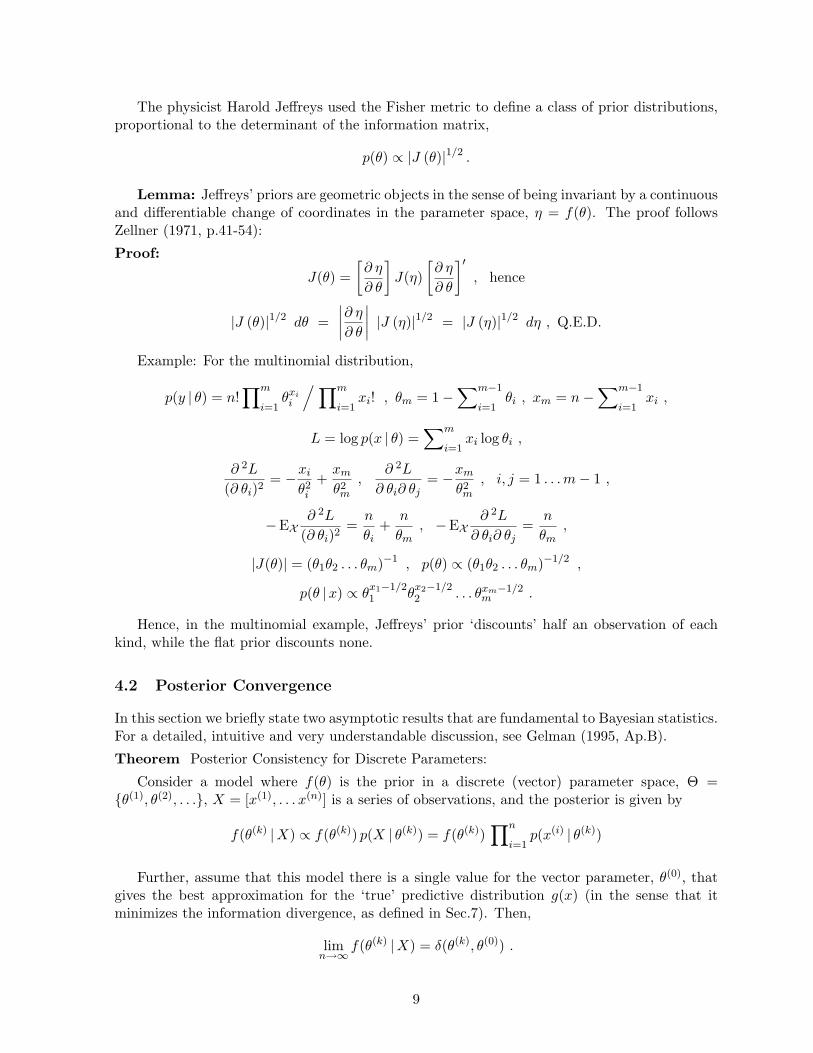
Hence, in the multinomial example, Jeffreys’ prior ‘discounts’ half an observation of eachkind, while the flat prior discounts none.

4.2 Posterior Convergence

In this section we briefly state two asymptotic results that are fundamental to Bayesian statistics.For a detailed, intuitive and very understandable discussion, see Gelman (1995, Ap.B).

Theorem Posterior Consistency for Discrete Parameters:

Consider a model where f(θ) is the prior in a discrete (vector) parameter space, Θ ={θ(1), θ(2), . . .}, X = [x(1), . . . x(n)] is a series of observations, and the posterior is given by

f(θ(k) |X) ∝ f(θ(k)) p(X | θ(k)) = f(θ(k))∏n

i=1p(x(i) | θ(k))

Further, assume that this model there is a single value for the vector parameter, θ(0), thatgives the best approximation for the ‘true’ predictive distribution g(x) (in the sense that itminimizes the information divergence, as defined in Sec.7). Then,

limn→∞

f(θ(k) |X) = δ(θ(k), θ(0)) .

9

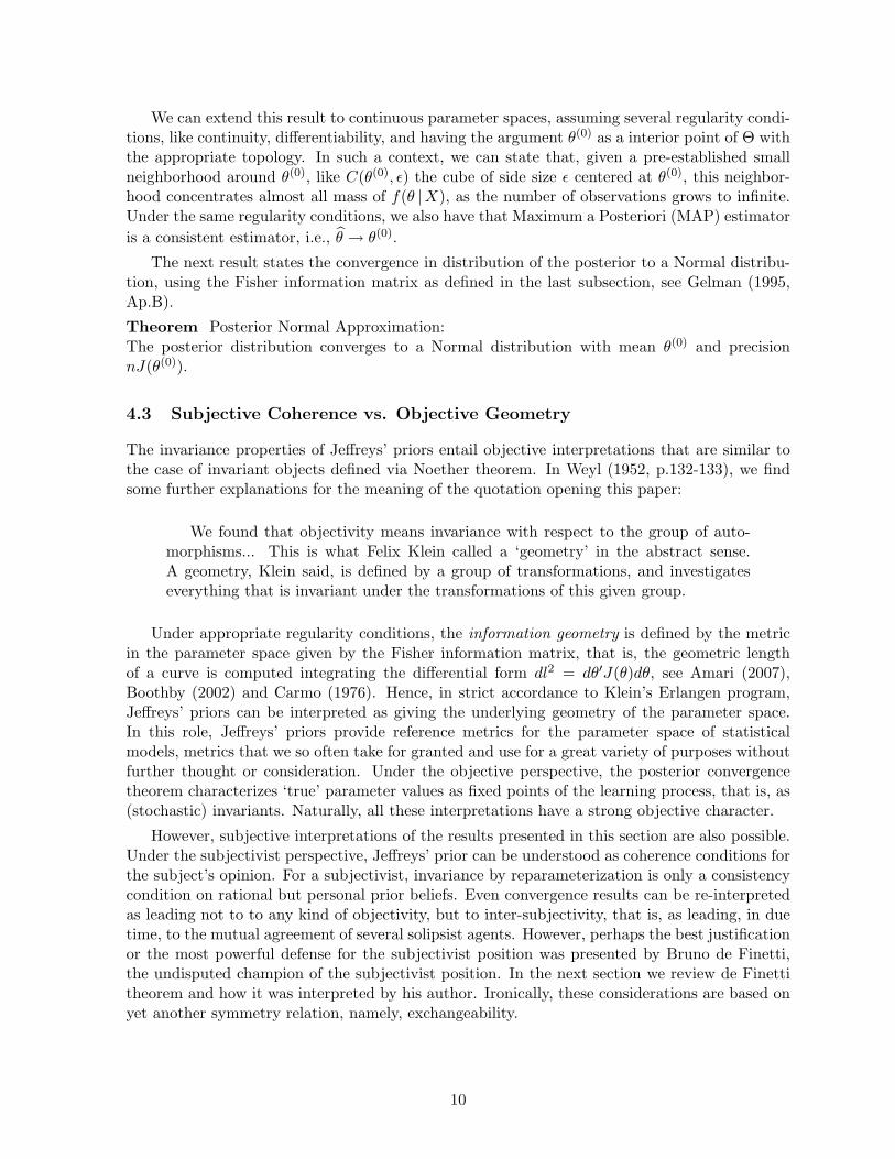
We can extend this result to continuous parameter spaces, assuming several regularity condi-tions, like continuity, differentiability, and having the argument θ(0) as a interior point of Θ withthe appropriate topology. In such a context, we can state that, given a pre-established smallneighborhood around θ(0), like C(θ(0), ε) the cube of side size ε centered at θ(0), this neighbor-hood concentrates almost all mass of f(θ |X), as the number of observations grows to infinite.Under the same regularity conditions, we also have that Maximum a Posteriori (MAP) estimatoris a consistent estimator, i.e., θ → θ(0).

The next result states the convergence in distribution of the posterior to a Normal distribu-tion, using the Fisher information matrix as defined in the last subsection, see Gelman (1995,Ap.B).

Theorem Posterior Normal Approximation:The posterior distribution converges to a Normal distribution with mean θ(0) and precisionnJ(θ(0)).

4.3 Subjective Coherence vs. Objective Geometry

The invariance properties of Jeffreys’ priors entail objective interpretations that are similar tothe case of invariant objects defined via Noether theorem. In Weyl (1952, p.132-133), we findsome further explanations for the meaning of the quotation opening this paper:

We found that objectivity means invariance with respect to the group of auto-morphisms... This is what Felix Klein called a ‘geometry’ in the abstract sense.A geometry, Klein said, is defined by a group of transformations, and investigateseverything that is invariant under the transformations of this given group.

Under appropriate regularity conditions, the information geometry is defined by the metricin the parameter space given by the Fisher information matrix, that is, the geometric lengthof a curve is computed integrating the differential form dl2 = dθ′J(θ)dθ, see Amari (2007),Boothby (2002) and Carmo (1976). Hence, in strict accordance to Klein’s Erlangen program,Jeffreys’ priors can be interpreted as giving the underlying geometry of the parameter space.In this role, Jeffreys’ priors provide reference metrics for the parameter space of statisticalmodels, metrics that we so often take for granted and use for a great variety of purposes withoutfurther thought or consideration. Under the objective perspective, the posterior convergencetheorem characterizes ‘true’ parameter values as fixed points of the learning process, that is, as(stochastic) invariants. Naturally, all these interpretations have a strong objective character.

However, subjective interpretations of the results presented in this section are also possible.Under the subjectivist perspective, Jeffreys’ prior can be understood as coherence conditions forthe subject’s opinion. For a subjectivist, invariance by reparameterization is only a consistencycondition on rational but personal prior beliefs. Even convergence results can be re-interpretedas leading not to to any kind of objectivity, but to inter-subjectivity, that is, as leading, in duetime, to the mutual agreement of several solipsist agents. However, perhaps the best justificationor the most powerful defense for the subjectivist position was presented by Bruno de Finetti,the undisputed champion of the subjectivist position. In the next section we review de Finettitheorem and how it was interpreted by his author. Ironically, these considerations are based onyet another symmetry relation, namely, exchangeability.

10

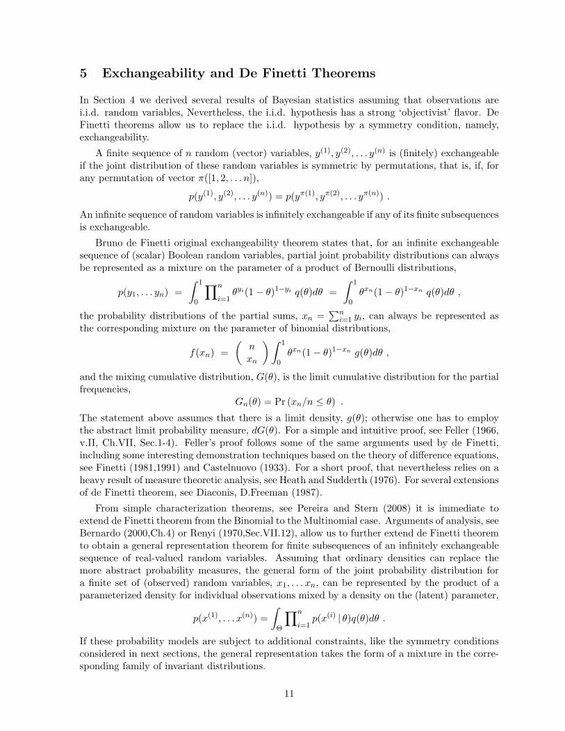
5 Exchangeability and De Finetti Theorems

In Section 4 we derived several results of Bayesian statistics assuming that observations arei.i.d. random variables, Nevertheless, the i.i.d. hypothesis has a strong ‘objectivist’ flavor. DeFinetti theorems allow us to replace the i.i.d. hypothesis by a symmetry condition, namely,exchangeability.

A finite sequence of n random (vector) variables, y(1), y(2), . . . y(n) is (finitely) exchangeableif the joint distribution of these random variables is symmetric by permutations, that is, if, forany permutation of vector π([1, 2, . . . n]),

p(y(1), y(2), . . . y(n)) = p(yπ(1), yπ(2), . . . yπ(n)) .

An infinite sequence of random variables is infinitely exchangeable if any of its finite subsequencesis exchangeable.

Bruno de Finetti original exchangeability theorem states that, for an infinite exchangeablesequence of (scalar) Boolean random variables, partial joint probability distributions can alwaysbe represented as a mixture on the parameter of a product of Bernoulli distributions,

p(y1, . . . yn) =∫ 1

0

∏n

i=1θyi(1− θ)1−yi q(θ)dθ =

∫ 1

0θxn(1− θ)1−xn q(θ)dθ ,

the probability distributions of the partial sums, xn =∑n

i=1 yi, can always be represented asthe corresponding mixture on the parameter of binomial distributions,

f(xn) =(

nxn

)∫ 1

0θxn(1− θ)1−xn g(θ)dθ ,

and the mixing cumulative distribution, G(θ), is the limit cumulative distribution for the partialfrequencies,

Gn(θ) = Pr (xn/n ≤ θ) .

The statement above assumes that there is a limit density, g(θ); otherwise one has to employthe abstract limit probability measure, dG(θ). For a simple and intuitive proof, see Feller (1966,v.II, Ch.VII, Sec.1-4). Feller’s proof follows some of the same arguments used by de Finetti,including some interesting demonstration techniques based on the theory of difference equations,see Finetti (1981,1991) and Castelnuovo (1933). For a short proof, that nevertheless relies on aheavy result of measure theoretic analysis, see Heath and Sudderth (1976). For several extensionsof de Finetti theorem, see Diaconis, D.Freeman (1987).

From simple characterization theorems, see Pereira and Stern (2008) it is immediate toextend de Finetti theorem from the Binomial to the Multinomial case. Arguments of analysis, seeBernardo (2000,Ch.4) or Renyi (1970,Sec.VII.12), allow us to further extend de Finetti theoremto obtain a general representation theorem for finite subsequences of an infinitely exchangeablesequence of real-valued random variables. Assuming that ordinary densities can replace themore abstract probability measures, the general form of the joint probability distribution fora finite set of (observed) random variables, x1, . . . xn, can be represented by the product of aparameterized density for individual observations mixed by a density on the (latent) parameter,

p(x(1), . . . x(n)) =∫

Θ

∏n

i=1p(x(i) | θ)q(θ)dθ .

If these probability models are subject to additional constraints, like the symmetry conditionsconsidered in next sections, the general representation takes the form of a mixture in the corre-sponding family of invariant distributions.

11

5.1 De Finetti Subjectivism

Bruno de Finetti is the founder of modern Bayesian statistics, and an outspoken advocate ofextreme subjectivism. In his lecture - Exchangeability, Induction and ‘Unknown’ Probabilities- Finetti (2008, Ch.8), he offers a synthesis of his interpretation of probability as subjectiveuncertainty in the context of the theorem presented in the last section:

Every time that probability is given by a mixture of hypotheses, with indepen-dence holding for each of them respectively, it is possible to characterize the inductiverelevance that results on the basis of [the mixture] equation in terms of exchangeabil-ity... [This] shows how the concept of exchangeability is necessary in order to expressin a meaningful way what is usually referred to as “independence with constant butunknown probability”. This expression is not correct because in fact (a) there is noindependence. (b) the probability is not constant because the composition of theurn being unknown, after learning the outcome of the draws, the probability of thevarious compositions is subject to variation.

Hence, according to de Finetti, the ‘objective’ i.i.d. condition is a mirage, a displacedreflection ‘outside’ of a more fundamental symmetry condition ‘inside’, namely, exchangeability.Naturally, for de Finetti, exchangeability is on the eyes of the beholder, expressing his or herown explicit or implicit opinions on how observational data should be correctly handled.

I.J.Good was another leading figure of the early days of the Bayesian revival movement.Contrary to de Finetti, Good has always been aware of the dangers of an extreme subjectivistposition. Some of his conclusions seem to echo Born’s arguments presented in section 1, see forexample Good (1983, Ch.8 Random Thoughts about Randomness, p.93):

Some of you might have expected me, as a confirmed Bayesian, to restrict the meaningof the word ‘probability’ to subjective (personal) probability. That I have not doneso is because I tend to believe that physical [objective] probability exists and is inany case a useful concept... The philosophical impact of de Finetti’s theorem is thatit supports the view that solipsism cannot be logically disproved. Perhaps it is themathematical theorem with most potential philosophical impact.

We intend to challenge de Finetti’s subjectivist view. However, before we can do so, we shallwiden the scope of our discussion, presenting probability distributions derived from symmetryconditions far more general than exchangeability.

6 Simple Symmetric Probability Distributions

Sections 6 and 7 present important results linking symmetry constraints and the functionalform of probability distributions. We follow the very simple approach to functional equationsof probability distributions in Aczel (1966). For related but more general and sophisticatedapproaches, see Diaconis (1988), Eaton (1989) and Viana (2008). These results will be importantin our philosophical discussions, but they will also help to answer a far more practical question:What family of distributions should we chose when specifying a statistical model?

12

6.1 Cauchy’s Functional Equations

In this subsection we introduce the additive and multiplicative forms of Cauchy functionalequation, since this functional equation will be used several times in the sequel.

Cauchy’s additive functional equation has the form

f(x+ y) = f(x) + f(y) .

The following argument from Cauchy (1821) shows that a continuous solution of this functionalequation must have the form

f(x) = cx .

Repeating the sum of the same argument, x, n times, we must have f(nx) = nf(x). Ifx = (m/n)t, then nx = mt and

nf(x) = f(nx) = f(mt) = mf(t) hence,

f(mnt)

=m

nf(t) ,

taking c = f(1), and x = m/n, it follows that f(x) = cx, over the rationals, x ∈ IQ. From thecontinuity condition for f(x), the last result must also be valid over the reals, x ∈ R. Q.E.D.

Cauchy’s multiplicative functional equation has the form

f(x+ y) = f(x)f(y) , ∀x, y > 0 , f(x) ≥ 0 .

The trivial solution of this equation is f(x) ≡ 0. Assuming f(x) > 0, we take the logarithm,reducing the multiplicative equation to the additive equation,

ln f(x+ y) = ln f(x) + ln f(y) , hence,

ln f(x) = cx , or f(x) = exp(cx) .

6.2 Radial Symmetry and the Gaussian Distribution

John Herschel (1850) gave the following derivation of the Gaussian or Normal distribution,concerning the distribution of errors in astronomical measurements. A few years later, JamesClerk Maxwell used the same arguments to derive the functional form of the probability distri-bution of molecular velocities in statistical physics. The derivation follows three simple steps,based on arguments of (1) independence, (2) radial symmetry and (3) normalization. For thesake of simplicity, we give the derivation using a two dimensional Cartesian coordinate system,x = [x1, x2].

Independence: Measurements on orthogonal axes should be independent,

f(x1)∐

f(x2)⇒ f(x) = f(x1)f(x2) .

Radial symmetry: Measurement errors should not depend on the current orientation of thecoordinate system. This step uses the exponential solution to Cauchy multiplicative functionalequation.

f(x) = f(x1)f(x2) = f(x21 + x2

2)⇒ f(x) ∝ exp(x21 + x2

2) = exp(||x||2) .

13

Normalization: The probability density must integrate to unity.∫f(x)dx1dx2 = 1⇒ f(x) =

a

πexp(−a||x||2) , a > 0 .

In the next section, we give a second derivation of this functional form based on the MaxEntformalism, given more general constraints on the first and second statistical moments, that is,the expectation vector and covariance matrix.

6.3 Homogeneous Discrete Markov Processes

We seek the general form of a homogeneous discrete Markov process. Let wk(t), for t ≥ 0, bethe probability of occurrence of exactly k events. Let us also assume the following hypotheses:

Time Locality: If t1 ≤ t2 ≤ t3 ≤ t4 then, the number of events in [t1, t2[ is independents ofthe number of events in [t3, t4[.

Time Homogeneity: The distribution for the number of events occurring in [t1, t2[ dependsonly on the interval length, t = t2 − t1.

From time locality and homogeneity, we can decompose the occurrence of no (zero) eventsin [0, t+ u[ as ,

w0(t+ u) = w0(t)w0(u) .

Hence, w0(t) must obey Cauchy’s functional equation, and

w0(t) = exp(ct) = exp(−λt) .

Since w0(t) is a probability distribution, w0(t) ≤ 1, and λ > 0.

Hence, v(t) = 1 − w0(t) = 1 − exp(−λt), the probability of one or more events occurringbefore t > 0, must be the familiar exponential distribution.

For k ≥ 1 occurrences before t+ u, the general decomposition relation is

wn(t+ u) =n∑k=0

wk(t)wn−k(u) .

Theorem (Renyi-Aczel): The Poisson distribution,

wk(t) = e−λt(λt)k/k! ,

is the (non trivial) solution of this system of functional equations under the rarity condition:The probability that an event occurs in a short time at least once is approximately equal to theprobability that it occurs exactly once, that is, the probability of simultaneous occurrences iszero. The general solution has the form of a mixture of Poisson processes, each one countingbursts of a fixed number of events. For the proof, by induction, see Aczel (1966, Sec.2.1-2.3).

Pereira and Stern (2008) present the characterization of the Multinomial by the Poissondistribution, and vice-versa. These characterizations allow us to interpret the exchangeabilitysymmetry characterizing a Multinomial processes in terms of the time homogeneity symmetryand superposition principle characterizing corresponding Poisson counting processes, and vice-versa. As observed by an anonymous referee, from a strict predictivist standpoint, our analogybetween de Finetti and Renyi-Aczel theorems is not fully complete, because an exogenous (to

14

the characterization) mixing distribution on the Poisson parameter has to be integrated intothe Bayesian inferencial model. In orther to present our analogy argument in full strength,the straight i.i.d. hypothesis for non-overlapping same-length intervals in Renyi-Aczel theoremshould be replaced by a weaker conditional i.i.d. hypothesis, given the asymptotic frequencyrate of the stochastic process. A direct characterization of the mixed Poisson process, based onsimilar symmetry conditions, can be found in Proposition 1.28 of Kallenberg (2005,p.66).

This example illustrates how there may be several alternative ways to formulate the funda-mental symmetries that characterize a given statistical model. The best choice may be dictatedby formal elegance and simplicity, or by the narrative or rhetorical context of the argumentsbeing supported by the statistical model at hand. Hence, in a scientific or philosophical debate,it is not at all surprising to see the participants flipping back and forth among alternative butequivalent symmetry conditions, according to their individual agendas and distinct perspectives.

7 Minimum Information or MaxEnt Principle

Section 1 presented Noether theorem as an apparatus that, based on the minimum action prin-ciple, takes a symmetry constraint and produces an invariant (physical) quantity. This sectionpresents the Maximum Entropy (MaxEnt) apparatus in a similar way, that is, given a symme-try condition, expressed by a suitable constraint equation, one can use the MaxEnt principleto derive the functional form of an invariant distribution. Using the MaxEnt apparatus, it ispossible to derive the functional form of many of the most probability distributions used instatistical models, see Kapur (1988). We also present Bregman algorithm as simple and elegantway to compute finite MaxEnt distributions even when no closed analytical form is available.The formulation of Bregman algorithm also provides a useful tool for validating the analyticform of generic MaxEnt solutions.

7.1 Maximum Entropy under Constraints

The origins of the entropy concept lay in the fields of Thermodynamics and statistical physics,but its applications have extended far and wide to many other phenomena, physical or not.The entropy of a probability distribution, H(p(x)), is a measure of uncertainty (or impurity,confusion) in a system whose states, x ∈ X , have p(x) as probability distribution. For detailedanalysis and further references, see Caticha (2008), Dugdale (1996), Khinchin (1953) and Stern(2008b,Ap.E). For the sake of simplicity, we present most of the following discussion in thecontext of a finite system, with states spanned by an indexed i ∈ {1, 2, . . . n}.

The Boltzmann-Gibbs-Shannon measure of entropy, defined as

Hn(p) = −In(p) = −∑n

i=1pi log(pi) = −Ei log(pi) , 0 log(0) ≡ 0

The opposite of the entropy, I(p) = −H(p), the Neguentropy, is a measure of Informationavailable about the system.

Shannon’s Inequality, a theorem that follows directly from the definition of entropy, can bestated as follows: If p and q are two distributions over a system with n possible states, andqi 6= 0, then the Information Divergence of p relative to q, In(p, q), is positive, except if p = q,when it is null,

In(p, q) ≡∑n

i=1pi log

(piqi

), In(p, q) ≥ 0 , In(p, q) = 0⇒ p = q

15

Shannon’s inequality motivates the use of the Information Divergence as a measure of (nonsymmetric) ‘distance’ between distributions. In statistical sciences, this measure is known asthe Kullback-Leibler distance. The denominations Directed Divergence or Cross Informationare used in Engineering.

Given a prior distribution, q, we would like to find a vector p that minimizes the InformationDivergence In(p, q), where p is under the constraint of being a probability distribution, andmaybe also under additional constraints over the expectation of functions taking values on thesystem’s states. In the specification of the constraints, A is an (m− 1)× n real matrix, and theproblem is formulated as

p∗ ∈ arg min In(p, q) , p ≥ 0 |1′p = 1 and Ap = b .

The solution p∗ is the Minimum Information Divergence distribution, relative to q, given theconstraints {A, b}. We can write the probability normalization constraint as a generic linearconstraint, including 1 and 1 as the m-th (or 0-th) rows of matrix A and vector b. So doing, wedo not need to keep any distinction between the normalization and the other constraints. In thischapter, the operators � e � indicate the point (element) wise product and division betweenmatrices of same dimension.

The Lagrangean function of this optimization problem, and its derivatives are:

L(p, w) = p′ log(p� q) + w′(b−Ap) ,

∂ L

∂ pi= log(pi/qi) + 1− w′A•,i ,

∂ L

∂ wk= bk −Ak,• p .

Equating the n+m derivatives to zero, we have a system with n+m unknowns and equations,giving viability and optimality conditions (VOCs) for the problem:

pi = qi exp(w′A•,i − 1

)or p = q � exp

((w′A)′ − 1

)Ak,• p = bk , p ≥ 0

We can further replace the unknown probabilities, pi, writing the VOCs only on w, the dualvariables (Lagrange multipliers),

hk(w) ≡ Ak,•(q � exp

((w′A)′ − 1

))− bk = 0

In the case of finite systems, the last form of the VOCs motivates the use of iterative algo-rithms of Gauss-Seidel type, solving the problem by cyclic iteration. In this type of algorithm,one cyclically ‘fits’ one equation of the system, for the current value of the other variables. Fora detailed analysis of this type of algorithm, see Censor and Zenios (1994, 1997), Elfving (1980),Fang et al. (1997), Garcia et al. (2002) and Iusem and Pierro (1987).

Bregman Algorithm:

Initialization: Take t = 0, w(t) ∈ Rm, and

p(t)i = qi exp

(w(t)′A•,i − 1

)Iteration step: for t = 1, 2, . . ., Take

k = (t mod m) and ν |ϕ(ν) = 0 , where

16

w(t+1) =[w

(t)1 , . . . w

(t)k−1, w

(t)k + ν, w

(t)k+1, . . . w

(t)m

]′p

(t+1)i = qi exp(w(t+1)′A•,i − 1) = p

(t)i exp(νAi,k)

ϕ(ν) = Ak,• p(t+1) − bk

From our discussion of Entropy optimization under linear constraints, it should be clearthat the minimum information divergence distribution for a system under constraints on theexpectation of functions taking values on the system’s states,

Ep(x)ak(x) =∫ak(x)p(x)dx = bk ,

(including the normalization constraint, a0 = 1, b0 = 1) has the form

p(x) = q(x) exp (−θ0 − θ1 a1(x)− θ2 a2(x) . . .)

Note that we took θ0 = −(w0−1), θk = −wk, and we have also indexed the state i by variable x,so to write the last equation in the standard form used in the statistical literature. Hence, thisform is a convenient way to check that several distributions commonly used in statistics can beinterpreted as minimum information (or MaxEnt) densities (relative to the uniform distribution,if not otherwise stated) given some constraints over the expected value of state functions. Forexample:

- The Binomial distribution is characterized as the distribution of maximum entropy fori ∈ {1 . . . n}, given the expected value of the mean, relative to the combinatorial prior C(n, i).

- The Normal distribution is characterized as the distribution of maximum entropy on Rn,given the expected values of its first and second moments, i.e., mean vector and covariancematrix.

- The Wishart distribution:

f(S | ν, V ) ≡ c(ν, V ) exp(ν − d− 1

2log(det(S))−

∑i,jVi,jSi,j

)is characterized as the distribution of maximum entropy in the support S > 0, given the expectedvalue of the elements and log-determinant of matrix S. That is, writing Γ′ for the digammafunction,

E(Si,j) = Vi,j , E(log(det(S))) =∑d

k=1Γ′(ν − k + 1

2

)- The Dirichlet distribution

f(x | θ) = c(θ) exp(∑m

k=1(θk − 1) log(xk)

)is characterized as the distribution of maximum entropy in the simplex support, x ≥ 0 |1′x = 1,given the expected values of the log-coordinates, E(log(xk)).

For the Multinomial distribution, the mean vector represents expected frequency rates, andthe combinatorial prior represents the equiprobability condition. The Multinomial distributionis only a function of accumulated counts, it is not dependent on the particular order of theoutcomes. Hence it represents exchangeable events.

For the Normal distribution, the mean represents a translation vector, and the coefficientsof the correlation matrix represent rotation angles. Translations and rotations constitute the

17

action group defining Euclidean geometry. In particular, Herchel’s isotropy and orthogonalitycondition is given by the zero mean vector and the identity correlation matrix, a symmetryconstraint that engenders the standard Normal distribution. Similar interpretations can begiven to the other distributions.

The Dirichlet and the Wishart distribution can be characterized as conjugate and invariantpriors for the first two distributions, or as MaxEnt distributions in their on right. Dirichlet-Multinomial and Normal-Wishart models, and many of its variations, like discrete Bayesiannetworks, regression, factor analysis, generalized linear models (GLIM), and combinations ofthe above, known as finite mixture models, encompass the most widely used classes of statisticalmodels. This is due to the formal convenience for mathematical manipulation offered by thesemodels, and also by the importance (in the target application) of the symmetries encoded bythese models. The next section should help to clarify this last statement.

8 Cognitive Constructivism

In the preceding sections, we have discussed several forms of symmetry found in statisticalmodels. However, it is a matter of constant debate whether these symmetries concern: (a) theobserver, (b) the observed phenomena an sich (in itself), or (c) the observation process. Thesethree possibilities are related to the epistemological frameworks of (a) subjectivism, skepticism,solipsism, etc. (b) naive or dogmatic forms of realism. (c) cognitive constructivism. Previ-ous sections discussed some aspects of the first two epistemological frameworks. This sectionsmakes additional considerations about these two frameworks and also introduces a third option,Cognitive Constructivism, or Cog-Con.

8.1 Objects as Eigen-Solutions

The Cog-Con framework rests upon Heinz von Forster’s metaphor of Objects as tokens foreigen-solutions. the key to Cog-Con ontology and metaphysics. The recursive nature of alearning system interacting with its environment produces recurrent states or stable solutions.Under appropriate conditions, such a (learned or known) solution, if presented to the system,will regenerate itself as a fixed point, an equilibrium or homeostatic state, etc. These arecalled eigen-values, eigen-vectors, eigen-functions, eigen-behaviors or, in general, eigen-solutions.The circular or cyclic characteristic of recursive processes and their eigen (auto, equilibrium,fixed, homeostatic, invariant, recurrent, recursive) -states are investigated in Foerster (2003)and Segal (2001). The concept of eigen-solution is the key to distinguish specific objects in thecognitive domain of a learning system. Objects are “tokens for eigen-solutions”. (A soccer ball issomething that interacts with a human in the exact way it is supposed to do for playing soccer.)Eigen-solutions can also be tagged or labeled by words, and these words can be articulatedin language. Of course, the articulation rules defined for a given language, its grammar andsemantics, only make the language useful if they somehow correspond to the composition rulesfor the objects the words stand for.

Moreover, von Foerster establishes four essential attributes of eigen-solutions: Eigen-valuesare ontologically discrete, stable, separable and composable. It is important to realize that,in the sequel, the term ‘discrete’, used by von Foerster to qualify eigen-solutions in general,should be replaced, depending on the specific context, by terms such as lower-dimensional,precise, sharp, singular etc. In several well known examples in exact sciences, these four essentialproperties lead to the concept of basis, basis of a finite vector space, like in linear algebra, basis

18

of a Hilbert space, like in Fourier or Wavelet analysis, or more abstract settings, like basis formatroid structure, generators for an algebraic group, etc. Nevertheless, the concept of eigen-solution and its four essential properties is so important in the Cog-Con framework, that it isused as a fundamental metaphor in far more general, and not necessarily formalized, contexts.For detailed interpretations of the of these four essential attributes on eigen-solutions in thecontext of Bayesian learning systems, see Stern (2007a,b, 2008a,b). For a formal derivation ofcompositionality properties in the FBST context, see Borges and Stern (2007).

8.2 Semantics by Construction and by Correspondence

In this subsection we further investigate some consequences of the Cog-Con perspective onobjects and their representation in language, contrasting it with more traditional approaches,based on dyadic cuts and subsequent correspondences. Correspondence approaches start bymaking a distinction that cuts the world in two, and then choose or decide if objects are correctlyplaced ‘in here’ or ‘out there’: Are they internal concepts in a given system or are they externalentities in the environment? Do they belong to the ‘subjective’ or ‘upper’ world of the mind,spirit, intuitive thought etc. or do they belong to ‘reality’ or ‘lower’ world of the body, matter,etc.?

The predetermined cut splitting the world in two also suggests two natural alternative waysto climb the epistemological mountain: Either the correct ideas above are those correspondingto the ‘reality’ below, or the correct things below are those corresponding to the ‘good’ ideasabove, etc. The existence of true and static correspondence principle is a necessary pre-requisite,but there are different ways to establish the connection, or to learn it (or to remember it). Anempiricist diligently observes the world, expecting his reward to be paid in current scientificknowledge that can, in turn, be used to pay for convenient tools to be used in technologicalenterprises. A dogmatic idealist works hard at his metaphysical doctrine, in order to secure agood spot at the top, expecting to have an easy ride sliding down the epistemological road.

The dyadic correspondence approach is simple and robust. It can be readily adapted tomany different situations and purposes. It also has attractive didactic qualities, being easyto understand and to teach. The dyadic correspondence approach has low entrance fees andlow maintenance costs, as long as one understands that the assumption of a predeterminedcorrespondence makes the whole system essentially static. Its major weakness relates to thisrigidity. It is not easy to consider new hypothesis or original concepts, and even harder to handlethe refutation or the dismissal of previously accepted ones. New world orders always need tobe, at least conceptually, proven afresh or build up from scratch.

In Cognitive Constructivism, language can be seen as a third pole in the epistemologicalframework, a third element that can play the role of a buffer, moderating or mitigating theinteraction of system and environment, the relation of theory and experiment, etc. After all,it is only in language that it is possible to enunciate statements, that can then be judged fortruthfulness or falsehood. Moreover language gives us a shelf to place our objects (represen-tations of eigen-solutions), a cabinet to store these (symbolic) tokens. Even if the notion ofobject correspondence, to either purely internal concepts to a given system or to strictly exter-nal entities in the environment, is inconsistent with the Cog-Con framework, this framework isperfectly compatible with having objects re-presented as symbols in one or several languages.This view is very convenient and can be very useful, as long as we are not carried away, andstart attributing to language magic powers capable of creating ex-nihilo the world we live in.As naive as this may seem, this is a fatal mistake made by some philosophers in the radical

19

constructivist movement, see Stern (2005).

The Cog-Con approach requires, from the start, a more sophisticated construction, butit should compensate this trouble with the advantage of being more resilient. Among ourgoals is escaping the dilemmas inherent to predetermined correspondence approaches, allowingmore flexibility, providing dynamic strength and stability. In this way, finding better objects,representing sharper, stabler, easier to compose, or more generally valid eigen-solutions (or evenbetter representations for these objects in the context of a given system), does not automaticallyimply the obliteration of the old ones. Old concepts or notations can be replaced by betterones, without the need ever being categorically discredited. Hence, theories have more roomto continuously grow and adapt, while a concept at one time abandoned may be recycled if its(re)use is convenient at a later opportunity. In this way, the Cog-Con epistemological frameworknaturally accommodates dynamic concepts, change of hypotheses and evolution of theories, allso characteristic of modern science.

9 Conclusions and Further Research

When Bayesian statistical models are examined in the Cog-Con framework, the role played by themodel’s parameters becomes clear: They are (converging to) eigen-solutions of that statisticalmodel in the process of information acquisition by the incorporation of observational data. Theseeigen-solution are (in the limit, stochastic) invariants of the Bayesian learning process. As such,they have a compelling objective character, according to Herman Weyl’s quotation opening thisarticle. The precision aspect of the quality of these eigen-solution, that is, its objectivity, can beaccessed by the current posterior density. Hence, we can also access the objective truthfulnessof more general hypotheses, stated as equations on the parameters. The FBST - Full BayesianSignificance Test, was designed having this specific purpose in mind, see Borges and Stern (2007)and Pereira et al. (2008).

Frequentist statistics categorically forbids probabilistic statements in the parameter space.De Finettian subjectivist interpretation of Bayesian statistics ‘justifies’ the use of prior andposterior distributions for the parameters, but their role is to be used as nothing more thenintegration variables in the process of computing predictive distributions. In a very positivistspirit, like any other non directly observable or latent quantity, parameters are labeled as meta-physical entities, and given a very low ontological status. Finally, in the Cog-Con interpretationof Bayesian statistics, parameters can take their rightful place on the center stage of the infer-ential process. They are not just auxiliary variables, but legitimate objects of knowledge, thatcan be properly used in true bearing statements. We claim that the last situation correspondsto what a scientist naturally finds, needs and wants in the practice of empirical science.

Ontological frameworks based on correspondence semantics seem to be particularly inappro-priate in quantum mechanics. We believe that many of the arguments and ideas presented inthis paper can be re-presented, even more emphatically, for statistical models concerning exper-imental measurements in this realm. The formal analogies between the symmetry argumentsand their use in statistics and physics is even stronger in quantum mechanics than in the caseof classical physics, see Gross (1995), Houtappel et al. (1965), Fleming (1979) and Wigner(1967,1968). For example, the idea of eigen-solution, that already plays a very important rolein the epistemology of classical physics, see for example Stern (2008b), plays an absolutelypreponderant role in quantum mechanics. Furthermore, the quantum mechanics superpositionprinciple makes the use of mixtures of basic symmetric solutions as natural (and necessary) in

20

quantum mechanics as they are in statistics. Moreover, quantum mechanics theory naturallyleads to interpretations that go beyond the classical understanding of probability as ‘uncertaintyabout a well defined but unknown state of nature’. As stated by Born (1956,p.168), in quantummechanics “the true physical variable is the probability density”.

Perhaps Born’s statement ending the last paragraph is also pertinent in application ar-eas (sometimes derogatorily) labeled ‘soft’ science. In the context of physics and other ‘hard’sciences, we search for anchors that can hold to the very fabric of existence, which can griprock-bottom reality, or provide irreducible elements that can be considered as basic constituentsor components of a multitude of derived complex systems. In this context, this article arguedthat the objective perspective offered by the Cog-Con epistemological framework is far superiorto the strict subjective (or at most inter-subjective) views of the decision theoretic epistemolog-ical framework of traditional Bayesian statistics. Meanwhile, in the context of ‘soft’ sciences,like marketing, psychology or sociology, the subjective and inter-subjective views of traditionalBayesian statistics may not contradict but rather complement the objective perspective offeredby Cog-Con. We intend to explore this possibility as a second path of future research.

References

- J.Aczel (1966). Lectures on Functional Equations and their Applications. NY: Academic Press.- S.I.Amari (2007). Methods of Information Geometry. American Mathematical Society.- W.Boothby (2002). An Introduction to Differential Manifolds and Riemannian Geometry. NY: Aca-demic Press.- W.Borges, J.M.Stern (2007). The Rules of Logic Composition for the Bayesian Epistemic e-values.Logic Journal of the IGPL, 15, 5-6, 401-420. doi:10.1093/jigpal/jzm032 .- M.Born (1949). Natural Philosophy of Cause and Chance. Oxford: Clarendon Press.- M.Born (1956). Physics in my Generation. London: Pergamon Press.- F.W.Byron Jr., R.W.Fuller (1969). Mathematics of Classical and Quantum Physics. Reading, MA:Addison-Wesley.- Y.Censor, S.A.Zenios (1997). Parallel Optimization: Theory, Algorithms, and Applications. NY: OxfordUniv.Press.- G.Castelnuovo (1933). Calcolo delle Probabilita. Bologna: N.Zanichelli.- A. Caticha (2008). Lectures on Probability, Entropy and Statistical Physics. Tutorial book for MaxEnt2008, The 28th International Workshop on Bayesian Inference and Maximum Entropy Methods in Scienceand Engineering. July 6-11 of 2008, Boraceia, Sao Paulo, Brazil.- P.Diaconis, D.Freeman (1987). A Dozen de Finetti Style Results in Search of a Theory. Ann. Inst.Poincare Probab. Stat., 23, 397–423.- P.Diaconis (1988). Group Representation in Probability and Statistics. Hayward: IMA.- M.G.Doncel, A.Hermann, L.Michel, A.Pais (1987). Symmetries in Physics (1600-1980). Seminarid’Historia des les Ciences. Universitat Autonoma de Barcelona.- J.S.Dugdale (1996). Entropy and Its Physical Meaning. London: Taylor and Francis.- M.L.Eaton (1989). Group Invariance Applications in Statistics. Hayward: IMA.- T.Elfving (1980). On Some Methods for Entropy maximization and Matrix Scaling. Linear algebra andits applications, 34, 321-339.- S.C.Fang, J.R.Rajasekera, H.S.J.Tsao (1997). Entropy Optimization and Mathematical Programming.Dordrecht: Kluwer.- B.de Finetti (1981) Scritti 1926-1930. Padova: CEDAM. p.268-315, Funzione Caratteristica de unFenomeno Aleatorio. Also in Memorie della R.Accdemia dei Lincei, 1930, v.IV,p.86-133.- B.de Finetti (1991). Scritti 1931-1936. Bologna: Pitagora. p.323-326, Independenza Stocastica edEquivalenza Stocastica. Also in Atti della Societa Italiana per il Progresso delle Scienze, XXII Riunione,Bari, 1933, v.II,p.199-202.- B.de Finetti, A.Mura ed. (2008). Philosophical Lectures on Probability. Synthese Library v.340.

21

Heidelberg: Springer.- W.Feller (1966). An Introduction to Probability Theory and Its Applications (2nd ed.), V.II. NY: Wiley.- H.Fleming (1979). As Simetrias como Instrumento de Obtencao de Conhecimento. Ciencia e Filosofia,1, 99–110.- M.V.P.Garcia, C.Humes, J.M.Stern (2002). Generalized Line Criterion for Gauss Seidel Method. Jour-nal of Computational and Applied Mathematics, 22, 1, 91-97.- A.Gelman, J.B.Carlin, H.S.Stern, D.B.Rubin (2003). Bayesian Data Analysis, 2nd ed. NY: CRC.- D.J.Gross (1995). Symmetry in physics: Wigner’s legacy Physics Today, 48, 12, 46-50.- B.Gruber et al. edit. (1980–98). Symmetries in Science, I–X. NY: Plenum.- Th.Hawkins (1984). The Erlanger Programm of Felix Klein: Reflections on Its Place In the History ofMathematics. Historia Mathematica, 11, 442-70.- D.Heath, W.Sudderth. De Finetti Theorem on Echangeable Variables. The American Statistician,30,4,188-189.- R.Houtappel, H.van Dam, E.P.Wigner (1965). The Conceptual Basis and Use of the Geometric Invari-ance Principles. Reviews of Modern Physics, 37, 595–632.- E.T.Jaynes (2003). Probability Theory: The Logic of Science. Cambridge Univ.Press- O.Kallenberg (2005). Probabilistic Symmetries and Invariance Principles. NY: Springer.- J.N.Kapur (1989). Maximum Entropy Models in Science and Engineering. New Delhi: John Wiley.- A.I.Khinchin (1953). Mathematical Foundations of Information Theory. NY: Dover.- F.Klein (1893). Vergleichende Betrachtungen uber neuere geometrische Forschungen. MathematischeAnnalen, 43, 63-100. Transl.as A comparative review of recent researches in geometry, Bull.N.Y.Math.Soc.(1893) 2, 215–249.- F.Klein (2004) Elementary Mathematics from an Advanced Standpoint: Geometry. N.Y. Dover.- C.L.Lanczos (1986). The Variational Principles of Mechanics. Noether’s Invariant Variational Prob-lems, Appendix II, p.401-405. NY: Dover.- E.J.McShane (1981). The Calculus of Variations. Ch.7, p.125-130 in: J.W.Brewer, M.K.Smith (1981).Emmy Noether. Marcel Dekker.- D.E.Neuenschwander (2011). Enny Noether’s Wonderful Theorem. Baltimore: Johns Hopkins Univ.Press.- E.Noether (1918). Invariante Varlationsprobleme. Nachrichten der Konighche Gesellschaft der Wis-senschaften zu Gottingen. 235–257. Transl. Transport Theory and Statistical Physics, 1971,1,183–207.- M.P.do Carmo (1976). Differential Geometry of Curves and Surfaces. NY: Prentice Hall.- C.A.B.Pereira, J.M.Stern (2008). Special Characterizations of Standard Discrete Models. REVSTATStatistical Journal, 6, 3, 199-230.- C.A.B.Pereira, S.Wechsler, J.M.Stern (2008). Can a Significance Test be Genuinely Bayesian? BayesianAnalysis, 3, 1, 79-100.- A.Renyi (1970). Probability Theory. Amsterdam: North-Holland.- J.M.Stern (2007a). Cognitive Constructivism, Eigen-Solutions, and Sharp Statistical Hypotheses. Cy-bernetics and Human Knowing, 14, 1, 9-36.- J.M.Stern (2007b). Language and the Self-Reference Paradox. Cybernetics and Human Knowing, 14,4, 71-92.- J.M.Stern (2008a). Decoupling, Sparsity, Randomization, and Objective Bayesian Inference. Cybernet-ics and Human Knowing, 15, 2, 49-68.- J.M.Stern (2008b). Cognitive Constructivism and the Epistemic Significance of Sharp Statistical Hy-potheses. Tutorial book for MaxEnt 2008, The 28th International Workshop on Bayesian Inference andMaximum Entropy Methods in Science and Engineering. July 6-11 of 2008, Boraceia, Sao Paulo, Brazil.- M.Viana (2008). Symmetry Studies: An Introduction to the Analysis of Structured Data in Applications.Cambridge Univ.Press.- S.Wechsler (1993). Exchangeability and Predictivism. Erkenntnis, 38,3,343-350.- H.Weyl (1989). Symmetry. Princeton Univ.Press.- E.P.Wigner (1968). Symmetry Principles in Old and New Physics. Bull.Amer.Math.Soc. 74, 5, 793-815.- E.P.Wigner (1967). Symmetries and Reflections. Bloomington: Indiana University Press. Includingthe reprint of Wigner (1964). Symmetry and Conservation Laws. Proc.Natl.Acad.Sci.USA. 51,5,956-965.

22