BNL .- 64489 CAP - 167-97C

SYMPLECTIC INTEGRATION*

Zohreh Parsa Brookhaven National Laboratory

Upton, NY 11973

and

Etienne Forest National Laboratory for High Energy Physics

Tsukuba, Japan

* T h i s w o r k w a s p e r f o r m e d under the a u s p i c e s of the U.S. D e p a r t m e n t of E n e r g y u n d e r C o n t r a c t N o . DE-AC02-76CHO0016.

May 1997

Submitted to 1% Ad;nnced ICFA B m Dynnmics Workshop on Nonlinear and &Uective P h e M m e ~ in Beam Physics: %oty and ErperimenLF', Arcidossa, Iw, &pi. 24.19%.

Symplectic Integration

Zohreh ParsalJ and- Etienne Forest"'

Brookhauen National Laboratory, Upton, New York Institute for Theoretical Physics, Santa Barbara, Ccilifornia

3Nat2'onal Laboratory for High Energy Physics, Tsukuba, Japan .

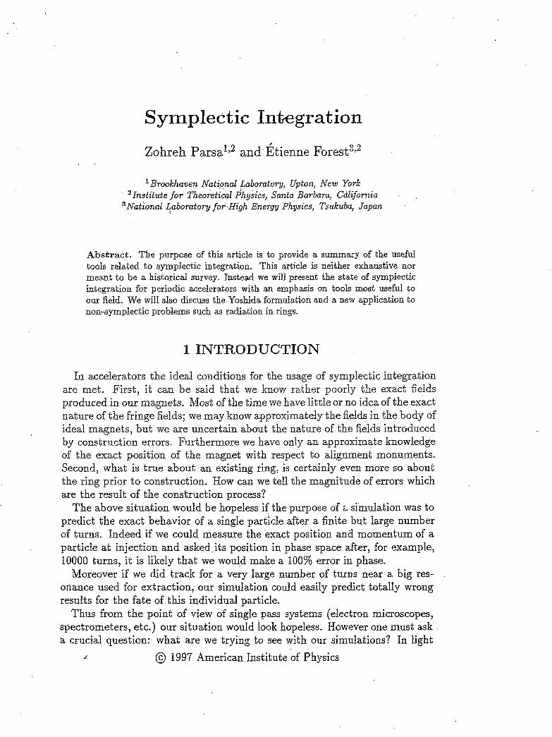
Abstract. The purpose of this article is to provide a summary of the useful tools related to symplectic integration. This article is neither exhaustive nor meant to be a historical survey. Instead we will present the state of symplectic integration for periodic accelerators with an emphasis on tools most useful to our field. We will also discuss the Yoshida formulation and a new application to non-symplectic problems such as radiation in rings.

I. INTRODUCTION

In accelerators the ideal conditions for the usage of symplectic integration are met. First, it can be said that we know rather poorly the exact fields produced in OUT magnets. Most of the time we have little or no idea of the exact nature of the fringe fields; we may know approximately the fields in the body of ideal magnets, but we are uncertain about the nature of the fields introduced by construction errors. Furthermore we have only an approximate knowledge of the exact position of the magnet with respect to alignment monuments. Second, what is true about an existing ring, is certainly even more so about the ring prior to construction. How can we tell the magnitude of errors which are the result of the construction process?

The above situation would be hopeless if the purpose of i simulation was to predict the exact behavior of a single particle after a finite but large number of turns. Indeed if we could measure the exact position and momentum of a particle at injection and asked its position in phase space after, for example, 10000 turns, it is likely that we would make a 100% error in phase.

Moreover if we did track for a very Iarge number of turns near a big res- onance used for extraction, our simulation could easily predict totally wrong results for the fate of this individual particle.

Thus from the point of view of single pass systems (electron microscopes, spectrometers, etc.) our situation would look hopeless. However one must ask a crucial question: what are we trying to see with our simulations? In light

,r @ 1997 American Institute of Physics

of such a question it becomes clear that symplectic integration is an ideal and indispensible tool for rings while it may not be a useful tool for single pass systems where the fate and exact position of a ray is of paramont importance.

,

Symplectic integration works best when ye are most interested in the ba- sic topology of phase space and on the effect of changes of the operating parameters on this basic topology. The symplectic condition has a tremen- dous influence on the shape of phase space. Many structures which are found in nonsymplectic systems are forbidden by the symplectic condition: sinks, strange attractors, limit cycles, etc. Symplectic integration allows us to per- form simulations in which these structures cannot appear. The preservation of the topological structure of phase space by a nonsymplectic integrator re- quires a large number of integration steps and/or a high order integrator. For an ordinary integrator, the preservation of the syrnplectic condition is tied to its accuracy. Thus with a symplectic scheme we can take advantage of the fact that the basic topology does not seem to depend much on the model, provided certain structural properties are held constant (tunes, chromaticity, etc.). In a sense when using a symplectic integrator it is useful, if not essential, to re- interpret the integrator as a different model of the ring. If one fails to do this, then one is tempted to increase the number of integration steps until the inte- grator produces the tunes (chromaticities, etc.) of the exact solution. Instead one should re-fit the parameters of the ring so that the integrator behaves in a way similar to the exact solution with a number of integration steps as small as possible. This is the basic philosophy of symplectic integration applied to ring dynamics’.

In closing this introduction we point out that symplectic integration is also important in electron ring simulations with classical radiation. Indeed the effect of radiation though being small OD a magnet by magnet basis, is im- portant and should be included on top of a symplectic scheme. Otherwise its effect would be swamped by integration errors.

‘

2 ExmrcrT SYMPLECTIC INTEGRATION

We mentioned that this primer is geared towards accelerator dynamics. Therefore we wi l cover mostly explicit symplectic integration. It is worth noting that all the so-called “kick codes” which use matrices to represent “lin- ear elements” (quadrupoles and bends) and thin lens kicks for the multipoIes are second order explicit symplectic integrators. These integrators require the

‘1 This is also partially R. Talman’s point of view: “Instead of using approximate formulae to perform tracking through “exact” (Le. thick) elements, it is possible to perform exact tracking through (i.e. thin) elements. The approximation can be improved by breaking thick elements into several thin elements. Long-term precision in such a program is only compromised by round-off error in the computer.” See reference [l].

c

ability to split the Hamiltonian into exactly solvable parts, for example ma- trices and kicks in standard kick codes. It may be noted that the construction of explicit symplectic integrators of higher order was addressed in the early eighties by R. Ruth C2]. However, in this papef, we will follow the more recent approach of H. Yoshida because of its simplicity and greater generality.

.

2.1 Exact Tracking through Inexact Elements

Consider the following s-dependent Hamiltonian which may represent a drift followed by a combined function quadrupole-sextupole magnet:

(1)

where the functions k2(s) and k3(s) have period 1. Thus it suffices to define them between 0 and, 1:

1 k ; = O f o r O < s < -

2

and

We can plot the exact solution for this system at s = 3/4. This is depicted on figure 1.

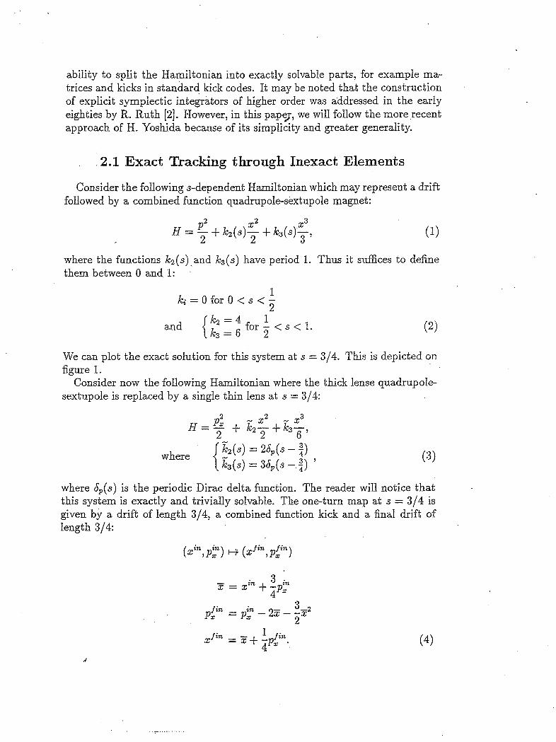
Consider now the following Hamiltonian where the thick lense quadrupole- sextupole is replaced by a single thin lens at s = 3/4:

where Sp(s) is the periodic Dirac delta function. The reader will notice that this system is exactly and trivially solvable. The one-turn map at s = 3/4 is given by a drift of length 3/4, a combined function kick and a final drift of length 3/4:

( p p F ) ( x f i n ? X p n )

f

. . , , __ , . . ... . -. - .. .

0.00

-1 -00 0.00

FIGURE 1. Exact Tracking

1 .oo

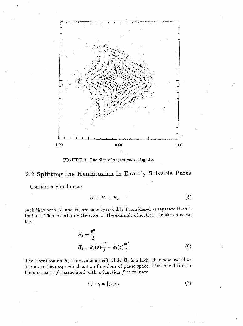
One can look at this new map in two different ways; the second way will be addressed in the next section. First, the thick “combined function quadrupole- sextupole” has been replaced by a thin quadrupole-sextupole at s = 3/4. This new system has a phase plot given by figure 2, on which it can be seen that the topology is drastically different from that of the original system depicted on figure 1. In fact while the tune u of the exact solution is 0.2309, the impulsive system is exactly on u = 1/4. How do we improve this? One could increase the number of integration steps until the system produces nearly the right phase space topology, but this would be an in inefficient usage of symplectic integration. Instead one should consider the integrator to be the exact lattice and readjust the parameters of the system. For example, if we fit the tune to 0.2309 by adjusting the quadrupole strength kz to 3.522 one obtains the topology of figure 3. It is clear that we are doing much better now. To further improve our results, it would be customary in an accelerator to increase the number of thin lenses by one and to refit again. It is important to redefine the element as being the integrator itself. In the next section we will reinterpret the example of this section in light of explicit symplectic integration.

...................... ........ . . . . . . . _, - .- . _. . - - ._ _-_ . .- .- . - _. -

..... . . .

0.00

One can look at this new map in two different ways; the second way will be addressed in the next section. First, the thick “combined function quadrupole- sextupole” has been replaced by a thin quadrupole-sextupole at s = 3/4. This new system has a phase plot given by figure 2, on which it can be seen that the topology is drastically different from that of the original system depicted on figure 1. In fact while the tune u of the exact solution is 0.2309, the impulsive system is exactly on v = 1/4. How do we improve this? One could increase the number of integration steps until the system produces nearly the right phase space topology, but this would be an in inefficient usage of symplectic integration. Instead one should consider the integrator to be the exact lattice and readjust the parameters of the system. For example, if we fit the tune to 0.2309 by adjusting the quadrupole strength kz to 3.522 one obtains the topology of figure 3. It is clear that we are doing much better now. To further improve our results, it would be customary in an accelerator to increase the number of thin lenses by one and to refit again. It is important to redefine the element as being the integrator itself. In the next section we will reinterpret the example of this section in light of explicit symplectic integration.

. .

I l l l l l l l l l l l l l l l l l l l

-1 .oo 0.00 I .oo

FIGURE 2. One Step of a Quadratic Integrator

2.2 Splitting the Hamiltonian in Exactly Solvable Parks

Consider a Hamiltonian

such that both HI and H2 are exactly solvable if considered as separate Hamil- tonians. This is certainly the case for the example of section . In that case we have

The Hamiltonian HI represents a drift while Hz is a kick. It is now useful to introduce Lie maps which act on functions of phase space. First one defines a Lie operator : f : associated with a function f as follows:

J

. . . . . . . .

. . . --- . . -.. , .; .. : ' 8 '

. .. . ..~ .%

f .....

-1.00 1 1 1 1 1 1 1 1 1 1 1 1 1 1 I l l I ,

-1.00 0.00 1 .oo

FIGURE 3. One Step of a Quadratic Integrator Refitted

where g is an arbitrary function of phase space. Using this definition of a Lie map for the drift HI, the map MI is constructed:

This map, unlike the usual transfer map, acts on functions of phase space. It describes the evolution of a function. The usual transfer map is regained by letting MI act on the functions x and p i.e. the projection functions of phase space (the identity transfer map):

P2 ~ l ( x , p ) = exp(: -s- : ) (x,p) 2

= (eip(: -s- P2 : )12:,exp(: -s- P2 : )p) 2 2

The above Lie representation is then used to reinterpret our integrator scheme. One can show that the exact Lie map for the combined function "quadrupole- sextupole" is given by the formula

M = exp (-t : Hl + H2 :) . (10)

This operator can be approximated as follows:

S ~ ( s ) 21 exp (-? : H~ :j exp (- s / H ~ :j exp (-; : H~ :>

= S2(s). (11)

Of. course this formula would be exact if the operators : HI : and : 112 : did commute. But then, by assumption, we would have an exact solution by solving for the map due HI and theo for the map due to H2, There would be no need for an integration scheme. Thus it is fair to assume that : HI : and : H2 : do not commute.

Since the map 62 is an approximation, we can ask to what order in s does it agree with M ? The answer is given by

&(s) ~ e x p (-s : HI + H2 + O(s2) :) = M ( S ) -l- O(s3) : . (12)

Thus we conclude that the approximate map &(s) is a second order approxi- mation.

What is important, however, is the fact that none of what we say is depen- dent on the nature of the operators : HI : and : H2 :. In fact they do not need to be symplectic at all. In the next section we discuss Yoshida’s approach [3] and its application to accelerator physics [4].

2.3 Yoshida’s Appraoch

It is easy to check that the operator S2(s) is “time” reversible i.e. its inverse is given by S ~ ( - S ) :

ST1(s) = {exp (-; : HI :) exp (-s’: H2 :) exp (-i : Hi :>>-I

= exp (: : Hl :) exp (s : H2 :) exp (z : HI :) d

=’ 62 (-5.).

It then follows that such an approximation of the map M ( s ) has a single Lie representation containing only odd powers of s:

00

-s : H : + s2n+1 : n=l

This can be derived from the time-reversibility; the actual form of S2(s) is actually irrelevant. Yoshida’s idea is to construct a new quartic approximation

,

S*(s) out of products of the operator &(s). One writes the simplest possible symmetric (i.e. time-reversible) product of S2’s: f

& (s) = s2 (zos) s2 (21 S)S2 (xes) 6

= exp (-(2z0 + XI 1s : H : + ( 2 4 + x: >s3 : c3 : + 0 ( ~ 5 ) ) . (15)

We have made use of equation 14. One obtains a set of equations for zo and Z1:

-

2zo.f 2 1 = 1 22; + x; = 0

The solution is found to be:

It is quite clear that Yoshida’s scheme is recursive. If we have a 2nth order time-reversible approximation of the map S2n, one can immediately derive a (2n + 2)th order approximation:

It follows again trivially that the coefficients 20 and x1 are given by

2.4 Sixth Order Explicit .Integrators

Yoshida [3] constructed integrators for the sixth order and eight order which use less steps than the ones obtained by applying the recursive formula of equation 18. The sixth order formulae might be useful in small machines and thus given below. For higher order optimal integrators the reader should consult references [3,5].

The sixth order most efficient integrator is written in terms of second order time-reversi ble operators :

&(s) = ~2(~3s)s2(uI2s)s2(~1s)~2(uI0s)s2(~1s)s2(~2s)~2(~3s) (19)

The coefficients w; are given in Table I.

Table I: Yoshida’s Sixth Order Integrators.

W1

UJ2

W3

Further using Yoshida’s approach, we can obtain Ruth’s formula immedi- ately. We substitute exp (-: : HI :) exp (-s : H 9 :) exp (-4 : HI :) for the operator &(s):

S4(s) = exp (- : d l s H 1 :)exp (: - k l s H 2 :)exp (- : d 2 s H 1 :) xexp (: -1E,sH2 :) C20) x exp (- : d p H 1 :) exp (: -Ic1sH2 :) exp (- : d l s H 1 :) .

The coefficients d; and k; are obtained from xo and 2 1 of equation 16:

dz = a d 1 1 dl =

2(1 -k Q)

Solution A Solution 8 Solution C -0.11776799841887 IO’ . -0.213228592200144 10’ 0.152886228424922

0.235573213359357 0.426068187079150 IO-’ -0.214403531630539 10’

-0.784513610477560 0.143984816797628 IO1 0.144778256239930 10’

WO = 1 - 2 (w1 f W 2 + W 3 )

1 I C - 7 k2 = ( a - 1)k1 - (1 + C Y )

It is worth noticing that this formula applies to any exactly solvable Hamil- tonian HI and I12 while Ruth’s derivation restricts its validity to a drift-kick split of H.

3 GENERALIZED APPLICATION OF THE THEORY .

In the following sections we review applications of Yoshida’s theory not covered in his paper [3] that could be used in the field of accelerators.

3.1 Multi-Map Inkegrat ors

Consider an s-independent Hamiltonian which can be rewritten as the sum of Q solvable parts:

Q H = G H Q . n=l

Then consider the symmetrized time-reversible map

S S ~ ~ ( 3 ) = exp (-5 : H~ :) exp (-- : H ~ -

2 :)

exp (-- S : H Q - ~ :) exp (-2 S : HQ :). 2

It then follows that the map S4(s) given by

&( s ) = & (zos)& (ZlS)S2 (w ), (24) is the fourth order multi-map version of Rutys integrator. Higher order inte- grators are created recursively from equation 23.

3.2 Integrators for s-dependent Hamiltonians

Consider. the Hamiltonian in equation 22 and let us assume furthermore that all the terms are s-dependent and exactly solvable under the incorrect assumption that s is a parameter different from the integration parameter (in other words, the map exp(--L : H; :) is exactly solvable even though the exact solution is the time-ordered exponential Texp(-

Although it is easy to write a first order approximation of the map from s to s + ds as

:

ds : Hi : ) ).

Q

k &(s + s + ds) = n e x p ( d s : Hk(s) :) (25)

the generalization of Yoshida’s method gives us an immediate prescription to include the s-dependence beyond first order.

To handle the s-dependence, we replace the s-Hamiltonian H by a cr inde- pendent Hamiltonian K where s and p , are new canonical variables.

H(q‘,+) + K(iT’F’~s,P,) = H(C,,S) + P S (26) The new Hamiltonian is integrated from Q = 0 to c = L with the initial value s(0) = so. The reader can check that the Lie map exp (-L : K :.) is the exact solution in extended phase space where the subscript o refers to extended Lie transforms. The extended Lie transform is defined as follows:

af 8s as af : ‘f :ug = [f,g] + -- - --. asap, asap, (27 j

We are in a position to ereate a simple symmetrized quadratic approxirna- tion for exp (-L : K :.) namely

L L L s2(L) =exp (-5: p , :.) exp (-y: HQ :.> exp (--: 2

L L L - - exp (- y: 2 :.) exp (-T: HQ :.) exp (-y: p , :.) .

The operator exp (-5: p , :.) in formula 28 provides a prescription for eval- uation of the various exp (-$: Hi :n) at the correct time (or s) so as to make the entire procedure converge at the expected rate. Once again, higher order integrators are created recursively from equation 28.

c

. . . ... -

4 APPLICATION T O NON-SYMPLECTIC PROBLEMS: RADIATION

Yoshida’s method is based on the existencgof a Lie operator of some sort and a quadratic time-reversible approximation of the exact map. Thus Ruth’s [2] as well as Yoshida’s [3] integrators have little to with the symplectic structure per say. There are more connected to the Lie representationzof operators and clearly apply to non-symplectic systems.

A- useful non-symplectic application of Yoshida’s methods in accelerators is in the domain of classical radiation in electron rings. If a computer code computes the change in energy of an electron due to radiation at each time steps, one will be able to determine various useful properties of the ring such as the phase at the cavities and the damping coefficients. Typically one computes the new closed orbit with radiation and the matrix around it using something like a truncated power series algebra package (TPSA package i.e. “DA”, for example see [6,7]). The eigenvalues of this matrix will give us the damping time of the ring under consideration.

One can ask why bother with symplectic formalisms when there exist in the literature high order integration schemes which would work very well on a non- Hamiltonian force? The answer to this lies in the smallness of the radiation effects in a ring. On a turn by turn basis a particle will rarely loose more than one percent of its energy; typically it looses about one part in tenathousand. It turns out that, if this effect is added on top of a symplectic scheme, it will be easily detected even if the scheme itself is relatively inaccurate. If, on the other hand, we use a nonsymplectic scheme, we would need a highly accurate scheme in order to resolve the nonsymplectic inaccuracies introduced by the integration of the Hamiltonian system from the actual radiation. By adding radiation on top of a symplectic scheme we can continue to use the Talman philosophy (see footnote) of “exact” tracking through “inexact” re- fitted elements.

How does this work? Consider a beam element (magnet) represented by a Hamitonian H and approximated in the tracking code by a time-reversible quadratic approximation S~(S). As we have seen this is general enough to encompass Ruth’s integrator and the whole sequence of Yoshida’s high or- der formulas. In passing we point out the obvious: if the element without radiation is exactly solved, it is certainly a “quadratic approximation.” For example in standard kick codes, bends and quadrupoles are often solved ex- actly within the framework of.large machine Hamiltonians (the solution being in terms of matrices for transverse phase space and quadratic polynomials for the longitudinal variable e.).

The effect of radiation can be added as a force @rad(.’,p3 which we Twill assume to be s-independent within a particular magnet. Then it is clear that a new quadratic approximation of the Lie map can be written as follows:

J

Siad(s) = exp -F" - V &(s) exp -F" - V . (; - -1 (; - -1 The operators are all assumed to be in canonical variables as reflected by

the superscript "c". A first order solution ofkhe transfer map associated with the operator fi. ? can be derived easily. We will proceed now 'with a sketch of such the derivation (see [8] or 191 for more details).

Following Sands [lo] the change in the relative momentum deviation 6 (we are assuming an ultrarelativistic electron) is given by

. - b 4

BL * BL ; K, = 1.40789357 loT5 E:- db dl Brho2 - = Kc(l + ~ 5 ) ~

The reference energy of the electron Eo is measured in Gev. The field l?L is the component of the local magnetic field perpendicular to the direction of propagation. The quantity gL - can be easily computed from the value of the field given along the unit vectors of a cylindrical frame of reference. Needless to say that these quantities should be available to a well-written tracking code.

For an ultrarelativistic particle phase space can be described by the set (z,p,, y,p,, S, l ) where the transverse momenta and. the energy S are scaled by the design momentum PO. Since our variable of integration is a distance s along the magnet, we need to convert the derivative with respect to C into a derivative with respect to s. This is done using the underlying Hamiltonian of the magnet under consideration:

dS dS& ds deds - - -- -

d6 db dH de de as

- - - [l, H ] = --- .(31)

During the radiation process, an ultrarelativistic particle will emit a photon in the forward direction only. Thus, the usual directions and 2 are left unchanged while the transverse momenta actually change. Therefore, to the symplectic integrator of step size As, we must add the radiative terms:

,

25~-5~ i3H Brho2 dd

sf = s+ K"(1 + 6) -AS

1 +sf P! = (2% - a,) - l + d +ax

1 + sf 1 + 6 Pi = (PY .- a y ) -

(33)

(34)

The above set of equations constitutes a first order solution of the transfer map associated with the radiation process. .Although it can be part of a multi-step

4

...___ _ _ -- . . . . - - ~ .. . . . . . . . . . . . - .-. .. . .... . - - . . . . ._ _ _ _ -. - _. .

. . . ..

Yoshida integrator, terms proportional to it will not converge with the rate predicted by the theory.

This situation can be improved by using the non-canonical variables (e,$) instead of the canonical variables ( p z , py ) .' In non-canonical variables, the radiative operator has a simple form because only the energy b is changed by the process:

F

Furthermore the quantity which expresses the change in path length cannot depend on the energy when expressed in terms of the non-canonical variables (%,%). Thus equation 29 can be re-written as

.:

where C is a change of variables from (p5,py) to (%,$). exp (AS@-' - e) changes only the variable S according to the relation:

The operator

J*(A~) = exp ( ~ S f i - ~ - d) b

Because equation 37 is an exact solution of the radiative operator, equation 36, if used in one of the high order inteeators previously discussed, will behave appropriately and preserve the expected rate of convergence of the integrator.

CONCLUSION

We have emphasized the techniques of explicit symplectic integration in accelerators. We point out that the explicit schemes allow the addition of new forces on top of an existing integrator. Furthermore, if the Lie map associated with a new force is exactly solvable, then the resulting scheme has a rate of convergence predicted by the theory. We showed an example of such an addition, namely the inclusion of classical radiation on top of an existing symplectic scheme (Le. a tracking code). Another example could include the addition of a solenoid component on top of a multipole field within I

the framework of large machine Hamiltonian. It is now clear that tracking codes (i.e. "kick codes") can and should handle

the full six dimensional phase space with or without classical radiation. Such codes, when equipped with TPSA (Le. "DA"), can extract reliably all the linear and nonlinear lattice functions including all the radiation integrals.

REFERENCES

1. S. G. Peggs and R. M. Talman, Ann. Rev. Nucl. Part. Sci. 36, 287 (1986). 2. R. Ruth, IEEE Trans. Nucl. Sci. Ns-30, 26'69 (1983). 3. H. Yoshida, Phys. Lett. A 150, 190 (1990). 4. E. Forest, J. Bengtsson, and M. Reusch, Phys. Lett. A 5 , 99 (1991). 5 . P.-V. Koseleff, Technical Report No. LBID-2030 Rev., LBL, (unpublished),

6. M. Berz and H. Wollnik, Nucl. Instr. and Meth. A258, 364 (1987). 7. M. Berz, Part. Accel. 24, 109 (1989). 8. %. Forest, M. F. Reusch, D. Bruhwiler, and A. Amiry, Part. Accel. 45, 66

9. K. Ohmi, K. Hirata, and K. Oide, Phys. Rev. E. 49, 751 (1994).

translated by D. Boucher and E. Forest.

(1 994).

10. M. Sands, Technical Report No. SLAC-121, Stanford Linear Accelerator (un- published).