Embed Size (px)
Citation preview

1
Synchronization and Balancing around SimpleClosed Polar Curves with Bounded Trajectories and
Control SaturationAditya Hegde, Graduate Student Member, IEEE, and Anoop Jain, Member, IEEE
Abstract—The problem of synchronization and balancingaround simple closed polar curves is addressed for unicycle-typemulti-agent systems. Leveraging the concept of barrier Lyapunovfunction in conjunction with bounded Lyapunov-like curve-phasepotential functions, we propose distributed feedback control lawsand show that the agents asymptotically stabilize to the desiredclosed curve, their trajectories remain bounded within a compactset, and their turn-rates adhere to the saturation limits. We alsocharacterize the explicit nature of the boundary of this trajectory-constraining set based on the magnitude of the safe distance of theexterior boundary from the desired curve. We further establisha connection between the perimeters and areas of the trajectory-constraining set with that of the desired curve. We obtain boundson different quantities of interest in the post-design analysis andprovide simulation results to illustrate the theoretical findings.
Index Terms—Barrier functions, formation control, Lyapunovmethods, multi-agent systems, stabilization, simple closed curves.
I. INTRODUCTION
Constraints are an integral part of any practical system.Depending upon the physical and operational requirements,systems may have several constraints, and it is a challengingtask to design stabilizing controllers for their safe operation.Particularly, in the context of multi-agent systems, one suchproblem is to design distributed controllers such that the agents(or vehicles) do not transgress the given workspace whilestabilizing to a desired collective formation. Such problemsfind numerous applications pertaining to surveillance andpatrolling across territories where it is desired that multiplevehicles maintain a prescribed formation and their trajectoriesdo not cross the border due to safety considerations. Besides,there are several other applications like autonomous driving,space missions, ocean explorations, etc., where it is requiredthat the vehicles’ trajectories remain bounded within a certainregion of interest. By constraining agents’ trajectories, notonly is their safe operation assured, but also, their interactiontopology, which usually relies on sensors with limited sensingrange, can be preserved.
In recent years, the distributed control algorithms in thisdirection are derived using the concepts of Lyapunov-likebarrier functions, meeting system constraints like collisionavoidance, proximity maintenance, and bounded control input[1–6]. The control design methodologies in these works rely
A. Hegde is with Department of Aerospace Engineering, Indian Instituteof Science, Bangalore 560012, India (e-mail: [email protected]).
A. Jain is with Department of Electrical Engineering, Indian Institute ofTechnology, Jodhpur 342037, India (e-mail: [email protected]).
on the composition of the well-known notions of ControlLyapunov Function (CLF) and Control Barrier Function (CBF)[7–10]. The Barrier Lyapunov Function (BLF) is a specialclass of CLF, which grows to infinity when its argumentapproaches the desired limits. Several variants of BLF havebeen used in literature to solve different problems associatedwith single and multi-agent systems; for instance, recenteredBLF [1, 2], parametric BLF [4], logarithmic BLF [11, 12],tangent-type BLF [13], integral-BLF [14], etc. In this paper,a collection of logarithmic BLFs [11, 12] associated to eachagent is combined with bounded Lyapunov-like curve-phasepotentials to derive the stabilizing feedback control laws. Theproposed curve-phase patterns are characterized by relativearc-lengths of the agents’ motion along the desired curve.This concept finds numerous applications in the domain ofsensor networks where the signals received at the receivingend may be weak due to the presence of a dense medium.Therein, synchronized and balanced phase arrangements ofthe agent/sensor networks, operating at different levels in acircular formation, help in collecting information optimally[15].
However, in several applications, neither the territorialboundaries nor the regions, required to be tracked by theagents, are necessarily circular. For instance, environmentalboundaries, defined by the level sets of a scalar physicalfield, like the concentration of oil spills or the intensity ofa light source, are essentially non-circular and can be betterestimated by non-convex curves [16–18]. Motivated by theseaspects, we stabilize in this work the motion of agents aroundsimple closed polar curves in curve-phase synchronization orbalancing. This generalizes the results in [19] where all-to-allcommunication-based control laws were used for stabilizingthe collective motion around circular orbits−a specific case ofsimple closed curves. Contrary to [19], in this paper, we intro-duce a parametric-phase model to account for convexity of thedesired curve, define a generalized notion of synchronizationand balancing, propose distributed control laws, and rigorouslyanalyze the nature of the trajectory-constraining region, andits perimeter and area. Throughout the paper, we mean bythe term simple closed polar curves − simple closed curvesexpressed in polar form.
The majority of prior research in this direction relieson quadratic Lyapunov functions and does not impose anyrequirement on agents’ trajectories. Whilst the notions ofsynchronization and balancing are discussed in [20], theresults are limited to skewed superellipses, a special class
arX
iv:2
110.
0724
8v1
[ee
ss.S
Y]
14
Oct
202
1

2
of convex curves, and no restrictions are imposed on theagents’ trajectories and the control input. Moreover, [21–23]do not talk about the notions of synchronized and balancedcurve-phases. In [24], simultaneous lane-keeping and speedregulation of the robots were realized using a quadraticprogramming framework. Unlike [19–24], in this work, wenot only stabilize the agents around a general class of sim-ple closed curves, comprising both convex and non-convexcurves, but also achieve synchronized and balanced curve-phase patterns in their collective motion. We also assure thatthe agents’ trajectories remain bounded during stabilizationand the control input obeys the saturation limits, meeting theturn-rate constraints of a vehicle.
Contributions: By combining the idea of logarithmic BLF,along with, bounded Lyapunov-like curve-phase potentials,we derive feedback control laws to stabilize agents’ motionaround simple closed polar curves in synchronized and bal-anced curve-phases with bounded trajectories. The proposedcontrollers obey pre-specified saturation limits and considerlimited communication topology among the agents. To accountfor convexity of the desired curve C, we first propose aparametric-phase model to decide the evolution of the trackingpoint on C corresponding to an agent’s heading. We show thatthe proposed controllers ensure that the agents’ trajectoriesremain bounded within a compact set Bδ , characterized by themagnitude of the safe distance δ from the desired curve C andthe unit normal vectors gn to C, and their turn-rates adhere tothe saturation limits. We also characterize the explicit natureof the boundary of the set Bδ , under an assumption on δ andgn, motivated by practical applications. We show that theremay exist multiple boundaries of the set Bδ , depending on δ,and are constructed using the locus of the farthest points fromthe desired curve. We further establish a connection betweenthe perimeters and areas of Bδ with that of the desired curveC. We further obtain analytical bounds on various signals inthe post-design analysis and illustrate the results through asimulation example.
Paper Structure: Section II describes notations, introducesthe system model, and reviews some preliminary results. Theidea of curvature control and the notion of synchronized andbalanced curve-phases are discussed in Section III. Section IVproposes control laws based on composite Lyapunov functions,and also describes the boundary, perimeter, and area of thetrajectory-constraining set. Section V obtains bounds on dif-ferent signals of interest in both curve-phase synchronizationand balancing. Section VI presents simulation results, beforewe conclude and present the future directions of work inSection VII.
II. SYSTEM DESCRIPTION AND SOME BACKGROUNDRESULTS
This section describes notations, introduces the systemmodel, and reviews some basic results about BLF.
A. Preliminaries
The set of real, complex, natural, and positive (non-negative)real numbers is R, C, N, and R>0(R≥0), respectively. The
imaginary unit is i =√−1. The unit circle in the com-
plex plane is the set S1 ⊂ C. The N -torus is the setTN = S1 × . . . × S1 (N times), where, × is the Cartesianproduct operator. The inner product of two complex numbersz1, z2 ∈ C is given by 〈z1, z2〉 = <(z1z2), where z1 ∈ C is thecomplex conjugate of z1. For vectors, we use the analogousboldface notation 〈www,zzz〉 = <(www∗zzz) for www,zzz ∈ CN , where www∗
is the conjugate transpose ofwww. Forϕϕϕ = [ϕ1, . . . , ϕN ]T ∈ TN ,the N vector eiϕϕϕ is used to denote eiϕϕϕ = [eiϕ1 , . . . , eiϕN ]T .A differentiable map f : D → R, D ⊆ RN , has agradient ∇xxxf = [∂f/∂x1, . . . , ∂f/∂xN ]
T . We denote by000N = [0, . . . , 0]T ∈ RN and 111N = [1, . . . , 1]T ∈ RN . Weoften suppress arguments if clear from the context.
A graph is a pair G = (V, E), consisting of a finite set ofvertices V , and a finite set of edges E ⊆ V×V . The incidencematrix M∈ R|V|×|E| of graph G with an arbitrary orientationis defined such that, for each edge e = (j, k) ∈ E , [M]je =+1, [M]ke = −1, and [M]`e = 0 for ` 6= j, k. The LaplacianL ∈ R|V|×|V| of graph G is defined such that [L]jk = |Nj | ifj = k, [L]jk = −1 if k ∈ Nj , and [L]jk = 0 otherwise, where|Nj | is the cardinality of the set Nj . The Laplacian quadraticform associated with graph G with N nodes is defined asQL(zzz) = 〈zzz,Lzzz〉 for zzz ∈ CN , which is positive semi-definiteand is zero if and only if zzz = z0111N for some z0 ∈ C. A graphG is circulant if and only if its Laplacian L is a circulantmatrix [25].
Lemma 1 ([25]). Let L be the Laplacian of an undirectedcirculant graph G with N vertices. Define χk := (k−1)2π/N ,for k = 1, . . . , N . Then, the vectors fff (`) := ei(`−1)χχχ, ` =1, . . . , N , form a basis of N orthogonal eigenvectors ofL. The unitary matrix F , whose columns are the N (nor-malized) eigenvectors (1/
√N)fff (`), diagonalizes L, that is,
L = FΛF∗, where Λ := diag0, λ2, . . . , λN 0 is the (real)diagonal matrix of the eigenvalues of L, and F∗ denotes theconjugate transpose of F .
The following definitions about parametric curves are statedfrom [26, 27]. Let α : [a, b] → R2, t 7→ α(t) be a planardifferentiable curve, parameterized by t. The curve α is saidto be regular if dα/dt = α(t) 6= 0 for all t ∈ [a, b]. Aclosed plane curve is a regular parameterized curve α suchthat α(a) = α(b) and all the derivatives agree at a and b;that is, α(a) = α(b), α(a) = α(b), and so on. The curveα is simple if it has no further self-intersections; that is, ift1, t2 ∈ [a, b), t1 6= t2, then α(t1) 6= α(t2). Further, α isperiodic if there is a number T > 0 such that α(t+T ) = α(t)for all t, and the smallest such number T is called the periodof α. It is clear that the simple closed curve α is a periodiccurve with period T = b − a. A closed curve is said to beconvex if the region it encloses is a convex set, else it iscalled non-convex. A re-parametrization of α is a function ofthe form α = α % : [a, b] → R2, where % : [a, b] → [a, b]is a smooth bijective map with nowhere-vanishing derivative,that is, %(t) 6= 0 for all t ∈ [a, b]. According to the JordanCurve Theorem [[26], pg. 62], any simple closed curve α inthe plane has an ‘interior’ (denote by int(α)) and an ‘exterior’(denote by ext(α)).

3
B. System model
A group of N identical agents, moving in the R2 plane,is considered. For simplicity, a map (p, q) 7→ p + iq isused to transform the R2 plane to the C plane. The positionand heading of the kth agent are rk = xk + iyk ∈ Cand θk ∈ S1. We assume that the agents move with unitspeed and their velocity vectors can be expressed as rk =eiθk = cos θk+i sin θk ∈ C,∀k. The consideration of constantspeed is motivated by several practical applications pertainingto unmanned aerial vehicles [19]. With these notations, themotion of the agents is represented by
rk = eiθk ; θk = uk, k = 1, . . . , N, (1)
where, uk ∈ R is the control input for the kth agent, which actsin a direction lateral to the motion of the agent, thus controllingthe curvature of the trajectory. A positive (resp., negative)value of uk corresponds to anticlockwise (resp., clockwise)rotation, while uk = 0 corresponds to straight line motionin the initial velocity direction θk(0). Owing to the curvaturedependence, our approach relies on designing ζk ∈ R suchthat
uk = κ(φ)(1 + ζk), (2)
where, κ(φ) is the curvature of the desired (simple closed)polar curve parameterized by φ ∈ [0, 2π), (a detailed discus-sion about the curve’s parameterization is given in Section III).Here, ζk is derived from the formation control objectives of thegroup and approaches zero in the steady-state. Since the lateralforce applied by an autonomous vehicle is often restricted dueto its physical constraints, we further consider that the controluk in (2) is given by the following saturation function
uk :=
κ(φ)(1 + ζk), if |κ(φ)(1 + ζk)| ≤ umax (3a)umax sgn(κ(φ)(1 + ζk)), if |κ(φ)(1 + ζk)| > umax, (3b)
where, sgn(x) is the signum function of x ∈ R, and umax > 0is the pre-specified maximum allowable control force. Notethat the saturation (3b) is applied only if κ(φ) 6= 0; if κ(φ) = 0for some φ (i.e., the agent moves along a straight line), uk = 0,which always satisfies the condition (3a). Unless otherwisestated, we assume that umax is at least equal to the inputdemanded by the desired curve, that is, umax ≥ maxφ |κ(φ)|for all k. In (1), θk = uk is usually referred to as the phasecontrol model, which essentially controls the turn rates θkof the agents, and hence, their phase angles θk. In the nextsection, we propose a curve-phase model, a generalization ofthe phase-control model, to stabilize agents’ motion aroundsimple closed polar curves.
C. Barrier Lyapunov Function
Definition 1 (Barrier Lyapunov Function [11]). A BarrierLyapunov Function is a scalar function V (xxx) of state vectorxxx ∈ D of the system xxx = f(xxx) on an open region D containingthe origin, that is continuous, positive definite, has continuousfirst-order partial derivatives at every point of D, has theproperty V (xxx)→∞ as xxx approaches the boundary of D, andsatisfies V (xxx(t)) ≤ β,∀t ≥ 0, along the solution of xxx = f(xxx)for xxx(0) ∈ D and some positive constant β.
cd
rk
rk = eiθk
θk
σk
ek
rk − cd φkρk
gn(φ)
<
=P
P ′
Q
O
C
kth Agent
gt(φ)
Fig. 1. The kth agent tracking a simple closed curve C in the complex plane.Note that the position ρk of the tracking point P ′ is a function of θk .
Lemma 2 ([11]). For any positive constant c, let Z := ξ ∈R | −c < ξ < c ⊂ R and N := R`×Z ⊂ R`+1 be open sets.Consider the system ηηη = hhh(t,ηηη), where, ηηη := [τττ , ξ]T ∈ N ,and hhh : R≥0 ×N → R`+1 is piecewise continuous in t andlocally Lipschitz in ηηη, uniformly in t, on R≥0 × N . Supposethat there exist functions U : R` → R≥0 and V1 : Z → R≥0,continuously differentiable and positive definite in their re-spective domains, such that V1(ξ) → ∞ as |ξ| → cand γ1(‖τττ‖) ≤ U(τττ) ≤ γ2(‖τττ‖), where, γ1 and γ2 are classK∞ functions. Let V (ηηη) := V1(ξ) + U(τττ), and ξ(0) ∈ Z .If it holds that V = (∇V )Thhh ≤ 0, in the set ξ ∈ Z , thenξ(t) ∈ Z, ∀t ∈ [0,∞).
In the sequel, we use Lemma 2 to prove some theoreticalresults in this paper.
III. CURVATURE CONTROL AND CURVE-PHASESYNCHRONIZATION AND BALANCING
This section develops a curve-phase control model for theagents’ motion around smooth closed curves, and describessynchronized and balanced curve-phase patterns in their col-lective motion.
A. Curvature control and curve-phase model
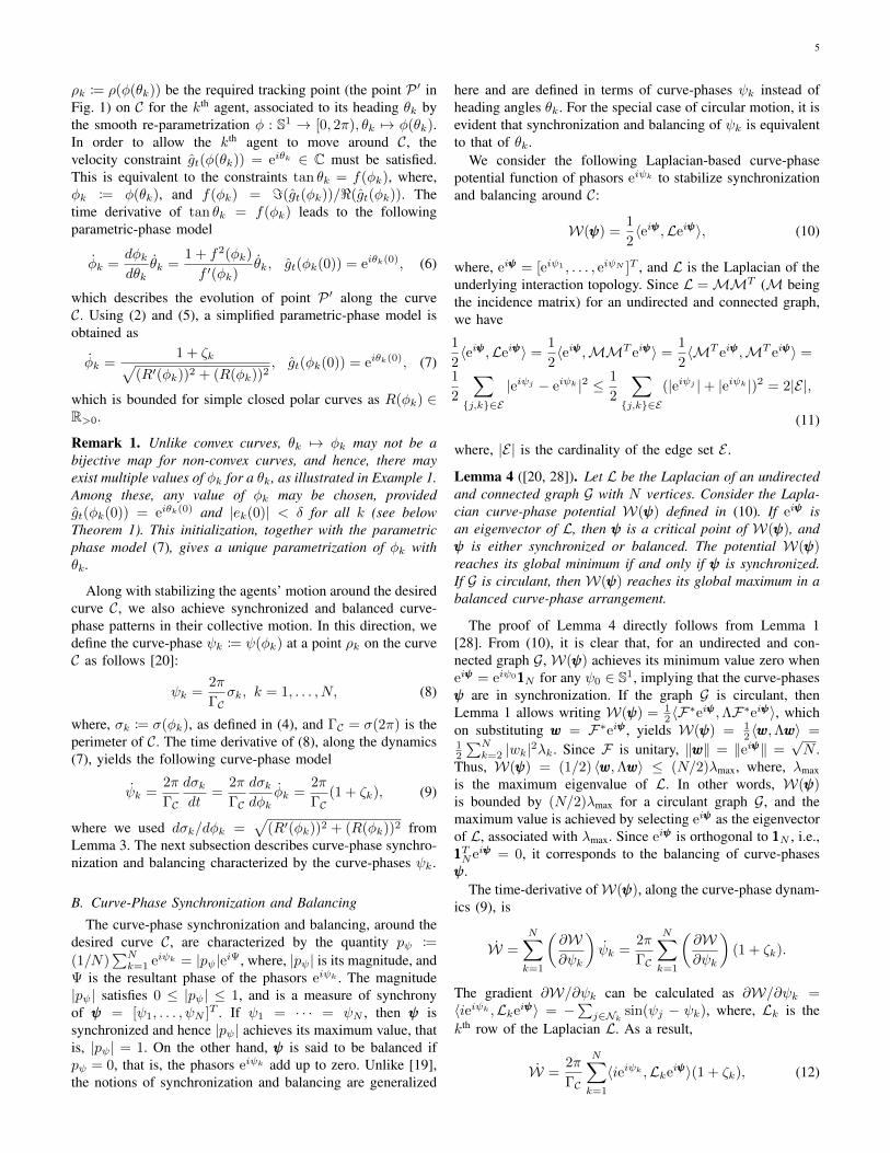
Our first goal is to allow the agents to move around the de-sired curve, characterized by a family of simple closed curvesexpressed in polar form. The problem is shown in Fig. 1, wherethe kth agent is trying to move along the curve C, centeredat the desired location cd. Consider that C is parameterizedby φ with respect to its center cd, and is represented by themap ρ : [0, 2π) → C, φ 7→ ρ(φ). The unit tangent to C atthe point ρ(φ) is gt(φ) = (1/|dρ/dφ|)(dρ/dφ) = eiµ ∈ C,where µ = arg(gt). By rotating eiµ by an angle π/2 radiansin the clockwise direction, we get the exterior unit normalgn(φ) = −ieiµ ∈ C (see Fig. 1). The arc length along thecurve at the point ρ(φ) is σ : [0, 2π)→ R≥0, φ 7→ σ(φ), andis given by
σ(φ) =
∫ φ
0
∣∣∣∣ dρdφ∣∣∣∣ dφ. (4)
The curvature κ : [0, 2π) → R, φ 7→ κ(φ) at the point ρ(φ)on the curve is κ(φ) = dµ/dσ = (dµ/dφ)(dφ/dσ), whichusing (4), gives κ(φ) = (1/|dρ/dφ|)(dµ/dφ). The sign ofκ(φ) is determined by the sense of rotation around C; if thecurve is turning anticlockwise (resp., clockwise) at φ, κ(φ) >

4
-5 0 5
x = R(φ) cosφ
-2
0
2
4
6
y=
R(φ)sinφ
(a) Convex limacon
-10 0 10
x = R(φ) cosφ
-10
-5
0
5
10
y=
R(φ)sinφ
(b) Polar rose
0 2 4 6
φ (rad.)
0.05
0.1
0.15
0.2
0.25
0.3
κ(φ)
(c) κ(φ)−Convex limacon
0 2 4 6
φ (rad.)
-0.5
0
0.5κ(φ)
(d) κ(φ)−Polar rose
Fig. 2. Examples of simple closed curves and their curvature. Convex limaconis plotted for a = 2, b = 4.5, and polar rose (non-convex) for a = 10, b =6, s = 1.
0 (resp., κ(φ) < 0). Note that this convention on κ is givenwith reference to Fig. 1, where the agent is moving in theanticlockwise direction. However, if the agent moves in theclockwise direction, an opposite convention holds as gn(φ)reverses its direction. For simple closed curves, the curvatureis finite and bounded, that is, 0 ≤ |κ(φ)| <∞ for all φ.
Lemma 3 ([26], pg. 40). Consider a family of simpleclosed curves, parameterized by φ, and expressed in po-lar representation as ρ(φ) = R(φ)eiφ ∈ C, R(φ) ∈R>0. Let f(φ), σ(φ) and κ(φ) be the slope of tan-gent, arc-length and curvature, respectively. Then, f(φ) =(R′(φ) sinφ+R(φ) cosφ)/(R′(φ) cosφ−R(φ) sinφ), σ(φ) =∫ φ
0
√(R′(φ))2 + (R(φ))2dφ, and κ(φ) = (2(R′(φ))2 −
R(φ)R′′(φ) + (R(φ))2)/((R′(φ))2 + (R(φ))2)32 , where,
R′(φ) = dR/dφ, and R′′(φ) = d2R/dφ2.
From Lemma 3, one can deduce that
1 + f2(φ)
f ′(φ)=
1
κ(φ)√
(R′(φ))2 + (R(φ))2, (5)
where f ′(φ) = df(φ)/dφ = (2(R′(φ))2 − R(φ)R′′(φ) +(R(φ))2)/(R′(φ) cosφ−R(φ) sinφ)2.
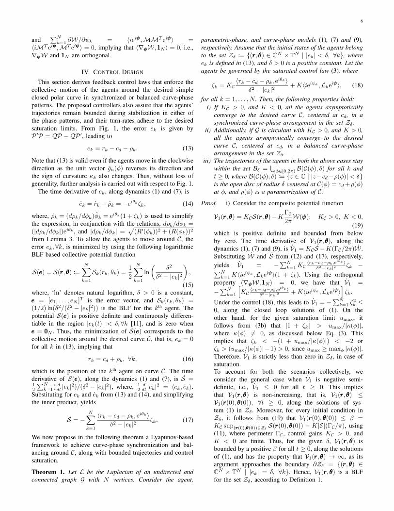
In the following example, we compare convex and non-convex polar curves and illustrate the challenges in designingthe control laws for non-convex curves.
Example 1. Consider a family of simple closed curves,parameterized by φ with respect to the origin, and expressedin polar representation as ρ(φ) = R(φ)eiφ = R(φ) cosφ +iR(φ) sinφ ∈ C, R(φ) ∈ R>0. Depending upon R(φ), weillustrate the following two cases:
Case 1: A convex limacon is an epitrochoid of the formR(φ) = b + a sinφ, b ≥ 2a, where the condition b ≥ 2aensures that the curve is simple and convex. One can ob-tain dρ/dφ =
(a cos 2φ− b sinφ
)+ i
(a sin 2φ+ b cosφ
),
2 4 6 8
µ (rad.)
0
2
4
6
φ(µ)
(rad
.)
(a) φ(µ)−Convex limacon
2 4 6 8
µ (rad.)
0
2
4
6
φ(µ)
(rad
.)
(b) φ(µ)−Polar rose
Fig. 3. The plots for φ(µ) vs µ for the curves in Fig. 2.
which is essentially the tangent vector with slope tanµ =(a sin 2φ+ b cosφ)/(a cos 2φ− b sinφ). From this, it can beobtained that dµ/dφ = κN/κD, where
κN = b2 + 2a2 + 3ab sinφ,
κD = (a cos 2φ− b sinφ)2 + (a sin 2φ+ b cosφ)2,
which on substitution yields the curvature
κ(φ) =dµ
dφ
dφ
dσ=κNκD
dφ
dσ=
κN
(κD)32
,
where we have used the relation dφ/dσ = 1/|dρ/dφ| =1/√κD, in the spirit of (4).
Case 2: A polar rose is of the form R(φ) = s(a +cos(bφ)), a, b, s > 0, where s is a scaling factor and thecondition a, b, s > 0 ensures that the curve is simple andclosed. Similar to the previous case, one can obtain thetangent vector as dρ/dφ = −s(b sin(bφ) cosφ + a sinφ +cos(bφ) sinφ) + is(cos(bφ) cosφ+ a cosφ− b sin(bφ) sinφ),which has slope tanµ = −(cos(bφ) cosφ + a cosφ −b sin(bφ) sinφ)/(b sin(bφ) cosφ + a sinφ + cos(bφ) sinφ). Itcan be shown that dµ/dφ = κN/κD, where
κN = a2 + b2 + a(b2 + 2) cos(bφ) + b2 sin2(bφ) + cos2(bφ)
κD = (b sin(bφ) cosφ+ a sinφ+ cos(bφ) sinφ)2
+ (cos(bφ) cosφ+ a cosφ− b sin(bφ) sinφ)2,
and hence, the curvature is κ(φ) = (1/s)κN/(κD)32 , using
similar steps as above.These curves, along with their curvature, are plotted in
Fig. 2. It is clear that the first curve (Fig. 2(a)) is convex andthe second (Fig. 2(b)) is non-convex, and their curvatures aresmooth and bounded. As the convexity of the curves change,the curvature changes its sign according to the conventionmentioned above. Another important plot is shown in Fig. 3,where φ is plotted against the angle µ of the tangent lineto the curve. It is clear that φ(µ) is a smooth bijective mapfor the convex limacon, while this is not true for the polarrose, which is non-convex. Since the motion around a curverequires an agent to have the tangent velocity vector, non-uniqueness of φ to a tangent poses a challenge in stabilizingthe motion of agents about a general class of simple closedcurves including both convex and non-convex curves. A remedyfor this is presented in Remark 1.
Let us now turn our focus to the kth agent at point Pin Fig. 1, trying to move around the desired curve C. Let
5
ρk := ρ(φ(θk)) be the required tracking point (the point P ′ inFig. 1) on C for the kth agent, associated to its heading θk bythe smooth re-parametrization φ : S1 → [0, 2π), θk 7→ φ(θk).In order to allow the kth agent to move around C, thevelocity constraint gt(φ(θk)) = eiθk ∈ C must be satisfied.This is equivalent to the constraints tan θk = f(φk), where,φk := φ(θk), and f(φk) = =(gt(φk))/<(gt(φk)). Thetime derivative of tan θk = f(φk) leads to the followingparametric-phase model
φk =dφkdθk
θk =1 + f2(φk)
f ′(φk)θk, gt(φk(0)) = eiθk(0), (6)
which describes the evolution of point P ′ along the curveC. Using (2) and (5), a simplified parametric-phase model isobtained as
φk =1 + ζk√
(R′(φk))2 + (R(φk))2, gt(φk(0)) = eiθk(0), (7)
which is bounded for simple closed polar curves as R(φk) ∈R>0.
Remark 1. Unlike convex curves, θk 7→ φk may not be abijective map for non-convex curves, and hence, there mayexist multiple values of φk for a θk, as illustrated in Example 1.Among these, any value of φk may be chosen, providedgt(φk(0)) = eiθk(0) and |ek(0)| < δ for all k (see belowTheorem 1). This initialization, together with the parametricphase model (7), gives a unique parametrization of φk withθk.
Along with stabilizing the agents’ motion around the desiredcurve C, we also achieve synchronized and balanced curve-phase patterns in their collective motion. In this direction, wedefine the curve-phase ψk := ψ(φk) at a point ρk on the curveC as follows [20]:
ψk =2π
ΓCσk, k = 1, . . . , N, (8)
where, σk := σ(φk), as defined in (4), and ΓC = σ(2π) is theperimeter of C. The time derivative of (8), along the dynamics(7), yields the following curve-phase model
ψk =2π
ΓC
dσkdt
=2π
ΓC
dσkdφk
φk =2π
ΓC(1 + ζk), (9)
where we used dσk/dφk =√
(R′(φk))2 + (R(φk))2 fromLemma 3. The next subsection describes curve-phase synchro-nization and balancing characterized by the curve-phases ψk.
B. Curve-Phase Synchronization and Balancing
The curve-phase synchronization and balancing, around thedesired curve C, are characterized by the quantity pψ :=
(1/N)∑Nk=1 eiψk = |pψ|eiΨ, where, |pψ| is its magnitude, and
Ψ is the resultant phase of the phasors eiψk . The magnitude|pψ| satisfies 0 ≤ |pψ| ≤ 1, and is a measure of synchronyof ψψψ = [ψ1, . . . , ψN ]T . If ψ1 = · · · = ψN , then ψψψ issynchronized and hence |pψ| achieves its maximum value, thatis, |pψ| = 1. On the other hand, ψψψ is said to be balanced ifpψ = 0, that is, the phasors eiψk add up to zero. Unlike [19],the notions of synchronization and balancing are generalized
here and are defined in terms of curve-phases ψk instead ofheading angles θk. For the special case of circular motion, it isevident that synchronization and balancing of ψk is equivalentto that of θk.
We consider the following Laplacian-based curve-phasepotential function of phasors eiψk to stabilize synchronizationand balancing around C:
W(ψψψ) =1
2〈eiψψψ,Leiψψψ〉, (10)
where, eiψψψ = [eiψ1 , . . . , eiψN ]T , and L is the Laplacian of theunderlying interaction topology. Since L =MMT (M beingthe incidence matrix) for an undirected and connected graph,we have
1
2〈eiψψψ,Leiψψψ〉 =
1
2〈eiψψψ,MMT eiψψψ〉 =
1
2〈MT eiψψψ,MT eiψψψ〉 =
1
2
∑j,k∈E
|eiψj − eiψk |2 ≤ 1
2
∑j,k∈E
(|eiψj |+ |eiψk |)2 = 2|E|,
(11)
where, |E| is the cardinality of the edge set E .
Lemma 4 ([20, 28]). Let L be the Laplacian of an undirectedand connected graph G with N vertices. Consider the Lapla-cian curve-phase potential W(ψψψ) defined in (10). If eiψψψ isan eigenvector of L, then ψψψ is a critical point of W(ψψψ), andψψψ is either synchronized or balanced. The potential W(ψψψ)reaches its global minimum if and only if ψψψ is synchronized.If G is circulant, then W(ψψψ) reaches its global maximum in abalanced curve-phase arrangement.
The proof of Lemma 4 directly follows from Lemma 1[28]. From (10), it is clear that, for an undirected and con-nected graph G,W(ψψψ) achieves its minimum value zero wheneiψψψ = eiψ0111N for any ψ0 ∈ S1, implying that the curve-phasesψψψ are in synchronization. If the graph G is circulant, thenLemma 1 allows writing W(ψψψ) = 1
2 〈F∗eiψψψ,ΛF∗eiψψψ〉, which
on substituting www = F∗eiψψψ , yields W(ψψψ) = 12 〈www,Λwww〉 =
12
∑Nk=2 |wk|2λk. Since F is unitary, ‖www‖ = ‖eiψψψ‖ =
√N .
Thus, W(ψψψ) = (1/2) 〈www,Λwww〉 ≤ (N/2)λmax, where, λmaxis the maximum eigenvalue of L. In other words, W(ψψψ)is bounded by (N/2)λmax for a circulant graph G, and themaximum value is achieved by selecting eiψψψ as the eigenvectorof L, associated with λmax. Since eiψψψ is orthogonal to 111N , i.e.,111TNeiψψψ = 0, it corresponds to the balancing of curve-phasesψψψ.
The time-derivative ofW(ψψψ), along the curve-phase dynam-ics (9), is
W =
N∑k=1
(∂W∂ψk
)ψk =
2π
ΓC
N∑k=1
(∂W∂ψk
)(1 + ζk).
The gradient ∂W/∂ψk can be calculated as ∂W/∂ψk =〈ieiψk ,Lkeiψψψ〉 = −
∑j∈Nk sin(ψj − ψk), where, Lk is the
kth row of the Laplacian L. As a result,
W =2π
ΓC
N∑k=1
〈ieiψk ,Lkeiψψψ〉(1 + ζk), (12)
6
and∑Nk=1 ∂W/∂ψk = 〈ieiψψψ,MMT eiψψψ〉 =
〈iMT eiψψψ,MT eiψψψ〉 = 0, implying that 〈∇ψψψW,111N 〉 = 0, i.e.,∇ψψψW and 111N are orthogonal.
IV. CONTROL DESIGN
This section derives feedback control laws that enforce thecollective motion of the agents around the desired simpleclosed polar curve in synchronized or balanced curve-phasepatterns. The proposed controllers also assure that the agents’trajectories remain bounded during stabilization in either ofthe phase patterns, and their turn-rates adhere to the desiredsaturation limits. From Fig. 1, the error ek is given byP ′P = QP −QP ′, leading to
ek = rk − cd − ρk. (13)
Note that (13) is valid even if the agents move in the clockwisedirection as the unit vector gn(φ) reverses its direction andthe sign of curvature κk also changes. Thus, without loss ofgenerality, further analysis is carried out with respect to Fig. 1.
The time derivative of ek, along dynamics (1) and (7), is
ek = rk − ρk = −eiθkζk, (14)
where, ρk = (dρk/dφk)φk = eiθk(1 + ζk) is used to simplifythe expression, in conjunction with the relations, dρk/dφk =(|dρk/dφk|)eiθk , and |dρk/dφk| =
√(R′(φk))2 + (R(φk))2
from Lemma 3. To allow the agents to move around C, theerror ek,∀k, is minimized by using the following logarithmicBLF-based collective potential function
S(eee) = S(rrr,θθθ) :=
N∑k=1
Sk(rk, θk) =1
2
N∑k=1
ln
(δ2
δ2 − |ek|2
),
(15)where, ‘ln’ denotes natural logarithm, δ > 0 is a constant,eee = [e1, . . . , eN ]T is the error vector, and Sk(rk, θk) =(1/2) ln(δ2/(δ2 − |ek|2)) is the BLF for the kth agent. Thepotential S(eee) is positive definite and continuously differen-tiable in the region |ek(t)| < δ,∀k [11], and is zero wheneee = 000N . Thus, the minimization of S(eee) corresponds to thecollective motion around the desired curve C, that is, ek = 0for all k in (13), implying that
rk = cd + ρk, ∀k, (16)
which is the position of the kth agent on curve C. The timederivative of S(eee), along the dynamics (1) and (7), is S =12
∑Nk=1( ddt |ek|
2)/(δ2 − |ek|2), where, 12ddt |ek|
2 = 〈ek, ek〉.Substituting for ek and ek from (13) and (14), and simplifyingthe inner product, yields
S = −N∑k=1
〈rk − cd − ρk, eiθk〉δ2 − |ek|2
ζk. (17)
We now propose in the following theorem a Lyapunov-basedframework to achieve curve-phase synchronization and bal-ancing around C, along with bounded trajectories and controlsaturation.
Theorem 1. Let L be the Laplacian of an undirected andconnected graph G with N vertices. Consider the agent,
parametric-phase, and curve-phase models (1), (7) and (9),respectively. Assume that the initial states of the agents belongto the set Zδ := (rrr,θθθ) ∈ CN × TN | |ek| < δ, ∀k, whereek is defined in (13), and δ > 0 is a positive constant. Let theagents be governed by the saturated control law (3), where
ζk = KC〈rk − cd − ρk, eiθk〉
δ2 − |ek|2+K〈ieiψk ,Lkeiψψψ〉, (18)
for all k = 1, . . . , N . Then, the following properties hold:i) If KC > 0, and K < 0, all the agents asymptotically
converge to the desired curve C, centered at cd, in asynchronized curve-phase arrangement in the set Zδ .
ii) Additionally, if G is circulant with KC > 0, and K > 0,all the agents asymptotically converge to the desiredcurve C, centered at cd, in a balanced curve-phasearrangement in the set Zδ .
iii) The trajectories of the agents in both the above cases staywithin the set Bδ =
⋃φ∈[0,2π) B(C(φ), δ) for all k and
t ≥ 0, where B(C(φ), δ) := z ∈ C | |z−cd−ρ(φ)| < δis the open disc of radius δ centered at C(φ) = cd+ρ(φ)at φ, and ρ(φ) is a parametrization of C.
Proof. i) Consider the composite potential function
V1(rrr,θθθ) = KCS(rrr,θθθ)−K ΓC2πW(ψψψ); KC > 0, K < 0,
(19)which is positive definite and bounded from belowby zero. The time derivative of V1(rrr,θθθ), along thedynamics (1), (7) and (9), is V1 = KCS −K(ΓC/2π)W .Substituting W and S from (12) and (17), respectively,yields V1 = −
∑Nk=1KC
〈rk−cd−ρk,eiθk 〉δ2−|ek|2 ζk −∑N
k=1K〈ieiψk ,Lkeiψψψ〉(1 + ζk). Using the orthogonalproperty 〈∇ψψψW,111N 〉 = 0, we have that V1 =
−∑Nk=1
[KC〈rk−cd−ρk,eiθk 〉
δ2−|ek|2 +K〈ieiψk ,Lkeiψψψ〉]ζk.
Under the control (18), this leads to V1 = −∑Nk=1 ζ
2k ≤
0, along the closed loop solutions of (1). On theother hand, for the given saturation limit umax, itfollows from (3b) that |1 + ζk| > umax/|κ(φ)|,where κ(φ) 6= 0, as discussed below Eq. (3). Thisimplies that ζk < −(1 + umax/|κ(φ)|) < −2 orζk > (umax/|κ(φ)|−1) > 0, since umax ≥ maxφ |κ(φ)|.Therefore, V1 is strictly less than zero in Zδ , in case ofsaturation.To account for both the scenarios collectively, weconsider the general case when V1 is negative semi-definite, i.e., V1 ≤ 0 for all t ≥ 0. This impliesthat V1(rrr,θθθ) is non-increasing, that is, V1(rrr,θθθ) ≤V1(rrr(0), θθθ(0)), ∀t ≥ 0, along the solutions of sys-tem (1) in Zδ . Moreover, for every initial condition inZδ , it follows from (19) that V1(rrr(0), θθθ(0)) ≤ β =KC sup(rrr(0),θθθ(0))∈Zδ S(rrr(0), θθθ(0)) − K|E|(ΓC/π), using(11), where perimeter ΓC , control gains KC > 0, andK < 0 are finite. Thus, for the given δ, V1(rrr,θθθ) isbounded by a positive β for all t ≥ 0, along the solutionsof (1), and has the property that V1(rrr,θθθ) → ∞, as itsargument approaches the boundary ∂Zδ = (rrr,θθθ) ∈CN × TN | |ek| = δ, ∀k. Hence, V1(rrr,θθθ) is a BLFfor the set Zδ , according to Definition 1.

7
To prove convergence to the desired curve C, note that theset Ωβ = (rrr,θθθ) ∈ Zδ | V1(rrr,θθθ) ≤ β ⊂ Zδ is compactand positively invariant, since V1(rrr,θθθ) is positive definiteand continuously differentiable, and V1 ≤ 0, alongthe solutions of (1), in Zδ . Therefore, it follows fromLaSalle’s invariance principle [29] that all the solutionsof system dynamics (1), under control (18), converge tothe largest invariant set ∆s
C , contained in the set ∆ ⊂ Ωβ ,where V1 = 0. Thus,
∆ = (rrr,θθθ) ∈ Zδ | ζk = 0,∀k, (20)
which implies using (2) that uk = κ(φ),∀kin ∆. Further, it follows from (18) thatKC〈rk−cd−ρk,eiθk 〉
δ2−|ek|2 = −K〈ieiψk ,Lkeiψψψ〉,∀k in ∆,which upon taking time-derivative on both the sides,yields KC ddt
(〈rk−cd−ρk,eiθk 〉
δ2−|ek|2
)= −K d
dt
(∂W∂ψk
), where
ddt
(∂W∂ψk
)= d
dt 〈ieiψk ,Lkeiψψψ〉 = 〈 ddt (ie
iψk),Lkeiψψψ〉 +
〈ieiψk , ddtLkeiψψψ〉 = 2πΓC
(〈−eiψk ,Lkeiψψψ〉
+〈ieiψk , iLkeiψψψ〉)
= 0. Consequently, for allpoints in ∆s
C ⊂ ∆, we have ddt〈rk−cd−ρk,eiθk 〉
δ2−|ek|2 =
0 =⇒ [(δ2 − |ek|2) ddt 〈rk − cd − ρk, eiθk〉 −
〈rk − cd − ρk, eiθk〉 ddt (δ2 − |ek|2)] = 0. From (17),
it is straightforward to see that ddt (δ
2 − |ek|2) = 0 inthe set ∆s
C . Thus, the previous expression reduces toddt 〈rk − cd − ρk, e
iθk〉 = 0 =⇒ 〈rk−ρk, eiθk〉+κk〈rk−cd − ρk, ieiθk〉 = 0 =⇒ 〈rk − cd − ρk, ieiθk〉 = 0, asrk−ρk = 0 in ∆s
C (see (14)). For 〈rk−cd−ρk, ieiθk〉 = 0to hold, it is necessary that rk = cd + ρk (or ek ⊥ ieiθk
in ∆sC), which is the position of the kth agent moving
around the curve C centered at cd (see (16)). Thus,every trajectory of (1), under control (18), approaches∆sC as t → ∞, i.e., all the agents asymptotically
converge to the desired curve C with center cd inZδ . Alternatively, |ek| → 0 as t → ∞ and hence,S(eee) achieves its minimum if |ek(0)| < δ, ∀k, whichfollows from Lemma 2, as each term Sk(rk, θk) ofS(rrr,θθθ) =
∑Nk=1 Sk(rk, θk) is bounded and approaches
zero.Since V1(rrr,θθθ) = W(ψψψ) in ∆s
C , we conclude that theagents reach an equilibrium with the asymptotic curve-phase arrangements in the critical set of W(ψψψ). SinceV1 ≤ 0, W(ψψψ) also approaches zero, and hence, itfollows from Lemma 4 that the agents are in curve-phasesynchronization around the desired curve C.
ii) To prove this statement, let us consider the potentialfunction
V2(rrr,θθθ) = KCS(rrr,θθθ) +KΓC2π
(N
2λmax −W(ψψψ)
),
(21)with KC > 0,K > 0, which is a valid candidate as0 ≤ W(ψψψ) ≤ (N/2)λmax for an undirected and connectedcirculant graph. The time derivative of V2(rrr,θθθ) alongdynamics (1), (7) and (9), under control (18), resultsin V2 = −
∑Nk=1 ζ
2k = V1 ≤ 0. Thus, the rest of
the proof follows the same steps as given for K < 0.However, in this case, let ∆b
C be the largest invariant
set in ∆ (defined in (20)), which every trajectory of (1)approaches as t → ∞. Following the above analysis,it can be concluded that all the agents asymptoticallyconverge to the desired curve C with center cd in Zδ .Moreover, (N/2)λmax − W(ψψψ) also approaches zero inZδ , as V2 ≤ 0. Since the graph G is circulant, itfollows from Lemma 4 that the agents are in curve-phasebalancing around the desired curve C in Zδ .
iii) Since V1 = V2 ≤ 0 in Zδ , S(eee)(
=∑Nk=1 Sk
)re-
mains bounded. Consequently, for all k = 1, . . . , N ,|ek(φ(t))| < δ, ∀t ≥ 0, according to Lemma 2. Sub-stituting for ek from (13), |ek(φ(t))| < δ =⇒ |rk −cd − ρ(φ)| < δ, ∀k, and ∀φ ∈ [0, 2π). This, in turn,implies that the trajectories of the agents stay within theset Bδ =
⋃φ∈[0,2π) B(C(φ), δ) for all k and t ≥ 0 in both
synchronized and balanced curve-phase arrangements,where B(C(φ), δ) := z ∈ C | |z − cd − ρ(φ)| < δis the open disc of radius δ and center C(φ) = cd + ρ(φ)at φ. Since the result follows for all k, the subscript kis excluded from φ associated to the kth agent, and isdirectly related in terms of its parametrization ρ(φ).
Remark 2. In (18), one may infer that ζk becomes un-bounded whenever |ek| = δ, due to the presence of theterm (δ2 − |ek|2) in the denominator. However, it has beenestablished in Theorem 1 that, in the closed loop, the errorsignal |ek| < δ,∀t ≥ 0, thereby ζk, and hence, uk alwaysremains finite for any solution trajectory. Further, note thatζk may assume any (large/small) value, depending upon thevariables in (18). However, the actual applied control uk in(1) is always bounded as per Eq. (3).
From the preceding discussion, one can observe that, bylimiting the magnitude of the error variables |ek|, the agents’trajectories rk remain bounded within the set Bδ , while thereis no restriction on the heading angles θk of the agents andthese act as the free variables, in accordance with Lemma 2.
In general, it is hard to characterize the explicit nature ofthe boundary ∂Bδ of Bδ in Theorem 1. However, the followingassumption on δ allows us to do so, as discussed in Corollary 1below.
Assumption 1. There exists a constant δ > 0 such that, forevery ε ∈ (0, δ], cd+ρ(φ)±εgn(φ) 6∈ C, φ ∈ [0, 2π). Moreover,for φ1, φ2 ∈ [0, 2π), φ1 6= φ2, it holds that cd + ρ(φ1) +εgn(φ1) 6= cd + ρ(φ2) + εgn(φ2) and cd + ρ(φ1)− εgn(φ1) 6=cd + ρ(φ2)− εgn(φ2).
This assumption essentially ensures that there exists a δ suchthat the locus of the points cd+ρ(φ)±δgn(φ), φ ∈ [0, 2π) formsimple closed curves. Moreover, these curves do not intersectC, if δ is measured along the unit vectors ±gn(φ). Clearly,cd+ρ(φ)− εgn(φ) ∈ int(C), and cd+ρ(φ) + εgn(φ) ∈ ext(C)for each φ ∈ [0, 2π) with respect to Fig. 1. In other words,Assumption 1 proposes certain requirements on C, dependingupon δ. So far as the practical applications are concerned, thisis a mild assumption as discussed later in the paper.

8
cd
CC(φ)
ν+
ν−
δ
δ
B(C(φ), δ)
ρ(φ)
∂B+δ
∂B−δ
Bδ
δ
δ
δ
δ
gn(φ)
Fig. 4. Illustration of the boundary ∂B of the set B, mentioned in Corollary 1.
Corollary 1. Under the conditions in Theorem 1, if addition-ally, Assumption 1 holds, then ∂Bδ = ∂B+
δ ∪ ∂B−δ , where
∂B+δ =
⋃φ∈[0,2π)z ∈ C | z − cd = ρ(φ) + δgn(φ), ∂B−δ =⋃
φ∈[0,2π)z ∈ C | z − cd = ρ(φ) − δgn(φ), and gn(φ) isthe exterior unit normal vector to curve C at φ, as shown inFig. 1.
Proof. Let B(C(φ), δ) := z ∈ C | |z−cd−ρ(φ)| ≤ δ be theclosed disc of radius δ and center C(φ) = cd + ρ(φ) at φ. Forν ∈ B(C(φ), δ), let |projgn(φ)(ν − C(φ))| = |〈ν − C(φ), gn〉|be the absolute value of the projection of ν−C(φ) on gn(φ) atC(φ). Clearly, maxν |projgn(φ)(ν − C(φ))| occurs when 〈ν −C(φ), gn(φ)〉 = ±δ, that is, along the normal vectors to C atφ. This implies that the points ν+ = C(φ)+δgn(φ) and ν− =C(φ)− δgn(φ) are the two farthest points in B(C(φ), δ) fromthe curve C at φ, along exterior and interior normal vectors,respectively (See Fig. 4). Thus, for φ ∈ [0, 2π), the locus ofthe points ν+ and ν− define two boundaries ∂B+
δ and ∂B−δ ,respectively, as mentioned in the statement of Corollary 1. Asa result, ∂Bδ = ∂B+
δ ∪ ∂B−δ , proving our claim.
Remark 3. It is to be noted that Assumption 1 is adapted toexplicitly describe the boundary ∂Bδ of Bδ . However, it is notnecessary and allows any δ > 0, as far as the applicabilityof (18) is concerned. For instance, in the special case of acircle with radius R > 0, ∂Bδ = z ∈ C | |z − cd| = R+ δif δ > R, and ∂Bδ = z ∈ C | |z − cd| = R − δ ∪ z ∈C | |z − cd| = R+ δ if δ < R [19].
Additionally, the following theorem relates perimeters andareas of the regions enclosed by ∂Bδ and curve C, underAssumption 1.
Theorem 2. Let ΓC ,Γ∂Bδ be the respective perimeters ofC and ∂Bδ , and AC ,A∂Bδ the areas enclosed by them inCorollary 1. Then, it holds that Γ∂Bδ = 2ΓC ,A∂Bδ = 2δΓC .
Before proving Theorem 2, we state the following prelimi-nary definition and result from [26, 27].
Definition 2 (Orientation of a Planar Curve [26], pg. 62). Asimple plane closed curve α : [a, b]→ C is called positively-oriented if, for each t ∈ [a, b], iearg(α) points into int(α) inthe sense that there exists δ such that α(t) + isearg(α) lies inint(α) for all s ∈ (0, δ). Otherwise, α is negatively-oriented,in which case iearg(α) points towards ext(α) for all t ∈ [a, b].
Theorem 3 (Hopf’s Umlaufsatz [27], pg. 57). Let α : [a, b]→R2 be a simple closed plane curve with curvature function κ.
Then, its total signed curvature,∫ baκ(t)dt = ±2πI , where I
is referred to as rotation index, and is equal to +1(resp.,−1)for positively-oriented (resp., negatively-oriented) curves.
We are now ready to prove Theorem 2.
Proof. Analogous to the notations in Theorem 2, denote byΓ∂B+
δand Γ∂B−δ
, the perimeters of the boundaries ∂B+δ and
∂B−δ , defined in Corollary 1, and by A∂B+δ
and A∂B−δ , theareas enclosed by them, respectively. Let dµ be the argumentof tangential vector to a differential arc-length dΓC of thecurve C. Considering two adjacent normals to C at the endpoints of dΓC and neglecting higher order terms, one can writedΓ∂B+
δ= dΓC + δdµ; dΓ∂B−δ
= dΓC − δdµ, and d(A∂B+δ−
AC) = 12δ(dΓC + dΓ∂B+
δ) = 1
2δ(2dΓC + δdµ); d(AC −A∂B−δ ) = 1
2δ(dΓC + dΓ∂B−δ) = 1
2δ(2dΓC − δdµ). The termdµ can be written in terms of dφ as dµ = κ(φ)|dρ/dφ|dφ(Subsection III-A). The quantity κT =
∫ 2π
0κ(φ)|dρ/dφ|dφ
is unchanged by re-parametrization [[26], pg. 78]. Thus,using arc-length re-parameterization, we have that κT =∫ ΓC
0κ(σ)|dρ/dσ|dσ =
∫ ΓC0
κ(σ)dσ = 2πI , using Hopf’sUmlaufsatz in Theorem 3, and |dρ/dσ| = 1, according to(4). Under Assumption 1, one can note that C, ∂B+
δ and ∂B−δare positively-oriented simple closed plane curves with respectto Fig. 1, and hence, rotation index I = +1. Using this fact,while integrating previous expressions for a complete circuit,yields Γ∂B+
δ= ΓC + 2πδ; Γ∂B−δ
= ΓC − 2πδ, and A∂B+δ
=
AC + δΓC + πδ2;A∂B−δ = AC − δΓC + πδ2 =⇒ Γ∂Bδ =Γ∂B+
δ+ Γ∂B−δ
= 2ΓC , and A∂Bδ = A∂B+δ− A∂B−δ = 2δΓC ,
as claimed.
Remark 4. The relations in Theorem 2 can also be written interms of area AC (resp., global maximum curvature κmax =maxφ |κ(φ)|) of curve C using the isoperimetric inequalityΓ2C ≥ 4πAC (resp., ΓC ≥ 2π/κmax) for a simple closed plane
curve C, where equality holds if and only if C is a circle [[26],pg. 81, & 98].
In several practical applications, we would often like torestrict the motion of the vehicles in a workspace within theouter boundary. For any convex curve C, the exterior normalsnever intersect irrespective of any δ, and hence, the ideas inTheorem 2 are applicable if one is interested to know theperimeter and area enclosed by the outer boundary.
V. BOUNDS ON VARIOUS SIGNALS
This section obtains bounds on various intermediate signalsbased on Theorem 1. We begin by stating the followingtheorem:
Theorem 4 (Curve-Phase Synchronization). Let L be theLaplacian of an undirected and connected graph G withN vertices. Consider the closed-loop system (1), under thesaturated control law (3) with ζk given by (18), where KC > 0,and K < 0 for all k. Assume that the initial states of theagents belong to the set Zδ , as defined in Theorem 1. Then,the following properties hold:

9
i) The absolute value of ek, and rk, for all k, are boundedby
|ek| = |rk − cd − ρ(φ)| ≤ δ√
1− e−(
2V1(0)KC
).
ii) The squared summation of the absolute value of therelative curve-phasors eiψj−eiψk belongs to the compactset∑j,k∈E
|eiψj−eiψk |2 ∈[0,min
−(
4πV1(0)
KΓC
), 4|E|
],
where, V1(0) = V1(rrr(0), θθθ(0)), and |E| is the cardinalityof the edge set E of the graph G, respectively.
Proof. i) Following Theorem 1, since V1(rrr(t), θθθ(t)) ≤V1(0),∀t ≥ 0, in Zδ , it follows from (19)that KC
2
∑Nk=1 ln
(δ2
δ2−|ek(t)|2
)≤ V1(0) =⇒
ln(
δ2
δ2−|ek(t)|2
)≤ 2V1(0)
KC, ∀k, and ∀t ≥ 0,
in Zδ . Taking exponential on both side, yieldsδ2/(δ2 − |ek(t)|2) ≤ e
2V1(0)KC . It has been established
in Theorem 1 that |ek(t)| < δ, ∀k, and ∀t, implyingthat δ2 − |ek(t)|2 > 0,∀k, and ∀t. Thus, we ob-
tain δ2 ≤ e2V1(0)KC (δ2 − |ek(t)|2) =⇒ |ek(t)| ≤
δ√
1− e−(2V1(0)/KC),∀k and ∀t ≥ 0. Further, substi-tuting for ek from (13), it implies that |rk(t) − cd −ρ(φ(t))| ≤ δ
√1− e−(2V1(0)/KC),∀k and ∀t ≥ 0.
ii) A similar argument as above for the second term onRHS in (19), results in W(ψψψ) ≤ − 2πV1(0)
KΓC. Sub-
stituting for W(ψψψ) from (10), one can write that〈eiψψψ,Leiψψψ〉 ≤ − 4πV1(0)
KΓC. However, it follows from (11)
that 〈eiψψψ,Leiψψψ〉 =∑j,k∈E |eiψj − eiψk |2 ≤ 22|E|,
for any undirected and connected graph G. Thus, therequired bounds on
∑j,k∈E |eiψj − eiψk |2, as given in
the theorem, is obtained.
Theorem 5 (Curve-Phase Balancing). Let L be the Laplacianof an undirected and connected circulant graph G with Nvertices. Consider the closed-loop system (1), under the sat-urated control law (3) with ζk given by (18), where KC > 0,and K > 0 for all k. Assume that the initial states of theagents belong to the set Zδ , as defined in Theorem 1. Then,the following properties hold:
i) The absolute value of ek, and rk, for all k, are boundedby
|ek| = |rk − cd − ρ(φ)| ≤ δ√
1− e−(
2V2(0)KC
).
ii) The squared summation of the absolute value of eiψj −eiψk belongs to the compact set∑
j,k∈E
|eiψj − eiψk |2 ∈ J ,
where,
J =
[max
0,
(Nλmax −
(4πV2(0)
KΓC
)), Nλmax
],
1
2
3
45
6
7
(a) Topology
4
4
4
4
4
4
4
−1
−1
−1
−1
−1
−1
−1
−1
−1
−1
−1
−1
−1
−1
−1
−1
−1
−1
−1 −1
−1
−1
−1
−1 −1
−1
−1
−1
0
0
0
0
0
0
0
0
0
0
0
00
0
(b) Laplacian L
Fig. 5. Interaction topology and associated Laplacian for N = 7 agents.
and V2(0) = V2(rrr(0), θθθ(0)), and |E|, is as defined inTheorem 4.
Proof. For any undirected and connected circulant graph(N/2)λmax ≤ 2|E|, with equality if and only if the circu-lant graph G forms a ring topology (that is, the minimallyconnected circulant graph). Thus, the bound in case ii) ofTheorem 5 is different than that from Theorem 4. The restof the proof follows along the similar steps as in Theorem 4,and hence omitted.
Remark 5. Note that Corollary 1 and Theorem 2can be written equivalently, individually for curve-phase synchronization and balancing, by replacingδ with δs = δ
√1− e−(2V1(0)/KC) < δ and
δb = δ√
1− e−(2V2(0)/KC) < δ, derived using the tighterbound |rk − cd − ρ(φ)| ≤ δ
√1− e−(2V1(0)/KC) and
|rk − cd − ρ(φ)| ≤ δ√
1− e−(2V2(0)/KC), on the trajectoriesof the agents in Theorem 4 and Theorem 5, respectively.
The prerequisite of our approach is that the agents’ initialconditions must satisfy |ek(0)| < δ for all k. We characterizethe feasible initial conditions in the following theorem.
Theorem 6. The condition |ek(0)| < δ is satisfied for all k,if the initial conditions (that is, initial positions rk(0) andheading angles θk(0)) of the agents in (1) belong to the setBδ , where, ek and Bδ are defined in (13) and Theorem 1,respectively.
Proof. The proof directly follows from Theorem 1 and Corol-lary 1. Note that there exists at least one setting of the initialconditions such that |ek(0)| < δ is satisfied for all k, asθk(0) ∈ S1 are free states.
VI. SIMULATION RESULTS
Consider seven agents (N = 7) with an interaction topologygiven by a circulant graph G in Fig. 5. Let us stabilize theagents around the polar-rose curve, as discussed in Example 1,with parameters a = 10, b = 6, s = 5, and center atcd = (0, 0). Assume δ = 12. The initial positions and headingangles of the agents are randomly chosen to satisfy |ek(0)| < δfor all k = 1, . . . , 7, according to Theorem 6, and arexxx(0) = [32.6, 8.1,−50.2,−6.7, 64.4,−46.1,−60.6]T , yyy(0) =[18.7,−42.5, 21.2,−48.2,−7.0,−9.2,−10.8]T , and θθθ(0) =[127.3, 341.2, 222.6, 18.5, 59.5, 314.3, 271.7]T . Sinceδ < minφ|1/κ(φ)| = 12.87, one can easily observe thatAssumption 1 holds for this curve, and hence, there exist innerand outer boundaries ∂B−δ and ∂B+
δ , as defined in Corollary 1.

10
-50 0 50
X (m)
-50
0
50Y
(m)
∂B−
δ
∂B+δ
(a) Synchronization
-50 0 50
X (m)
-50
0
50
Y(m
)
∂B−
δ
∂B+δ
(b) Balancing
0 500 1000 1500 2000
time (sec.)
0
2
4
6
8
10
12
|ek|
δs ≈ δ
(c) Errors−synchronization
0 500 1000 1500 2000
time (sec.)
0
2
4
6
8
10
12|e
k|
δb ≈ δ
(d) Errors−balancing
Fig. 6. Agents’ trajectories and the absolute errors |ek| with time.
• Fig. 6 shows the agents’ trajectories and errors ek for bothcurve-phase synchronization and balancing. The resultsare obtained under control law (18) with gains KC = 2.5and K = −0.1 (resp., 0.2) for synchronization (resp.,balancing). It is clearly seen that the agents achievesynchronization and balancing, and their trajectories staywithin the set Bδ , bounded by ∂B−δ and ∂B+
δ . Moreover,the absolute value of errors |ek| for all k = 1, . . . , 7, arebounded by δs ≈ δ (resp., δb ≈ δ) for synchronization(resp., balancing) and approaches zero, as desired. Froman application point of view, one can consider that theagents are moving in different planes in curve-phasesynchronization [15, 19].
• Control inputs uk in (3) are depicted in Fig. 7 for allk = 1, . . . , 7, where we assumed that the saturation limitis umax = 0.0786 such that umax ≥ maxφ |κ(φ)| = 0.0776in (3). Clearly, |uk| ≤ umax for all k = 1, . . . , 7in both curve-phase synchronization and balancing. Animportant observation in Fig. 7 is that the control inputsuk are also synchronized and phase-shifted in time forsynchronization and balancing, respectively. Further, wealso observe that ζk → 0 (and uk = κ(φ)), ∀ k = 1, . . . , 7in steady state, when the agents converge to the desiredcurve in synchronized and balanced phase patterns.
• Fig. 8 sketches the magnitude |pψ| of the average curve-phase momentum pψ , the curve-phase potential W(ψψψ),and the quantity H(ψψψ) =
∑j,k∈E |eiψj − eiψk |2 for
both curve-phase synchronization and balancing. It canbe seen that |pψ| → 1 and W(ψψψ) → 0 in case ofsynchronization. For balancing, |pψ| → 0 and W(ψψψ) →(N/2)λmax(L) = 21.86 < 2|E| = 26, as discussed inLemma 4 and Theorem 5. Moreover,H(ψψψ) ∈ [0, 30.7] forsynchronization, and H(ψψψ) ∈ [25.1, 43.7] for balancing.These bounds are calculated using Theorems 4 and 5, andare verified in Fig. 8.
0 500 1000 1500 2000
time (sec.)
-0.0
90
0.0
9
uk
-umax
umax
(a) Control−synchronization
0 500 1000 1500 2000
time (sec.)
-0.0
90
0.0
9
uk
-umax
umax
(b) Control−balancing
0 500 1000 1500 2000
time (sec.)
-0.4
-0.2
00.2
0.4
0.6
ζ k
(c) ζk−synchronization
0 500 1000 1500 2000
time (sec.)
-0.6
-0.4
-0.2
00.2
0.4
0.6
ζ k
(d) ζk−balancing
Fig. 7. Control inputs uk in (3) with time.
0 1000 2000
time (sec.)
0.2
0.4
0.6
0.8
1
|pψ|
0
5
10
15
W(ψ
)(a)|pψ |,Wψ−synchronization
0 1000 2000
time (sec.)
0
0.1
0.2
0.3
|pψ|
12
14
16
18
20
22
W(ψ
)
N2 λmax = 21.86
(b) |pψ |,Wψ−balancing
0 500 1000 1500 2000
time (sec.)
0
10
20
30
40
H(ψ
)
(c) H(ψψψ)−synchronization
0 500 1000 1500 2000
time (sec.)
25
30
35
40
45
H(ψ
)
(d) H(ψψψ)−balancing
Fig. 8. Curve-phase characteristics for synchronization and balancing.
• In Fig. 9, we observe that the agent headings θk and curvephases ψk converge in the case of synchronization, as theagents converge to the desired curve. For the balancedphase pattern of N = 7 agents, the curve-phases arespaced apart by 2π
7 radians in the steady state (see Fig.9(d)).
• We have numerically calculated the parameters and ar-eas of the curves and boundaries. It is observed thatΓC = 340.82 (m), and Γ∂B−δ
= ΓC − 2πδ =265.43 (m); Γ∂B+
δ= ΓC + 2πδ = 416.21 (m), satisfying
Theorem 2. The area enclosed by the desired curve, andthe inner and outer boundaries are also calculated nu-

11
0 500 1000 1500 2000
time (sec.)
0
10
20
30
40
50
θk(rad.)
(a) θk−synchronization
0 500 1000 1500 2000
time (sec.)
-10
0
10
20
30
40
50
θk(rad.)
(b) θk−balancing
0 500 1000 1500 2000
time (sec.)
0
10
20
30
40
50
ψk(rad.)
(c) ψk−synchronization
0 500 1000 1500 2000
time (sec.)
0
10
20
30
40
50ψk(rad.)
2π/7
(d) ψk−balancing
Fig. 9. Agents’ heading and curve-phases for synchronization and balancing.
merically and agree with Theorem 2, AC = 7893.3 (m2),A∂B−δ = AC − δΓC + πδ2 ≈ 4255.7 (m2), and A∂B+
δ=
AC + δΓC +πδ2 ≈ 12435.4 (m2). It is straightforward tocheck that Γ∂Bδ = Γ∂B+
δ+ Γ∂B−δ
= 2ΓC = 681.64 (m),and A∂Bδ = A∂B+
δ−A∂B−δ = 2δΓC ≈ 8179.7 (m2). Fur-
thermore, the inequalities Γ2C = 116158.6 > 99189.5 =
4πAC , and ΓC = 340.82 > 80.87 = 2π/κmax, asmentioned in Remark 4, are also verified.
VII. CONCLUSION AND FURTHER REMARKS
Formation patterns of multi-agent systems in curve-phasesynchronization and balancing around a desired simple closedcurve, while considering two practical aspects−bounded tra-jectories and saturated control, were investigated in this paper.The concept of logarithmic BLF was used to derive the controllaws. Using tools from Lyapunov stability theory and LaSalle’sinvariance principle, it was shown that the proposed controllersasymptotically stabilize the desired formation patterns aroundthe desired simple closed polar curve, while the agents’ trajec-tories remain bounded and the turn-rates obey the saturationlimits. The analytical expressions for boundary, perimeter, andarea of the trajectory-constraining set, were obtained undera mild assumption on the safe distance from the desiredcurve. Bounds on several signals of interest were derived andshown to be a function of initial conditions, control gains,and interaction topology among agents. Extensive MATLABsimulations were provided to illustrate the theoretical results.
The issue of collision avoidance among agents is not ad-dressed in this paper. In this work, the control input is realizedthrough turn-rates of the vehicles. However, one will requirea higher level of control efforts to tackle collision avoidance[1, 2, 4]. The incorporation of practical aspects like com-munication time-delays, directed and dynamically changinginteraction topology, external disturbances, etc., constitute an
interesting and indeed a challenging future scope of the work,due to nonlinear nature of the control laws.
ACKNOWLEDGMENTS
The authors would like to gratefully acknowledge Prof.Debasish Ghose for his helpful comments and suggestions.
REFERENCES
[1] D. Panagou, D. M. Stipanovic, and P. G. Voulgaris,“Multi-objective control for multi-agent systems usinglyapunov-like barrier functions,” in 52nd IEEE Confer-ence on Decision and Control. IEEE, 2013, pp. 1478–1483.
[2] D. Panagou, D. M. Stipanovic, and P. G. Voulgaris, “Dis-tributed coordination control for multi-robot networks us-ing lyapunov-like barrier functions,” IEEE Transactionson Automatic Control, vol. 61, no. 3, pp. 617–632, 2015.
[3] P. Glotfelter, J. Cortes, and M. Egerstedt, “Nonsmoothbarrier functions with applications to multi-robot sys-tems,” IEEE control systems letters, vol. 1, no. 2, pp.310–315, 2017.
[4] D. Han and D. Panagou, “Robust multitask formationcontrol via parametric lyapunov-like barrier functions,”IEEE Transactions on Automatic Control, vol. 64, no. 11,pp. 4439–4453, 2019.
[5] C. K. Verginis and D. V. Dimarogonas, “Closed-formbarrier functions for multi-agent ellipsoidal systems withuncertain lagrangian dynamics,” IEEE Control SystemsLetters, vol. 3, no. 3, pp. 727–732, 2019.
[6] U. Lee and M. Mesbahi, “Constrained consensus vialogarithmic barrier functions,” in 2011 50th IEEE con-ference on decision and control and European controlconference. IEEE, 2011, pp. 3608–3613.
[7] M. Z. Romdlony and B. Jayawardhana, “Uniting controllyapunov and control barrier functions,” in 53rd IEEEConference on Decision and Control. IEEE, 2014, pp.2293–2298.
[8] ——, “Stabilization with guaranteed safety using controllyapunov–barrier function,” Automatica, vol. 66, pp. 39–47, 2016.
[9] A. D. Ames, X. Xu, J. W. Grizzle, and P. Tabuada,“Control barrier function based quadratic programs forsafety critical systems,” IEEE Transactions on AutomaticControl, vol. 62, no. 8, pp. 3861–3876, 2016.
[10] A. D. Ames, S. Coogan, M. Egerstedt, G. Notomista,K. Sreenath, and P. Tabuada, “Control barrier functions:Theory and applications,” in 2019 18th European ControlConference (ECC). IEEE, 2019, pp. 3420–3431.
[11] K. P. Tee, S. S. Ge, and E. H. Tay, “Barrier lyapunovfunctions for the control of output-constrained nonlinearsystems,” Automatica, vol. 45, no. 4, pp. 918–927, 2009.
[12] K. P. Tee, B. Ren, and S. S. Ge, “Control of nonlinearsystems with time-varying output constraints,” Automat-ica, vol. 47, no. 11, pp. 2511–2516, 2011.
[13] Z.-L. Tang, K. P. Tee, and W. He, “Tangent barrierlyapunov functions for the control of output-constrained

12
nonlinear systems,” IFAC Proceedings Volumes, vol. 46,no. 20, pp. 449–455, 2013.
[14] W. He, C. Sun, and S. S. Ge, “Top tension control of aflexible marine riser by using integral-barrier lyapunovfunction,” IEEE/ASME Transactions on Mechatronics,vol. 20, no. 2, pp. 497–505, 2014.
[15] N. E. Leonard, D. A. Paley, F. Lekien, R. Sepulchre,D. M. Fratantoni, and R. E. Davis, “Collective motion,sensor networks, and ocean sampling,” Proceedings ofthe IEEE, vol. 95, no. 1, pp. 48–74, 2007.
[16] K. Ovchinnikov, A. Semakova, and A. Matveev, “Coop-erative surveillance of unknown environmental bound-aries by multiple nonholonomic robots,” Robotics andAutonomous Systems, vol. 72, pp. 164–180, 2015.
[17] L. Brinon-Arranz, L. Schenato, and A. Seuret, “Dis-tributed source seeking via a circular formation of agentsunder communication constraints,” IEEE Transactions onControl of Network Systems, vol. 3, no. 2, pp. 104–115,2015.
[18] L. Brinon-Arranz, A. Renzaglia, and L. Schenato, “Mul-tirobot symmetric formations for gradient and hessianestimation with application to source seeking,” IEEETransactions on Robotics, vol. 35, no. 3, pp. 782–789,2019.
[19] A. Jain and D. Ghose, “Trajectory-constrained collectivecircular motion with different phase arrangements,” IEEETransactions on Automatic Control, vol. 65, no. 5, pp.2237–2244, 2019.
[20] D. A. Paley, N. E. Leonard, and R. Sepulchre, “Stabiliza-tion of symmetric formations to motion around convexloops,” Systems & Control Letters, vol. 57, no. 3, pp.209–215, 2008.
[21] Y.-Y. Chen and Y.-P. Tian, “Formation tracking andattitude synchronization control of underactuated shipsalong closed orbits,” International Journal of Robust andNonlinear Control, vol. 25, no. 16, pp. 3023–3044, 2015.
[22] L. Sabattini, C. Secchi, and C. Fantuzzi, “Closed-curvepath tracking for decentralized systems of multiple mo-bile robots,” Journal of Intelligent & Robotic Systems,vol. 71, no. 1, pp. 109–123, 2013.
[23] F. Zhang and N. E. Leonard, “Coordinated patterns ofunit speed particles on a closed curve,” Systems & controlletters, vol. 56, no. 6, pp. 397–407, 2007.
[24] X. Xu, T. Waters, D. Pickem, P. Glotfelter, M. Egerstedt,P. Tabuada, J. W. Grizzle, and A. D. Ames, “Realizingsimultaneous lane keeping and adaptive speed regulationon accessible mobile robot testbeds,” in 2017 IEEE Con-ference on Control Technology and Applications (CCTA).IEEE, 2017, pp. 1769–1775.
[25] P. J. Davis, Circulant matrices. American MathematicalSoc., 2013.
[26] K. Tapp, Differential geometry of curves and surfaces.Springer, 2016.
[27] A. N. Pressley, Elementary differential geometry.Springer Science & Business Media, 2010.
[28] A. Jain and D. Ghose, “Collective circular motion insynchronized and balanced formations with second-orderrotational dynamics,” Communications in Nonlinear Sci-
ence and Numerical Simulation, vol. 54, pp. 156–173,2018.
[29] H. K. Khalil, Nonlinear systems. Prentice hall UpperSaddle River, NJ, 2002, vol. 3.