LAPPEENRANTA UNIVERSITY OF TECHNOLOGY

Faculty of Technology

Master’s Degree Programme in Energy Technology

Synchronous machine vector control system development and

implementation

Supervisors: Olli Pyrhönen, Pasi Peltoniemi

Author: Konstantin Vostrov

Lappeenranta 2016

Abstract

Author: Konstantin Vostrov

Thesis title: Synchronous machine vector control system

development and implementation

Faculty: Department of Electrical Engineering

Major: Industrial Electronics

Year of graduation: 2016

Master’s Thesis: Lappeenranta University of Technology

75 pages, 50 figures, 3 tables, 2 appendixes

Examiners: Prof. Olli Pyrhönen, D.Sc. Pasi Peltoniemi

Keywords: Synchronous motor, Vector control, Field

oriented control, PI-controller, Bechoff,

TwinCAT, Simulink

This Master Thesis describes the vector control system of synchronous motor design and

implementation. Theoretical background part includes basic knowledge about synchronous

machines, their classification and control methods. Further in the thesis basic principles of

Internal Model Control Method (IMC) for tuning PI-controller parameters are described.

Application of the IMC for setting the PI controller parameters in relation to the present paper

method is also presented. The electrical drive system, including vector control system, was

created in Matlab Simulink and PI-controllers parameters were tuned more precisely using

sensitivity function analysis tools, provided by Matlab. In the code processing part of the thesis,

Simulink-based model was converted into Visual Studio TwinCAT XAE environment. Also

some final model and PI-controller parameters tuning, caused by converting, was done. The

generated code was downloaded into FPGA- hardware and PC-based control and tested in the

laboratory in order to operate with a real 12.5 kVA synchronous motor. Laboratory tests and

results are described in respective parts.

Acknowledgements

First and foremost I want to express my gratitude to my family, people who was waiting for

me at home and who worried about me and my studies as well as for themselves. Tatiana, my lovely

mom, who was missing me most of all my relatives, thank you for your patience, support and

encouraging during this period of my life and for the fact that I became who I am.

I want to thank all my friends, both old and newfound during studying in Finland. Without

your support and having leisure time together I would lost my mind during the writing of this work.

I want to express my deepest gratitude to all the people who were directly involved in this

project. My supervisors Prof. Olli Pyrhönen, the person who organized this thesis possible, and

D. Sc. Pasi Peltoniemi - people who are easy to work with and who was always happy to share their

knowledge and experience. I want to ask forgiveness from everybody for my ridiculous and stupid

questions that I was asking you during the time of writing on this thesis.

Special thanks to Electrical Drives laboratory staff and particularly to M.Sc. Teemu Sillanpää

for his invaluable help and titanic work on the preparation and holding of laboratory tests.

Would like to thank all the administrative staff of Electrical Engineering department and LUT

at all. My special thanks to D. Sc. Julia Vauterin-Pyrhönen, the person who was taking care of us,

newcomers in LUT, from the first days of our studying and who can help you to find a solution in

almost any problem situation.

Thanks to the administration of Peter the Great Saint-Petersburg Polytechnic University and

Lappeenranta University of Technology for collaboration and carrying out the double degree

program in Master’s degree.

Finally, would like to thank all the Finnish people for this great experience of the wonderful

life in this country and people who made my stay in Finland and in Lappeenranta comfortable and

enjoyable, thanks to LOAS for providing a nice apartment for all of us (newcomers 2015), thanks

to Aalef and of course Sodexo campus restaurants for a tasty meals all these hard studying months,

thanks to IT department, library, cleaning and other university and maintenance staff who was doing

their job well day by day in order to we, the students, could learn 24 hours a day, fully focusing on

the studies and without any problems could have everything we need for a fruitful productive

educational process.

Lappeenranta, November 2016

List of abbreviations and symbols

a phase shift operator

AC alternating current

DC direct current

DIMC Diagonal Internal Model Control method

DOL direct online start

DTC direct torque control

e decoupling term

EESM electrically excited synchronous machine

f frequency [Hz]

FOC field oriented control

FPGA field-programmable gate array

I electric current [A]

i electric current, instantaneous value i(t) [A]

IMC Internal Model Control method

k phase shift angle between the U-axis and the x-axis

Ki integral coeffitient

Kp proportional koeffitient

L inductance [H]

n rotation speed [1/s]

p number of pole pairs

PI proportional–integral controller

R resistance [Ohm]

SI International System of Units

SM synchronous machine

T torque [N m]

t time [s]

Ti integrator time [s]

tr rise time [s]

U voltage [V], RMS, depiction of phase

u voltage, instantaneous value u(t) [V]

V depiction of phase

W depiction of phase

α bandwidth

δ load angle [rad]

ψ magnetic flux linkage [V s]

ω electrical angular velocity [rad/s], angular frequency [rad/s]

Subscripts

0 zero sequence value

1 primary, initial, input value, stator

2 secondary, transformed, output value, rotor

cc current control

d direct

D direct, for damper winding

e electromagnetic

f field (excitation)

load load

m magnetizing

mech mechanical

q quadrature

Q Quadrature, for damper winding

r reference, rotor

ref reference

s stator

T value responsible for torque control

u depiction of phase

v depiction of phase

w depiction of phase

α alpha axis direction

β beta axis direction

σ flux leakage

ψ magnetic flux linkage

ω angular speed

Superscripts

g rotor reference frame

s stator reference frame

Contents

1. Introduction ......................................................................................................................... 8

1.1. Brief information about different types of machines.......................................................... 8

1.2 Different synchronous machines types ............................................................................. 10

1.3 The design concept of the synchronous machine. ............................................................. 12

Feeding of the field winding. ............................................................................................. 15

1.4 Variable speed motors control.......................................................................................... 16

1.5 Vector control methods .................................................................................................... 18

1.6 Converter technology overview ....................................................................................... 20

2. Drive system modelling and mathematical model description ............................................ 23

2.1. Stator current control ...................................................................................................... 32

2.2. Excitation Current Control .............................................................................................. 33

2.3. Speed Control ................................................................................................................. 35

2.4. Stator Flux Control ......................................................................................................... 40

2.5. Model running ................................................................................................................ 44

3. Hardware description ......................................................................................................... 48

3.1 General structure ............................................................................................................. 48

3.2. Electromechanical part ................................................................................................... 49

3.3. Power converter and its control board ............................................................................. 51

3.4. FPGA ............................................................................................................................. 53

3.5. PC-based Bechoff TwinCAT .......................................................................................... 54

4. Code processing and laboratory tests preparation ............................................................... 55

4.1 General information ......................................................................................................... 55

4.2 Simulink to TwinCAT XAE transferring ......................................................................... 56

4.3 Adjusting the model to real hardware requirements .......................................................... 58

4.4 First test simulation ......................................................................................................... 59

4.5 Second test simulation ..................................................................................................... 61

4.3 Code downloading into hardware ..................................................................................... 63

5. Laboratory tests ..................................................................................................................... 64

5.1 First test run..................................................................................................................... 64

5.2 Second test run ................................................................................................................ 66

6. Test results processing ....................................................................................................... 68

7. Conclusions ....................................................................................................................... 70

8. References ............................................................................................................................ 71

Appendixes ............................................................................................................................... 73

1. Introduction

The purpose of this work is to implement a special electrical drive system for laboratory’s

research needs. The research laboratory of Electrical Engineering Department of Lappeenranta

University of Technology needs to have a vector controlled synchronous machine as a test platform

for electrically exited synchronous machine (EESM) control system testing and developing, where

it could be possible to change control algorithms freely, which is impossible in totally assembled

commercial converters available in the market.

Therefore, the aim is to implement vector control system for a real electrical machine in the

laboratory. The control system was developed and tested using simulation software Matlab

Simulink, which is further implemented for laboratory control electronics. The target prototype is

a 12.5 kVA synchronous motor with electrically excited rotor. The way of implementation is to

use common frequency converter based on semiconductor bridge and tailor made control

electronics.

To reach the mentioned goal, in this project following steps have been done. Drive system

modelling and preliminary control tuning was done in Simulink, code building and final model

tuning was done in Microsoft Visual Studio TwinCAT XAE environment. Control algorithm was

translated into real control electronics, and control system was tested in the real laboratory system.

1.1. Brief information about different types of machines

In present day electrical drives are one key technology in industrial systems. During the 200

years of developing electrical drives [1] several different types of electrical motors have been

developed and exist today (fig. 1.1)

Main focus of this thesis is on synchronous machine and its control. In the following,

synchronous machine will be considered more in detail.

Fig.1.1. Different types of electrical motors

Synchronous machines are often used as a source of electrical AC energy commonly

installed on powerful thermal, hydraulic and nuclear power plants, as well as mobile power stations

and transport units (locomotives, cars, airplanes). The design of the synchronous generator is

mainly determined by the type of drive depending on this distinguished turbo-generators, hydro-

generators and diesel generators. Turbo-generators are driven by steam or gas turbines, hydro -

hydro turbines, diesel generators - the internal combustion engine. Synchronous machines are

widely used as electric motors with an output power of 100 kW and higher to drive pumps,

compressors, fans and other mechanisms operating at a constant speed. They are also used as

synchronous compensators for generating or consuming reactive power in order to improve

Electrical Drives

DC AC

Induction motorsSynchronous

motors

Electrically excited SM

Permanent magnet SM

Synchronous reluctanse SM

Hysteresis motors

Switched reluctance motors

network power factor and voltage regulation. One advantage of synchronous motors in comparison

with induction motors is the higher overloadability. It is important, that the synchronous motor

overload capacity can be increased by automatically adjusting the excitation current, while the

induction motors has not such opportunity.

Moreover, in a real conditions overload capability of asynchronous motors with the sudden

increase of load is reduced due to undervoltage in feeding network and due to increasing slip in

the motor. Short-term use of the overload capacity of the induction motor, when a shock load is

given, is possible only at the expense of speed. Changing the slip can be reduced by a flywheel,

but this increases the cost and complicates its installation operation.

Synchronous machine speed at shock load remains almost unchanged. Synchronous motors

are successfully used in mechanisms with the shock load, for example in steel mills and other

heavy industrial applications. Powerful synchronous motors can produce an output power up to 60

MW and more. The highest power ratings motors for specific applications can produce power up

to 100 MW [2] and higher. In case of using synchronous machine as a generators, its power can

reach several hundreds of MWs [3].

An important advantage of synchronous motors to asynchronous is the ability to use them as

a source of reactive power to maintain the desired level of tension in the load assembly. If the load

is strongly unstable, the synchronous motor must be equipped with automatic excitation controller

for a given load node voltage control and forcing excitation in order to maintain the stability of the

engine [1], [4].

Synchronous electrical machines are profitable at powers upwards from 100 kW, and the

main applications are powerful fans, compressors and other heavy duty units. Drawbacks of there

are constructive complexity, the presence of an external excitation of the rotor winding, the

complexity of start and relatively high cost [5].

1.2 Different synchronous machines types

In general, synchronous machines can be divided into 2 major groups: machines which has

an excitation winding, and non-excited machines. In the following, overview of these two machine

types is given.

Synchronous machines with rotor windings are called either wounded rotor synchronous

machines (WRSM) or electrically exited synchronous machines (EESM). This type of machines

are commonly used both as generators and motor drives. DC-excited motors are usually designed

for using in large-scale application (upward from several hundred watts). These type of

synchronous motors requires direct current supplied to the rotor for excitation. In most cases rotor

supplied through slip rings, but a brushless AC motor technology may also be used. The excitation

current may be supplied from a separate DC source or from a DC generator directly connected to

the motor shaft. By varying the excitation of a synchronous motor, it is possible to operate at

lagging, leading and unity power factor. The excitation alternatives will be described in detail in

the next chapter.

In addition to EESMs there are several types of machines designed to operate without

excitation windings on the rotor. Depending on the characteristics of the electromagnetic system,

non-excited synchronous machines are divided into the following types: motors and generators

with permanent magnets, synchronous reluctance machines and stepping (pulse) engines. These

operate normally without excitation windings on the rotor, which greatly increases their reliability

and simplifying construction.

Permanent magnet synchronous machines are widely used as a micromachines. Nowadays

PM-motors are also used in higher power range industrial applications such as a gearless elevator

motors, in marine propulsion drives, as a hydrogenerators and wind turbine generators.

The automatic devices are widely applying synchronous micromotors with capacity of watts

to several hundred watts. A characteristic feature of these motors is that their speed n2 = n1 is

rigidly connected to the power line frequency f1, so they are used in various devices, where

constant speed is required (in the electric clockworks, the tape drive recording instruments and

film projectors, radio equipment, software devices and so on), as well as in synchronous

communication systems, where mechanisms speed is controlled by varying the feed voltage

frequency. In some cases they are used as micromachine synchronous generators, such as to obtain

a high frequency alternating current (inductor generators) and measuring the speed (synchronous

tachogenerators).

Synchronous-reluctance motors are available from only a few manufacturers over a limited

range of ratings — from 1.5 to 350 kW. Although these motors were once relegated to low-power

applications such as web processing, they are beginning to emerge in general-purpose variable-

speed applications such as fans and pumps. Recall that in this design, the rotor is free of both

magnets and conductors. And its stator shares the lamination and winding configuration of widely

available induction motors, making it a relatively affordable technology. Synchronous-reluctance

designs work at high efficiency and high torque density without the need for permanent excitation

or permanent magnets. However, they only offer a low power factor and limited high-speeds [6].

Synchronous-reluctance machines has a wide range of applications – it can replace induction

and permanent magnet motors in variable speed applications. Typical applications include pumps,

fans, compressors, extruders, conveyors, mixers [7].

Switched-reluctance designs are available from just a handful of manufacturers and mostly

as OEM-specific designs rather than general-purpose motors. The simple structure of both the

rotor and stator help keep costs down. These motors have been applied in a range of niche

applications where high speed is a factor, such as motion control in printers, traction applications

in mining, and air compressors. Finally, switched reluctance design offers high-speeds and high-

torque density, along with no need for permanent excitation or permanent magnets. Their

drawbacks include acoustic noise, torque ripple, rotor-core loss, high fundamental frequency, and

the need for a six-lead connection [6], [8].

1.3 The design concept of the synchronous machine.

Synchronous machines can be performed with a fixed or rotating armature. High power

machines are performed with stationary armature due to convenience of electrical energy supply

(Figs. 1.2, a). As far as excitation power is low compared to the power transferred to or extracted

from the armature (0.3-2%), to supply DC excitation winding via two rings does not cause any

difficulties. Synchronous low-power machines are produced both with fixed and rotating anchor.

In inverted synchronous machine with rotating armature and stationary inductor (Fig. 1.2, b) load

is connected to the armature winding through three rings.

Fig. 1.2. The design concept of the synchronous machine with fixed (a) and rotating (b)

anchor: 1 - anchor; 2 - armature winding; 3 - inductor poles; 4 - field winding; 5 - rings and

brushes [9]

Fig. 1.3. Rotors of synchronous non-salient pole and salient pole machines: 1 - a rotor core;

2 - field winding [9]

Two different rotor design concepts are used in synchronous machines design: non-salient

pole - with non-localized poles (Figure 1.3 a.) and salient pole rotor design (Figure 1.3 b.).

Two- and four-poles high power machines operating at a rotor speed of 1500 and 3000

rpm, have typically non-salient pole rotor. The use of salient pole rotor is not possible under the

terms of providing the necessary mechanical strength of the mounting pole and field winding.

The excitation winding in such a machine is placed in the slots of the rotor core made of solid

steel forgings, and fixed with the non-magnetic wedges. End winding, which are affected by

considerable centrifugal forces, are fastened with steel massive tires. Field induction coil with

approximately sinusoidal distribution of magnetic are field is placed in the grooves occupying

(typically) 2/3 of the pole pitch.

Salient-pole rotor is usually used in machines with four or more poles. The rotor and pole

pieces are made of sheet steel.

Fig. 1.4. Construction of the salient pole machine: 1 - the case; 2 - the stator core; 3- stator

winding; 4 - rotor; 5 - Fan; 6 - winding terminals; 7 - pin rings; 8 - brushes; 9 – exciter [9]

Fig. 1.5. Dumper winding in a Synchronous drive: 1 - rotor poles; 2 - short-circuiting rings;

3 - rods of "squirrel cage"; 4 - pole pieces [9]

In a synchronous machine (Fig. 1.4) the stator core is assembled from isolated sheets of

electrical steel and it has a three-phase armature winding. On the rotor excitation winding is

placed. In salient-pole machines pole shoes shape is typically made in such a way, that the air

gap between the pole piece and the stator is minimized under the middle of the poles and is at its

maximum at the edges, whereby the distribution curve of induction in the air gap is close to a

sine wave.

In the case of direct grid start synchronous motor operates as an induction motor. The rotor

is typically equipped with start winding to increase torque production during the start. The start

winding is located inside of the pole pieces of salient pole rotor (Fig. 1.5). It made of a material

with high specific electrical resistivity (brass). The same coil (such as "squirrel cage"), consisting

of copper rods, is used in synchronous generators; it is called restful or damper winding as it

provides rapid decay of the rotor vibrations arising in transient operating conditions of the

synchronous machine.

Feeding of the field winding.

The synchronous machine can apply separate excitation or self-excitation systems depending

on the field winding supply. For independent excitation implementation DC generator (exciter) is

used as the source for the field winding supply. DC generator is mounted on the shaft of the rotor

of a synchronous machine (Fig. 1.6, a). Also separate auxiliary generator driven in rotation by

synchronous or asynchronous motor can be used. When self-excitation is used, field winding is

powered by the armature winding voltage through a controlled or uncontrolled semiconductor

rectifier (Figure 1.6, b). The power required for excitation is relatively small, typically 0.3 - 3% of

the power of the synchronous machine.

In high-power generators contains also additional sub-exciter - small DC generator, which

is used to drive the main exciter. The main exciter in this case is small synchronous generator

including semiconductor rectifier. Feeding of field winding using semiconductor rectifier (diodes

or thyristors based), is widely used in motors and generators, small and medium sized, and in the

powerful turbo- and hydro. The regulation of the excitation current is carried out automatically by

special controls, but small capacity machines use manually adjustable rheostat included in the field

winding circuit. If necessary, forcing generator’s excitation can be done by increasing the exciter

voltage and increasing the output voltage of the rectifier.

Fig. 1.6. Electrical Schemes of excitation of synchronous machines:

1 - armature winding; 2 - the machine rotor; 3 - field winding; 4 - slip rings; 5 - Brushes; 6

- Voltage Regulator; 7 – (the causative agent) DC-generator; 8 - Rectifier; 9 - exciter armature

windings; 10 - exciter rotor; 11 - exciter field winding; 12 – subexciter - DC generator; 13 –

subexciter’s field winding [9]

In modern synchronous generators so-called brushless excitation system can be used (Fig.

1.6, c). In this case synchronous generator is used as the exciter. Its armature winding is located

on the rotor, and a rectifier is mounted directly on the shaft. Exciter field winding is powered by

sub-exciter equipped with a voltage regulator. With such a driving method no slip rings are needed,

which greatly increase the reliability of the excitation system.

1.4 Variable speed motors control

Modern electrical drives require several additional components in addition to electrical

machine itself. To reach high performance and desired motion properties, special control apparatus

and principles are needed. Moreover, control devices can consume more space and have a much

higher cost than motor itself.

It is possible for some motors to be activated with a direct on line (DOL) starter, which

connects the motor terminals directly to the supply power. DOL AC motors are not speed

controlled. Induction motors, in particular, are often connected to a three-phase network and

allowed to run freely. They are just switched on and off based on the needs of the load. The

armature speed of a DOL induction drive depends on the frequency of the supply, the motor pole-

pair number p, and the load, because the slip of an induction machine varies slightly as a function

of load. Synchronous motors and generators also can run in DOL mode, if they are equipped with

damper windings to guarantee synchronous operation.

As far as machine’s rotational speed depends on supplying voltage frequency, controlling

the frequency of the incoming AC power is the way of controlling an AC machine speed. In

practice, a frequency converter can provide this control, producing all the needed supply

frequencies. With this method of control, a DOL machine operates in the artificial supply network

according to its functional needs. One important thing is the ratio of voltage to frequency 𝑈/𝑓

must remain nearly constant as drive supply frequency varies. The control of a machine using a

frequency converter to regulate supply frequency is called scalar control.

Scalar control is the term used to describe a simpler form of motor control, using non-vector

controlled drive schemes. In the scalar control, also called “V/Hz” control, the speed of induction

motor is controlled by the adjustable magnitude of stator voltages and frequency in such a way

that the air gap flux is always maintained at the desired value at the steady-state [10]. For

synchronous motors scalar control is only applicable at very low power when the load torque and

the inertia of the machine is small. For synchronous motors drives with high inertia the frequency

change must be very smoothly to prevent the motor falling out of synchronism.

For more demanding applications, a more sophisticated electrical drive control system is

needed that monitors the electromagnetic state of the motor or generator to more accurately

manage torque.

Electrical drives applications for many industrial processes often needs a wide range

adjustable drive system, where speed can vary and torque remain constant.

Drives, where speeds may be selected from several different pre-set ranges, are usually

called adjustable speed. If the output speed can be changed without steps over a range, the drive is

usually referred to as variable speed.

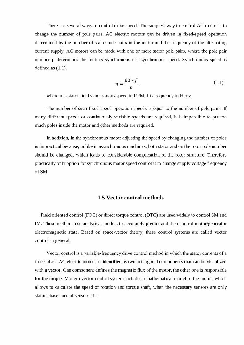
There are several ways to control drive speed. The simplest way to control AC motor is to

change the number of pole pairs. AC electric motors can be driven in fixed-speed operation

determined by the number of stator pole pairs in the motor and the frequency of the alternating

current supply. AC motors can be made with one or more stator pole pairs, where the pole pair

number p determines the motor's synchronous or asynchronous speed. Synchronous speed is

defined as (1.1).

𝑛 =60 ∗ 𝑓

𝑝 ,

where n is stator field synchronous speed in RPM, f is frequency in Hertz.

The number of such fixed-speed-operation speeds is equal to the number of pole pairs. If

many different speeds or continuously variable speeds are required, it is impossible to put too

much poles inside the motor and other methods are required.

In addition, in the synchronous motor adjusting the speed by changing the number of poles

is impractical because, unlike in asynchronous machines, both stator and on the rotor pole number

should be changed, which leads to considerable complication of the rotor structure. Therefore

practically only option for synchronous motor speed control is to change supply voltage frequency

of SM.

1.5 Vector control methods

Field oriented control (FOC) or direct torque control (DTC) are used widely to control SM and

IM. These methods use analytical models to accurately predict and then control motor/generator

electromagnetic state. Based on space-vector theory, these control systems are called vector

control in general.

Vector control is a variable-frequency drive control method in which the stator currents of a

three-phase AC electric motor are identified as two orthogonal components that can be visualized

with a vector. One component defines the magnetic flux of the motor, the other one is responsible

for the torque. Modern vector control system includes a mathematical model of the motor, which

allows to calculate the speed of rotation and torque shaft, when the necessary sensors are only

stator phase current sensors [11].

(1.1)

Vector control systems measures motor currents and calculates voltages and can accurately

estimate machine state and control torque/flux and rotational speed almost independently and in

real time [12].

Different control methods, mentioned above, are shown in fig. 1.7.

Fig. 1.7. Different control methods used for AC drives

According to the cross-field principle, torque and force reaches a maximum, when the

current and flux linkage vectors are perpendicular. In other words, the angle between these vectors

is 90 electrical degrees. These vectors are always perpendicular in fully compensated DC

machines, because of their compensating and commutating-pole windings. However, the angle

between these vectors in AC machines varies depending on the situation and the machine type.

The basic idea behind a vector-based controller is to bring the current and flux linkage space

vectors as close to perpendicular as possible. As a result, the approach is commonly referred to as

vector control. Field-Oriented Control (FOC) realizes the basic vector control principles. The

machine current is divided to two parts, first affect flux and other produces torque and force.

So excitation and torque/force can be separately controlled. The FOC approach requires

coordinate transformation and motor equivalent circuit analysis. The biggest problem with the

FOC control method is its total reliance on machine inductance and resistance parameters, which

Variable frequency drives

Scalar control Vector control

FOC

DTC

can vary significantly as functions of torque/force and air-gap flux. A model of inductance

behavior is required to make FOC work well.

Direct Torque Control (DTC) does not have current control loops, but controls directly the

motor flux and torque using optimal voltage vector selection. It uses the same electrical current

model and the same inductance parameters as FOC for magnetic flux estimation, but additionally

other stabilization techniques for control stabilization. The DTC method can be considered as a

kind of synthesis method that is designed to combine the good properties of different control

methodologies [12]. Both DTC and FOC are suitable control methods for EESM. In this work the

objective is to analyze and implement a FOC version for EESM including also field winding

control loop.

1.6 Converter technology overview

In variable speed AC drives power converter technology has a central role. In its basic

meaning, term “power converter” means the device, which is capable to convert electrical energy

from the grid with given parameters (voltage amplitude, frequency) to the electrical energy with

parameters different from initial ones. For instance, in special case of DC to AC conversion, the

convertor device called invertor.

Vector control requires capability to change both voltage amplitude and frequency, which

is possible with semiconductor-based converters. In the simplest cases, the frequency and voltage

control takes place in accordance with a given characteristic of V/f, in the most advanced

converters use vector control principles described in the previous chapter. From the topological

point-of-view, frequency converters can be classified as shown on fig.1.8.

Fig. 1.8. Classification of frequency converters

The frequency converter consists of the circuits, which include thyristors or transistors,

which operate in the mode of electronic switches. At the heart of the control part is a

microprocessor which provides control signals for power electronic switches, as well as a large

number of decision supporting tasks (monitoring, diagnostics, protection).

Depending on the structure and mode of operation of the electric drive there are two types

of voltage source frequency converters:

With a direct connection.

With the explicit intermediate DC link.

In direct coupled converters power module is presented as a controlled rectifier. The control

system in turn unlock the thyristor groups one by one and connects the motor winding to the supply

grid.

Thus, the output voltage is formed from the "cut" portions of the input voltage sine waves.

Output frequency of such transducers cannot be equal to or higher than the supply frequency. It is

in the range from 0 to 30 Hz, and as a consequence - the small control range of engine speed (no

more than 1: 10). This limitation does not allow to apply such converters in modern variable

frequency drives to control a wide range of process parameters.

The most widely used converter type in modern industry is a converter with intermediate

DC link. This type of converters use a chain of energy conversions: the input sine wave voltage

Frequency converters

Direct converters

Cycloconverters

Matrix converters

DC-link converters

Voltage source

Current source

with constant amplitude and frequency is rectified, passes through the filter, and then converted

back to AC voltage with variable frequency and amplitude.

Electrical circuit of all the control systems based on DC-link topology is shown on fig. 1.9.

Fig. 1.9. Typical AC-AC frequency converter with DC-link inside

Different control algorithms and principles (FOC or DTC) can be applied to the converter

topology shown above.

2. Drive system modelling and mathematical model description

In this chapter it is described the basic ideas of implementation theoretical background into

simulation model of real drive system.

Motor control system development was started by implementing a motor control system

simulink model, which includes 2 major parts – control algorithm blocks and hardware simulation

blocks. Fig. 2.1 shows a general structure of simulation model and fig. 2.2. shows the

corresponding Simulink model.

Fig. 2.1. Designed block-scheme of whole control-motor system [13]

Fig. 2.2. Drive system model built in Simulink

On fig. 2.1 the control logic part, which should be implemented inside of microcontroller, is

highlighted (“Control”-block in fig. 2.2). VSI block is a power electronics based converter, which

provides a supply voltage according to control signals generated by control logic blocks. Also

motor simulation block is included into Simulink model (EESM on the fig. 2.1). For practical

implementation of the control concept, the control logic part is the most important part of the

simulation model, because in these blocks all the needed mathematics and estimations must be

done, and all the operations designed in this blocks set must be transferred to the controller.

Basically, the task of the control logic part is to generate an appropriate switch signals for

the semiconductor bridge in a way to keep motor speed equal to reference speed, given by user.

Therefore, control logic has an input of reference speed, output as a control signals, and a number

of feedback signals from the motor.

Field Oriented control, as far as other types of vector control, is based on the idea to put

current space vector to desired direction with desired length.

The space vector theory itself has the following meaning. It is known, that 3-phase winding

in the machine stator produces a rotating magnetic field. Three phase currents can be represented

by a single space vector showing the combined current effect of 3-phase winding system. (fig. 2.3,

2.4).

Fig. 2.3 Physical implementation of the space vector theory [16].

Fig.2.4. Illustration of three phase currents system to one space vector transformation.

Mathematically, space vector can be calculated using equation:

𝑢𝑠(𝑡) =2

3(𝑎0 𝑢𝑠𝑈(𝑡) + 𝑎1 𝑢𝑠𝑉(𝑡) + 𝑎2 𝑢𝑠𝑊(𝑡))

where 𝑢𝑠 – space voltage vector, a is a phase-shift operator 𝑎 = 𝑒𝑗2𝜋

3 , 𝑢𝑠𝑈, 𝑢𝑠𝑉, 𝑢𝑠𝑊 – stator

cvoltages in phase U, V, W respectively.

(2.1)

In present control system, two axis approach is used. It is based on transforming the three-

phase variables into a rotating vector (space vector), which then can be transformed into two-phase

system.

Initially, a current control unit produces a desired space vector voltage referred in dq-

coordinate system (in rotor reference frame). Voltages in dq-coordinates are transforming into αβ-

coordinates, which are stator based coordinates.

Coordinate transformation between rotor (dq, also called general reference frame) and stator

(αβ) reference frames can be done using equations (2.2).

𝑢𝑠𝛼𝑠 = 𝑢𝑠𝑑

𝑔cos 𝜔𝑔𝑡 − 𝑢𝑠𝑦

𝑔sin 𝜔𝑔𝑡

𝑢𝑠𝛽𝑠 = 𝑢𝑠𝑑

𝑔sin 𝜔𝑔𝑡 + 𝑢𝑠𝑞

𝑔 cos 𝜔𝑔𝑡

where 𝑢𝑠𝑑𝑔

, 𝑢𝑠𝑞𝑔

- d- and q- voltage components of space vector 𝑢𝑠 in general reference frame,

𝜔𝑔 - general reference frame angular speed

After that, αβ-coordinates transforming into 3-phase ABC system using equations (2.3),

reference phase values can be sent to the modulator bridge.

[

𝑢𝑠𝑈

𝑢𝑠𝑉

𝑢𝑠𝑊

] = [cos 𝑘 sin 𝑘 1

cos(𝑘 + 120°) sin(𝑘 + 120°) 1cos(𝑘 + 240°) sin(𝑘 + 240°) 1

] [

𝑢𝑠𝛼𝑠

𝑢𝑠𝛽𝑠

𝑢𝑠0𝑠

]

where 𝑢𝑠𝛼𝑠 , 𝑢𝑠𝛽

𝑠 – α- and β- voltage components of space vector 𝑢𝑠 in stator reference frame,

𝑢𝑠0𝑠 - possible zero sequence voltage component, 𝑘 - phase shift angle between the U-axis and the

x-axis.

When a current feedback goes back to the current control block, ABC- to dq-coordinates

transformation occurs back.

Reasons of doing these transformations is that the controller response speed is not infinite,

so when reference value is changing, controller does not instantly work out. If the reference is

constantly changing, like a sine wave, the controller will try all the time to catch it up, never

reaching. And with an increase of the motor speed, of actual current lag behind from the target

will be more and more. To avoid this, in the model are introduced blocks of coordinate

transformations. They do a very simple thing: firstly, transforms a current space vector created by

(2.3)

(2.2)

three-phase windings into 2-phase representation (basically, by making a space vector projection

to ɑ and β axis) and then turning on an input vector by a predetermined angle. Coordinate

transformation block which transfers the space vector from dq- to ɑβ-coordinates turns the space

vector to the angle + Θ, and back coordinate transformation from ɑβ- to dq-coordinates occurs by

rotating a space vector to the angle -Θ.

Straight coordinate transformation block (ɑβ to dq) makes coordinate transformation for

transferring the currents from fixed axes α and β, attached to the motor stator to the rotating axes

d and q, attached to the motor rotor (using the rotor position angle Θ). A back coordinate

transformation block (dq to ɑβ) makes inverse transform of the reference voltage on axes d and q

axes makes the transition to the α and β axes.

Thanks to such transformations, instead of «rotation» of regulators reference value, we rotate

their inputs and outputs, and the regulators themselves operate in static mode: current d, q, and

controller output are constant in the steady mode, as shown in the fig. 2.5. The axes d and q rotating

together with the rotor (as they are rotated by a signal from the rotor position sensor). Current

regulators do not even know that something somewhere is rotating. They work in static mode:

adjusting each of its current (d and q), reaching the reference voltage - and keep it constant, all the

work of making a turn is the task of blocks of coordinate transformations.

So, using the reference frame transformations in control system gives us a benefits like

fundamental frequency appears as dc quantity, simple linear controllers (e.g. PI) can be applied

and it enables to achieve zero steady-state error.

Fig. 2.5. Stator-based and rotor-based reference frames representation: a) Space vector

decomposition in stationary αβ-frame and synchronous dq-frame for current space vector as an

example; b) Rotating space vector projection to αβ axes [13]; c) Rotating space vector projection

to dq axes [13]

Synchronous machine model is built using equivalent circuits as shown on fig. 2.6.

Fig. 2.6. Synchronous machine equivalent circuits for d ad q-axes [14]

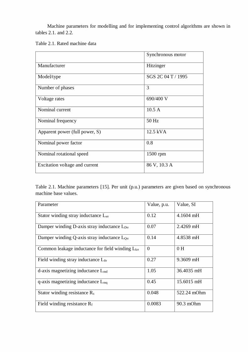
Machine parameters for modelling and for implementing control algorithms are shown in

tables 2.1. and 2.2.

Table 2.1. Rated machine data

Synchronous motor

Manufacturer Hitzinger

Model/type SGS 2C 04 T / 1995

Number of phases 3

Voltage rates 690/400 V

Nominal current 10.5 A

Nominal frequency 50 Hz

Apparent power (full power, S) 12.5 kVA

Nominal power factor 0.8

Nominal rotational speed 1500 rpm

Excitation voltage and current 86 V, 10.3 A

Table 2.1. Machine parameters [15]. Per unit (p.u.) parameters are given based on synchronous

machine base values.

Parameter Value, p.u. Value, SI

Stator winding stray inductance Lsσ 0.12 4.1604 mH

Damper winding D-axis stray inductance LDσ 0.07 2.4269 mH

Damper winding Q-axis stray inductance LQσ 0.14 4.8538 mH

Common leakage inductance for field winding Lkσ 0 0 H

Field winding stray inductance Lfσ 0.27 9.3609 mH

d-axis magnetizing inductance Lmd 1.05 36.4035 mH

q-axis magnetizing inductance Lmq 0.45 15.6015 mH

Stator winding resistance Rs 0.048 522.24 mOhm

Field winding resistance Rf 0.0083 90.3 mOhm

Parameters presented in table 2.1 are measured using methods presented in the standards

IEC 34-4 “Methods for determining synchronous machine quantities from tests” and IEEE

Standard 115-1983 “Test procedures for synchronous machines”. The values measurement process

is described in [12].

For control parameters calculation, further in this chapter, we are also interested in following

machine parameters:

𝐿𝑑 = 𝐿𝑠𝜎 + 𝐿𝑚𝑑 = 0.12 + 1.05 = 1.17 𝑝. 𝑢. = 40.56 𝑚𝐻;

𝐿𝑞 = 𝐿𝑠𝜎 + 𝐿𝑚𝑞 = 0.12 + 0.45 = 0.57 𝑝. 𝑢. = 19.76 𝑚𝐻;

𝐿𝐷 = 𝐿𝐷𝜎 + 𝐿𝑚𝑑 + 𝐿𝑘𝜎 = 0.07 + 1.05 + 0 = 1.12 𝑝. 𝑢. = 38.83 𝑚𝐻;

𝐿𝑄 = 𝐿𝑄𝜎 + 𝐿𝑚𝑞 = 0.14 + 0.45 = 0.59 𝑝. 𝑢. = 20.46 𝑚𝐻;

𝐿𝑓 = 𝐿𝑓𝜎 + 𝐿𝑚𝑑 + 𝐿𝑘𝜎 = 0.27 + 1.05 + 0 = 1.32 𝑝. 𝑢. = 45.76 𝑚𝐻

Synchronous machine model consists of the block modeling the electrical processes taking

place in the machine, as well as the mechanical model of the machine. Electrical model uses as the

input parameters phase voltages and the voltage across the field winding. The primary output of

the machine model is electromagnetic torque is defined by

𝑇𝑒 =3

2𝑝 (𝜓𝑠𝑑 𝑖𝑞 − 𝜓𝑠𝑞 𝑖𝑑)

The model estimates flux linkage 𝜓𝑠𝑑 and 𝜓𝑠𝑞 based on stator voltage, while stator currents

𝑖𝑠𝑞 and 𝑖𝑠𝑑 are based on measured phase currents and coordinates transformation. Stator flux can

be also estimated using measured DC voltage and switching states. In addition, model uses

measured field current as an input. The mechanical model of the machine calculates rotor speed

using electromagnetic torque Te, load torque Tload and motor inertia Jmech

𝑇𝑒 − 𝑇𝑙𝑜𝑎𝑑 = 𝐽𝑚𝑒𝑐ℎ

𝑑

𝑑𝑡 𝜔𝑚𝑒𝑐ℎ

Found values are switched to the control block as a feedback signals.

The main part of machine vector control are control loops for stator current components (id,

iq). The stator current control equations are implemented after reference frame transformation as

PI-controllers for d- and q-axis currents. The outputs of the stator current controller are connected

to the modulator in real application. It is assumed here that modulation process is enabling to

reproduce the output of the controllers perfectly. Additional part of current control are decoupling

algorithms between d- and q-axis.

(2.4)

(2.5)

(2.6)

Also excitation current control, stator flux and speed controls are based on using PI-

controllers, which can be tuned according to Internal Model Control (IMC) Method [17]. Below

general information about the IMC method is given. Later in subchapters 2.1 – 2.4 more

explanation for tuning controller parameters is given.

IMC is a method for tuning PI-controllers parameters, which allows to tune control of d and

q components of the stator current at the same time and without cross-coupling between d and q

components. In other words, two PI controllers, which are responsible for d- and q-axes values,

can be tuned together. This method is applied in synchronous-frame PI controllers. The controller

parameters are expressed directly in machine parameters and the desired closed loop bandwidth.

Fig. 2.7. a) Classical PI control structure b) General picture of IMC structure [17]

On fig. 2.7a a classical PI control system is given, while fig. 2.7 b shows the IMC structure.

The IMC structure uses an internal model �̂�(𝑠) in parallel with the controlled system (plant) 𝐺(𝑠).

For an AC machine, u and y are respectively the stator voltage and current vectors, 𝑟 =

[𝑖𝑑𝑟𝑒𝑓

, 𝑖𝑞𝑟𝑒𝑓]

𝑇 is the current reference vector. The control loop is augmented by a block 𝐶(𝑠) - the

so-called IMC controller. �̂�(𝑠), 𝐺(𝑠), 𝐶(𝑠) are all transfer function matrices [17].

The main benefit of using IMC is that the tuning problem, which for a PI controller involves

adjustment of two parameters for two PI-controllers, is reduced to the selection of one parameter

only, the desired closed-loop bandwidth α.

For a first-order system the desired current rise time 𝑡𝑟 is related to bandwidth α as 𝑡𝑟 =

𝑙𝑛(9)

α . Known value of the rise time and α allows immediately define the desired bandwidth and

find a suitable controller parameters.

On fig. 2.8. it is shown special case of using IMC structure with decoupling terms together

and it shows how decoupling terms can be applied to the model. Such topology allows to decouple

machine dynamics before using IMC method. In this case decoupling can be regarded as inner

feedback loop in the plant Gd(s) [17].

Fig. 2.8. IMC structure topology with decoupling.

In fig. 2.8 W is decoupling matrix and Gd(s) is the plant with applied decoupling terms on it.

2.1. Stator current control

The main purpose of the stator current control system is the formation of the desired current

values of the d- and q-axes, which later, after the coordinate transformation and transfer to the

three-phase voltage system, will represent a task for the semiconductor bridge which is responsible

for supplying the motor with appropriate phase voltages. As noticed, the output values of the stator

current control unit are only voltage references on d-and q-axis.

The principle of forming the output voltage based on the use of PI-regulator, the input of

which is fed the static error value between the reference and actual values for current by d- and q-

axis. Reference values of the 𝑖𝑑 𝑟𝑒𝑓 and 𝑖𝑞 𝑟𝑒𝑓 currents are defined by upper level torque and the

flux controllers

The current controllers are tuned according to IMC method, therefore first it was determined

decoupling terms, which are implemented in the model according equations (2.7), (2.8).

Decoupling terms calculation and EESM tuning example can be found in [13].

𝑒𝑑 = −𝐿𝑚𝑑𝑅𝐷

𝐿𝐷 𝑖𝐷 + 𝐿𝑚𝑑 (1 −

𝐿𝑚𝑑

𝐿𝐷)

𝑑𝑖𝑓

𝑑𝑡− 𝜔𝜓𝑞

𝑒𝑞 = −𝐿𝑚𝑞𝑅𝑄

𝐿𝑄 𝑖𝑄 + 𝜔𝜓𝑑

After collecting the machine parameters (Tables 2.1, 2.2) and choosing desired rise time tr ,

it becomes possible to calculate all the controller’s parameters.

As a first estimation for choosing desired current rise time, we can remember that motor

torque respond speed id directly connected with q-axis current rise time. Let’s assume

(2.8)

(2.9)

(2.7)

that desired torque respond time must be 5 ms, because this value gives us an appropriate speed of

machine respond suitable for major industrial applications. We can conclude that initial value of

current rise time must be selected 𝑡𝑟 = 5 ms. After determined rise time, we can find bandwidth α

(for using DIMC method):

𝛼 =ln 9

𝑡𝑟=

ln 9

0.005= 439.44 𝐻𝑧

Then we can find PI coefficients for d and q axis controllers using equations (2.10) – (2.14),

given in [17]. Here we should mention that coefficients calculations must be done in SI units.

𝐿𝑐𝑐𝑑 = 𝐿𝑑 −𝐿𝑚𝑑

2

𝐿𝐷= 0.0405639 −

0.03640352

0.0388304= 6.4356 𝑚𝐻

𝐾𝑝𝑑 = 𝛼 ∗ 𝐿𝑐𝑐𝑑 = 2.85

𝐿𝑐𝑐𝑞 = 𝐿𝑞 −𝐿𝑚𝑞

2

𝐿𝑄= 0.0197619 −

0.01560152

0.0204553= 7.8624 𝑚𝐻

𝐾𝑝𝑞 = 𝛼 ∗ 𝐿𝑐𝑐𝑞 = 3.46

𝐾𝑖𝑑 = 𝐾𝑖𝑞 = 𝛼 ∗ 𝑅𝑠 = 439.44 ∗ 0.52224 = 230

Coefficients, received in (2.11), (2.14) and (2.14) by DIMC method can be directly used in

model’s PI controller determining.

2.2. Excitation Current Control

The excitation current control is carried out by setting a corresponding voltage to the

excitation winding, which is calculated on the basis of the required excitation current, the actual

excitation current and 𝑖𝐷 and 𝑖𝑠𝑑 currents. The desired excitation current value is based on the

principle of unity power factor control and reference values 𝑇𝑟𝑒𝑓 and 𝜓𝑠 𝑟𝑒𝑓 .

Processing the desired value and the actual value of the excitation current is performed on

the basis of PI-regulator (fig. 2.9).

(2.10)

(2.11)

(2.12)

(2.13)

(2.14)

Fig. 2.9. Excitation current PI controller structure

As in stator current control, here IMC method is used. According to this method, decoupling

term (2.15) was implemented in the model [17]:

𝑒𝑓 = −𝐿𝑚𝑑𝑅𝐷

𝐿𝐷𝑖𝐷 + 𝐿𝑚𝑑 (1 −

𝐿𝑚𝑑

𝐿𝐷)

𝑑𝑖𝑑

𝑑𝑡

PI controller parameters can found using equations (2.17), (2.18). The rise time for excitation

current must be bigger than stator current rise time because the rotor time constant is usually larger

than the stator time constant. This is the reason why for fast torque changes it is reasonable to use

stator current tuning mostly. While machine operates we are trying to keep flux linkage constant

and change it only is field weakening is needed. In accordance to all mentioned above we can

assume 𝑡𝑟𝑓 = 5.5 𝑚𝑠. The 𝛼 coefficient in this case will be (2.16):

𝛼𝑓 =ln 9

𝑡𝑟= 399 Hz

After collecting machine parameters 𝑅𝑓 , 𝐿𝑓, 𝐿𝑓𝐷 , 𝐿𝐷 from table 2.1 and equations (2.4) we

can calculate:

𝐾𝑝𝑓 = 𝛼𝑓 (𝐿𝑓 −𝐿𝑓𝐷

2

𝐿𝐷) = 399.5 (45.644 −

36.40352

38.8304) ∗ 10−3 = 4.69

𝐾𝑖𝑓 = 𝛼𝑓 𝑅𝑓 = 399.5 ∗ 0.0903 = 36

Integrator time can be now found as:

𝑇𝑖𝑓 =𝐾𝑝𝑓

𝐾𝑖𝑓= 0.13 𝑠

Calculated values in (2.17), (2.19) can be applied in field current PI-controller.

(2.15)

(2.16)

(2.18)

(2.19)

(2.20)

2.3. Speed Control

Adjusting the motor speed is accomplished by controlling the required torque. Thus, to

control the motor rotational speed, the speed control unit produces on the output the desired torque

required to achieve a reference speed value. After that, the vector control system tries to provide a

given torque on the motor shaft. Speed control is based on the use of PI-regulator.

Fig. 2.10 Speed controller structure [13]

On fig. 2.10 current controller is shown as GCC (s), and speed controller is GPI (s). Tuning of

the speed controller parameters is done by the following way.

As far as speed controller becomes an outer control loop for q-axis current control,

mentioned in chapter 2.1, integrator time can be found based on time for current control and

symmetric optimum rule (if we have outer loop, it must be slower than inner control loop) we can

take 𝑇𝑖𝜔 = 4 ∗ 𝑇𝑖𝑐𝑐 = 0.04924 s, and α value is calculated in similar way to current control.

Gain values for speed and flux controllers can be found using root locus analysis and further

load sensitivity function analysis. Root locus analysis is used as a first estimation approach. For

final gain coefficients determination load sensitivity function analysis is applied.

Open loop transfer function for speed controller is:

𝐺𝑇,𝑜𝑙 =𝐾𝑝𝜔(𝑇𝑖𝜔 𝑠 + 1)

𝑇𝑖𝜔𝑠

𝛼𝐶𝐶

𝑠 + 𝛼𝐶𝐶 1

𝐽𝑠=

22.68 𝑠 + 439.4

0.00516 𝑠3 + 2.268 𝑠2

where 𝐾𝑝𝜔 was taken as 1, 𝑇𝑖𝜔 = 4 ∗ 𝑇𝑖𝑐𝑐 and 𝛼𝐶𝐶 is a bandwidth found in stator current control

calculation, 𝐽 = 0.1 kgm2 is the machine moment of inertia.

According to open loop transfer function (2.21), root locus was built (fig. 2.11) using Matlab

environment. The Matlab script which implements all the graphical representations above (fig.

2.11 – 2.15) presented in appendix 1.

(2.21)

Fig. 2.11. Root locus for speed-responsible open-loop transfer function

From fig. 2.11 we can see, that the most suitable gain should be located at real axis (to avoid

oscillations in the system) or have damping factor not smaller than 0.9. From this point of view,

gain Kpw=5 is selected. The maximum value for required damping = 0.9 is Kpw = 14.4.

In addition to root locus we also must analyze control system from the disturbance rejection

point of view.

The open loop transfer function mentioned earlier (2.21) becomes a multiplication P(s) C(s),

where 𝐶(𝑠) =𝐾𝑝𝜔(𝑇𝑖𝜔 𝑠+1)

𝑇𝑖𝜔𝑠

𝛼𝐶𝐶

𝑠+ 𝛼𝐶𝐶 is a multiplication stator current control, which is inner loop

control, and the speed control, which is outer loop control. Plant in the speed control loop becomes

𝑃(𝑠) =1

𝐽𝑠 .

To analyze load response performance we are interested in load sensitivity function analysis,

which is transfer function from input disturbance Di(s) to output Y(s):

𝐺𝑑𝑦(𝑠) =𝑌(𝑠)

𝐷𝑖(𝑠)=

𝑃(𝑠)

1+𝑃(𝑠)𝐶 (𝑠)

On fig. 2.12 – 2.14 it is shown analysys of the load sensitivity function (2.22) with applying

different gains. Fig. 2.12 presents a Nyquist diagram for open-loop sensitivity

function 𝑃(𝑠) ∗ 𝐶(𝑠).

Fig. 2.12. Nyquist Diagram for Sensitivity function analysis for speed controller

(2.22)

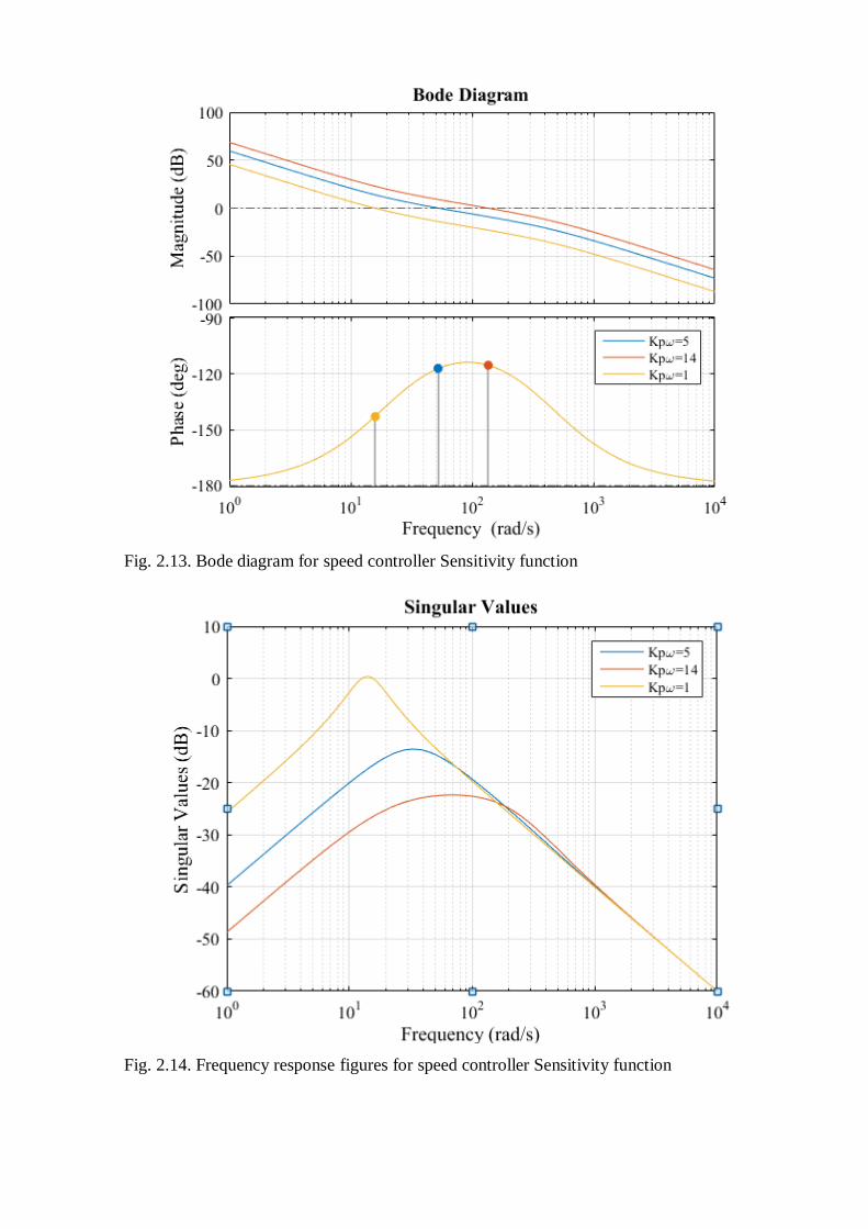
Fig. 2.13. Bode diagram for speed controller Sensitivity function

Fig. 2.14. Frequency response figures for speed controller Sensitivity function

2.15. Step response of the system for input disturbance

According to Nyquist plot (fig. 2.12), and Bode diagram (fig. 2.13) controller with parameter

𝐾𝑝𝑤 = 5 and 14 provides more robust control than with parameter 𝐾𝑝𝑤 = 1. From fig. 2.13 we

can see that gain values 𝐾𝑝𝑤 = 5 and 14 provides almost equal stability phase margin. From the

frequency response figure (fig. 2.14) we can notice that increasing the gain makes system better

from the disturbance rejection point of view. On fig. 2.14 we can see that controller with

parameters 𝐾𝑝𝑤 = 5 and 14 damps the disturbance effective across whole frequency band.

Fig. 2.15 shows that controller with 𝐾𝑝𝑤 = 14 provides the lowest peak response for external

disturbance injection as far as peak observed with 𝐾𝑝𝑤 = 5 becomes about two times higher

transient process time remains same as for 𝐾𝑝𝑤 = 14.

Here and further in flux control tuning it is also important to remember that it is not

reasonable to ask too high gain values. When gain becomes higher, it makes higher peak voltage

references in transient mode and overcurrent may occur during the drive system operation. It is

important to tune gains in accordance with physical limitations of used hardware and avoid gain

values which can cause overvoltage in the system. Taking into account that gains 𝐾𝑝𝑤 = 5 and 14

has almost same phase stability margins and both provides satisfactory frequency and step

responses, it is more preferable to take lower possible gain.

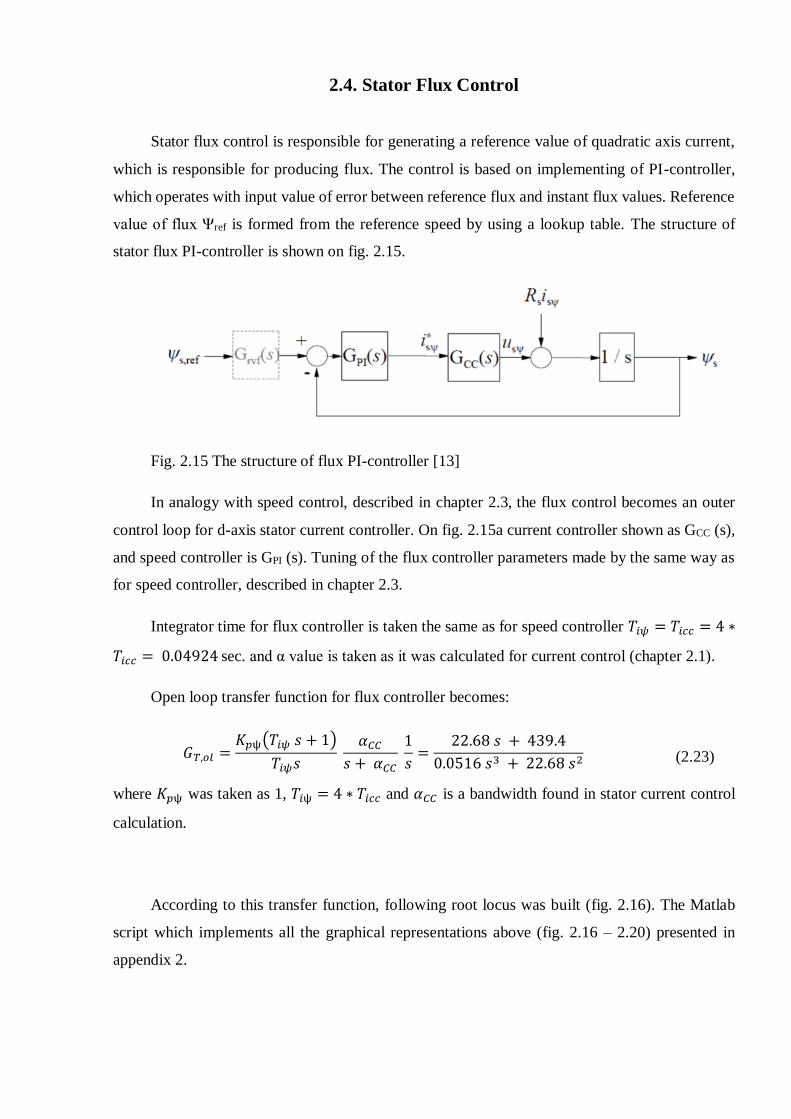
2.4. Stator Flux Control

Stator flux control is responsible for generating a reference value of quadratic axis current,

which is responsible for producing flux. The control is based on implementing of PI-controller,

which operates with input value of error between reference flux and instant flux values. Reference

value of flux Ψref is formed from the reference speed by using a lookup table. The structure of

stator flux PI-controller is shown on fig. 2.15.

Fig. 2.15 The structure of flux PI-controller [13]

In analogy with speed control, described in chapter 2.3, the flux control becomes an outer

control loop for d-axis stator current controller. On fig. 2.15a current controller shown as GCC (s),

and speed controller is GPI (s). Tuning of the flux controller parameters made by the same way as

for speed controller, described in chapter 2.3.

Integrator time for flux controller is taken the same as for speed controller 𝑇𝑖𝜓 = 𝑇𝑖𝑐𝑐 = 4 ∗

𝑇𝑖𝑐𝑐 = 0.04924 sec. and α value is taken as it was calculated for current control (chapter 2.1).

Open loop transfer function for flux controller becomes:

𝐺𝑇,𝑜𝑙 =𝐾𝑝ψ(𝑇𝑖𝜓 𝑠 + 1)

𝑇𝑖𝜓𝑠

𝛼𝐶𝐶

𝑠 + 𝛼𝐶𝐶 1

𝑠=

22.68 𝑠 + 439.4

0.0516 𝑠3 + 22.68 𝑠2

where 𝐾𝑝ψ was taken as 1, 𝑇𝑖ψ = 4 ∗ 𝑇𝑖𝑐𝑐 and 𝛼𝐶𝐶 is a bandwidth found in stator current control

calculation.

According to this transfer function, following root locus was built (fig. 2.16). The Matlab

script which implements all the graphical representations above (fig. 2.16 – 2.20) presented in

appendix 2.

(2.23)

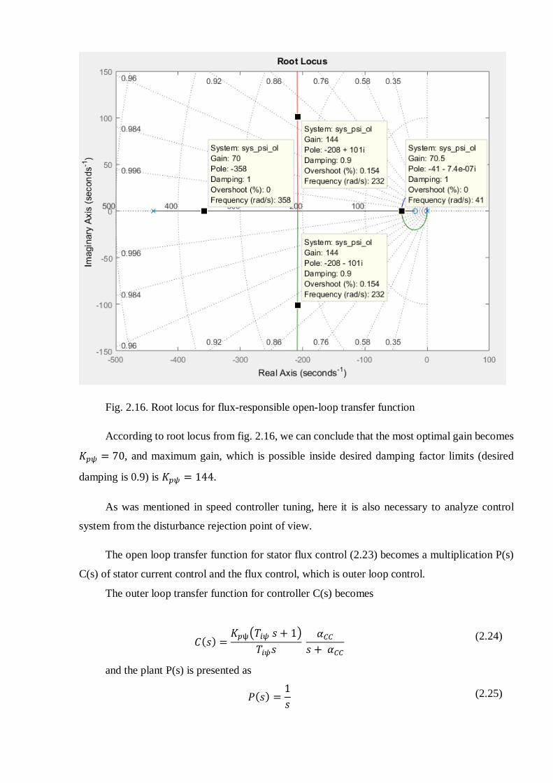
Fig. 2.16. Root locus for flux-responsible open-loop transfer function

According to root locus from fig. 2.16, we can conclude that the most optimal gain becomes

𝐾𝑝𝜓 = 70, and maximum gain, which is possible inside desired damping factor limits (desired

damping is 0.9) is 𝐾𝑝𝜓 = 144.

As was mentioned in speed controller tuning, here it is also necessary to analyze control

system from the disturbance rejection point of view.

The open loop transfer function for stator flux control (2.23) becomes a multiplication P(s)

C(s) of stator current control and the flux control, which is outer loop control.

The outer loop transfer function for controller C(s) becomes

𝐶(𝑠) =𝐾𝑝ψ(𝑇𝑖𝜓 𝑠 + 1)

𝑇𝑖𝜓𝑠

𝛼𝐶𝐶

𝑠 + 𝛼𝐶𝐶

and the plant P(s) is presented as

𝑃(𝑠) =1

𝑠

(2.24)

(2.25)

To analyze load response performance we are interested in load sensitivity function (2.26)

analysis.

𝐺𝑑𝑦(𝑠) =𝑌(𝑠)

𝐷𝑖(𝑠)=

𝑃(𝑠)

1+𝑃(𝑠)𝐶 (𝑠)

On fig. 2.19 – 2.20 show analysis of the load sensitivity function (2.26) with applying

different gains. Nyauist (fig. 2.17) and Bode (fig2.18) diagrams was built for open-loop system

𝑃(𝑠) ∗ 𝐶(𝑠)

Fig. 2.17. Nyquist Diagram for flux controller Sensitivity function

(2.26)

Fig. 2.18. Bode diagram for flux controller Sensitivity function

Fig. 2.19. Frequency response figures for flux controller Sensitivity function

2.20. Step response of the system for input disturbance

From the figures 2.19 we can find, that initially found gain provides appropriate disturbance

rejection level, so it is not necessary to increase stability margin much, and increasing the gain

coefficient by almost 4 gives us small increasing in disturbance rejection (fig. 2.20). The value

𝐾𝑝𝛹 = 300 has better stability than 𝐾𝑝𝛹 = 70 and applied in the model. From fig. 2.19 we can

find that all the gains allow the system effectively to damp the disturbance across the whole

frequency band. Analyzing Nyquist plot (fig. 2.12) we can conclude that increasing the gain

decreases a little system stability, but system becomes better from disturbance rejection point of

view.

2.5. Model running

Model initially was developed for variable-step ode23tb solver. The principal structure of

the Simulink model presented in fig. 2.21.

Fig. 2.21 a. General view of the model topology in Simulink environment

Fig. 2.21 b. Blocks under the EESM drive mask represents general parts of the drive system.

Running scenario for testing and investigating the model is 10 seconds run with reference

speed of 1500 rpm and giving a load of 92.3 Nm after 8 second from start. To check the motor

status it was decided to monitor the actual speed of the shaft and stator voltages 𝑈𝑠𝑑 and 𝑈𝑠𝑞 . After

test simulations with different parameters obtained results are shown on fig. 2.21 a - d.

2.21 a. Simulation results for 𝐾𝑝𝜔 = 1 and 𝐾𝑝𝜓 = 140

2.21 b. Simulation results for 𝐾𝑝𝜔 = 1 and 𝐾𝑝𝜓 = 300

2.21 c. Simulation results for 𝐾𝑝𝜔 = 5 and 𝐾𝑝𝜓 = 140

2.21 d. Simulation results for 𝐾𝑝𝜔 = 5 and 𝐾𝑝𝜓 = 300

The implementation of desired behavior and creation of the code for controller programming

is described in chapter 4, after review of hardware equipment.

3. Hardware description

In this chapter hardware based part of the project is discussed. A description of existing

equipment given. Also implementation of the analyzed control system using existing equipment is

discussed.

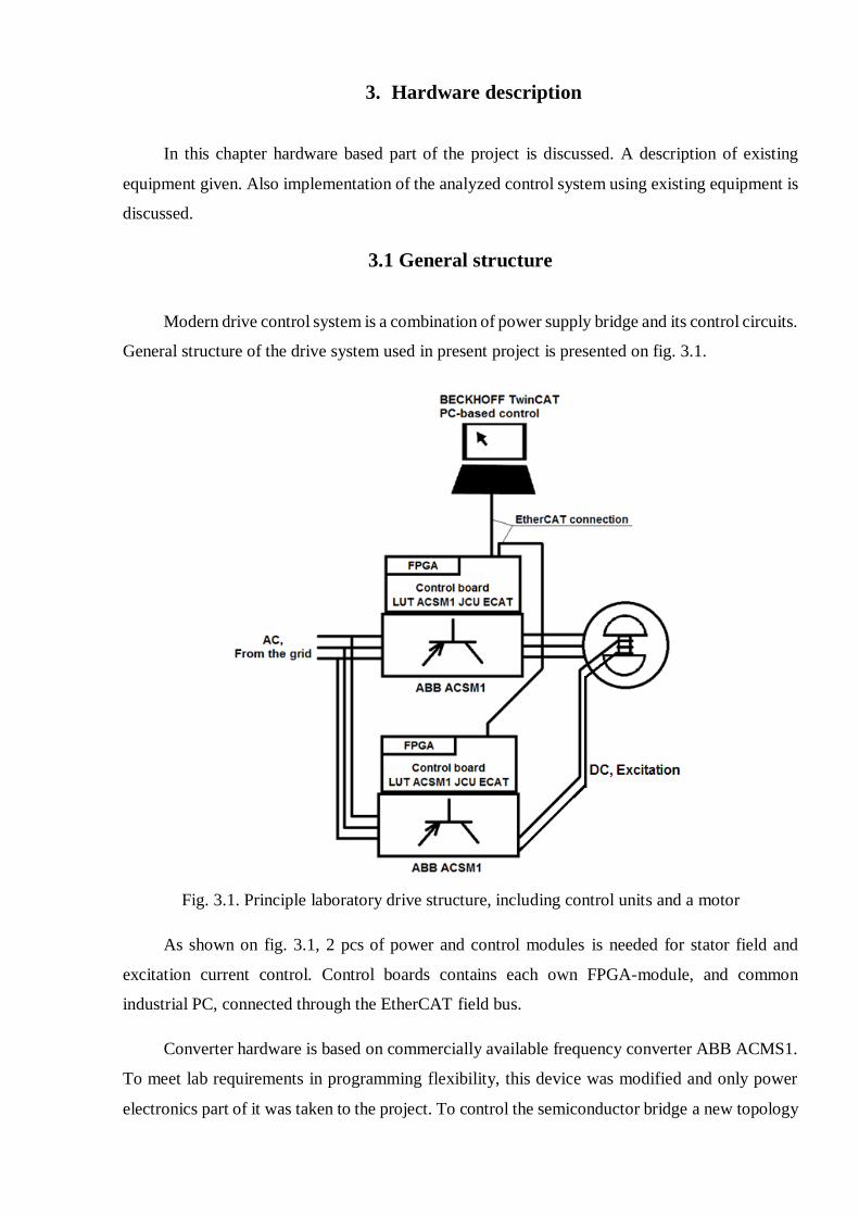
3.1 General structure

Modern drive control system is a combination of power supply bridge and its control circuits.

General structure of the drive system used in present project is presented on fig. 3.1.

Fig. 3.1. Principle laboratory drive structure, including control units and a motor

As shown on fig. 3.1, 2 pcs of power and control modules is needed for stator field and

excitation current control. Control boards contains each own FPGA-module, and common

industrial PC, connected through the EtherCAT field bus.

Converter hardware is based on commercially available frequency converter ABB ACMS1.

To meet lab requirements in programming flexibility, this device was modified and only power

electronics part of it was taken to the project. To control the semiconductor bridge a new topology

was designed instead of standard control board. The new control layout LUT ACSM1 JCU ECAT

circuit board operates using a FPGA (Field-Programmable Gate Array) – matrix, and a computer

with specific running software on it. Also industrial computer can be used instead of desktop PC.

Control tasks, described in chapter 2, were divided between FPGA and computer hardware units

in order to make the easiest and fast control system. Fig. 3.2 shows, which tasks are implemented

in each of them.

Fig. 3.2 Using FPGA and PC-based control together [13]

Using described control system hardware, it becomes possible to operate power electronics

switches freely in different modes and change number of parameters, which is necessary for future

lab research projects. At the output of the converter, voltage for motor and its excitation winding

feeding is formed according to desired control algorithms.

3.2. Electromechanical part

In a drive system, which is the object of investigation in current project, a 12.5 kVA

electrically excited synchronous motor is used. For simulating a load torque, induction motor is

connected on the one shaft (fig. 3.3). It runs in the brake mode (slip > 1) when load simulation is

needed. If load torque simulation is not needed, induction motor becomes switched off and rotates

freely by synchronous machine. Induction machine is controlled by its own PWM control system

and this system is not considered in current thesis. Synchronous machine parameters was given in

table 2.1, and induction machine parameters are given in table 3.1.

Fig. 3.3. Synchronous motor (at the left), which is driven by vector control considered in the

current project and induction machine (at the right) for simulating load torque

Table 3.1. Induction machine parameters

Induction machine parameters

Manufacturer Oy Strömberg Ab

Model/type HXUR 368G2 B3

Number of phases 3

Voltage rates 380 V star connected

Nominal current 43

Nominal frequency 50

Apparent power (full power, S) 22 kW

Nominal power factor 0.86

Nominal rotational speed 1460 rpm

Test system is equipped with pulse encoder, which generates rotor angle feedback for

vector control.

3.3. Power converter and its control board

Power semiconductor circuit in this project is made on the basis of commercially produced

frequency converter ABB ACMS1 (fig.3.4) [18].

Fig. 3.4. ABB ACSM1 in original equipment

To achieve the desired flexibility capabilities in setup and software changes, some

modifications has been subjected the frequency converter

Standard semiconductor switches control unit was replaced by a more functional one in

terms of programming. The new control topology consists of FPGA control board in conjunction

with the computer control carried out by means Beckhoff TwinCAT3 software. This configuration

allows to use the algorithm developed in Simulink environment and to implement and change the

model described in Chapter 2 by changing the freely programmable control electronics.

Modified control board was developed in the Electrical Engineering laboratory of

Lappeenranta University of Technology and called LUT ACSM1 JCU ECAT (fig. 3.5).

Fig. 3.5 LUT ACSM1 JCU ECAT control board general view [19]

The control board has FPGA DIMM-module Socket and EtherCAT fieldbus connection to

the PCB itself making a single ACSM1 inverter an individual reprogrammable unit, which made

it possible to implement custom control algorithms working on the ACSM1 industrial inverter

[19].

In electrical drive system implemented in the laboratory (as shown on fig. 3.1) two separately

installed ABB ACSM1 units are used, one is responsible for supplying motor stator windings (unit

called «M1») and other is for feeding excitation winding located at the motor’s rotor (unit called

«M2»). Figure 3.6. shows ABB ACSM1 units M1 and M2 connected to the controlled motor.

Fig. 3.6. ABB ACSM1 units connected to the controlled motor

3.4. FPGA

FPGA is a Field-Programmable Gate Array, a semiconductor device that is based on a matrix

of configurable logic blocks (CLBs) connected via programmable interconnects which may be

configured by the user or developer after manufacture. FPGAs are programmed by changing the

operational logic of the principal circuit, for example using the code at the programming language,

which can describe the desired logic. FPGAs may be modified any time in the process of their use.

They consist of configurable logic blocks, such switches with multi-input and single-output (logic

gates). In digital circuits, such switches implement basic binary operations AND, NAND, OR,

NOR, and XOR. In most modern microprocessors logical function blocks are fixed and cannot be

modified. The principal difference is that in FPGA that blocks, its function and configuration of

connections between them may vary with special signals sent to the circuit.

In current project Xilinx Artix-7 FPGA-based Enclustra Mars AX3 DIMM-module is used

(fig. 3.5, 3.6) [20].

Fig. 3.5. Xilinx Artix-7 FPGA-based unit general view [20]

Fig. 3.6. Xilinx Artix-7 FPGA-based Module Architecture [20]

3.5. PC-based Bechoff TwinCAT

PC-controlled part of the system can be driven by a desktop computer or a special industrial

controller. In this project Bechoff TwinCAT 3 control environment based on desktop PC is used.

The software package Beckhoff TwinCAT allows to control industrial devices directly from

the computer using the Ethernet cable. Beckhoff TwinCAT system integrates in Microsoft Visual

studio and provides wide options for testing, control and measurements operations directly from

desktop PC. In current project the TwinCAT XAE package was used. In fig. 3.7. it is shown the

scheme of control algorithm processing, from its developing in Simulink to the implementation on

real drive.

Fig. 3.7. A procedure for the control development

In chapter «Programming» will be described process of transferring the model created in

Simulink to real hardware devices. Also final parameters’ tuning is done at this stage.

Simulink model

C-code generated by

Simulink

Beckhoff TwinCAT XAE

based on Microsoft

Visual Studio reads C-code

A frequency converter

ACSM1 connects to

the PC

Motor can be controlled

from the PC by control

the ACSM1's using

TwinCAT XAE

4. Code processing and laboratory tests preparation

4.1 General information

Simulink model, which presented in Chapter 2, represents the operation of whole electrical

drive system.

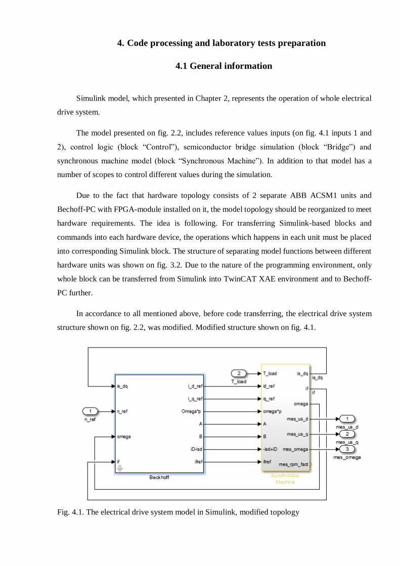
The model presented on fig. 2.2, includes reference values inputs (on fig. 4.1 inputs 1 and

2), control logic (block “Control”), semiconductor bridge simulation (block “Bridge”) and

synchronous machine model (block “Synchronous Machine”). In addition to that model has a

number of scopes to control different values during the simulation.

Due to the fact that hardware topology consists of 2 separate ABB ACSM1 units and

Bechoff-PC with FPGA-module installed on it, the model topology should be reorganized to meet

hardware requirements. The idea is following. For transferring Simulink-based blocks and

commands into each hardware device, the operations which happens in each unit must be placed

into corresponding Simulink block. The structure of separating model functions between different

hardware units was shown on fig. 3.2. Due to the nature of the programming environment, only

whole block can be transferred from Simulink into TwinCAT XAE environment and to Bechoff-

PC further.

In accordance to all mentioned above, before code transferring, the electrical drive system

structure shown on fig. 2.2, was modified. Modified structure shown on fig. 4.1.

Fig. 4.1. The electrical drive system model in Simulink, modified topology

This thesis is mostly focused in Beckhoff PC programming because FPGA needs another

coding environment and skills. Due to that, the main feature of Simulink model structure

modifying is to separate all the tasks and equations designed for implementing by Bechoff-PC,

into separate block. On fig. 4.1 for this purpose it is created a block called “Beckhoff”. As far as

FPGA-matrixes programming is not a focus of current thesis, for simplification all the operations

implemented in FPGAs was moved under the “Synchronous Machine” mask.

For further control and parameters measure, output ports “mes_us_d”, “mes_us_q”,

“mes_omega” was added to measure direct axis stator voltage, quadratic axis stator voltage and

rotational angular speed respectively.

4.2 Simulink to TwinCAT XAE transferring

The interim target of the whole drive system commissioning is to make real drive system

operate in a way as was tested in Simulink. As far as control tasks becomes divided between PC

and FPGA – controlled parts, this parts should be programmed separately.

From programming point of view, the current thesis considers only Beckhoff-PC

programming part. For programming a Beckhoff-PC it used a TwinCAT XAE environment which

is Microsoft Visual Studio integrated system, and also makes connection to Matlab/Simulink

available. For current project purpose, we are interested in possibility to transfer model, developed

in Simulink, into TwinCAT XAE environment.

Code compilation from Matlab Simulink to Beckhoff can be implemented with “Build”

command, which allows to generate a C-code for Bechoff PC directly from the Simulink model.

For code debugging and testing Microsoft Visual Studio with TwinCAT XAE integrated products

is used.

Programming process is shown on fig.4.2.

Fig.4.2. The structure of the whole programming process. Color shows the environment

needed in each step: grey – no environment, blue – working in Matlab Simulink, orange – working

in Microsoft Visual Studio based TwinCAT XAE environment

To make a code for Bechoff PC part (according fig. 3.2), Simulink model was reorganized

to form a separate block which includes exact operations for implementing inside the Beckhoff PC

(Fig. 4.1). After that the model solver options was transferred from variable-step method to discrete

fixed-stepped one. Time step 100 us was selected, since this is the control board sampling

frequency (see fig. 3.6).

Running the drive system

Changing the simulated machine by real machine

Checking the code executing, debugging and correcting model parametres

Loading the C-code project into Microsoft Visual Studio with TwinCAT XAE products

Building the C-code using Simulink “Target For Matlab Simulink” – function

Deviding the model into blocks according to physical topology of control system

Transferring the Simulink model into fixed-step solves, step size is determined by controller requirements

Creation of Simulink model for all the drive chain

Investigation of physical parametres of the synhcronous motor

4.3 Adjusting the model to real hardware requirements

The earlier Simulink simulations were repeated in the TwinCAT XAE environment for

testing the correctness of the compiled code. The simulation results are shown on fig. 4.4. are

slightly different compared to earlier Simulink simulations. (fig. 2.17).

The reason for different results was investigated, and it was found, that a delay of 1 sampling

period appears in TwinCat system, when signal goes from one block to another.

Considering this fact, the Simulink model was modified as shown on fig. 4.3, where delays

of 100 us (1 cycle period) was added between upper-level blocks. After such modification,

Simulink model became operating in a same way as the model transferred in TwinCAT XAE,

developed for Beckhoff PC programming. In this way it was verified, that modified model

corresponded to real system well and TwinCAT XAE simulated results are corresponds results

from Simulink.

Fig. 4.3. Simulink model layout ready for generation of the C-code for Beckhoff PC.

Due to several technical reasons, real laboratory machine becomes possible to operate safety

only with half of it nominal rotational speed. Also due machine safety reasons maximum load

torque given to the machine was limited by 0.9 p.u.

Before laboratory test model is ready, PI-controller coefficients was corrected. Flux

proportional gain reduced from 300 to 0.8. To get better speed behavior speed controller gain was

increased. In laboratory was tested machine behavior with gains corrected to 𝐾𝑝𝜔 = 6.2 and

𝐾𝑝𝜔 = 25. More increasing the speed gain becomes harmful for the motor due to stator

overcurrent appears.

From the investigation described above we can conclude that renewed model topology (fig.

4.3) represents well physical state of the hardware. Optimal found parameters 𝐾𝑝𝜔 = 6.2 − 25

and 𝐾𝑝𝜓 = 0.8 gives reasonable rotor speed behavior and appropriate values of stator voltages.

For further analysis and making conclusions about the simulation model, it becomes obvious to

simulate the model using exactly same scenario as we are going to use while testing in the

laboratory.

4.4 First test simulation

First test simulation happens with 𝐾𝜔 = 6.2 and 𝐾𝜓 = 0.8. Speed increases from 0 to 750

rpm (12.5 Hz, 0.5 p.u.), machine starts after 0.3 seconds after start of observation. After getting

into steady state a load of 0.9 from nominal torque is given. After, load torque goes back to 0.

Results of described simulation scenario are shown on fig. 4.4 – 4.6

Fig. 4.4. Rotor speed reference value and machine model’s shaft behavior for simulation with

𝐾𝜔 = 6.2 and 𝐾𝜓 = 0.8

Fig. 4.5. Stator, damper and field currents behavior simulation using PI-coefficients 𝐾𝜔 = 6.2

and 𝐾𝜓 = 0.8

Fig. 4.6. Reference torque curve for simulation the machine with 𝐾𝜔 = 6.2 and 𝐾𝜓 = 0.8

4.5 Second test simulation

Second test simulation happens with 𝐾𝜔 = 25 and 𝐾𝜓 = 0.8. Speed increases from 0 to

750 rpm (12.5 Hz, 0.5 p.u.), after getting into steady state a load of 0.9 from nominal torque is

given. After, load torque goes to 0. Results of described simulation scenario is shown on fig. 4.7

– 4.10

Fig. 4.7. Rotor speed reference value and machine model’s shaft behavior for simulation with

𝐾𝜔 = 25 and 𝐾𝜓 = 0.8

Fig. 4.7. Stator, damper and field currents behavior simulation using 𝐾𝜔 = 25 and 𝐾𝜓 = 0.8

Fig. 4.8. Reference torque curve for simulation the machine with PI-controllers coefficients 𝐾𝜔 =

25 and 𝐾𝜓 = 0.8

4.3 Code downloading into hardware

The convertors and a machine control can be easily implemented directly from laboratory PC.

Hardware input/output ports are available to control using the same TwinCAT XAE

environment, which was used for advanced model testing. To run a real machine instead of

simulating the process, it is needed to replace signal connections, which goes from Beckhoff

control block to Synchronous motor model (fig. 4.3) by connections to real ports. Control part in

this case remains the same.

Also some additional model tuning was made to meet the requirements of interfacing between

PC and ACSM1 unit.

5. Laboratory tests

In this part will be considered how presented control model works with real machine.

A 12.5 KVA synchronous machine will be run and controlled via TwinCAT XAE environment

using same control logic as used for simulating the drive system. Operation running scenario for

real machine running remains same as used for drive system simulation: free from load

increasing the speed, from 0 to half-nominal speed of 750 rpm, after that putting a step load to

the shaft with a 90% of nominal torque and releasing the machine back to 0 load torque.

Scenario was tested using different PI-gains, respective with first (chapter 4.4) and second

(chapter 4.5) test simulations. Test results was received using TwinCAT XAE environment and

exported into Matlab for curves building.

5.1 First test run

First test represents results of running the system using coefficients 𝐾𝜔 = 6.2 and 𝐾𝜓 = 0.8.

Real machine parameters behavior was recorded and shown on fig. 5.1 – 5.3.

Fig. 5.1. Rotor speed reference value and real machine’s shaft behavior for testing using 𝐾_𝜔 =

6.2 and 𝐾_𝜓 = 0.8

Fig. 5.2. Stator, damper and field currents behavior during the lab test with PI-coefficients

𝐾𝜔 = 6.2 and 𝐾𝜓 = 0.8

Fig. 5.3. Reference torque curve for running machine with PI-controllers coefficients 𝐾𝜔 = 6.2

and 𝐾𝜓 = 0.8

5.2 Second test run

Second test represents results of running the system using coefficients 𝐾𝜔 = 25 and 𝐾𝜓 = 0.8

Fig. 5.4. Rotor speed reference value and real machine’s shaft behavior for testing using

𝐾_𝜔 = 25 and 𝐾_𝜓 = 0.8

Fig. 5.5. Stator, damper and field currents behavior during the lab test with PI-coefficients

𝐾𝜔 = 25 and 𝐾𝜓 = 0.8

Fig. 5.6. Reference torque curve for simulation the machine with PI-controllers coefficients

𝐾𝑝𝜔 = 25 and 𝐾𝑝𝜓 = 0.8

6. Test results processing

As the result of laboratory tests we can present figures 5.1 – 5.6, which shows behavior of a

real machine with different PI-controller parameters. After having this data, it becomes possible

to compare laboratory and simulation results and make a judgment about accuracy of the machine

model was done and about drive simulation process.

In chapter 2.5 it was shown the process of the simulation model development and model

running (fig. 2.21 a-d). After tuning the model, developing the laboratory test scenario and

investigating the most suitable controller gains, a final simulation was done in chapter 4.4 – 4.5.

In mentioned chapters developed drive model was investigated with taking into account laboratory

equipment possibilities and safety issues. It was introduced testing scenario which later was

implemented in the laboratory. The purpose of test results processing becomes to compare values

obtained from model simulation and real machine running, when initial conditions and testing

scenario remains the same. While simulation and later tests it was investigated 2 cases with tuning

different PI-controller parameters.

First, let’s have a look and compare results for investigation the system with PI-controller

parameters 𝐾𝑝𝜔 = 6.3 and 𝐾𝑝𝜓 = 0.8. Simulation of current first case was done in chapter 4.4

and implementation results are given in chapter 5.1.

Fig. 4.4 and 5.1 shows rotor speed behavior for simulation and machine running respectively.

Comparing these data we can notice that real machine operates nicely in the steady state. Speed

curve behavior while lab tests was more smoothly than it was found during the simulation – during

all the lab tests it was no visible speed oscillations at all. Nevertheless, the machine dynamics

becomes slower than it was obtained from simulation. On fig. 5.1 it occurs an overshoot while

reference speed stops to grow up. Speed drop at the load step moment and overshoot when the

load torque was released became larger than while simulation: real speed drop becomes 12% as

far as simulated drop was 10%; the load release overshoot becomes same number difference –

12% for lab tests vs. 10% for simulation.

Comparing machine currents behavior for simulated model (fig. 4.5) and real machine run

(fig. 5.2), we can find that stator, damper and field currents in the steady state observed at identical

values. Analyzing transient modes, we can see that real machine has smoother curves of all the

currents: it becomes no overcurrent peaks at all for stator d- and q- axes currents and field current,

damper current peaks becomes about 50% less that it was obtained from the simulation.

The reference torque behavior simulation result presented on fig. 4.6 and real machine run

result is given on fig. 5.3. In steady state operating the real machine produces small torque (about

0.05 – 0.1 p.u) as far as simulated model asks torque only in transient mode. Also it becomes a

difference in torque needed for acceleration, simulated drive system accelerates by 0.1 p.u. torque

as far as real machine acceleration torque becomes about 0.4 p.u. Also real machine torque curve

does not contains overshoot peaks, which are obvious on fig. 4.6. However, real machine torque

curve has a trend to contain small torque ripple as far as for simulated model the curve becomes

plain.

Further we will discuss results received after investigation the second system with PI-

controller parameters 𝐾𝑝𝜔 = 25 and 𝐾𝑝𝜓 = 0.8. Simulation of the second case was done in

chapter 4.5 and lab running results are given in chapter 5.2.

Considering rotor speed behavior we can find that difference between simulation-based (fig.

4.4) and real machine running results (fig. 5.1) are differs no more than by 1%. In transient state

real machine has a small speed ripple, as far as in simulated drive system transient slopes are

smooth.

Analyzing machine currents behavior data received by simulation (fig. 4.5) and real machine

operation (fig. 5.2), we can conclude that stator, damper and field currents in the steady state

becomes close to values obtained in simulation. In transient mode we can find that d-axis stator

and damper currents show same trend as we observed in first simulation, i.e. a smooth current rise

without current peaks. Simultaneously the q-axis stator and damper currents shapes have almost a

complete similarity with the exception of the presence of current ripple in lab test result. The field

current behavior shape and the rise slope matches in both figures, with the difference that in real

model field current shape does not does not occur current overshoot.

The reference torque data received in Simulink model and while machine running is shown

on fig. 4.6 and 5.3 respectively. From figures we can find that lab machine acceleration needs more

torque than simulated model, as was also seen in first test results comparison. During machine

operation under the load values of moments in steady and transient states are corresponds to ones

observed from simulation result. Though, again as was mentioned earlier, here we can find that

free-runned machine asks for a small torque (about 0.1 p.u) and a torque ripple becomes visible in

real machine run.

7. Conclusions

In current thesis it was developed an electrical drive system, which consists of the control

algorithm part and a motor model. All the machine processes and control algorithms was created

in accordance with theoretical background and fundamental knowledge in electrical drives. The

model was tuned, tested and optimized for implementation the developed control with a real

electrical motor.

After analyzing and describing the differences between simulation of the electrical drive

system and its running, we can make several conclusions.

- Speed behavior difference between simulation and real run in both tests tells us that real

motor inertia becomes larger than it was used in the simulation model. In the model it was

used a value of 0.1 kgm2, this value is typical for electrical motors with related power

range. Torque curves behavior while the motor accelerates proves the fact of incorrect

motor inertia assumption in the simulation model;

- Torque curves show that in the model we have neglected the internal motor and load

machine friction, which actually consumes about 10% from nominal machine torque;

- While simulating a motor with PI-coefficients 𝐾𝑝𝜔 = 6.2 and 𝐾𝑝𝜓 = 0.8 and observing

the currents behavior (fig. 4.5) current spikes up to 1 p.u. were recorded. During machine

run it was found that in fact current rises smoothly and while all running time stator current

does not exceed 0.9 p.u. This fact tells us that while using coefficients 𝐾𝜔 = 6.2 and 𝐾𝜓 =

0.8 it becomes possible to load machine with a torque more than 0.9 p.u., as was given in

current lab tests

- PI-coefficients 𝐾𝑝𝜔 = 25 and 𝐾𝑝𝜓 = 0.8 provides more robust control and in case

of applying such coefficients machine behavior corresponds accurately with simulation

result. While using such tuned control, speed deviation from reference value becomes

smaller, but there is no more torque limit in this case, in simulation and in real machine

stator current was reaching 1 p.u (fig. 5.5) even when load torque becomes 0.9 p.u.

As a summary we can conclude that the developed drive model and control allows to operate

a real synchronous motor with a sufficient degree of accuracy and confirms the validity of basic

principles of vector control and electrical drives equations we used.

8. References

1. Synchronous Motors: AC Motors - Electronics Textbook [online]. [cit. 2016-08-04].

Accessible from: http://www.allaboutcircuits.com/textbook/alternating-current/chpt-

13/synchronous-motors/

2. Motor for applications with highest power and torque – Siemens

Synchronous Motors [online]. [cit. 2016-11-10]. Accessible from:

http://www.industry.siemens.com/drives/global/en/motor/high-voltage-

motors/synchronous-motors/pages/synchronous-motors.aspx

3. Three Gorges Dam Hydroelectric Power Plant [online]. [cit. 2016-11-10]. Accessible from:

http://www.power-technology.com/projects/gorges/

4. Application of synchronous and asynchronous motors [in Russian] [online]. [cit. 2016-08-

04]. Accessible from: http://www.agrovodcom.ru/elektrodvigatel/info_asinhron-sinhron-

dvigateli.php

5. Application area of synchronous motors [in Russian]

[online]. [cit. 2016-08-04]. Accessible from: http://www.tehnology-

pro.ru/oblastprimjenjenijasinkhronnykheljektrodvigatjeljej.html

6. Motors for efficiency: Permanent-magnet, reluctance, and induction

motors compared [online]. [cit. 2016-08-04]. Accessible from:

http://machinedesign.com/motorsdrives/motors-efficiency-permanent-magnet-reluctance-

and-induction-motors-compared

7. Synchronous reluctance motor-drive package for machine builders. High performance for

ultimate machine design [online]. [cit. 2016-08-04]. Accessible from:

https://library.e.abb.com/public/9864acc1853bb0b4c1257de4002e153c/EN_SynRM_Bro

chure_3AUA00000120962_RevE.pdf

8. Switched reluctance motor [online]. [cit. 2016-08-04]. Accessible from:

https://en.wikipedia.org/wiki/Switched_reluctance_motor

9. Bruskin D., Hvostov V., Zorokhovich A., 1987. Electrical machines [in Russian]. Moscow,

High School. 335 p.

10. Akin B., Garg N., 2013. Scalar (V/f) Control of 3-Phase Induction Motors. Application

Report, Texas Instruments. [online]. [cit. 2016-08-04]. Accessible from:

http://www.ti.com/lit/an/sprabq8/sprabq8.pdf

11. Scalar and vector control of induction motors [in Russian] [online]. [cit. 2016-08-04].

Accessible from: http://ruaut.ru/content/publikacii/electro/skalyarnoe-i-vektornoe-

upravlenie-asinkhronnymi-dvigatelyami.html

12. Hrabovcova V., Pyrhönen J., Semken S., 2015. Electrical Drives. Lappeenranta University

of Technology. 520 p.

13. Hrabovcova V., Pyrhönen J., Semken S., 2016. Electrical Machine Drives Control: An

Introduction. 528 p.

14. Pyrhönen, O., 1998. Analysis and Control of Excitation, Field Weakening and Stability in

Direct Torque Controlled Electrically Excited Synchronous Motor Drives. Ph.D. thesis,

Lappeenranta University of Technology.

15. Kaukonen, J., 1999. Salient Pole Synchronous Machine Modelling in an Industrial Direct

Torque Controlled Drive Application. Ph.D. thesis, Lappeenranta University of

Technology.

16. Design and operation of asynchronous electric motors [in Russian] [online]. [cit. 2016-08-

31]. Accessible from: http://elektrica.info/ustrojstvo-i-printsip-dejstviya-asinhronny-h-e-

lektrodvigatelej/

17. Harnefors L., H.-P. Nee, 1998. Model-Based Current Control of AC Machines. Using the

Internal Model Control Method. IEEE Transactions On Industry Applications, Vol. 34,

No. 1, January/February 1998. p.133-141

18. ABB ACSM1-04 - motion control drive. [online]. [cit. 2016-08-04]. Accessible from:

http://new.abb.com/drives/low-voltage-ac/machinery/acsm1-04

19. Sillanpää T., 2015. LUT ACSM1 JCU ECAT Hardware / Software documentation.

Lappeenranta University of Technology, internal document.

20. Mars AX3 FPGA Module. Product Brief. [online]. [cit. 2016-08-04]. Accessible from:

http://www.enclustra.com/assets/files/products/fpga_modules/mars_ax3/ProductBrief_M

arsAX3.pdf¨

Appendix 1

Matlab script for speed controller root locus, Nyquist plot, Bode diagram,

Frequency response and step response curves building.

% Speed controller tuning using root locus

Kpw=1;Tiw=4*0.0129;tr_cc=5e-3;alpha_cc=log(9)/tr_cc;J=0.1;% Parameters

sys_w_ol=tf([alpha_cc*Kpw*Tiw alpha_cc*Kpw],[J*Tiw alpha_cc*J*Tiw 0

0]);

figure

rlocus(sys_w_ol)

title('Root Locus for w')

% plotting of Nyquist, Bode, frequency response and step response for

Kpw=5

Kpw=5;

Tiw=4*0.0129;tr_cc=5e-3;alpha_cc=log(9)/tr_cc;J=0.1; % Parameters

s=zpk(0, [], 1);

C=(Kpw*(Tiw*s+1)*alpha_cc)/(Tiw*s*(s+alpha_cc));

P=1/J/s;

PS=P/(1+P*C);

h1=figure

bode(P*C);

hold on

h2=figure

nyquist(P*C)

hold on

h3=figure

sigma(PS)

hold on

h4=figure

step(PS)

hold on

% plotting of Nyquist, Bode, frequency response and step response for

Kpw=14

Kpw=14;

Tiw=4*0.0129;tr_cc=5e-3;alpha_cc=log(9)/tr_cc;J=0.1; % Parameters

s=zpk(0, [], 1);

C=(Kpw*(Tiw*s+1)*alpha_cc)/(Tiw*s*(s+alpha_cc));

P=1/J/s;

PS=P/(1+P*C);

figure(h1)

bode(P*C)

figure(h2)

nyquist(P*C)

figure(h3)

sigma(PS)

figure(h4)

step(PS)

% plotting of Nyquist, Bode, frequency response and step response for

Kpw=1

Kpw=1;

Tiw=4*0.0129;tr_cc=5e-3;alpha_cc=log(9)/tr_cc;J=0.1; % Parameters

s=zpk(0, [], 1);

C=(Kpw*(Tiw*s+1)*alpha_cc)/(Tiw*s*(s+alpha_cc));

P=1/J/s;

PS=P/(1+P*C);

figure(h1)

bode(P*C)

legend('Kp\omega=5','Kp\omega=14','Kp\omega=1')

figure(h2)

nyquist(P*C)

legend('Kp\omega=5','Kp\omega=14','Kp\omega=1')

figure(h3)

sigma(PS)

legend('Kp\omega=5','Kp\omega=14','Kp\omega=1')

figure(h4)

step(PS)

legend('Kp\omega=5','Kp\omega=14','Kp\omega=1')

Appendix 2

Matlab script for flux controller root locus, Nyquist plot, Bode diagram,

Frequency response and step response curves building.

% Stator flux linkage controller tuning using root locus

Kp_psi=1;Ti_psi=4*0.0129;tr_cc=5e-3;alpha_cc=log(9)/tr_cc; %Parameters

sys_psi_ol=tf([alpha_cc*Kp_psi*Ti_psi alpha_cc*Kp_psi],[Ti_psi

alpha_cc*Ti_psi 0 0]);

figure

rlocus(sys_psi_ol)

title('Root Locus for psi')

% plotting of Nyquist, Bode, frequency response and step response for

Kp_psi=140

Kp_psi=140;

Ti_psi=4*0.0129;tr_cc=5e-3;alpha_cc=log(9)/tr_cc; % Parameters

s=zpk(0, [], 1);

C=(Kp_psi*(Ti_psi*s+1)*alpha_cc)/(Ti_psi*s*(s+alpha_cc));

P=1/s;

PS=P/(1+P*C);

h1=figure

bode(P*C);

hold on

h2=figure

nyquist(P*C)

hold on

h3=figure

sigma(PS)

hold on

h4=figure

step(PS)

hold on

% plotting of Nyquist, Bode, frequency response and step response for

Kp_psi=300

Kp_psi=300;

Ti_psi=4*0.0129;tr_cc=5e-3;alpha_cc=log(9)/tr_cc; % Parameters

s=zpk(0, [], 1);

C=(Kp_psi*(Ti_psi*s+1)*alpha_cc)/(Ti_psi*s*(s+alpha_cc));

P=1/s;

PS=P/(1+P*C);

figure(h1)

bode(P*C)

figure(h2)

nyquist(P*C)

figure(h3)

sigma(PS); figure(h4); step(PS)