Synchrophasor Based Centralized Remote Synchroscope for

Power System Restoration

Tapas Kumar Barik

Thesis submitted to the faculty of the Virginia Polytechnic Institute and State University in partial

fulfillment of the requirements for the degree of

Master of Science

in

Electrical Engineering

Virgilio A. Centeno, Chair

Jamie De La Reelopez

Vassilis Kekatos

Jan 18th, 2018

Blacksburg, VA

Keywords: Phasor Data Concentrators, Synchrophasors, Synchroscope, Voltage Sensitivities,

©Copyright 2018, Tapas Kumar Barik

Synchrophasor Based Centralized Remote Synchroscope for

Power System Restoration

Tapas Kumar Barik

Abstract

The process of Synchronization between two buses in a power system plays a vital role, especially

during blackstart or bulk power system restoration period. The synchronization process is

primarily monitored in the presence of experienced personnel at the substation level, which might

not control or even predict the after effects of synchronization as soon as the synchronizing breaker

between the two buses respective to the two islands is closed. However, with the advent of phasor

measurement units (PMUs) providing time synchronized synchrophasor data, synchroscope

functionality can now be implemented at a centralized remote control platform, usually the control

room of the specific utility. This thesis presents a technique along with the actual implementation

of such a PMU Synchroscope analytic developed as a part of the Department of Energy sponsored

open and Extensible Control and Analytics platform for synchrophasor data (openECA project).

The challenges faced to realize this functionality at the centralized remote location along with

methods to overcome these hurdles have been discussed in the document. Additional features in

comparison to the conventional synchroscope device are also added to facilitate a smoother and

successful synchronization, reducing error on behalf of the user /operator and thus, facilitating a

faster power system restoration.

Synchrophasor Based Centralized Remote Synchroscope for

Power System Restoration

Tapas Kumar Barik

General Audience Abstract

Successful and proper synchronization between different nodes of a power system is one of the

most crucial stages of restoring power after a major wide area electricity outage. Improper

synchronization may lead to additional system outages and might delay the restoration process. In

this regards, it is desired to perform this vital task at the electric utility’s central remote control

room. This thesis develops an application to perform the successful reconnection between two

nodes of a system overcoming the various challenges and incorporating system delays. The

application designed is based on real-time measurements and is integrated with an open source

framework platform for ease of the user.

iv

Acknowledgements

This research work is part of a Department of Energy-sponsored project with Grid Protection

Alliance as its chief principal investigator and Virginia Tech and Dominion Energy among its

primary project partners. I would like to thank all the entities involved in this project for including

me as a part of it.

I would like to express my heartfelt gratitude to my advisor and chair Dr. Virgilio Centeno who

provided me with the opportunity to be a part of the openECA project. Without his guidance and

supervision, this work would not have been possible. His insights on phasor measurement units

helped me to grasp the basic nuances of this project and grow as a student. I would like to thank

Dr. Jamie De La Ree and Dr. Vassilis Kekatos who provided a perfect learning environment to set

a foundation and strengthen my concepts in basic power system fundamentals.

I would also like to express my gratitude to Dr. Kevin D. Jones from Dominion Energy Virginia

who guided me through this project and whose endless discussions on this topic helped me to

transform my work from conception to reality. His expertise in coding techniques and

synchrophasor based analytics led to the successful implementation of this project.

Lastly, I would also like to thank my family and friends for all their personal and professional

guidance, which steered the course of this work in a positive direction for the past two years.

v

Table of Contents

Chapter 1- Introduction and History--------------------------------------------------------------------1

1.1 Power system restoration planning------------------------------------------------------------1

1.2 Importance of synchronization process-------------------------------------------------------2

1.3 Synchrophasor technology and PDCs---------------------------------------------------------3

1.3.1 Phasor Measurement Units----------------------------------------------------------3

1.3.2 Phasor Data Concentrators-----------------------------------------------------------4

1.4 The openECA project----------------------------------------------------------------------------5

1.4.1 Overview-------------------------------------------------------------------------------5

1.4.2 Project Partners------------------------------------------------------------------------7

1.4.3 Possible benefits of the project------------------------------------------------------7

1.4.3.1 Value to industry-----------------------------------------------------------7

1.4.3.2 Value to research community--------------------------------------------8

1.5 Motivation----------------------------------------------------------------------------------------8

Chapter 2- Traditional synchroscopes and load control techniques------------------------------12

2.1 Traditional synchroscopes and early work---------------------------------------------------12

2.1.1 Traditional technique---------------------------------------------------------------12

2.1.2 Electromechanical Synchroscope-------------------------------------------------14

2.1.3 Automatic Synchronizers-----------------------------------------------------------16

2.1.4 Synchronism-Check Relays--------------------------------------------------------17

2.2 Wide Area Control systems (WACS) -------------------------------------------------------19

2.2.1 Delays associated with WACS-----------------------------------------------------20

vi

2.2.2 Downstream Communication Delays--------------------------------------------21

2.3 Load Control Technique-----------------------------------------------------------------------23

Chapter-3: Algorithm Formulation and Test Setup Implementation----------------------------26

3.1 Algorithm Formulation------------------------------------------------------------------------26

3.1.1 Calculation of system delays-------------------------------------------------------26

3.1.2 Advanced Angle calculation-------------------------------------------------------27

3.1.3 Algorithm for the Analytic---------------------------------------------------------29

3.1.4 Load control technique based upon voltage sensitivity-------------------------30

3.2 Implementation and code structure-----------------------------------------------------------35

3.2.1 Requirements for the application--------------------------------------------------36

3.2.2 Using openECA for creation of project-------------------------------------------36

3.2.3 C# code implementation for the standalone application------------------------38

3.2.3.1 Input Screen Window----------------------------------------------------39

3.2.3.2 Synchroscope Form Window-------------------------------------------42

3.2.4 Test setup using RTDS simulated data using csv adapters---------------------45

3.2.5 Test setup using OPAL-RT ePHASORSIM simulator--------------------------46

3.2.5.1 Custom modified IEEE 39 bus two-island model--------------------48

3.2.5.2 Computational Block----------------------------------------------------51

3.2.5.3 Console Block------------------------------------------------------------55

3.2.5.4 Simulink Model configuration in RT-LAB---------------------------57

3.2.6 Connection of the PMU devices to openECA platform-------------------------58

3.2.7 Configuring the output channels on the openECA platform-------------------59

vii

Chapter 4 - Test Scenarios and Results-----------------------------------------------------------------61

4.1 Validation results using RTDS simulated data----------------------------------------------61

4.2 Testing results using OPAL-RT ePHASORSIM simulator-------------------------------63

Chapter 5- Conclusion and Future Work--------------------------------------------------------------76

5.1 Conclusion---------------------------------------------------------------------------------------76

5.2 Future Work-------------------------------------------------------------------------------------77

References----------------------------------------------------------------------------------------------------78

Appendix - Related Links ---------------------------------------------------------------------------------81

viii

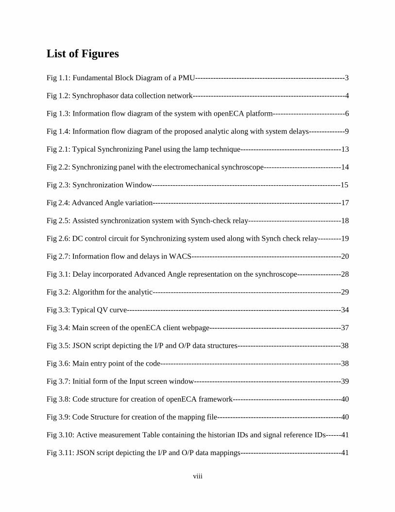
List of Figures

Fig 1.1: Fundamental Block Diagram of a PMU----------------------------------------------------------3

Fig 1.2: Synchrophasor data collection network-----------------------------------------------------------4

Fig 1.3: Information flow diagram of the system with openECA platform----------------------------6

Fig 1.4: Information flow diagram of the proposed analytic along with system delays--------------9

Fig 2.1: Typical Synchronizing Panel using the lamp technique---------------------------------------13

Fig 2.2: Synchronizing panel with the electromechanical synchroscope------------------------------14

Fig 2.3: Synchronization Window-------------------------------------------------------------------------15

Fig 2.4: Advanced Angle variation-------------------------------------------------------------------------17

Fig 2.5: Assisted synchronization system with Synch-check relay------------------------------------18

Fig 2.6: DC control circuit for Synchronizing system used along with Synch check relay---------19

Fig 2.7: Information flow and delays in WACS----------------------------------------------------------20

Fig 3.1: Delay incorporated Advanced Angle representation on the synchroscope-----------------28

Fig 3.2: Algorithm for the analytic-------------------------------------------------------------------------29

Fig 3.3: Typical QV curve-----------------------------------------------------------------------------------34

Fig 3.4: Main screen of the openECA client webpage---------------------------------------------------37

Fig 3.5: JSON script depicting the I/P and O/P data structures----------------------------------------38

Fig 3.6: Main entry point of the code----------------------------------------------------------------------38

Fig 3.7: Initial form of the Input screen window---------------------------------------------------------39

Fig 3.8: Code structure for creation of openECA framework------------------------------------------40

Fig 3.9: Code Structure for creation of the mapping file------------------------------------------------40

Fig 3.10: Active measurement Table containing the historian IDs and signal reference IDs------41

Fig 3.11: JSON script depicting the I/P and O/P data mappings---------------------------------------41

ix

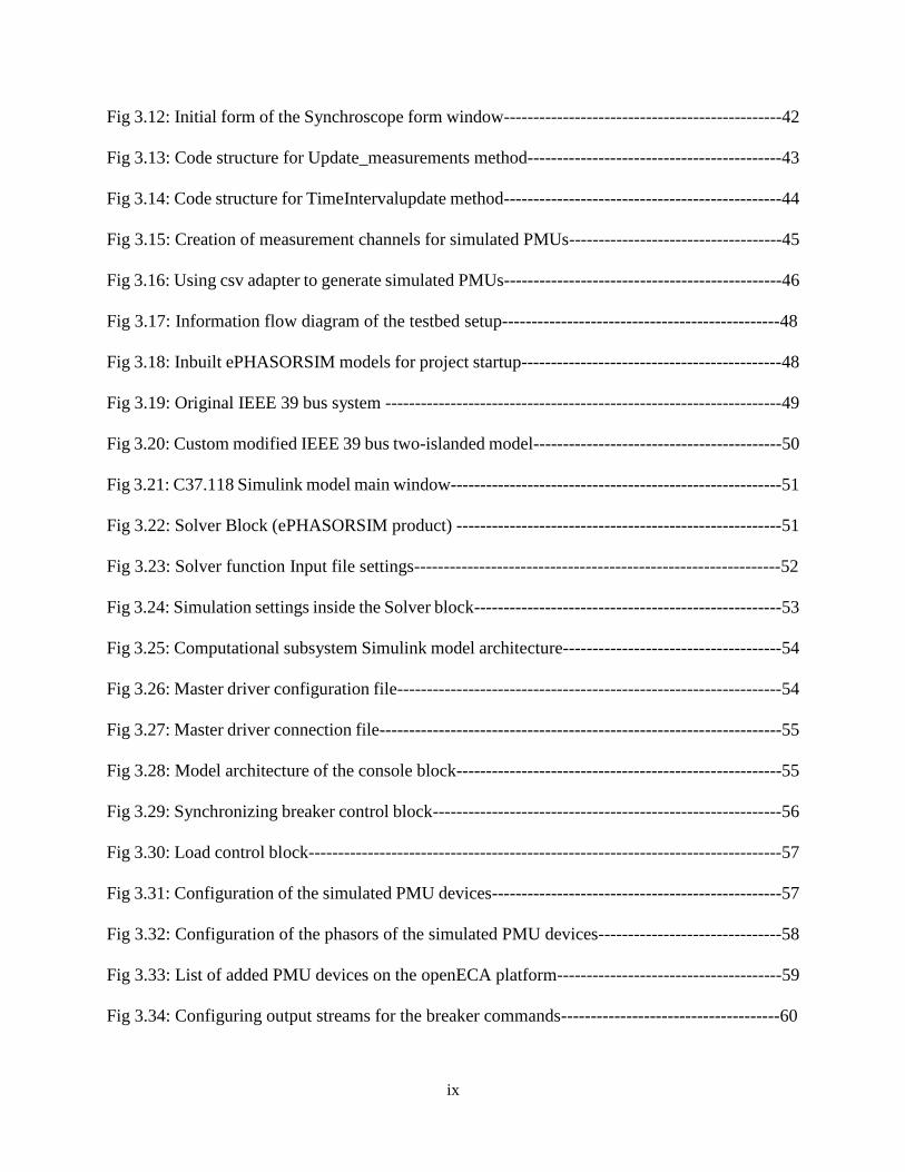
Fig 3.12: Initial form of the Synchroscope form window-----------------------------------------------42

Fig 3.13: Code structure for Update_measurements method-------------------------------------------43

Fig 3.14: Code structure for TimeIntervalupdate method-----------------------------------------------44

Fig 3.15: Creation of measurement channels for simulated PMUs------------------------------------45

Fig 3.16: Using csv adapter to generate simulated PMUs-----------------------------------------------46

Fig 3.17: Information flow diagram of the testbed setup-----------------------------------------------48

Fig 3.18: Inbuilt ePHASORSIM models for project startup--------------------------------------------48

Fig 3.19: Original IEEE 39 bus system -------------------------------------------------------------------49

Fig 3.20: Custom modified IEEE 39 bus two-islanded model------------------------------------------50

Fig 3.21: C37.118 Simulink model main window--------------------------------------------------------51

Fig 3.22: Solver Block (ePHASORSIM product) -------------------------------------------------------51

Fig 3.23: Solver function Input file settings--------------------------------------------------------------52

Fig 3.24: Simulation settings inside the Solver block----------------------------------------------------53

Fig 3.25: Computational subsystem Simulink model architecture-------------------------------------54

Fig 3.26: Master driver configuration file-----------------------------------------------------------------54

Fig 3.27: Master driver connection file--------------------------------------------------------------------55

Fig 3.28: Model architecture of the console block-------------------------------------------------------55

Fig 3.29: Synchronizing breaker control block-----------------------------------------------------------56

Fig 3.30: Load control block--------------------------------------------------------------------------------57

Fig 3.31: Configuration of the simulated PMU devices-------------------------------------------------57

Fig 3.32: Configuration of the phasors of the simulated PMU devices-------------------------------58

Fig 3.33: List of added PMU devices on the openECA platform--------------------------------------59

Fig 3.34: Configuring output streams for the breaker commands-------------------------------------60

x

Fig 4.1: RTDS simulated data plots prior and post-synchronization----------------------------------62

Fig 4.2: Synchroscope performance using RTDS simulated data--------------------------------------63

Fig 4.3: Test bench setup------------------------------------------------------------------------------------63

Fig 4.4: Trending real-time simulated measurements on openECA-----------------------------------64

Fig 4.5: Input screen window-------------------------------------------------------------------------------65

Fig 4.6: Analytic Main Window----------------------------------------------------------------------------66

Fig 4.7: Synchroscope Form Window prior synchronization-------------------------------------------66

Fig 4.8: Synchroscope Form Window post synchronization--------------------------------------------67

Fig 4.9: Voltage phase angle profile prior load control (Scenario-1) ---------------------------------69

Fig 4.10: Voltage phase angle profile post load control (Scenario-1) --------------------------------71

Fig 4.11: Voltage phase angle profile prior load control (Scenario-2) --------------------------------73

Fig 4.12: Voltage phase angle profile post load control (Scenario-2) --------------------------------74

Fig 4.13: Smoother synchronization with inclusion of load control-----------------------------------75

xi

List of Tables

Table 2.1: Typical Synch- check parameters-------------------------------------------------------------18

Table 4.1: Loads at various PQ buses of Area-1 prior load control (Scenario-1) ------------------69

Table 4.2: Inertia constants of the various generators in Area-1--------------------------------------70

Table 4.3: Loads at various PQ buses of Area-1 post load control (Scenario-1) -------------------71

Table 4.4: Loads at various PQ buses of Area-1 prior load control (Scenario-2) ------------------72

Table 4.5: Loads at various PQ buses of Area-1 post load control (Scenario-2) -------------------74

1

Chapter 1- Introduction and History

1.1 Power system restoration planning

Power system restoration planning after a wide area system blackout is crucial to improve power

system resilience. The wide area power outages and blackouts impact hugely both on the society

and economy of the country. It has been estimated that the United States alone incurs a loss of

$20–$70 billion annually [1] due to power outages. In August 2003, 50 million people lost power

for up to two days in the northeastern blackout. This event resulted in the deaths of 11 people and

a loss of an estimated $6 billion [2]. In recent past, weather-induced blackouts in the United States

like hurricane Harvey and Irma that hit Texas and Florida and hurricane Maria that hit Puerto Rico,

have been testimony about the magnanimity of the impact rendered. Puerto Rico’s apagón, or

“super blackout,” is the longest and largest major power outage in modern U.S. history. These

outage costs also are dependent upon the duration of outage and outage spread or magnitude. There

is a growing need for a more resilient grid that can recover rapidly from the impact of extended

power system blackouts following such cascading failures due to extreme weather events or

malicious attacks [4].

Power system restoration is categorized into multiple stages: system status determination, plant

preparation, generation restoration, transmission path energization, load restoration, and system

synchronization [5]. A successful restoration plan should be well designed and thoroughly studied

beforehand but still is constrained by operational and technical constraints. Some of the primary

objectives driving the restoration plan are minimizing restoration time and service interruptions,

maximizing generation capacity and load served, etc. [6].

2

1.2 Importance of synchronization process

Synchronization of small islands to establish a strong system is a crucial task during the

implementation of the abovementioned stages sequentially. Normally, an abnormal or improper

synchronization between the two islands might result in one or more of the following effects:

1. High acceleration or deceleration in the prime mover, which increases the transient

torque and might damage the rotor.

2. High transient current might flow in the windings.

3. High instant voltages might damage the insulation of the equipment.

4. Power system oscillations might occur due to the transient effect.

5. Possible operation of power system protection devices, which introduce system

outages and create additional problems.

Therefore, it is needless to state that a poor or improper synchronization among two islands might

worsen the situation even more and might lead to further delays in the power system restoration

process. Synchrophasors or PMUs (phasor measurement units) at various measuring sites have

now been able to help in this regard, as they are synchronized on a common time base. It provides

a direct measurement of system states, which has the potential to benefit power system restoration.

During the process of system restoration, PMUs can provide information for both steady state and

dynamic conditions [7]. Reports have shown that installed PMUs have made numerous significant

contributions to data acquisition during system blackout and system restoration [8, 9]. Moreover,

the deployment of PMUs has been strongly recommended by authorities after the Northeast US

and Italian blackouts in 2003 [10]. This had also led to the formation of the North American

Synchrophasor Initiative in the United States. PMUs have always attracted the power system

3

researchers due to their wide range of potential applications for system restoration and thus needs

to be studied in detail before implementing any synchrophasor-based analytics.

1.3 Synchrophasor technology and PDCs

1.3.1 Phasor Measurement Units

Integration of Intelligent Electronic Devices (IEDs) to the power system facilitates improved

visualization, control, and communication of the power system's performance. At the core, is the

development of Wide Area Measurement Systems (WAMS) and Wide Area Monitoring Protection

and Control Systems (WAMPACS) that extract consistent and time-accurate measurements from

the power system to ensure its stable, secure and economical operation [11]. The core components

of the WAMS and WAMPACS are Phasor Measurement Units (PMUs) and Phasor Data

Concentrators (PDCs). A Phasor Measurement Unit (PMU) has been defined by the IEEE as “a

device that produces synchronized phasor, Frequency, and Rate of Change of Frequency (ROCOF)

estimates from voltage and/or current signals and a time synchronizing signal.” Figure 1.1 depicts

the fundamental block diagram of a phasor measurement unit.

Fig 1.1: Fundamental Block Diagram of a PMU

These devices provide a precise and representative view of the power system as they are

synchronized to Coordinated Universal Time (UTC) through Global Positioning System (GPS)

4

signal. Therefore, these devices can provide real-time measurements recorded from different parts

of the power system.

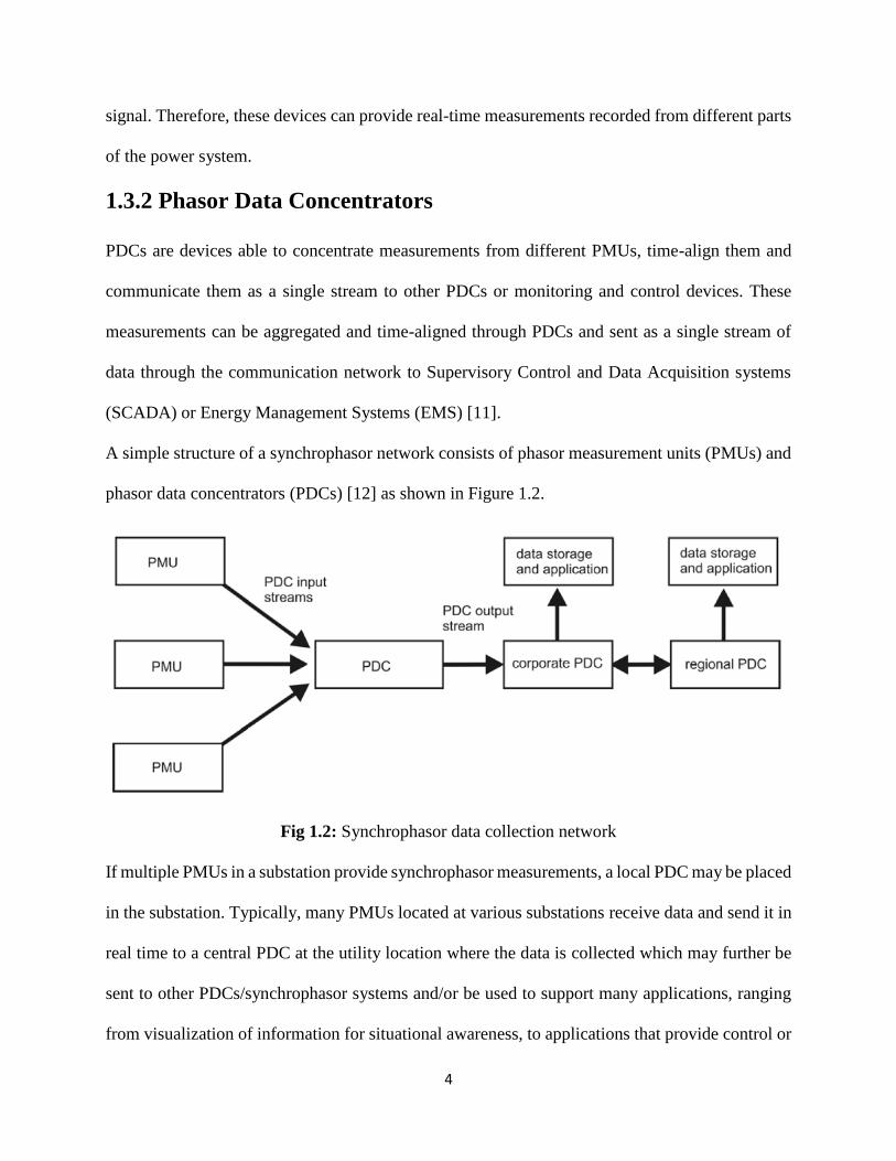
1.3.2 Phasor Data Concentrators

PDCs are devices able to concentrate measurements from different PMUs, time-align them and

communicate them as a single stream to other PDCs or monitoring and control devices. These

measurements can be aggregated and time-aligned through PDCs and sent as a single stream of

data through the communication network to Supervisory Control and Data Acquisition systems

(SCADA) or Energy Management Systems (EMS) [11].

A simple structure of a synchrophasor network consists of phasor measurement units (PMUs) and

phasor data concentrators (PDCs) [12] as shown in Figure 1.2.

Fig 1.2: Synchrophasor data collection network

If multiple PMUs in a substation provide synchrophasor measurements, a local PDC may be placed

in the substation. Typically, many PMUs located at various substations receive data and send it in

real time to a central PDC at the utility location where the data is collected which may further be

sent to other PDCs/synchrophasor systems and/or be used to support many applications, ranging

from visualization of information for situational awareness, to applications that provide control or

5

protection functionality. Many PDCs belonging to different utilities can be connected to a common

central PDC to aggregate data across the utilities, to provide an interconnection-wide snapshot of

the power grid measurements.

A PDC may perform several functions applied to synchrophasor data streams, which might depend

on the applications being served by synchrophasor data and the design of the synchrophasor

systems. Some of the vital functions of a typical PDC are enumerated as follows:

1. Data aggregation, validation, and forwarding

2. Data transfer protocol support and conversions

3. Data format and coordinate conversion

4. Phase and magnitude adjustment

5. Performance monitoring

6. Redundant and duplicate data handling

1.4 The openECA project

1.4.1 Overview

The objective of the Open and Extensible Control and Analytics (openECA) platform for

synchrophasor data project is “to develop an open source software platform that significantly

accelerates the production, use, and ongoing development of real-time decision support tools,

automated control systems, and off-line planning systems that firstly, incorporates high-fidelity

synchrophasor data and secondly, enhances system reliability while enabling the North American

Electric Reliability Corporation (NERC) operating functions of reliability coordinator,

6

transmission operator, and/or balancing authority to be executed more effectively” (Related

Links[1] in Appendix).

The openECA platform advances the production deployment of robust and high availability

synchrophasor-based software applications by creating a structured approach to the management

of real-time and historical synchrophasor measurements within a platform that can effectively

handle the most demanding of synchrophasor data system requirements. Figure 1.3 shows the

overview of the information flow of the system with the inclusion of openECA.

Fig 1.3: Information flow diagram of the system with openECA platform

Synchrophasor measurements are aggregated at the Data integration service (PDCs) as shown in

the figure and then passed on to the common analytics interface, which basically is the openECA

platform. It would act as an interface between measurements and the analytics or different

applications built by the power system researchers/developers. The openECA platform provides

some starter templates based upon a multitude of languages ranging from MATLAB, Python used

commonly in the field of power system studies to C#, C++, F# mostly in the industrial level. This

7

facilitates the developer not to focus on programming or developing the interface for their

applications, rather only focus on their respective analytics and its integration with the platform.

1.4.2 Project partners

This project is a Department of Energy-sponsored project with Grid Protection Alliance as its

principal investigator along with the following project partners:

• Dominion Virginia Power

• Virginia Tech

• Oklahoma Gas and Electric

• Southwest Power Pool

• Northwestern Energy

• Bonneville Power Administration

• T&D Consulting Engineers

1.4.3 Possible benefits of the project

1.4.3.1 Value to industry

1. Lowers cost of addition of new production analytic tools.

2. Simplified end-to-end configuration and change management.

3. Improved availability of phasor data with greater visibility of phasor data quality.

4. Robust scalable solution to support phasor data infrastructure of any size.

5. Complements current phasor data architecture and supports integration with other data

sources such as SCADA.

8

1.4.3.2Value to research community

1. Allows research community to focus on development of new techniques and tools and

not on learning how to build information interfaces.

2. Removes barriers to installation of newly developed research tools in production

software environments.

1.5 Motivation

As a part of the openECA project, numerous synchrophasor-based analytics were to be developed

under the collaboration of Virginia Tech and Dominion Energy Virginia. One of the focus was to

use synchrophasor technology for faster power system restoration. As discussed earlier,

synchronization of islands is a crucial stage of restoration process especially during blackstart.

Normally, the synchronization process is monitored and carried out using a synchroscope at the

substation level. A traditional synchroscope is basically a physical piece of hardware used to

synchronize two buses or nodes with different frequencies. The restoration procedures generally

are planned based on blackstart studies and simulations which are executed earlier and thus follow

a predetermined path. Although this path may be pre-determined, one thing that should be

considered in the actual implementation is that not all substations are manned and equipped with

a synchroscope. This requires the physical transfer of the synchroscope device from one substation

to the desired location. This additional activity costs the utility in terms of money and time and

significantly limits the flexibility to establish and implement system restoration strategies.

Furthermore, the synchronization process is mainly monitored and operated under the surveillance

of the experienced substation crews with the help of the synchroscope. Therefore, any technical or

human error might lead to unsuccessful or improper synchronization of the two islands. Moreover,

as the substations have no control effect on the island’s frequency and voltage, carrying out such

9

a crucial task at the substation level might not provide a bigger picture for controlling or even

predicting after synchronization transients /power swings in the system.

However, with the advent of phasor measurement units providing time synchronized

synchrophasor data, the synchroscope functionality can now be realized at a centralized remote

control platform, usually the control room of the specified utility. Obviously, to achieve such

functionality at a remote centralized location, the primary challenge is to overcome the various

delays associated with the wide area measurement system. Figure 1.4 depicts the overview of the

proposed analytic along with the various delays associated with the system highlighted in red

boxes.

Fig 1.4: Information flow diagram of the proposed analytic along with system delays.

Once these delays and their respective variances are determined, a predicted time instant for

closing the synchronizing breaker can be calculated to achieve time synchronized breaker closing

action at the substation leading to successful synchronization. This thesis presents a technique to

implement a modified synchroscope application based upon the openECA platform to be used at

10

a remote centralized location (hereafter referred to as PMU synchroscope throughout the document

for better understanding). The application would predict a particular time instant to initiate the

synchronizing breaker close command, overcoming the delays, which might have hindered a

proper synchronization activity if not included. Apart from initiating proper breaker command

signals, it also raises alarms and annunciations for the convenience of the operators/users to bring

the measurements between the two buses within acceptable tolerance limits. The tolerance limits

can also be defined by the user/utility depending upon the system parameters and operating

conditions.

The methods adopted by the user to achieve these desired results are completely subjected to the

discretion of the user/utility. However, as the main focus of this particular work is on bulk power

system restoration during which the utility has control over load changes to a flexible extent, this

thesis has also presented a technique for an integrated load control technique based upon voltage

sensitivities of the load buses in one of the islands in order to bring it closer to the frequency of

the reference island or grid. This simply acts as a demonstration of how various techniques can be

embedded with this application if required in the future.

The rest of the thesis is organized in the following way:

Chapter 2: Traditional synchroscopes and load control techniques

This chapter presents a literature review of the past work done on synchroscopes, explaining its

fundamental functionality. It also discusses the various delay assessment and modeling carried out

in the past, which would help us later in the implementation stage of the application. Lastly, it

discusses the load control technique finally adopted to be implemented in the analytic.

11

Chapter 3: Algorithm Formulation and Test Setup Implementation.

This chapter presents with the algorithm developed based on the literature review and findings in

chapter-2. Based upon this algorithm, the implementation of the application’s code structure is

discussed elaborately. Once the standalone application is developed, the chapter then discusses the

various test setup configurations required to validate and demonstrate the analytic developed along

with its compatibility with the openECA platform.

Chapter 4: Test Scenarios and Results.

This chapter provides the results of the testing of the PMU Synchroscope based upon the various

test setups developed in chapter-3. Additionally, the performance of the load control technique

adopted is also depicted with observations for the same.

Chapter5: Conclusion and Future work.

The chapter concludes the thesis and summarizes the work completed along with remarks. It also

discusses the future work related to this application and recommends several other ideas for

expansion of the topic.

12

Chapter-2: Traditional synchroscopes and load

control techniques

2.1 Traditional synchroscopes and early work

Synchronization is the process of matching a source (might be a generator or a small islanded area)

with a large existing power system, making it possible to operate these systems in parallel. When

two segments of a grid are disconnected, these segments cannot exchange power and share load

again until the systems are synchronized and paralleled back together. The synchronization process

is usually achieved by an operator, who can synchronize manually or use one of the latest, state-

of-the-art automatic synchroscopes (ANSI/IEEE device 25A) [1] and sync-check relays

(ANSI/IEEE device 25) to automate closing [13]. The following power system quantities of the

incoming source must match the same quantities of the existing or the reference system:

• Phase sequence

• Voltage amplitude

• Frequency

• Phase angle

2.1.1 Traditional technique

One of the oldest techniques of determining if the incoming voltage is in phase with the running

voltage is using two lamps connected in series across the phase wires of the incoming and running

or reference voltage signals [14] as shown in figure 2.1. The figure below shows a typical

synchronizing panel for a generator with two synchronizing breakers. SS1 is the synchronizing

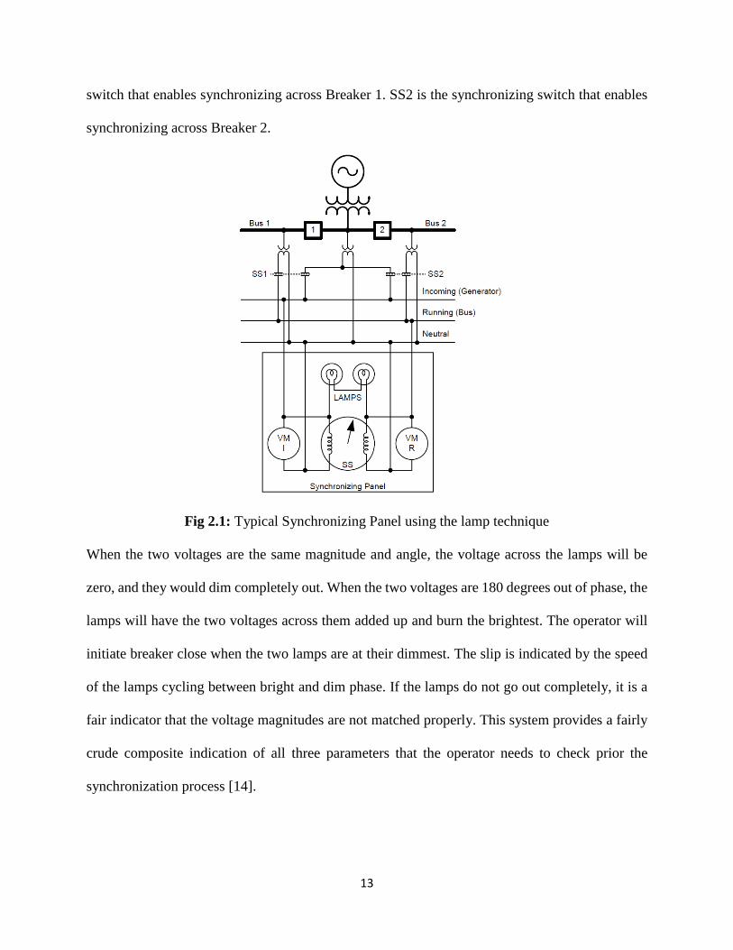
13

switch that enables synchronizing across Breaker 1. SS2 is the synchronizing switch that enables

synchronizing across Breaker 2.

Fig 2.1: Typical Synchronizing Panel using the lamp technique

When the two voltages are the same magnitude and angle, the voltage across the lamps will be

zero, and they would dim completely out. When the two voltages are 180 degrees out of phase, the

lamps will have the two voltages across them added up and burn the brightest. The operator will

initiate breaker close when the two lamps are at their dimmest. The slip is indicated by the speed

of the lamps cycling between bright and dim phase. If the lamps do not go out completely, it is a

fair indicator that the voltage magnitudes are not matched properly. This system provides a fairly

crude composite indication of all three parameters that the operator needs to check prior the

synchronization process [14].

14

2.1.2 Electromechanical Synchroscope

However to improve visualization of the actual angle between the incoming and running voltages

and to improve the response of the operator to synchronize properly, a synchroscope is used in

modern synchronizing panels. Figure 2.2 shows an example of an electromechanical

synchroscope. The traditional synchroscope does not indicate voltage magnitude difference, so

voltmeters for incoming voltage and running voltage are often included. Additionally, frequency

meters are sometimes included on the synchronizing panel.

Fig 2.2: Synchronizing panel with the electromechanical synchroscope

As seen in the figure, the synchroscope indicates the phase angle difference so that when the two

voltages are in phase, the pointer points straight up (12 o’clock position) representing zero degrees.

In other words, the 12 o’clock position is the reference bus phasor position and the rotating pointer

represents the incoming bus phase angle (Vin) w.r.t to the reference bus. Therefore, the operator

initiates closing the breaker when the phase angle difference between the incoming voltage and

the system voltage is close to 0 degrees. When the incoming phasor is running faster than the

reference phasor, the pointer rotates in the clockwise direction and vice versa. The revolutions per

minute (rpm) of the synchroscope indicates the slip. For example, a synchroscope rotating at 3 rpm

equates to 0.05 Hz slip. The operator can determine whether to raise or lower the incoming bus

15

voltage or frequency based on these indications. The acceptable tolerance limits constitute the

synchronization window [13] on the synchroscope device. Figure 2.3 depicts the synchronization

window which displays the bus voltage Vref (running or reference bus), on the vertical axis.

Acceptable difference in voltage amplitude limit(∆V), acceptable phase angle (slip-angle θ)

window, in degrees and the acceptable slip frequency, ∆f, in hertz are specified differently for

different scenarios.

Fig 2.3: Synchronization Window

For synchronizing generators with the grid, IEEE Standards C50.12 and C50.13 provide

specifications for the construction of cylindrical-rotor and salient-pole synchronous generators,

respectively. The limits for both types of generators are specified as:

• Angle ±10 degrees.

• Voltage 0 to +5 percent.

• Slip ±0.067 Hz.

Narrower tolerance limits produce less system disturbance or power swings and machine damage

post synchronization (otherwise known as "softer" synchronization). On the other hand, much

Vref

Vin

16

wider tolerance limits allow synchronization to be achieved faster but produce more system

disturbance and transients (otherwise known as "harder" synchronization) [13].

The various factors to be considered in deciding these are

• Acceptable power restoration time.

• System loading and operating conditions which depicts its criticality

• Economic aspects regarding damages to the various equipment in the region.

A proper synchronization activity needs to consider these as well as others that are unique to the

system. Although it might vary for various systems and the limits might be wider for a two-island

synchronization, the point put forth is that the operator would bring the respective quantities as

close to each other within the specified limits to ensure a smoother synchronization.

2.1.3 Automatic Synchronizers

Apart from the manual synchronizers, automatic synchronizers (ANSI/IEEE device 25A) are also

used primarily for generator synchronization which automatically tries to send the control signals

for the governor and automatic speed regulator (AVR) to control (both raise and lower) the output

voltage and speed of the generator and to bring it within acceptable limits (within the

synchronization window). Traditionally, in the case of manual synchronizer, a good operator

judges how fast the phase angle difference is catching up and hence, energizes the breaker close

coil accordingly in advance to account for the closing mechanism delay of the synchronizing

breaker in such a fashion that the main contacts make as close to a zero-degree angle difference as

possible at the time of actual closing in the field . However, the modern automatic synchroscopes

measure the slip and calculates what is termed as an advanced angle, which in simple terms is the

actual instant to energize the close coil to compensate for the breaker close mechanism delay [14].

The slip-compensated advanced angle is calculated using the following equation:

17

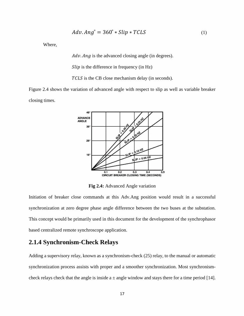
𝐴𝑑𝑣. 𝐴𝑛𝑔 ͦ = 360 ͦ ∗ 𝑆𝑙𝑖𝑝 ∗ 𝑇𝐶𝐿𝑆 (1)

Where,

𝐴𝑑𝑣. 𝐴𝑛𝑔 is the advanced closing angle (in degrees).

𝑆𝑙𝑖𝑝 is the difference in frequency (in Hz)

𝑇𝐶𝐿𝑆 is the CB close mechanism delay (in seconds).

Figure 2.4 shows the variation of advanced angle with respect to slip as well as variable breaker

closing times.

Fig 2.4: Advanced Angle variation

Initiation of breaker close commands at this Adv.Ang position would result in a successful

synchronization at zero degree phase angle difference between the two buses at the substation.

This concept would be primarily used in this document for the development of the synchrophasor

based centralized remote synchroscope application.

2.1.4 Synchronism-Check Relays

Adding a supervisory relay, known as a synchronism-check (25) relay, to the manual or automatic

synchronization process assists with proper and a smoother synchronization. Most synchronism-

check relays check that the angle is inside a ± angle window and stays there for a time period [14].

18

The relay cannot control or bring the parameters within acceptable limits and has to be controlled

manually or with the help of automatic control. The supervisory relay simply enforces a

synchronization window for safe conditions that must be in place before the synchronizing breaker

can be closed [13] as shown in figure 2.5.

Fig 2.5: Assisted synchronization system with Synch-check relay

The sync-check relay compares the voltage difference, slip frequency, and phase angle (slip)

differences between the incoming bus and the reference bus. Typical setting ranges for these

parameters are depicted in the table below.

Parameters Typical Value

Voltage difference ± 4V-8V secondary

Phase (slip) angle -25 ͦ to +25 ͦ

Frequency slip ± 0.1 Hz

Table 2.1: Typical Synch- check parameters

The supervisory 25 relay does not allow a circuit breaker closure until all of these parameters are

satisfied and thus prevents the synchronizing breaker to close out of phase. The sync-check relay

output contacts are in series with the operator control switch. Circuit breaker closing occurs only

when either the operator manually closes the switch or automatically if an automatic synchronizer

is used, and the supervisory relay contacts are closed. The DC control circuit is shown in figure

2.6.

19

Fig 2.6: DC control circuit for Synchronizing system used along with Synch check relay

All these considerations have to be taken into factor while designing a remote synchroscope using

synchrophasors. [14] discusses a synchrophasor based synchroscope (PDC synchroscope) in which

a dedicated computer running synchrophasor data concentrator (PDC) software can receive

streaming data from the various microprocessor-based relays applied for protection and control of

the synchronizing breakers. However, it talks about low latency constraint for such a soft

synchroscope developed. It also does not incorporate the inclusion of different latency issues in

the wide area measurement systems in such an application. To develop a fully functioning generic

synchrophasor based centralized remote synchroscope, the different network delays in the system

must be considered which are discussed in the following section.

2.2 Wide Area Control systems (WACS)

Wide area control systems use the wide area PMU data to control the various electrical and

electronic components in the power systems. The application which is developed in this thesis

comes within the category of Wide area Control systems. As discussed earlier, the performance of

such applications rely upon the communication delays as well as the operational delays present in

the WACS and hence, must be predetermined beforehand. Figure 2.7 depicts the information flow

and various delays associated with the WACS.

20

Fig 2.7: Information flow and delays in WACS

As shown in the figure, the main components are PMUs, wide area networked control services

(WNCS) and networked control units (NCU), acting as sensors, controllers, and actuators

respectively.

2.2.1 Delays associated with WACS

All the delays associated with the system are categorized into five parts [17]:

1. Measurement delay (tmeas): It encompasses the signal transferring delay of CTs and PTs,

synchronized sampling delay, phasor calculation delay and data packaging and sending delay.

Apart from these, the response time of the digital filters in the PMUs increases measurement

delays. However, the value is in the order of 10-15 milliseconds and can be termed as constant

for our application due to minor variances[17].

2. Data uplink delay (tup): It represents the delay to transmit data packets from PMUs to the

WNCS through the communication network and the various communication devices such as

communication servers and firewalls at various substations.

21

3. Synchronization and calculation delay (tcal): It represents the time required to perform the tasks

in WNCS such as receiving and resolving the PMU data packets, synchronizing the data from

different PMUs, calculating the control signals, and sending the control data. This delay can be

calculated based upon the computational efficiency of the user system.

4. Data downlink delay (tdown): It is the delay to transmit control data from the WNCS to NCUs.

This normally is same at the data uplink delay but might differ if data has to pass through

SCADA protocol instead of the faster C37.118 protocol.

5. Controller action delay (tctrl): It includes the delay required for the NCU to receive and resolve

the control data packets, and then send the control orders to the breakers. The breaker closing

time is also included in this category for simplicity.

Whereas tup and tdown delays constitute the communication delays, tmeas, tcal and tctrl constitute the

operational delays. As we have discussed above the operational delays are deterministic and can

be termed constant for our application. In regards to the communication delays, the upstream

delays tup can usually be derived in our case based upon the difference in time stamp values of the

measurements when compared with the time instant it is received by the application. Therefore,

the user system at the control center needs to be GPS synchronized with a high precision clock.

However, the downstream delay tdown might differ from the tup if different protocols are used for

sending the breaker command signals. Hereafter, our discussion would be mainly focused on the

modeling of this downstream delay.

2.2.2 Downstream Communication Delays

The results in [16] calculate the communication latency via different media in the WAMS of the

US Pacific Northwest power system: the latency of the fiber optic digital communication was

around 38 ms, while the latency using modems over analog microwave channels was over 80 ms.

22

The communication delay in general varies from a few milliseconds to even hundreds of

milliseconds and depends upon various factors, which is discussed in the following sections. The

author in [17] proposes an affine model for the communication delays. The communication delay

consists of the following delays:

1. Propagation delay (α): It is the time required to transmit a packet from the sending port to the

receiving port through a particular medium. The delay α is determined by the transmission media

and distance, but not the bandwidth. During the case of synchronization at a particular substation,

both these terms are invariant, and thus propagation delay in our case can be termed as a constant.

2. The serial delay (β): It is the time required to synchronize the bits of a data packet at a certain

transmission speed. The delay is proportional to the data packet size (L) and inversely

proportional to the bandwidth of the link (R) [18].

β =𝐿

𝑅 (2)

3. The routing delay (γ): It is the total time that a packet spends at a node, including both the

waiting and service time, and is related to the network traffic [17]. As during synchronization

procedure, light network traffic would be warranted for smooth functionality, the delay γ can be

ignored.

4. The terminal delay (λ): It includes the delays caused due to physical firewalls and

communication servers on each side of the channel. These delays can also be treated as a constant.

So for j nodes and k links in a channel for the downstream communication, then tdown can be written

as:

𝑡𝑑𝑜𝑤𝑛 = ∑ α𝑖𝑘𝑖=1 + ∑ β𝑖

𝑗𝑖=1 + ∑ γ𝑖

𝑗𝑖=1 + 2𝜆 (3)

23

As discussed above, the propagation and terminal delays can be clubbed together as a constant and

routing delay can be neglected, the final equation defining the affine evaluation model(AEM) for

communication delays, varying linearly as the size of the data packets for light network conditions

is represented as:

𝑡𝑑𝑜𝑤𝑛 = 𝑇𝑜 +𝐿

𝑅 (4)

Where,

𝑇𝑜 = ∑ α𝑖𝑘𝑖=1 + 2𝜆 (5)

The above defined AEM would be used to model the downstream communication delays. Firstly,

as discussed in [17], several groups of measurement data for tdown are taken with different L in a

channel. Second, the average of each group of tdown is calculated. Finally, the parameters To and R

of AEM are calculated by linear fitting. The measurement method of these tdown is separately

explained in the next chapter.

2.3 Load Control Technique

The literature review for the implementation of the PMU synchroscope has been discussed in the

earlier sections. However, the synchroscope to be designed does not have the capability to

automatically change the voltage and frequency of the island under observation. Conventional

synchroscopes send control signals for the governor and AVR of the generator to bring the

parameters within the limit. As the PMU synchroscope application deals with island

synchronization in general (which also can be used for generator synchronization), control

schemes have been out of the context for this project as each scenario would be different and has

to be tailor-made for control of frequency and voltage of the power source (single generator or an

island) to be synchronized. Therefore, to demonstrate a generic functionality of control measures,

24

an add-on functionality is included in this thesis work, as a representation of the control measures,

which might be used by the operator in the utility. Although the utility might have other control

measures to achieve the same, the following work intends to show how a generic system-wide

control measure can be used in conjunction to the PMU synchroscope to achieve smoother

synchronization with minimal power swings after synchronization. Moreover, as voltage control

methods are being developed as a part of several separate analytics in the openECA project, the

main focus would be frequency control of the island which must consider both frequency and

voltage measurements for better analysis. One of the important assumptions made in this context

is that even if the PMU synchroscope developed can be used for either black start or normal

synchronization procedure, the main focus of the analytic or motivation was for bulk power system

restoration. Therefore, it would be safe to assume that during this situation, the utility has huge

control on the load and can be modified to a larger extent at the time of blackstart operation or load

rich islanded system. This might not be true for a normal synchronization procedure, and the utility

might use generation control to achieve this. However as stated earlier, generator governor control

is tailor made for separate generators and therefore, the add-on functionality depicted in this

document focusses on how a generic control method such as a load control technique can be

integrated with the PMU synchroscope.

Based on the above assumption, a technique stated in [21] is discussed and implemented in the

document. Although the technique stated in [21] deals with load shedding, the main reason to adopt

this technique is that it focusses on a load shedding scheme which not only corrects the system

frequency but also improves the voltage profile throughout any system which can be modified to

meet the requirements of the synchroscope application. The main purpose of this method is that it

considers the rate of change of frequency and the voltage sensitivities before implementing the

25

actual load shedding scheme which is beneficial for the situation at hand. The scheme is simple

and does not involve complicated calculations. It has proved to be successful in restoring the

frequency within its pre-defined limits and henceforth would be discussed in the next chapter in a

modified fashion to suit our requirements and not simply on load shedding. A quick summary of

the method is stated as follows.

The first step is the measurement stage which collects the voltage values along with the rate of

change of frequency values at each bus. When a disturbance causes a deviation in frequency or a

change in bus voltage or both, it is recorded, and the magnitude of the disturbance is estimated

using the power swing equation. This determines the amount of load to be shed finally. Once, the

quantity of load to be shed is decided, the buses are ranked according to their dV/dt values. This

ranking decides the order in which load will be shed. Therefore, the bus where the voltage is

declining at a faster rate has a higher dV/dt value and is ranked at a higher position. Once the order

of the shedding is decided the next stage calculates how much load needs to be shed from each

load bus. This is decided by a formula based on the voltage sensitivities [21] (otherwise called as

V-Q sensitivity) based upon the V-Q curve analysis. System planners conduct numerous studies

using the V-Q curve to determine the amount of load that needs to be shed to retain voltage

stability. Finally, load shedding may be manual or automatic. However, for the sake of the work

stated in this document, this particular load shedding technique has been modified and now applied

to both load increase as well as load shedding to bring the frequency of the incoming island close

to the running or reference island which is discussed in the algorithm section of chapter-3.

26

Chapter-3: Algorithm Formulation and Test Setup

Implementation

3.1 Algorithm Formulation

3.1.1 Calculation of system delays

As discussed in the previous chapter, the various delays in the system are constant and can be

calculated easily except the communication delays. However, we can calculate the actual

communication delays associated with the system beforehand using an affine evaluation model

(AEM) using Eqn. 4. For calculation of those parameters and measurement of the communication

delays, the method suggested in [17] can be implemented as follows:

Step-1: Data packets conforming to actual PMU data sizes are constructed. Then the sending

server, which is at the same port as the WAMS server in the control center, sends the

constructed data packets to the receiving server, which is at the same port as the PMU.

Step-2: The receiving server returns the data packets immediately after receiving the packets.

The sending server times the sending and receiving operations by a local timer.

Step-3: The time intervals are calculated which is twice the communication delays. The statistics

of the communication delays can be obtained from the various groups of measurement

tests.

In an alternative method, timestamped data packets are sent from the control server (in our case

the openECA instance at the control center), and another openECA instance at the substation level

receives these data packets. Measuring the difference in timestamps of the received data packets

with the coordinated universal time, we can measure the average value of the downstream

27

communication delays, which would be then fed into the application to calculate the advanced

angle as discussed earlier. It should be noted that the variances in the communication delays are

relatively insignificant to affect the functionality of the synchroscope and hence are neglected,

which is discussed in the next section.

3.1.2 Advanced Angle calculation

Once the synchronization path is adopted, and the downstream delays in that particular path are

estimated, the mean value of the delay can be fed to the core algorithm of the analytic. To include

this delay in the system, we use the concept of advanced angle as discussed in the earlier chapter

as used for automatic synchronizers, which is the representation of the movement of the voltage

phasor of the incoming bus with reference to the voltage phasor of the reference bus in regards to

the delays associated. In other words, it provides a predicted angle or position for the rotating

phasor hand of the synchroscope if these delays are considered and the all the other parameters of

the system are kept constant or stable.

The advanced angle is now modified and is a function of the cumulative delays (which includes

all the upstream as well downstream delays in addition to the breaker closing time) and the

associated slip in frequency between the two buses to be synchronized. It is represented by the

equation as shown below:

𝐴𝑑𝑣. 𝐴𝑛𝑔 ͦ = 360 ͦ ∗ 𝑆𝑙𝑖𝑝 ∗ 𝐶𝑢𝑚𝑢𝑙𝑎𝑡𝑖𝑣𝑒 𝐷𝑒𝑙𝑎𝑦𝑠 (6)

𝐶𝑢𝑚𝑢𝑙𝑎𝑡𝑖𝑣𝑒 𝐷𝑒𝑙𝑎𝑦𝑠 = 𝑜𝑝𝑒𝑟𝑎𝑡𝑖𝑜𝑛𝑎𝑙 𝑑𝑒𝑙𝑎𝑦𝑠 + 𝑡𝑢𝑝 + 𝑡𝑑𝑜𝑤𝑛 + 𝑇𝐶𝐿𝑆 (7)

Where,

𝐴𝑑𝑣. 𝐴𝑛𝑔 is the advanced closing angle (in degrees).

𝑇𝐶𝐿𝑆 is the CB close mechanism delay (in seconds).

28

𝑡𝑢𝑝 is the upstream delay (in seconds).

𝑡𝑑𝑜𝑤𝑛 is the downstream delay (in seconds).

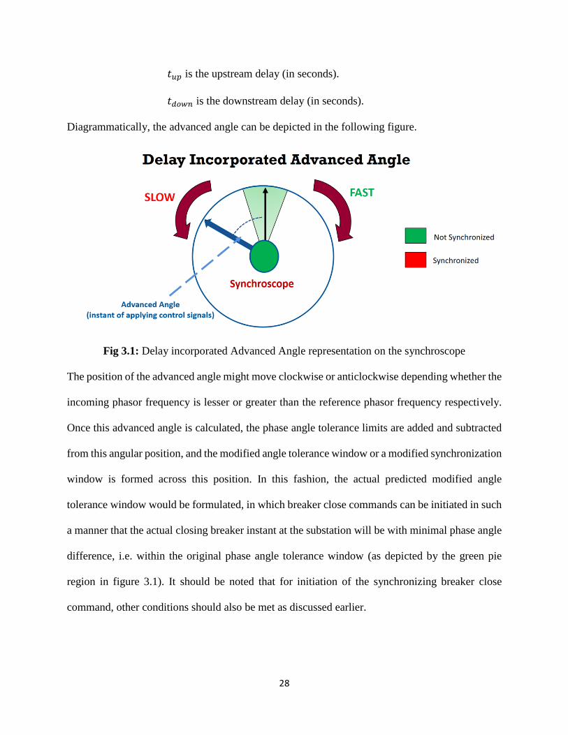
Diagrammatically, the advanced angle can be depicted in the following figure.

Fig 3.1: Delay incorporated Advanced Angle representation on the synchroscope

The position of the advanced angle might move clockwise or anticlockwise depending whether the

incoming phasor frequency is lesser or greater than the reference phasor frequency respectively.

Once this advanced angle is calculated, the phase angle tolerance limits are added and subtracted

from this angular position, and the modified angle tolerance window or a modified synchronization

window is formed across this position. In this fashion, the actual predicted modified angle

tolerance window would be formulated, in which breaker close commands can be initiated in such

a manner that the actual closing breaker instant at the substation will be with minimal phase angle

difference, i.e. within the original phase angle tolerance window (as depicted by the green pie

region in figure 3.1). It should be noted that for initiation of the synchronizing breaker close

command, other conditions should also be met as discussed earlier.

29

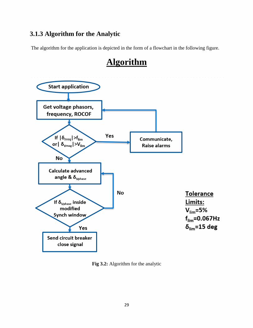
3.1.3 Algorithm for the Analytic

The algorithm for the application is depicted in the form of a flowchart in the following figure.

Algorithm

Fig 3.2: Algorithm for the analytic

30

The algorithm can be stated as follows:

1. The synchrophasor measurements of the two buses to be synchronized, which include the

voltage phasor measurements as well as frequency and rate of change of frequency (ROCOF) are

streamed into the application.

2. If the difference in voltage magnitude and frequency measurements between the two buses

is beyond the user-specified limits, proper alarms and annunciations are raised and communicated

to the user.

3. Once the user takes the necessary actions and brings the measurements within acceptable

tolerance limits of each other, the voltage phase angle difference is checked continuously to lie

inside the modified synchronization window calculated based upon the advanced angle calculated

and the phase angle tolerance limits.

4. At this stage, breaker close command is initiated either manually by the user or automatically

generated by the analytic at the advanced angle angular position to finally close the breaker at zero

degrees phase angle difference after the cumulative delays have elapsed.

3.1.4 Load control technique based upon voltage sensitivity

As discussed in the earlier chapter, the load control technique which is being integrated into this

project as a part of a demonstration of how frequency control measures can be incorporated along

with the analytic, is being derived from the load shedding technique provided in [21].

The whole algorithm is divided into three steps:

Step-1: Calculation of total load change

The main motive is to bring the incoming phasor frequency (fincoming) close to the reference phasor

frequency, and thus all the control measures are restricted to the incoming island and its generators

and loads. The first step is to estimate the total amount of load to be modified for achieving this

31

desired frequency (freference). This can be calculated using the swing equation. Normally, the swing

equation for a particular generator can be written as follows:

2𝐻

𝜔𝑠

𝑑2𝛿

𝑑𝑡2 = 𝑃𝑚 − 𝑃𝑒 (8)

It can be modified and written as,

⇒ 2𝐻

𝑓0

𝑑𝑓

𝑑𝑡= 𝑃𝑚 − 𝑃𝑒 = 𝑃𝑑𝑖𝑓𝑓 (9)

where,

H is the inertia constant of the generator.

𝛿 is the internal angle of the generator otherwise known as load/power angle.

𝜔𝑠 is the synchronous angular velocity of the generator.

𝑓0 is the nominal frequency of the system.

𝑃𝑚 is the mechanical input power to the generator.

𝑃𝑒 is the electrical output power of the generator.

This equation is valid for a single generator. For a multi-machine system in an island which

swings together, the swing equations can be combined. Such machines are called as coherent

generators. The equivalent inertia constants, mechanical input and electrical output power to the

overall system (consisting of n generators) can be written as:

𝐻𝑒𝑞 = ∑ 𝐻𝑖𝑛𝑖=1 (10)

𝑃𝑚𝑒𝑞 = ∑ 𝑃𝑚𝑖𝑛𝑖=1 (11)

𝑃𝑒𝑒𝑞 = ∑ 𝑃𝑒𝑖𝑛𝑖=1 (12)

Where,

𝐻𝑒𝑞 is the equivalent inertia constant of the whole island containing n generators.

32

𝑃𝑚𝑒𝑞 is the equivalent mechanical input power for the multi-machine islanded system.

𝑃𝑒𝑒𝑞 is the equivalent electrical output power or load for the multi-machine islanded

system.

So,

𝑃𝑑𝑖𝑓𝑓𝑒𝑞 = 𝑃𝑚𝑒𝑞 − 𝑃𝑒𝑒𝑞 (13)

𝑃𝑑𝑖𝑓𝑓𝑒𝑞 is the total modification in the load consumption required to achieve the desired

frequency within a stipulated time period tdiff as decided by the utility based upon the convenience

and availability of loads.

Therefore, a derivation from the modified swing equation for the multi-machine system can be

written as:

2𝐻𝑒𝑞

𝑓0

∆𝑓

∆𝑡= 𝑃𝑑𝑖𝑓𝑓𝑒𝑞 (14)

Where,

∆𝑓

∆𝑡= (

𝑓𝑖𝑛𝑐𝑜𝑚𝑖𝑛𝑔−𝑓𝑟𝑒𝑓𝑒𝑟𝑒𝑛𝑐𝑒

𝑡𝑑𝑖𝑓𝑓) (15)

The time tdiff and thus the necessary average rate of change of frequency needed to achieve the

desired frequency after the predefined overall load change can be decided by the utility depending

upon restoration capability. For achieving a larger change in frequency within a stipulated time,

the rate of change of frequency and hence the load change should be higher and vice versa. In this

way, the total load change required in the islanded system can be calculated.

Step-2: Ranking the load buses for modifying load.

Now once, we have the total load change desired, the various load buses are ranked in order of

priority to have their share of load changed. This was carried out on the basis of dV/dt values in

33

the original paper in case of a disturbance. However, for the sake of this project, the priority would

be based on sheer voltage magnitudes at the load buses. In other words, if the overall load is to be

shed at each load bus, the bus with the lowest voltage magnitude is given priority first which makes

sense as the voltage profile of the bus with the lowest voltage magnitude should be alleviated

sooner. On the other hand, if the overall load is to be increased at each load bus, the bus with the

highest voltage magnitude is chosen first for the addition of load followed by others. However, the

user in the utility might follow this scheme or might not depending upon convenience and load

availability conditions at that particular time.

Step-3: Allocating the % share of load change for each load bus.

Now, once the overall load change required for matching the frequencies of the two islands along

with a ranking of the load buses is calculated, the next task is to allocate the % share of load change

for each load bus within the island. This is done based on the voltage sensitivity factor of each

load bus which is calculated based on the QV analysis. Now the QV analysis is carried out in the

following manner.

The equations for active and reactive power injections at a particular bus (i) are formulated as:

` 𝑃𝑖 = ∑ |𝑉𝑖||𝑉𝑗||𝑌𝑖𝑗|cos (𝛿𝑖𝑗 − 𝜃𝑖𝑗)𝑛𝑗=1 (16)

𝑄𝑖 = ∑ |𝑉𝑖||𝑉𝑗||𝑌𝑖𝑗|sin (𝛿𝑖𝑗 − 𝜃𝑖𝑗)𝑛𝑗=1 (17)

QV analysis provides the relation between the change in voltage at a bus dependent upon the

reactive power change at that particular bus. Therefore taking the derivative of Qi with respect to

Vi, we get

𝑑𝑄𝑖

𝑑𝑉𝑖= ∑ |𝑉𝑗||𝑌𝑖𝑗|sin (𝛿𝑖𝑗 − 𝜃𝑖𝑗)𝑛

𝑗=1 (18)

34

This is termed as the voltage sensitivity of V-Q sensitivity of the bus. Now, if we look into a typical

QV curve as shown in figure 3.3, the knee point (voltage collapse point) of the plot denotes that

the system is in a critical situation and is unstable beyond that point. As the knee point is

approached, the dQ/dV values become smaller and close to zero. Thus, a system bordering on

instability will have a small value of the slope at the knee point and having a high positive value

of slope and away from the knee point would indicate high stability.

Fig 3.3: Typical QV curve

Therefore, a higher amount of load shed is warranted for the buses having lesser voltage sensitivity

value and vice versa for load increase case. In other words, for load shed or decrease case:

𝑑𝑄𝑖

𝑑𝑉𝑖 𝑖𝑠 𝑖𝑛𝑣𝑒𝑟𝑠𝑒𝑙𝑦 𝑝𝑟𝑜𝑝𝑜𝑟𝑡𝑖𝑜𝑛𝑎𝑙 𝑡𝑜 𝑡ℎ𝑒 𝑙𝑜𝑎𝑑 𝑠ℎ𝑒𝑑

or,

𝑑𝑉𝑖

𝑑𝑄𝑖 𝑖𝑠 𝑑𝑖𝑟𝑒𝑐𝑡𝑙𝑦 𝑝𝑟𝑜𝑝𝑜𝑟𝑡𝑖𝑜𝑛𝑎𝑙 𝑡𝑜 𝑡ℎ𝑒 𝑙𝑜𝑎𝑑 𝑠ℎ𝑒𝑑

Now, the load shed at each bus is a fraction of the total load required to be shed to maintain the

power balance. This fraction of the load at each bus is proportional to the fraction of the dV/dQ

value at each bus with respect to the sum of all dV/dQ values calculated for all buses.

Knee point

35

Thus, the load change at each load bus in the load decrement scenario is represented as:

𝐿𝑜𝑎𝑑𝑐ℎ𝑎𝑛𝑔𝑒𝑖 =

𝑑𝑉𝑖𝑑𝑄𝑖

∑𝑑𝑉𝑗

𝑑𝑄𝑗

𝑛𝑗=1

∗ 𝑃𝑑𝑖𝑓𝑓𝑒𝑞 (19)

Similarly, for the load increment case,

𝐿𝑜𝑎𝑑𝑐ℎ𝑎𝑛𝑔𝑒𝑖 =

𝑑𝑄𝑖𝑑𝑉𝑖

∑𝑑𝑄𝑗

𝑑𝑉𝑗

𝑛𝑗=1

∗ 𝑃𝑑𝑖𝑓𝑓𝑒𝑞 (20)

Where,

n= total number of load (PQ) buses

Finally, we have allocated the % share of load change to be modified at each load bus depending

upon the scenario. All the above algorithms are implemented for the creation and functioning of

the analytic as discussed in the following section.

3.2 Implementation and code structure

This section and the following sections portray the work completed as the part of the application

developed based upon the algorithm as discussed in the earlier section in C# and submitted in

accordance to the results of the openECA project. The important aspect of an open source

application is that any user can access the code and tweak as he or she deems fit. One important

thing to keep in mind is that the code should be structured in a way, which can be easily readable

and understandable for a power systems engineer who might not have much exposure to C#

language. All these considerations are taken into account, and proper comments are provided

alongside in the code. The application is designed in such a way that it can be easily implementable

and used on the openECA platform and can retrieve PMU data from either simulations or real field

data. Also, extensive documentation is created and uploaded along with the project source code on

GITHUB for the ease of any user/operator. The application itself is developed in C# but in the

36

later section, load control technique using voltage sensitivity analysis is carried out in MATLAB

SIMULINK, and the process of implementation is presented too.

3.2.1 Requirements for the application

The main application of the standalone PMU synchroscope should be capable of performing the

following functions:

1. Establish a connection with openECA platform.

2. Configure the incoming and reference buses for the proper functioning on the fly, so that

it can be re-used and can perform multiple synchronizations whenever necessary.

3. Retrieve the necessary PMU data from the selected buses from the openECA instance.

4. Follow the algorithm and raise proper annunciations if values are out of bounds.

5. Initiate proper commands if all conditions are satisfied and publish the data to the

openECA output channel.

3.2.2 Using openECA for creation of project

The openECA software was downloaded from the GITHUB site. The links for all the materials

and source code are provided in the appendix section. Once the openECA software is installed on

the system, two applications are installed simultaneously on the system namely openECA manager

and openECA client. The openECA manager acts a visualization tool for the different devices

added to the database of openECA. It supports the manual addition of measurement channels and

configuring different PMU devices to be added to the openECA database. Once the necessary

measurement channels are created in the openECA manager, the openECA client is executed

which directs to a webpage as shown in figure 3.4 where the initial project for the application is

created.

37

Fig 3.4: Main screen of the openECA client webpage

Under the “Manage Data structures” tab, the respective input and output data structures are

defined. The PMU synchroscope application is concerned with voltage phasors and frequency

measurements only. Therefore, voltage phasors containing voltage magnitude and phase angles

and frequency of the buses concerned are defined as the input data structures.

After defining the data structures, the input and output mappings are managed (as highlighted in

figure 3.4). The function of these mappings is that it maps the data of the desired measurement

channels to the defined data structures. Once the mappings are done, the next step is to generate a

project (under the Generate Project tab in figure 3.4) with these input and output mappings.

openECA provides many starter project templates which can use a multitude of software

languages. For this particular work, C# language was chosen in order to generate the project. In

the openECA workspace on the user system, a C# project is generated which is a project template

to build the rest of the application as desired. An example of the input and output data structure,

38

required for the application can be viewed in the form of a JSON (JavaScript Object Notation)

script named “UserDefinedTypes.ecaidl” file in the model file of the project generated.

Fig 3.5: JSON script depicting the I/P and O/P data structures

3.2.3 C# code implementation for the standalone application

The complete order of the code structure is discussed in this section. The initial entry point to the

main code is the “Program.cs” file (Figure 3.6) which calls the “Input screen” window where the

user can provide the bus measurements and configure on the fly.

Fig 3.6: Main entry point of the code

39

3.2.3.1 Input Screen Window

The input screen allows the user to provide the following data as depicted in figure 3.7 :

1. Signal reference IDs of the incoming and reference phasor voltage magnitude, phase

angle, frequency, the rate of change of frequency measurements.

2. Signal reference IDs of the synchronizing breaker close and open command and its

status measurement channel.

3. Tolerance limits for voltage magnitude difference, phase angle difference and slip in

frequency as desired by the user/operator.

Fig 3.7: Initial form of the Input screen window

The different channel IDs selected by the user can be chosen from the list in the dropdown menu

which populates according to the type of measurements selected from the “openECA.db” database,

stored in the user’s system. Once the appropriate measurement channel’s signal reference IDs are

entered into the analytic by pressing the ENTER button, the following method is invoked, and a

40

thread is started to execute the main window application of openECA creating an openECA

framework.

Fig 3.8: Code structure for creation of openECA framework

This particular action maps the respective measurement channel data to the respective data

structures by creating a “UserDefinedMapping.ecamap” file (Figure 3.11). It utilizes the respective

Historian ID (highlighted in the blue box) of the signal reference IDs (highlighted in red box),

chosen by the user from the “Active Measurement Table” inside the database (Figure 3.10) and

creates a JSON script as depicted in the following figures.

Fig 3.9: Code Structure for creation of the mapping file

41

Fig 3.10: Active measurement Table containing the historian IDs and signal reference IDs

Fig 3.11: JSON script depicting the I/P and O/P data mappings

Thus, the link between the openECA and the analytic application in the form of an openECA

framework has been created. Thereafter, the user can provide specific custom tolerance limits

42

depending upon system conditions and utility-specific design considerations. Special

considerations have been taken into account to prevent errors on user behalfs such as invalid entries

and blank entries, which would prompt the user with an error message.

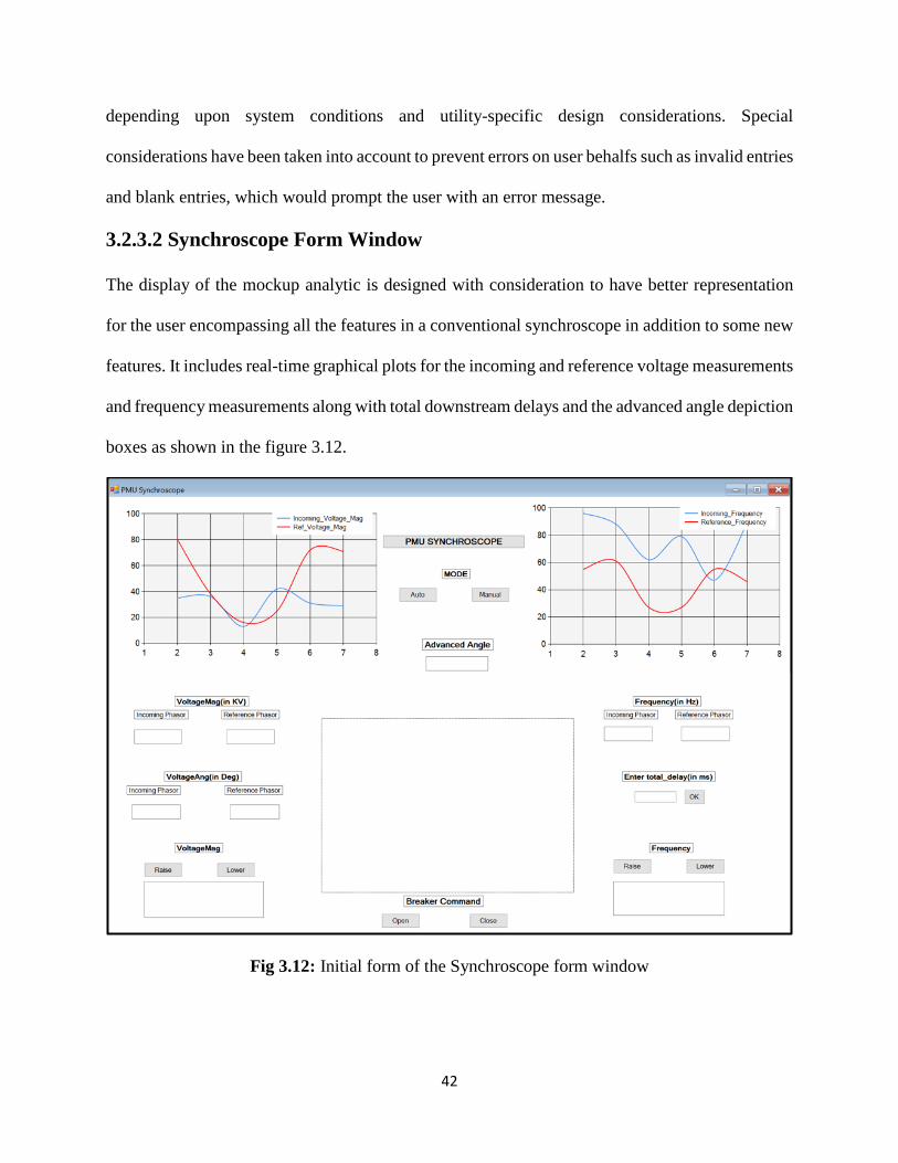
3.2.3.2 Synchroscope Form Window

The display of the mockup analytic is designed with consideration to have better representation

for the user encompassing all the features in a conventional synchroscope in addition to some new

features. It includes real-time graphical plots for the incoming and reference voltage measurements

and frequency measurements along with total downstream delays and the advanced angle depiction

boxes as shown in the figure 3.12.

Fig 3.12: Initial form of the Synchroscope form window

43

This synchroscope form is continuously updated invoking the “Update_measurements” method as

depicted below which outputs the breaker close or open command signal in each frame (which is

same as the frame rate of retrieval of PMU measurements from the openECA platform).

Fig 3.13: Code structure for Update_measurements method

The angular position of the rotating phasor hand inside the synchroscope form is updated based

upon the angular difference of the incoming voltage phase angle with respect to the reference

voltage phase angle which is subjected to the frame rate of retrieval of data from the openECA

platform (usually 30 frames per sec). However, the frame retrieval time can amount to a lower

value depending upon the system. To have a smooth transition between updating the synchroscope

form for a low retrieval frame rate case, a method named “TimeIntervalupdate” is invoked, which

retrieves the frequency slip in the current frame and would update the phasor hand to a predicted

value of angular difference position until the next frame is received. This prediction is made based

upon principle as described in equation (1) in chapter 2, under the assumption that no significant

changes would have occurred in the system until the next frame is received. If the frequency has

changed, then the actual position of the phasor hand based upon the new phase angle difference

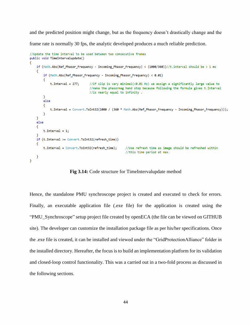
44

and the predicted position might change, but as the frequency doesn’t drastically change and the

frame rate is normally 30 fps, the analytic developed produces a much reliable prediction.

Fig 3.14: Code structure for TimeIntervalupdate method

Hence, the standalone PMU synchroscope project is created and executed to check for errors.

Finally, an executable application file (.exe file) for the application is created using the

“PMU_Synchroscope” setup project file created by openECA (the file can be viewed on GITHUB

site). The developer can customize the installation package file as per his/her specifications. Once

the .exe file is created, it can be installed and viewed under the “GridProtectionAlliance” folder in

the installed directory. Hereafter, the focus is to build an implementation platform for its validation

and closed-loop control functionality. This was a carried out in a two-fold process as discussed in

the following sections.

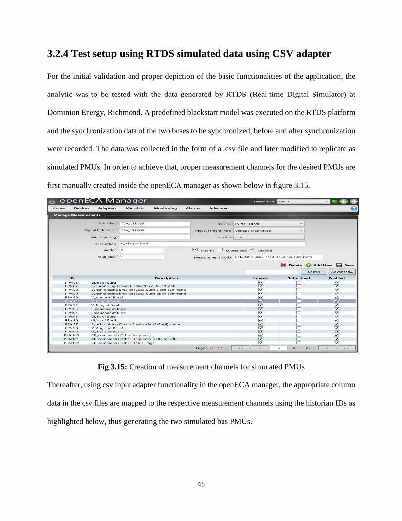
45

3.2.4 Test setup using RTDS simulated data using CSV adapter

For the initial validation and proper depiction of the basic functionalities of the application, the

analytic was to be tested with the data generated by RTDS (Real-time Digital Simulator) at

Dominion Energy, Richmond. A predefined blackstart model was executed on the RTDS platform

and the synchronization data of the two buses to be synchronized, before and after synchronization

were recorded. The data was collected in the form of a .csv file and later modified to replicate as

simulated PMUs. In order to achieve that, proper measurement channels for the desired PMUs are

first manually created inside the openECA manager as shown below in figure 3.15.

Fig 3.15: Creation of measurement channels for simulated PMUs

Thereafter, using csv input adapter functionality in the openECA manager, the appropriate column

data in the csv files are mapped to the respective measurement channels using the historian IDs as

highlighted below, thus generating the two simulated bus PMUs.

46

Fig 3.16: Using csv adapter to generate simulated PMUs

The observations after the execution of the RTDS simulated data are explained in detail in the next

chapter.

3.2.5 Test setup using OPAL-RT ePHASORSIM simulator

The RTDS simulated data was a test for validation and proper depiction of using openECA

platform with the developed analytic, but it did not encompass a closed loop control where the

user can initiate breaker command signals back to the openECA platform or any power system

model. To achieve this functionality, Dominion Energy procured an ePHASORSIM digital phasor

simulator manufactured by OPAL-RT technologies for the project. ePHASORSIM is a a tool for

projects that involve dynamic simulation of power systems and is used for the testing and

integration of EMS/SCADA systems, wide area protection, and control schemes, training and

power system studies and simulations in real time. ePHASORSIM’s phasor domain solver,

performing at a typical time-step of few milliseconds, provides voltage and current information

47

representing the same as phasor measurement unit (PMU) installed in the power grid [22]. This

unique electromechanical real-time simulation system enables precise simulation of large-scale

networks within a real-time and faster performance. ePHASORSIM real-time simulation is

performed under the OPAL-RT’s flagship RT-LAB simulation platform. It allows ePHASORSIM

to be connected as part of a larger Simulink model, enabling researchers to benefit from a complete

grid ecosystem, as well as having access to all OPAL-RT hardware modules and I/O and

communication protocols such as DNP3, OPC-UA, C37.118 and interconnect the real-time

simulation with physical devices under test [22]. The platform also offers all features for

monitoring, data processing and data acquisition to facilitate testing, analysis, and reporting. A

collection of models for the positive sequence as well as three-phase unbalanced power grids is

provided in a library of ePHASORSIM. The library includes models of generators and their

controllers, loads, transformers, current injector devices and voltage sources, along with various

types of events associated with each component to simulate complex operating and control

scenarios in real-time. For the synchroscope application, the inbuilt models provided by

ePHASORSIM have been used as a benchmark model with modifications.

The closed-loop feedback functionality of the PMU synchroscope can be demonstrated with the

help of the creation of a two islanded model system, and the measurements of the two buses to be

synchronized emulated as two separate PMU measurements. For demonstration purpose, real-time

simulated PMU data are streamed in using the OPAL-RT ePHASORSIM simulator. A custom

modified two islanded model for the 39 bus IEEE system is generated and executed on the target

simulator. The PMU Synchroscope is installed on the same desktop PC as openECA and

establishes a connection with openECA over GEP (Gateway Exchange Protocol) for input and

output measurements. Figure 3.17 depicts the information flow diagram of the test setup.

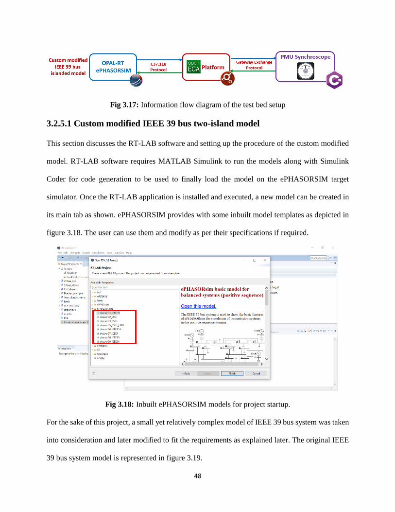
48

Fig 3.17: Information flow diagram of the test bed setup

3.2.5.1 Custom modified IEEE 39 bus two-island model

This section discusses the RT-LAB software and setting up the procedure of the custom modified

model. RT-LAB software requires MATLAB Simulink to run the models along with Simulink

Coder for code generation to be used to finally load the model on the ePHASORSIM target

simulator. Once the RT-LAB application is installed and executed, a new model can be created in

its main tab as shown. ePHASORSIM provides with some inbuilt model templates as depicted in

figure 3.18. The user can use them and modify as per their specifications if required.

Fig 3.18: Inbuilt ePHASORSIM models for project startup.

For the sake of this project, a small yet relatively complex model of IEEE 39 bus system was taken

into consideration and later modified to fit the requirements as explained later. The original IEEE

39 bus system model is represented in figure 3.19.

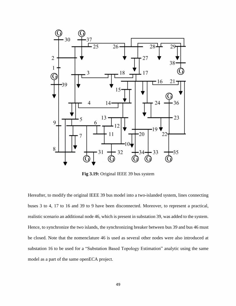
49

Fig 3.19: Original IEEE 39 bus system

Hereafter, to modify the original IEEE 39 bus model into a two-islanded system, lines connecting

buses 3 to 4, 17 to 16 and 39 to 9 have been disconnected. Moreover, to represent a practical,

realistic scenario an additional node 46, which is present in substation 39, was added to the system.

Hence, to synchronize the two islands, the synchronizing breaker between bus 39 and bus 46 must

be closed. Note that the nomenclature 46 is used as several other nodes were also introduced at

substation 16 to be used for a “Substation Based Topology Estimation” analytic using the same

model as a part of the same openECA project.

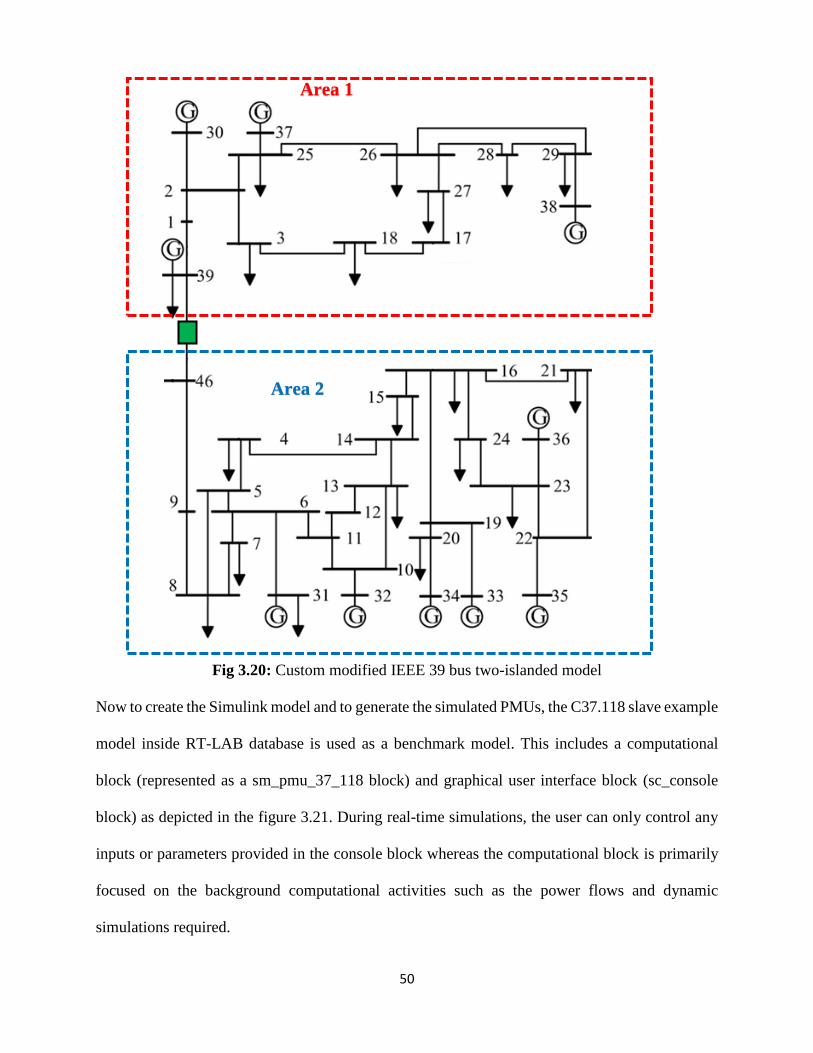
50

Fig 3.20: Custom modified IEEE 39 bus two-islanded model

Now to create the Simulink model and to generate the simulated PMUs, the C37.118 slave example

model inside RT-LAB database is used as a benchmark model. This includes a computational

block (represented as a sm_pmu_37_118 block) and graphical user interface block (sc_console

block) as depicted in the figure 3.21. During real-time simulations, the user can only control any

inputs or parameters provided in the console block whereas the computational block is primarily

focused on the background computational activities such as the power flows and dynamic

simulations required.

Area 1

Area 2

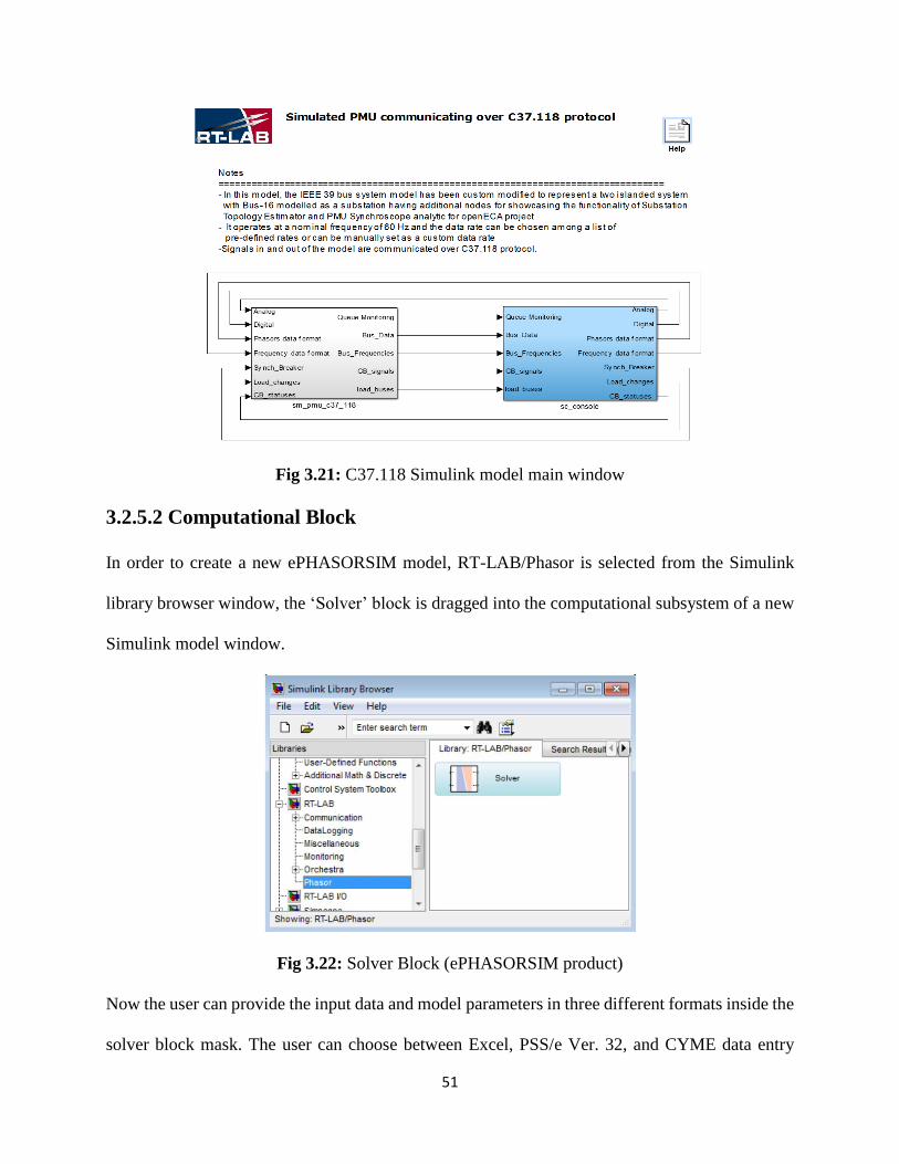
51

Fig 3.21: C37.118 Simulink model main window

3.2.5.2 Computational Block

In order to create a new ePHASORSIM model, RT-LAB/Phasor is selected from the Simulink

library browser window, the ‘Solver’ block is dragged into the computational subsystem of a new

Simulink model window.

Fig 3.22: Solver Block (ePHASORSIM product)

Now the user can provide the input data and model parameters in three different formats inside the

solver block mask. The user can choose between Excel, PSS/e Ver. 32, and CYME data entry

52

types. Each input format has distinct configurable parameters. The following figure shows the

‘Solver’ block mask configured for PSS/e input (Version 32).

Fig 3.23: Solver function Input file settings

If the PSS/e Ver. 32 input format is selected, only the ‘Pins’ page is required in the Excel input

file. Additionally, the following format-distinct items need to be configured, as follows.

The Pins file: It is an excel file which denotes the incoming and outgoing pins for the solver block.

There are two types of pins:

• Outgoing: To define measurement probes or monitor a status in the power system (e.g.

the voltage of a bus, or in-service status of a shunt device)

• Incoming: To send operational commands to the simulator (e.g. apply faults)

PSS/e RAW file: PSS/e's load flow data (*.raw).

PSS/e DYR file: PSS/e's dynamic data (*.dyr).

The simulation settings inside the solver mask, as depicted in the figure 3.24 are used to configure

the power-flow and dynamic simulation solvers.

53

Fig 3.24: Simulation settings inside the Solver block

These settings specify the behavior of the ‘Solver’ block when the simulation is executed. For the

purpose of the analytic, transients and dynamic behavior of the system after synchronization is

required to be monitored and hence, the “Power-flow and dynamic simulation” mode is selected.

In this particular execution mode, the solver block executes power-flow before running a dynamic

simulation. The solver initializes dynamic components based on voltage and power values

calculated by power-flow.

Now the Simulink model is created containing the solver block which contains the information for

the power system model and is configured to emulate PMUs to act as a C37.118 slave model which

can be loaded into the digital simulator as shown in figure 3.25.

54

Fig 3.25: Computational subsystem Simulink model architecture

Apart from acting in a C37.118 slave configuration, the model has to be configured as a C37.118

master configuration in order to receive the breaker commands back from the openECA platform.

This is achieved by incorporating the following two files along with the model.

1. The master driver configuration file (.config) which specifies the connection string for

the target simulator to receive the signals from the user system.

Fig 3.26: Master driver configuration file

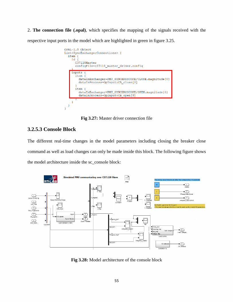
55

2. The connection file (.opal), which specifies the mapping of the signals received with the

respective input ports in the model which are highlighted in green in figure 3.25.

Fig 3.27: Master driver connection file

3.2.5.3 Console Block

The different real-time changes in the model parameters including closing the breaker close

command as well as load changes can only be made inside this block. The following figure shows

the model architecture inside the sc_console block:

Fig 3.28: Model architecture of the console block

56

The Synch Breaker Control block receives the command initiated from the application via

openECA platform and using the C37.118 master configuration driver of OPAL-RT as discussed

earlier. It finally relays the breaker status back into the solver block of the main computational

block as one of the incoming pins as seen in figure 3.25.

Fig 3.29: Synchronizing breaker control block

The highlighted region denotes the inclusion of delays in the system. It would represent both

communication delays and breaker closing delays (otherwise represented as the downstream

delays and termed constant as discussed earlier). Depending upon these delays, the breaker status

would be changed in the model after the signal from openECA is received, thus emulating practical

scenarios.

The load control block receives the frequency and voltage measurements, and the actual loads of

the load buses inside the island to be controlled as the inputs. As discussed earlier, depending upon

the slip in frequency and real-time voltage sensitivities calculations inside this block, the load

changes to be made are displayed. The operator can thereafter manually change the load as stated

in the algorithm specified earlier.

57

Fig 3.30: Load control block

3.2.5.4 Simulink Model configuration in RT-LAB

The Simulink model has been created, and the simulated PMU devices need to be created on the

RT-LAB main window under the configuration section of the model, which would be streaming

simulated PMU data over C37.118 protocol from the target simulator to the openECA platform.

Fig 3.31: Configuration of the simulated PMU devices

58

The various specifications for the streaming of data along with the data format are provided for

each simulated PMU device as shown in above figure. The next step is to connect the Simulink

model parameters with the virtual PMU devices that have been instantiated as depicted in figure

3.32.

Fig 3.32: Configuration of the phasors of the simulated PMU devices

As can be seen from figure 3.31, the different PMUs have been created, and the input and output

ports in the MATLAB Simulink model are mapped to the various measurements of any particular

PMU device. Once all this mapping is done, the Simulink model is loaded and finally executed on

the target simulator to stream real-time simulated data over C37.118 protocol.

3.2.6 Connection of the PMU devices to openECA platform

In this section, the procedure to retrieve the simulated stream of PMU data on the user system and

the openECA instance is discussed. For adding these, the configuration and connection files of the

respective PMU devices are required, which was collected using the “PMU Connection Tester”

open source application. Using these configuration and connection files, the various PMU devices

are then added to the openECA manager.

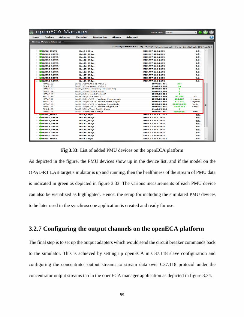
59

Fig 3.33: List of added PMU devices on the openECA platform

As depicted in the figure, the PMU devices show up in the device list, and if the model on the

OPAL-RT LAB target simulator is up and running, then the healthiness of the stream of PMU data

is indicated in green as depicted in figure 3.33. The various measurements of each PMU device

can also be visualized as highlighted. Hence, the setup for including the simulated PMU devices

to be later used in the synchroscope application is created and ready for use.

3.2.7 Configuring the output channels on the openECA platform

The final step is to set up the output adapters which would send the circuit breaker commands back

to the simulator. This is achieved by setting up openECA in C37.118 slave configuration and

configuring the concentrator output streams to stream data over C37.118 protocol under the

concentrator output streams tab in the openECA manager application as depicted in figure 3.34.

60

Fig 3.34: Configuring output streams for the breaker commands

Hence, a close loop feedback starting with the designing of the application followed by the

setting up of the simulator and its simulation settings to configuration of the simulated PMU

devices on the openECA instance and finally sending the breaker command signals from the

application via the openECA platform back to the simulator to modify the model parameters is

established. This particular setup helped us to demonstrate the comprehensive functionality of

the analytic in real time as discussed in the following chapter.

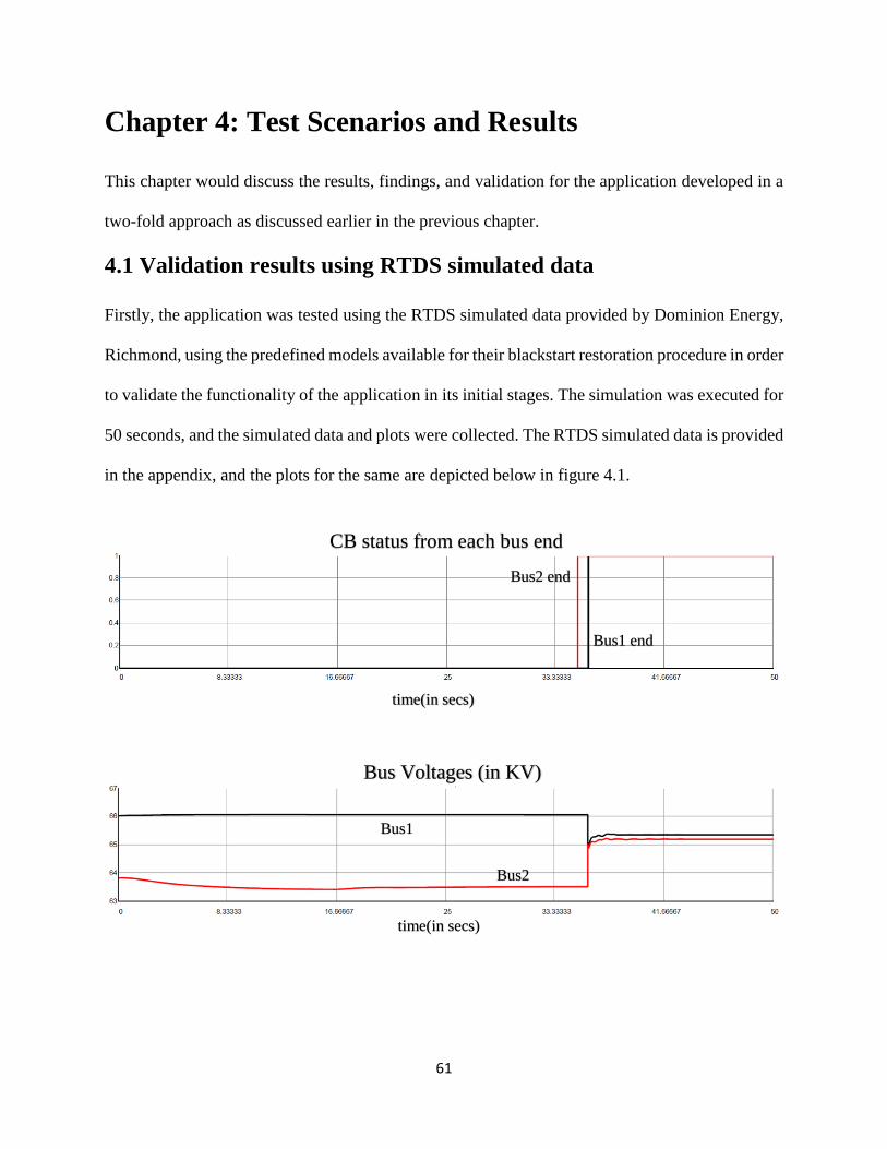
61

Chapter 4: Test Scenarios and Results

This chapter would discuss the results, findings, and validation for the application developed in a

two-fold approach as discussed earlier in the previous chapter.

4.1 Validation results using RTDS simulated data

Firstly, the application was tested using the RTDS simulated data provided by Dominion Energy,

Richmond, using the predefined models available for their blackstart restoration procedure in order

to validate the functionality of the application in its initial stages. The simulation was executed for

50 seconds, and the simulated data and plots were collected. The RTDS simulated data is provided

in the appendix, and the plots for the same are depicted below in figure 4.1.

CB status from each bus end

Bus Voltages (in KV)

Bus1 end

Bus2 end

time(in secs)

time(in secs)

Bus1

Bus2

62

Fig 4.1: RTDS simulated data plots prior and post-synchronization

As depicted in the above figure, the system conditions were modified to have the frequency of the

incoming island increase from below the reference frequency to finally surpass it. Thus, we have

a variable slip scenario setup but without any close loop control feedback. The movement of the

rotating phasor hand and the calculation of the advanced angle in order to correctly synchronize

finally at minimal (ideally zero) degree phase angle difference was found to be in accordance to

the data provided.

Bus Frequencies (in Hz)

Voltage phase angle difference (in rad)

time(in secs)

time(in secs)

Bus1

Bus2

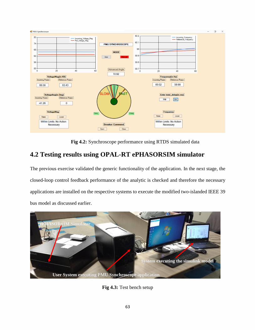
63

Fig 4.2: Synchroscope performance using RTDS simulated data

4.2 Testing results using OPAL-RT ePHASORSIM simulator

The previous exercise validated the generic functionality of the application. In the next stage, the

closed-loop control feedback performance of the analytic is checked and therefore the necessary

applications are installed on the respective systems to execute the modified two-islanded IEEE 39

bus model as discussed earlier.

Fig 4.3: Test bench setup

ePHASORSIM Simulator

User System executing PMU Synchroscope application

System executing the simulink model

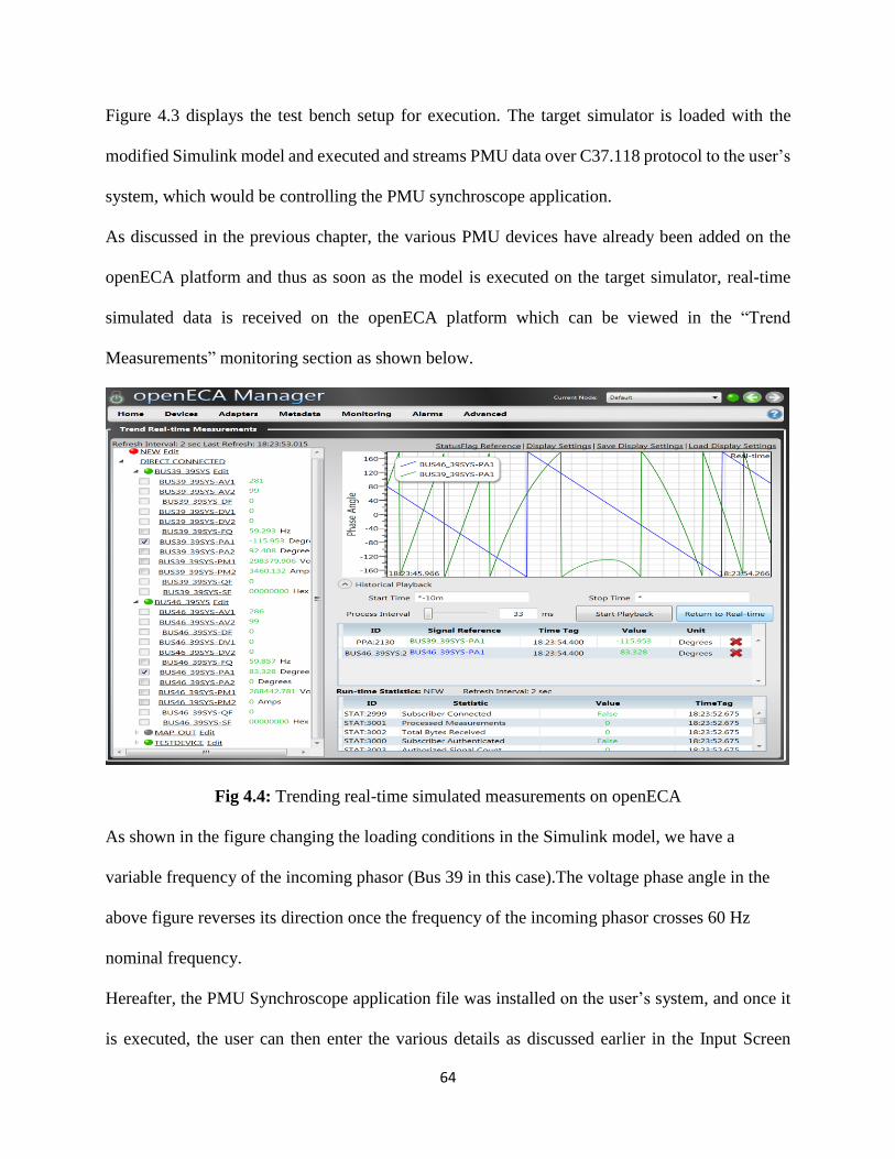
64

Figure 4.3 displays the test bench setup for execution. The target simulator is loaded with the

modified Simulink model and executed and streams PMU data over C37.118 protocol to the user’s

system, which would be controlling the PMU synchroscope application.

As discussed in the previous chapter, the various PMU devices have already been added on the

openECA platform and thus as soon as the model is executed on the target simulator, real-time

simulated data is received on the openECA platform which can be viewed in the “Trend

Measurements” monitoring section as shown below.

Fig 4.4: Trending real-time simulated measurements on openECA

As shown in the figure changing the loading conditions in the Simulink model, we have a

variable frequency of the incoming phasor (Bus 39 in this case).The voltage phase angle in the

above figure reverses its direction once the frequency of the incoming phasor crosses 60 Hz

nominal frequency.

Hereafter, the PMU Synchroscope application file was installed on the user’s system, and once it

is executed, the user can then enter the various details as discussed earlier in the Input Screen

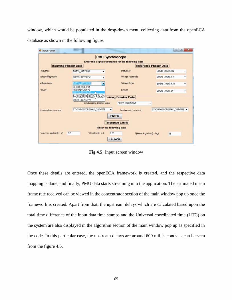
65

window, which would be populated in the drop-down menu collecting data from the openECA

database as shown in the following figure.

Fig 4.5: Input screen window

Once these details are entered, the openECA framework is created, and the respective data

mapping is done, and finally, PMU data starts streaming into the application. The estimated mean

frame rate received can be viewed in the concentrator section of the main window pop up once the

framework is created. Apart from that, the upstream delays which are calculated based upon the

total time difference of the input data time stamps and the Universal coordinated time (UTC) on

the system are also displayed in the algorithm section of the main window pop up as specified in

the code. In this particular case, the upstream delays are around 600 milliseconds as can be seen

from the figure 4.6.

66

Fig 4.6: Analytic Main Window

Hereafter, the tolerance limits for successful synchronization which can be user/utility specific

depending upon system conditions are provided, and the PMU synchroscope form window is

finally launched as shown in the figure below.

Fig 4.7: Synchroscope Form Window prior synchronization

67

A total downstream delay of 500 milliseconds is entered in this window and depending upon the

slip in frequency between the two buses, an advanced angle is calculated and displayed as shown

in the figure. The center of the synchroscope form depicts the breaker status, which is green in the

above figure denoting that the synchronizing breaker between Bus-39 and Bus-46 is open. As we

can see as the difference in the various measurements are out of the tolerance limits, proper

annunciations and respective actions are displayed highlighted in the blue boxes, and therefore,

the checklist indicates that the breaker close command cannot be initiated. Once respective actions

are carried out by the operator and the measurements across both sides of the synchronizing

breaker are brought within respective tolerance limits, the breaker close command can either be

initiated manually in “Manual” mode or automatically sensed by the application at the advanced

angle position in the “Auto” mode.

Fig 4.8: Synchroscope Form Window post synchronization

68

It can be observed from figure 4.8, that the transients after the synchronization are acceptable and

dies out after some interval, thus leading to proper and successful synchronization.

As discussed earlier, the synchroscope application would only raise annunciations communicating

to the user how much change in the measurements needs to be achieved. But it doesn’t direct the

procedure how to achieve it and thus, the following section discusses the performance of the load

control technique using voltage sensitivities of the load buses of only one island which is to be

controlled (in this case the incoming island which is Area -1) as discussed in the earlier chapters .

This technique also helps to reduce the after synchronization transients as the slip between the two

islands is reduced to a minimal value. Two scenarios are considered to depict the load control

technique functionality and how the operator might utilize this for controlling the frequency of the

island.

1. The incoming phasor frequency is higher than the reference phasor frequency.

2. The incoming phasor frequency is lower than the reference phasor frequency.

Scenario-1:

In both the scenarios, the loading in area-2 (Reference island) is modified to maintain a reference

phasor frequency of 60.01 Hz. Now modifying the system conditions and maintaining the loading

conditions as depicted below in the table, the frequency of Area-1 is brought to 60.19 Hz. The

following table depicts the loads at the various PQ buses in Area-1.

Bus Number Load (in MW)

3 356.6

18 172

25 217

26 140

69

27 296

28 206

29 282

39 919.355

Table 4.1: Loads at various PQ buses of Area-1 prior load control (Scenario-1)

The voltage phase angle profile of the two islands with such a large slip can be visualized from the

following figure.

Fig 4.9: Voltage phase angle profile prior load control (Scenario-1)

Now the loading conditions have to be modified in order to bring the frequency of the incoming

phasor as close to the reference phasor. As in this scenario, the incoming frequency is greater than

the reference frequency, the total load to be shed for achieving a frequency close to the reference

phasor can be calculated using the equation (14). For calculating this value, the equivalent inertia

constant of the multi-machine system (Area-1) has to be calculated first.

Area-1

Area-2

70

The inertia constants of the four generators inside Area 1 are noted in the following table.

Generator Bus number Inertia constant H (in secs)

30 4.2

37 2.43

38 3.45

39 50

Table 4.2: Inertia constants of the various generators in Area-1

The equivalent Heq of Area-1 amounts to

𝐻𝑒𝑞 = ∑ 𝐻𝑖𝑛𝑖=1 =4.2+2.43+3.45+50=60.08 (20)

For testing for this project, the settling time after the overall load change was scheduled to take

effect within 5 seconds. Thus plugging in the values in equation 14, the total Pdiff or total load

change was calculated to be

𝑃𝑑𝑖𝑓𝑓𝑒𝑞 =2𝐻𝑒𝑞

𝑓0(

𝑓𝑖𝑛𝑐𝑜𝑚𝑖𝑛𝑔 − 𝑓𝑟𝑒𝑓𝑒𝑟𝑒𝑛𝑐𝑒

𝑡𝑑𝑖𝑓𝑓) =

2 ∗ 60.08

60∗ (

60.19 − 60.01

5)

⇒ 𝑃𝑑𝑖𝑓𝑓𝑒𝑞 = 0.072096 𝑝. 𝑢. = 72.096 𝑀𝑊 (21)

Note: The Base MVA is taken as 1000 MVA

Hence, the total amount of load to be shed throughout the island is around 72 MW.

Secondly, the order of load shed at the different PQ buses can be decided by the operator either

based upon the voltage magnitudes in ascending order or the load availability upon analysis. Next,

executing the algorithm for calculating the share at each load bus based upon voltage sensitivity

analysis as per equation (18) in the Simulink model, the technique directs the operator to change

the loading to following conditions.

71

Bus Number Load (in MW)

3 363.2

18 176.7

25 223.4

26 147

27 303.4

28 216.8

29 288.4

39 942.3

Table 4.3: Loads at various PQ buses of Area-1 post load control (Scenario-1)

The operator can use these values to change the loading in the order earlier discussed based upon

different bus voltage profiles. Once this is achieved, the frequency of the incoming island reduces

down to 60.02 Hz (very much closer to the reference frequency). The voltage phase angle profile

of the two islands has been modified as follows.

Fig 4.10: Voltage phase angle profile post load control (Scenario-1)

Area-1

Area-2

72

The operator can now close the synchronizing breakers if all other conditions for voltage

magnitude and angles are within limits and would thus lead to minimal after synchronization

transients and much smoother synchronization.

Scenario-2:

Now modifying the system conditions and maintaining the loading conditions as depicted below

in the table, a frequency of 59.83 Hz for Area-1 (incoming island) is achieved. The following table

depicts the loads at the various PQ buses in Area-1 prior load control.

Bus Number Load (in MW)

3 363.2

18 176.7

25 223.4

26 147

27 303.4

28 216.8

29 288.4

39 1025.346

Table 4.4: Loads at various PQ buses of Area-1 prior load control (Scenario-2)

The voltage phase angle profile of the two islands with the incoming phasor frequency lesser

than the reference phasor frequency is depicted in the following figure.

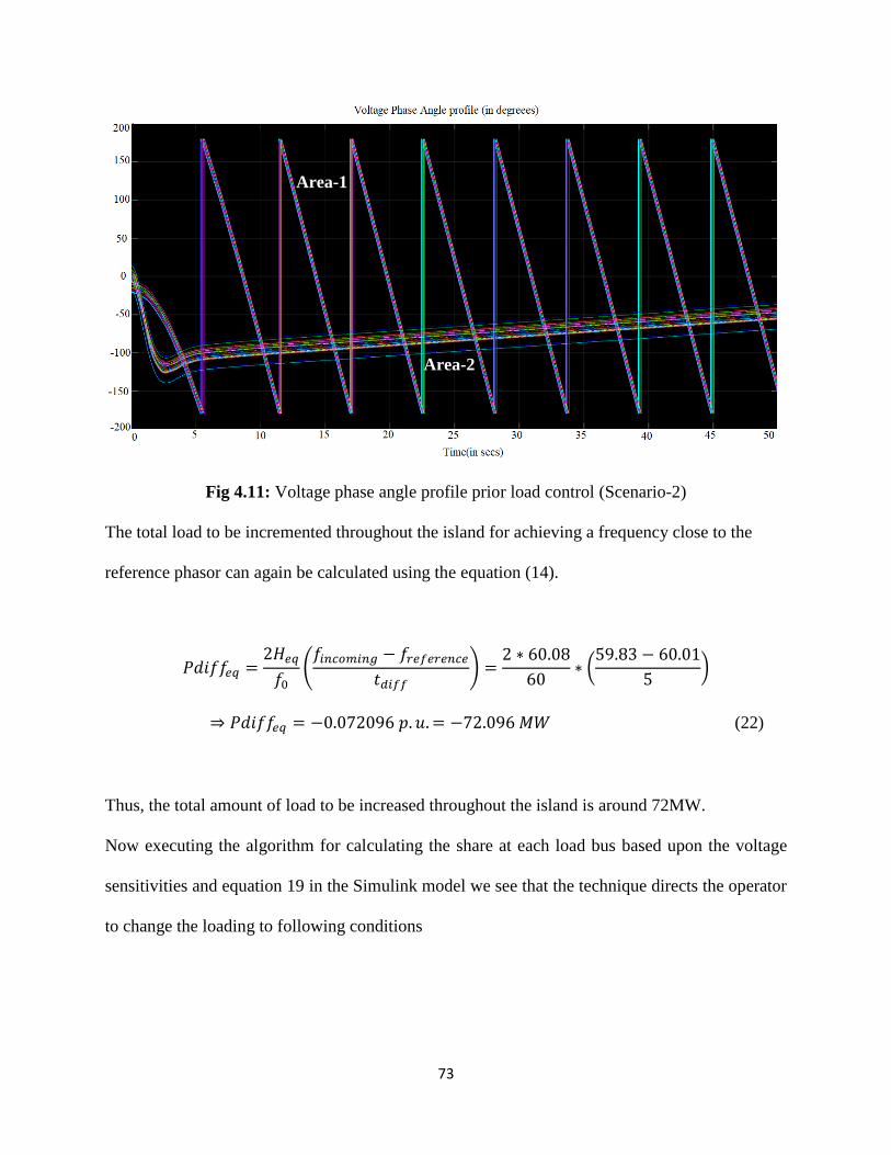
73

Fig 4.11: Voltage phase angle profile prior load control (Scenario-2)

The total load to be incremented throughout the island for achieving a frequency close to the

reference phasor can again be calculated using the equation (14).

𝑃𝑑𝑖𝑓𝑓𝑒𝑞 =2𝐻𝑒𝑞

𝑓0(

𝑓𝑖𝑛𝑐𝑜𝑚𝑖𝑛𝑔 − 𝑓𝑟𝑒𝑓𝑒𝑟𝑒𝑛𝑐𝑒

𝑡𝑑𝑖𝑓𝑓) =

2 ∗ 60.08

60∗ (

59.83 − 60.01

5)

⇒ 𝑃𝑑𝑖𝑓𝑓𝑒𝑞 = −0.072096 𝑝. 𝑢. = −72.096 𝑀𝑊 (22)

Thus, the total amount of load to be increased throughout the island is around 72MW.

Now executing the algorithm for calculating the share at each load bus based upon the voltage

sensitivities and equation 19 in the Simulink model we see that the technique directs the operator

to change the loading to following conditions

Area-1

Area-2

74

Bus Number Load (in MW)

3 355.7

18 171.7

25 216

26 139

27 295

28 204.4

29 281

39 998.8

Table 4.5: Loads at various PQ buses of Area-1 post load control (Scenario-2)

Once the loading is changed as per these requirements, the frequency of the incoming island rises

to 60.00 Hz (very much closer to the reference frequency). The voltage phase angle profile of the

two islands has been modified as follows.

Fig 4.12: Voltage phase angle profile post load control (Scenario-2)

Area-1

Area-2

75

The technique was found to be quite effective in regulating the frequency of the incoming island

as desired. The most important thing to consider such a technique is because of a blackstart

scenario during which the utilities have ample control of changing or modifying the loads across

different areas which might not be feasible during normal scenarios. However, the purpose of

inclusion of such a technique is to show how any control technique can be incorporated into the

synchroscope and can be tailor-made for specific utilities as required.

The after synchronization transients were minimal and led to smoother and successful

synchronization in both the cases.

Fig 4.13: Smoother synchronization with inclusion of load control

76

Chapter-5: Conclusion and Future Work

5.1 Conclusion

This thesis document discusses the implementation of a synchrophasor based centralized remote

synchroscope (otherwise referred to as PMU synchroscope in the document) as a part of the

development of analytics for the DOE-sponsored openECA project. The basic idea to achieve such

functionality at a remote central location (such as the utility’s control room) was to overcome the

various delays associated in a wide area measurement system, which would have eventually

hindered the accurate time synchronized breaker closing action at the substation. The concept of

advanced angle was used and a modified synchroscope application supporting all features of the

traditional physical synchroscope with the inclusion of some additional features was created which

can be used for immediate implementation if required in the utility sector compatible to the

openECA platform. The synchroscope restricts the chances of errors made on behalf of the

user/operator and raises appropriate annunciations/alarms to notify how much of a change is

required for the measurements of the two buses to be synchronized. In order to demonstrate how

to achieve these modifications (which ultimately would be user/utility specific procedures), a load

control technique based on the algorithm stated in [21] is used with minor modifications.

Satisfactory results were obtained with the inclusion of such an algorithm. The after

synchronization transients were minimized and hence, leading to much smoother and successful

synchronization. However, the important point to note is that this type of technique would be more

feasible for the utility during blackstart or bulk power system restoration as they would have much

more flexibility on loads during this time as compared to normal situations.

77

5.2 Future work

The openECA application along with most of the analytics associated with it are a part of the open

source project. The PMU synchroscope developed was built in C# language and has been uploaded

to the GITHUB site, and the web links are provided in the appendix. This provides a great

opportunity for power system researchers or utility personnel to look on the web and can start

modifying the application to tailor fit as per their requirements. The most crucial modification that

can be added to this project is the inclusion of real-time downstream delays for the channel to be

used to send back the breaker commands in the GUI of the synchroscope. This would further

reduce error on behalf of the user and would lead to much smoother and more successful time

synchronization between the two buses. Apart from that, as voltage control and frequency control

were beyond the scope of this project, possible future work might be the inclusion of these aspects

within the PMU synchroscope application, which might be custom made individual utility

differently, depending upon their system parameters and system topology. In this way, a more

comprehensive delay incorporated PMU synchroscope for the ease of the user/operator can be

built.

78

References

[1] R. J. Campbell, “Weather-Related Power Outages and Electric System Resiliency,”

Washington DC, USA: Library of Congress, 2012.

[2] S. H. Conrad, R. J. LeClaire, G. P. O’Reilly and H. Uzunalioglu, “Critical national

infrastructure reliability modeling and analysis,” Bell Labs Tech. J., vol. 11, no. 3, pp. 57–71,

2006.

[3] E. Mills. “Electric grid disruptions and extreme weather.” [Online]. Available:

http://evanmills.lbl.gov/presentations/Mills-Grid- Disruptions-NCDC-3May2012.pdf

[4] M. M. Adibi and L. H. Fink, “Overcoming restoration challenges associated with major

power system disturbances—Restoration from cascading failures,” IEEE Power Energy Mag., vol.

4, no. 5, pp. 68–77, Sep. 2006.

[5] M. M. Adibi and L. H. Fink, “Power system restoration planning,” IEEE Trans. Power Syst.,

vol. 9, no. 1, pp. 22–28, Feb. 1994.

[6] Feng Qiu, Peijie Li, “An Integrated Approach for Power System Restoration Planning,”

Proceedings of the IEEE, 2017.

[7] Qin Zhijun, Liu Shanshan, Hou Yunhe, “Virtual Synchroscope: a novel application of PMU

for system restoration,” 2011The International Conference on Advanced Power System

Automation and Protection.

[8] S. Kolluri, S. Mandal, F. Galvan, and M. Thomas, “Island formation in Entergy power grid

during Hurricane Gustav” in Power & Energy Society General Meeting, 2009. PES '09. IEEE,

2009, pp. 1-5.

[9] S. Corsi and C. Sabelli, “General blackout in Italy Sunday September 28, 2003, h. 03:28:00”

in Power Engineering Society General Meeting, 2004,IEEE, 2004, pp. 1691-1702 Vol.2.

79

[10] “Final Report of the Investigation Committee on the 28 September 2003 Blackout in Italy,”

UCTE Report – April 2004.

[11] Konstantinos Diakos, Qiuwei Wu, Arne Hejde Nielsen, “Phasor Measurement Unit and

Phasor Data Concentrator test with Real-Time Digital Simulator,” 2014 IEEE PES Asia-Pacific

Power and Energy Engineering Conference (APPEEC)

[12] IEEE Guide for Phasor Data Concentrator Requirements for Power System Protection,

Control, and Monitoring.

[13] Richard C Schaefer, “Art of Generator Synchronizing,” IEEE Transactions on Industry

Applications, 2017.

[14] Michael J. Thompson, “Fundamentals and Advancements in Generator Synchronizing

Systems,” 2012 65th Annual Conference for Protective Relay Engineers.

[15] Daniel L. Ransom, “Get in Step with Synchronization,” 2014 IEEE/IAS 50th Industrial &

Commercial Power Systems Technical Conference.

[16] C. W. Taylor, V. Venkatasubramanian, and Y. Chen, “Wide-area stability and voltage

control,” in Proc. 2002, 7th Symp. Specialists in Electric Operational and Expansion Planning, pp.

1–9.

[17] F. Zhang, Y. Sun, L. Cheng, X. Li, J.H. Chow, and W. Zhao, “Measurement and Modeling of

Delays in Wide-Area Closed-Loop Control Systems,”, 2015 IEEE Transactions on Power Systems

[18] W. Liu, H. Luo, S. Li, and D. Gao, “Investigation and modeling of communication delays in

wide area measurement system,” in Proc. 2012 Asia-Pacific, Power and Energy Eng. Co

[19] Z. Hu, X. Xie, J. Xiao, and L. Tong, “Analysis and test on delays in the wide area measuring

system,” Autom. Elect. Power Syst., vol. 28, no. 15, pp. 39–43, 2004.nf. (APPEEC), pp. 1–4.

80

[20] Prithwish Mukhopadhyay, Pushpa Seshadri, Chitranshi Gangrekar, Chandan Kumar, Awani

Bhusan Rai, Naveen M. Reddy, “WAMS and Synchrophasor experience during synchronization

of Large grids in India,” 2015 IEEE International Conference on Signal Processing, Informatics,

Communication, and Energy Systems (SPICES).

[21] Poonam Joshi, “Load Shedding Algorithm Using Voltage and Frequency Data,” Master’s

Thesis, Clemson University, 2007.

[22] https://www.opal-rt.com/systems-ephasorsim

[23] M. Parniani, A. Nasri, “SCADA based under frequency load shedding integrated with rate of

frequency decline,” 2006 IEEE Power Engineering Society General Meeting.

[24] D Yang, Z Nie, K Jones, V Centeno, “Adaptive decision-trees-based regional voltage

control,” 2017 North American Power Symposium (NAPS).

[25] Duotong Yang, Dissertation on “A Data Analytics Framework for Regional Voltage Control,”

2017 Virginia Tech.

[26] Hung-Ming Chou, Chetan Mishra, Yajun Wang & Michael K. Thomas, “Application of

RTDS as Real-Time Decision Support Tool,” Grid of the Future Symposium, 2017 CIGRE.

[27] Anamitra Pal, Chetan Mishra, Anil Kumar S Vullikanti & SS Ravi, “General optimal

substation coverage algorithm for phasor measurement unit placement in practical systems,” 2017

IET Generation, Transmission & Distribution, 11, 347-353.

[28] Dao Zhou, Jiahui Guo, Ye Zhang, Jidong Chai, Hesen Liu, Yong Liu, Can Huang, Xun Gui,

Yilu Liu. “Distributed Data Analytics Platform for Wide-Area Synchrophasor Measurement

Systems”, IEEE Trans. Smart Grid, 2016, 2397- 2405.

81

Appendix

Related Links

[1] https://github.com/GridProtectionAlliance/openECA

[2] http://www.opal-rt.com/systems-ephasorsim

[3] https://github.com/tapasbarik/Analytics/blob/master/PMU_Synchroscope_Final.zip