Synchrosqueezed wavelet transforms: An empirical mode ... · function, or the wavelet transform, where the templates are obtained by translating and dilating the basic (or “mother”)

Appl. Comput. Harmon. Anal. 30 (2011) 243–261

Contents lists available at ScienceDirect

Applied and Computational Harmonic Analysis

www.elsevier.com/locate/acha

Synchrosqueezed wavelet transforms: An empirical modedecomposition-like tool

Ingrid Daubechies, Jianfeng Lu ∗,1, Hau-Tieng Wu

Department of Mathematics and Program in Applied and Computational Mathematics, Princeton University, Princeton, NJ 08544, United States

a r t i c l e i n f o a b s t r a c t

Article history:Received 12 December 2009Revised 11 August 2010Accepted 13 August 2010Available online 20 August 2010Communicated by Patrick Flandrin

Keywords:WaveletTime-frequency analysisSynchrosqueezingEmpirical mode decomposition

The EMD algorithm is a technique that aims to decompose into their building blocksfunctions that are the superposition of a (reasonably) small number of components, wellseparated in the time–frequency plane, each of which can be viewed as approximatelyharmonic locally, with slowly varying amplitudes and frequencies. The EMD has alreadyshown its usefulness in a wide range of applications including meteorology, structuralstability analysis, medical studies. On the other hand, the EMD algorithm contains heuristicand ad hoc elements that make it hard to analyze mathematically.In this paper we describe a method that captures the flavor and philosophy of theEMD approach, albeit using a different approach in constructing the components. Theproposed method is a combination of wavelet analysis and reallocation method. Weintroduce a precise mathematical definition for a class of functions that can be viewedas a superposition of a reasonably small number of approximately harmonic components,and we prove that our method does indeed succeed in decomposing arbitrary functions inthis class. We provide several examples, for simulated as well as real data.

© 2010 Elsevier Inc. All rights reserved.

1. Introduction

Time-frequency representations provide a powerful tool for the analysis of time series signals. They can give insight intothe complex structure of a “multi-layered” signal consisting of several components, such as the different phonemes in aspeech utterance, or a sonar signal and its delayed echo. There exist many types of time-frequency (TF) analysis algorithms;the overwhelming majority belong to either “linear” or “quadratic” methods [1].

In “linear” methods, the signal to be analyzed is characterized by its inner products with (or correlations with) apre-assigned family of templates, generated from one (or a few) basic template by simple operations. Examples are thewindowed Fourier transform, where the family of templates is generated by translating and modulating a basic windowfunction, or the wavelet transform, where the templates are obtained by translating and dilating the basic (or “mother”)wavelet. Many linear methods, including the windowed Fourier transform and the wavelet transform, make it possible toreconstruct the signal from the inner products with templates; this reconstruction can be for the whole signal, or for partsof the signal; in the latter case, one typically restricts the reconstruction procedure to a subset of the TF plane. However,in all these methods, the family of template functions used in the method unavoidably “colors” the representation, and caninfluence the interpretation given on “reading” the TF representation in order to deduce properties of the signal. Moreover,the Heisenberg uncertainty principle limits the resolution that can be attained in the TF plane; different trade-offs can beachieved by the choice of the linear transform or the generator(s) for the family of templates, but none is ideal, as illustrated

* Corresponding author.E-mail addresses: [email protected] (I. Daubechies), [email protected] (J. Lu), [email protected] (H.-T. Wu).

1 Current address: Courant Institute of Mathematical Sciences, New York University, New York, NY 10012, United States.

1063-5203/$ – see front matter © 2010 Elsevier Inc. All rights reserved.doi:10.1016/j.acha.2010.08.002

http://dx.doi.org/10.1016/j.acha.2010.08.002

http://www.ScienceDirect.com/

http://www.elsevier.com/locate/acha

mailto:[email protected]



http://dx.doi.org/10.1016/j.acha.2010.08.002

244 I. Daubechies et al. / Appl. Comput. Harmon. Anal. 30 (2011) 243–261

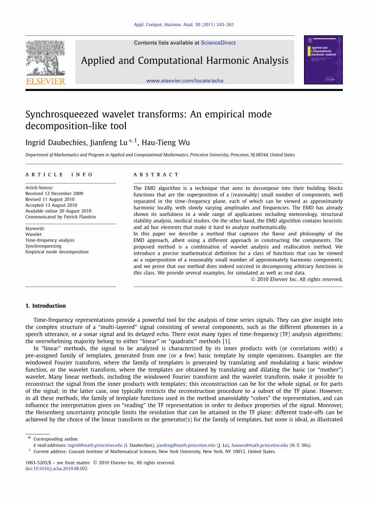
Fig. 1. Examples of linear time-frequency representations. Top row: the signal s(t) = s1(t) + s2(t) (top left) defined by s1(t) = 0.5t + cos(20t) for 0 � t �5π/2 (top middle) and s2(t) = cos( 4

3 [(t − 10)3 − (2π − 10)3] + 10(t − 2π)) for 2π � t � 4π (top right). Next row: left: the instantaneous frequencyfor its two components (left) ω(t) = 20 for 0 � (t − 10)2 � 5π/2, and ω(t) = 4t2 + 10 for 2π � t � 4π ; middle: two examples of (the absolute valueof) a continuous windowed Fourier transform of s(t), with a wide window (2π/5) (top) and a narrow window (π/10) (bottom) [these are plotted withMatlab, with the ‘jet’ colormap; red indicates higher amplitude]; right: two examples of a continuous wavelet transform of s(t), with a Morlet wavelet (top)and a Haar wavelet (bottom) [plotted with ‘hsv’ colormap in Matlab; purple indicates higher amplitude]. The instantaneous frequency profile can be clearlyrecognized in each of these linear TF representations, but it is “blurred” in each case, in different ways that depend on the choice of the transform. (Forinterpretation of colors in this figure, the reader is referred to the web version of this article.)

Fig. 2. Examples of quadratic time-frequency representations. Left: the Wigner–Ville transform of s(t), in which interference causes the typical Moirépatterns; middle and right: two pseudo-Wigner–Ville transforms of s(t), obtained by blurring the Wigner–Ville transform slightly using Gaussian smoothing(middle) and somewhat more (right). [All three graphs plotted with ‘jet’ colormap in Matlab, calibrated identically.] The blurring removes the interferencepatterns, at the cost of precise location in the time-frequency localization.

in Fig. 1. In “quadratic” methods to build a TF representation, one can avoid introducing a family of templates with whichthe signal is “compared” or “measured”. As a result, some features can have a crisper, “more focused” representation in theTF plane with quadratic methods (see Fig. 2). However, in this case, “reading” the TF representation of a multi-componentsignal is rendered more complicated by the presence of interference terms between the TF representations of the individualcomponents; these interference effects also cause the “time-frequency density” to be negative in some parts of the TF plane.These negative parts can be removed by some further processing of the representation [1], at the cost of reintroducing someblur in the TF plane. Reconstruction of the signal, or part of the signal, is much less straightforward for quadratic than forlinear TF representations.

In many practical applications, in a wide range of fields (including, e.g., medicine and engineering) one is faced withsignals that have several components, all reasonably well localized in TF space, at different locations. The components

I. Daubechies et al. / Appl. Comput. Harmon. Anal. 30 (2011) 243–261 245

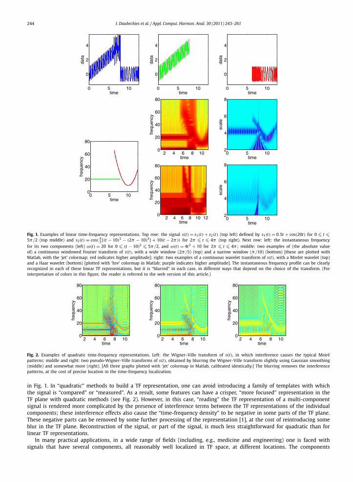
Fig. 3. Two examples of wave functions of the type cos[φ(t)], with slowly varying A(t) and φ′(t), for which standard TF representations are not very welllocalized in the time–frequency plane. Left: signal; middle left: windowed Fourier transform; middle right: Morlet wavelet transform; right: Wigner–Villefunction. [All TF representations plotted with ‘jet’ colormap in Matlab.]

are often also called “non-stationary”, in the sense that they can present jumps or changes in behavior, which it may beimportant to capture as accurately as possible. For such signals both the linear and quadratic methods come up short.Quadratic methods obscure the TF representation with interference terms; even if these could be dealt with, reconstructionof the individual components would still be an additional problem. Linear methods are too rigid, or provide too blurred apicture. Figs. 1, 2 show the artifacts that can arise in linear or quadratic TF representations when one of the componentssuddenly stops or starts. Fig. 3 shows examples of components that are non-harmonic, but otherwise perfectly reasonableas candidates for a single-component-signal, yet not well represented by standard TF methods, as illustrated by the lack ofconcentration in the time–frequency plane of the transforms of these signals. The Empirical Mode Decomposition (EMD)method was proposed by Norden Huang [2] as an algorithm that would allow time-frequency analysis of such multi-component signals, without the weaknesses sketched above, overcoming in particular artificial spectrum spread causedby sudden changes. Given a signal s(t), the method decomposes it into several intrinsic mode functions (IMF):

s(t) =K∑

k=1

sk(t), (1.1)

where each IMF is basically a function oscillating around 0, albeit not necessarily with constant frequency:

sk(t) = Ak(t) cos(φk(t)

), with Ak(t),φ

′k(t) > 0 ∀t. (1.2)

(Here, and throughout the paper, we use “prime” to denote the derivative, i.e. g′(t) = dgdt (t).) Essentially, each IMF is an

amplitude modulated–frequency modulated (AM–FM) signal; typically, the change in time of Ak(t) and φ′k(t) is much slower

than the change of φk(t) itself, which means that locally (i.e. in a time interval [t − δ, t + δ], with δ ≈ 2π [φ′k(t)]−1) the

component sk(t) can be regarded as a harmonic signal with amplitude Ak(t) and frequency φ′k(t). (Note that this differs

from the definition given by Huang; in e.g. [2], the conditions on an IMF are phrased as follows: (1) in the whole data set,the number of extrema and the number of zero crossings of sk(t) must either be equal or differ at most by one; and (2) atany t , the value of a smooth envelope defined by the local minima of the IMF is the negative of the corresponding envelopedefined by the local maxima. Functions satisfying (1.2) have these properties, but the reverse inclusion doesn’t hold. Inpractice, the examples given in [2] and elsewhere typically do satisfy (1.2), however.) After the decomposition of s(t) intoits IMF components, the EMD algorithm proceeds to the computation of the “instantaneous frequency” of each component.Theoretically, this is given by ωk(t) := φ′

k(t); in practice, rather than a (very unstable) differentiation of the estimated φk(t),the originally proposed EMD method used the Hilbert transform of the sk(t) [2]; more recently, this has been replaced byother methods [3].

It is clear that the classes of functions that can be written in the form (1.1) with each component as in (1.2) is quitelarge. In particular, if s(t) is defined (or observed) in [−T , T ] with finite number terms in the Fourier series, then the Fourierseries on [−T , T ] of s(t) is such a decomposition. It is also easy to see that such a decomposition is far from unique. Thisis simply illustrated by considering the following signal:


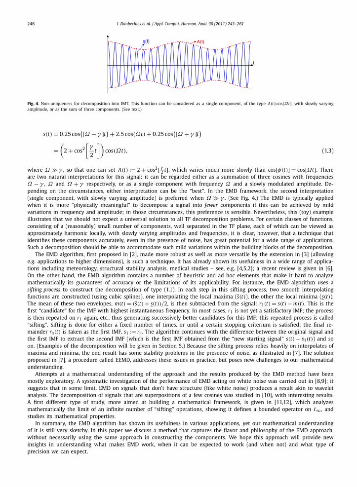
Fig. 4. Non-uniqueness for decomposition into IMT. This function can be considered as a single component, of the type A(t) cos[Ωt], with slowly varyingamplitude, or as the sum of three components. (See text.)

s(t) = 0.25 cos([Ω − γ ]t) + 2.5 cos(Ωt) + 0.25 cos

([Ω + γ ]t)=

(2 + cos2

[γ

2t

])cos(Ωt), (1.3)

where Ω � γ , so that one can set A(t) := 2 + cos2[ γ2 t], which varies much more slowly than cos[φ(t)] = cos[Ωt]. There

are two natural interpretations for this signal: it can be regarded either as a summation of three cosines with frequenciesΩ − γ , Ω and Ω + γ respectively, or as a single component with frequency Ω and a slowly modulated amplitude. De-pending on the circumstances, either interpretation can be the “best”. In the EMD framework, the second interpretation(single component, with slowly varying amplitude) is preferred when Ω � γ . (See Fig. 4.) The EMD is typically appliedwhen it is more “physically meaningful” to decompose a signal into fewer components if this can be achieved by mildvariations in frequency and amplitude; in those circumstances, this preference is sensible. Nevertheless, this (toy) exampleillustrates that we should not expect a universal solution to all TF decomposition problems. For certain classes of functions,consisting of a (reasonably) small number of components, well separated in the TF plane, each of which can be viewed asapproximately harmonic locally, with slowly varying amplitudes and frequencies, it is clear, however, that a technique thatidentifies these components accurately, even in the presence of noise, has great potential for a wide range of applications.Such a decomposition should be able to accommodate such mild variations within the building blocks of the decomposition.

The EMD algorithm, first proposed in [2], made more robust as well as more versatile by the extension in [3] (allowinge.g. applications to higher dimensions), is such a technique. It has already shown its usefulness in a wide range of applica-tions including meteorology, structural stability analysis, medical studies – see, e.g. [4,5,2]; a recent review is given in [6].On the other hand, the EMD algorithm contains a number of heuristic and ad hoc elements that make it hard to analyzemathematically its guarantees of accuracy or the limitations of its applicability. For instance, the EMD algorithm uses asifting process to construct the decomposition of type (1.1). In each step in this sifting process, two smooth interpolatingfunctions are constructed (using cubic splines), one interpolating the local maxima (s(t)), the other the local minima (s(t)).The mean of these two envelopes, m(t) = (s(t) + s(t))/2, is then subtracted from the signal: r1(t) = s(t) − m(t). This is thefirst “candidate” for the IMF with highest instantaneous frequency. In most cases, r1 is not yet a satisfactory IMF; the processis then repeated on r1 again, etc., thus generating successively better candidates for this IMF; this repeated process is called“sifting”. Sifting is done for either a fixed number of times, or until a certain stopping criterium is satisfied; the final re-mainder rn(t) is taken as the first IMF, s1 := rn . The algorithm continues with the difference between the original signal andthe first IMF to extract the second IMF (which is the first IMF obtained from the “new starting signal” s(t) − s1(t)) and soon. (Examples of the decomposition will be given in Section 5.) Because the sifting process relies heavily on interpolates ofmaxima and minima, the end result has some stability problems in the presence of noise, as illustrated in [7]. The solutionproposed in [7], a procedure called EEMD, addresses these issues in practice, but poses new challenges to our mathematicalunderstanding.

Attempts at a mathematical understanding of the approach and the results produced by the EMD method have beenmostly exploratory. A systematic investigation of the performance of EMD acting on white noise was carried out in [8,9]; itsuggests that in some limit, EMD on signals that don’t have structure (like white noise) produces a result akin to waveletanalysis. The decomposition of signals that are superpositions of a few cosines was studied in [10], with interesting results.A first different type of study, more aimed at building a mathematical framework, is given in [11,12], which analyzesmathematically the limit of an infinite number of “sifting” operations, showing it defines a bounded operator on �∞ , andstudies its mathematical properties.

In summary, the EMD algorithm has shown its usefulness in various applications, yet our mathematical understandingof it is still very sketchy. In this paper we discuss a method that captures the flavor and philosophy of the EMD approach,without necessarily using the same approach in constructing the components. We hope this approach will provide newinsights in understanding what makes EMD work, when it can be expected to work (and when not) and what type ofprecision we can expect.


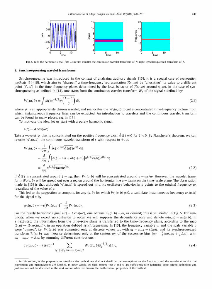
Fig. 5. Left: the harmonic signal f (t) = sin(8t); middle: the continuous wavelet transform of f ; right: synchrosqueezed transform of f .

2. Synchrosqueezing wavelet transforms

Synchrosqueezing was introduced in the context of analyzing auditory signals [13]; it is a special case of reallocationmethods [14–16], which aim to “sharpen” a time-frequency representation R(t,ω) by “allocating” its value to a differentpoint (t′,ω′) in the time–frequency plane, determined by the local behavior of R(t,ω) around (t,ω). In the case of syn-chrosqueezing as defined in [13], one starts from the continuous wavelet transform W s of the signal s defined by2

W s(a,b) =∫

s(t)a−1/2ψ

(t − b

a

)dt, (2.1)

where ψ is an appropriately chosen wavelet, and reallocates the W s(a,b) to get a concentrated time-frequency picture, fromwhich instantaneous frequency lines can be extracted. An introduction to wavelets and the continuous wavelet transformcan be found in many places, e.g. in [17].

To motivate the idea, let us start with a purely harmonic signal,

s(t) = A cos(ωt).

Take a wavelet ψ that is concentrated on the positive frequency axis: ψ(ξ) = 0 for ξ < 0. By Plancherel’s theorem, we canrewrite W s(a,b), the continuous wavelet transform of s with respect to ψ , as

W s(a,b) = 1

2π

∫s(ξ)a1/2ψ(aξ)eibξ dξ

= A

4π

∫ [δ(ξ − ω) + δ(ξ + ω)

]a1/2ψ(aξ)eibξ dξ

= A

4πa1/2ψ(aω)eibω. (2.2)

If ψ(ξ) is concentrated around ξ = ω0, then W s(a,b) will be concentrated around a = ω0/ω. However, the wavelet trans-form W s(a,b) will be spread out over a region around the horizontal line a = ω0/ω on the time–scale plane. The observationmade in [13] is that although W s(a,b) is spread out in a, its oscillatory behavior in b points to the original frequency ω,regardless of the value of a.

This led to the suggestion to compute, for any (a,b) for which W s(a,b) �= 0, a candidate instantaneous frequency ωs(a,b)

for the signal s by

ωs(a,b) = −i(W s(a,b)

)−1 ∂

∂bW s(a,b). (2.3)

For the purely harmonic signal s(t) = A cos(ωt), one obtains ωs(a,b) = ω, as desired; this is illustrated in Fig. 5. For sim-plicity, when we expect no confusion to occur, we will suppress the dependence on s and denote ω(a,b) = ωs(a,b). Ina next step, the information from the time–scale plane is transferred to the time–frequency plane, according to the map(b,a) → (b,ωs(a,b)), in an operation dubbed synchrosqueezing. In [13], the frequency variable ω and the scale variable awere “binned”, i.e. W s(a,b) was computed only at discrete values ak , with ak − ak−1 = (�a)k , and its synchrosqueezedtransform Ts(ω,b) was likewise determined only at the centers ω� of the successive bins [ω� − 1

2 �ω,ω� + 12 �ω], with

ω� − ω�−1 = �ω, by summing different contributions:

Ts(ω�,b) = (�ω)−1∑

ak: |ω(ak,b)−ωl|��ω/2

W s(ak,b)a−3/2k (�a)k. (2.4)

2 In this section, as the purpose is to introduce the method, we shall not dwell on the assumptions on the function s and the wavelet ψ so that theexpressions and manipulations are justified. In other words, we shall assume that s and ψ are sufficiently nice functions. More careful definitions andjustifications will be discussed in the next section when we discuss the mathematical properties of the method.


The following argument shows that the signal can still be reconstructed after the synchrosqueezing. We have

∞∫0

W s(a,b)a−3/2 da = 1

2π

∞∫−∞

∞∫0

s(ξ)ψ(aξ)eibξa−1 da dξ

= 1

2π

∞∫0

∞∫0

s(ξ)ψ(aξ)eibξa−1 da dξ

=∞∫

0

ψ(ξ)dξ

ξ· 1

2π

∞∫0

s(ζ )eibζ dζ. (2.5)

Setting Cψ = 12

∫ ∞0 ψ(ξ)

dξξ

, we then obtain (assuming that s is real, so that s(ξ) = s(−ξ), hence s(b) = π−1Re[∫ ∞0 s(ξ)×

eibξ dξ ])

s(b) = Re

[C−1

ψ

∞∫0

W s(a,b)a−3/2 da

]. (2.6)

In the piecewise constant approximation corresponding to the binning in a, this becomes

s(b) ≈ Re

[C−1

ψ

∑k

W s(ak,b)a−3/2k (�a)k

]= Re

[C−1

ψ

∑�

Ts(ω�,b)(�ω)

]. (2.7)

Remark. As defined above, (2.4) assumes a linear scale discretization of ω. If instead another discretization (e.g., logarithmicdiscretization) is used, the �ω has to be made dependent on �; alternatively, one can also change the exponent of a from−3/2 to −1/2.

If one chooses (as we shall do here) to continue to treat a and ω as continuous variables, without discretization, theanalog of (2.4) is3

Ts(ω,b) =∫

A(b)

W s(a,b)a−3/2δ(ω(a,b) − ω

)da, (2.8)

where A(b) = {a; W s(a,b) �= 0}, and ω(a,b) is as defined in (2.3) above, for (a,b) such that a ∈ A(b).

Remark. In practice, the determination of those (a,b)-pairs for which W s(a,b) = 0 is rather unstable, when s has beencontaminated by noise. For this reason, it is often useful to consider a threshold for |W s(a,b)|, below which ω(a,b) is notdefined; this amounts to replacing A(b) by the smaller region Aε(b) := {a; |W s(a,b)| � ε}.

3. Main result

We define a class of functions, containing intrinsic mode type components that are well separated, and show that they canbe identified and characterized by means of synchrosqueezing.

We start with the following definitions:

Definition 3.1 (Intrinsic mode type function). A continuous function f : R → C, f ∈ L∞(R) is said to be intrinsic-mode-type(IMT) with accuracy ε > 0 if f (t) = A(t)eiφ(t) with A and φ having the following properties:

A ∈ C1(R) ∩ L∞(R), φ ∈ C2(R),

inft∈R

φ′(t) > 0, supt∈R

φ′(t) < ∞,∣∣A′(t)∣∣, ∣∣φ′′(t)

∣∣ � ε∣∣φ′(t)

∣∣, ∀t ∈ R,

M ′′ := supt∈R

∣∣φ′′(t)∣∣ < ∞.

3 The expression δ(ω(a,b) − ω) should be interpreted in the sense of distributions; we will come back to this in the next section.


Definition 3.2 (Superposition of well-separated intrinsic mode components). A function f : R → C is said to be a superpositionof, or to consist of, well-separated intrinsic mode components, up to accuracy ε , and with separation d, if there exists a finite K ,such that

f (t) =K∑

k=1

fk(t) =K∑

k=1

Ak(t)eiφk(t),

where all the fk are IMT, and where moreover their respective phase functions φk satisfy

φ′k(t) > φ′

k−1(t) and∣∣φ′

k(t) − φ′k−1(t)

∣∣ � d[φ′

k(t) + φ′k−1(t)

], ∀t ∈ R.

Remark. It is not really necessary for the components fk to be defined on all of R. One can also suppose that they aresupported on intervals, supp( fk) = supp(Ak) ⊂ [−Tk, Tk], where the different Tk need not be identical. In this case thevarious inequalities governing the definition of an IMT function or a superposition of well-separated IMT components mustsimply be restricted to the relevant intervals. For the inequality above on the φ′

k(t), φ′k−1(t), it may happen that some t

are covered by (say) [−Tk, Tk] but not by [−Tk−1, Tk−1]; one should then replace k − 1 by the largest � < k for whicht ∈ [−T�, T�]; other, similar, changes would have to be made if t ∈ [−Tk−1, Tk−1] \ [−Tk, Tk].

We omit this extra wrinkle for the sake of keeping notations manageable.

Notation (Class Aε,d). We denote by Aε,d the set of all superpositions of well-separated IMT, up to accuracy ε and withseparation d.

Remark. The function class Aε,d defined above is a subset of L∞(R). Note that it is just a set of functions but not a vectorspace: the sum of two elements in Aε,d is still a superposition of IMT components but they could fail to have separation d,in the sense of the definition above.

Our main result is then the following:

Theorem 3.3. Let f be a function in Aε,d, and set ε := ε1/3 . Pick a function h ∈ C∞c with

∫h(t)dt = 1, and pick a wavelet ψ in

Schwartz class such that its Fourier transform ψ is supported in [1 − �,1 + �], with � < d/(1 + d); set Rψ = √2π

∫ψ(ζ )ζ−1 dζ .

Consider the continuous wavelet transform W f (a,b) of f with respect to this wavelet, as well as the function Sδf ,ε (b,ω) obtained by

synchrosqueezing W f , with threshold ε and accuracy δ, i.e.

Sδf ,ε (b,ω) :=

∫Aε, f (b)

W f (a,b)1

δh

(ω − ω f (a,b)

δ

)a−3/2 da, (3.1)

where Aε, f (b) := {a ∈ R+; |W f (a,b)| > ε}. Then, provided ε (and thus also ε) is sufficiently small, the following hold:

• |W f (a,b)| > ε only when, for some k ∈ {1, . . . , K }, (a,b) ∈ Zk := {(a,b); |aφ′k(b) − 1| < �}.

• For each k ∈ {1, . . . , K }, and for each pair (a,b) ∈ Zk for which holds |W f (a,b)| > ε , we have∣∣ω f (a,b) − φ′k(b)

∣∣ � ε.

• Moreover, for each k ∈ {1, . . . , K }, there exists a constant C such that, for any b ∈ R,∣∣∣∣ limδ→0

(R−1

ψ

∫|ω−φ′

k(b)|<ε

Sδf ,ε (b,ω)dω

)− Ak(b)eiφk(b)

∣∣∣∣ � C ε.

The function Sδf ,ε , defined by (3.1), can be viewed as the “action” of the distribution in (2.8) on the Schwartz function

δ−1h(·/δ); in the limit for δ → 0, Sδf ,ε tends, in the sense of distributions, to (2.8). Theorem 3.3 basically tells us that, for

f ∈ Aε,d , the (smoothed) synchrosqueezed version Sδf ,ε of the wavelet transform W f is concentrated, in the (b,ω)-plane, in

narrow bands around the curves ω = φ′k(b), and that the restriction of Sδ

f ,ε to the k-th narrow band suffices to reconstruct,with high precision, the k-th IMT component of f . Synchrosqueezing (an appropriate) wavelet transform thus provides theadaptive time-frequency decomposition that is the goal of empirical mode decomposition.

The proof of Theorem 3.3 relies on a number of estimates, which we demonstrate one by one, at the same time providingmore details about what it means for ε to be “sufficiently small”. In the statement and proof of all the estimates in thissection, we shall always assume that all the conditions of Theorem 3.3 are satisfied (without repeating them), unless statedotherwise.

The first estimate bounds the growth of the Ak , φ′ in the neighborhood of t , in terms of the value of |φ′ (t)|.
k k


Estimate 3.4. For each k ∈ {1, . . . , K }, we have∣∣Ak(t + s) − Ak(t)∣∣ � ε|s|

(∣∣φ′k(t)

∣∣ + 1

2M ′′

k |s|)

and

∣∣φ′k(t + s) − φ′

k(t)∣∣ � ε|s|

(∣∣φ′k(t)

∣∣ + 1

2M ′′

k |s|)

.

Proof. When s � 0, we have (the case s < 0 can be done in an analogue way)

∣∣Ak(t + s) − Ak(t)∣∣ =

∣∣∣∣∣s∫

0

A′k(t + u)du

∣∣∣∣∣�

s∫0

∣∣A′k(t + u)

∣∣du � ε

s∫0

∣∣φ′k(t + u)

∣∣du

= ε

s∫0

∣∣∣∣∣φ′k(t) +

u∫0

φ′′k (t + x)dx

∣∣∣∣∣ du

� ε

(∣∣φ′k(t)

∣∣|s| + 1

2M ′′

k |s|2)

.

The other bound is analogous. �The next estimate shows that, for f and ψ satisfying the conditions in the statement of Theorem 3.3, the wavelet

transform W f (a,b) is concentrated near the regions where, for some k ∈ {1,2, . . . , K }, aφ′k(b) is close to 1. (This estimate is

similar to the argument in stationary phase approximations, for example, used in [18].)

Estimate 3.5.∣∣∣∣∣W f (a,b) − √2π

K∑k=1

Ak(b)eiφk(b)√

aψ(aφ′

k(b))∣∣∣∣∣ � εa3/2Γ1(a,b),

where

Γ1(a,b) := I1

K∑k=1

∣∣φ′k(b)

∣∣ + 1

2I2a

K∑k=1

[M ′′

k + ∣∣Ak(b)∣∣∣∣φ′

k(b)∣∣] + 1

6I3a2

K∑k=1

M ′′k

∣∣Ak(b)∣∣,

with In := ∫ |u|n|ψ(u)|du.

Proof. Since f ∈ Aε,δ ⊂ L∞(R) and ψ ∈ S , the continuous wavelet transform of f with respect to ψ is well defined, andwe have

W f (a,b) =K∑

k=1

∫Ak(t)eiφk(t)a−1/2ψ

(t − b

a

)dt

=K∑

k=1

Ak(b)

∫ei[φk(b)+φ′

k(b)(t−b)+∫ t−b0 [φ′

k(b+u)−φ′k(b)]du]a−1/2ψ

(t − b

a

)dt

+K∑

k=1

∫ [Ak(t) − Ak(b)

]eiφk(t)a−1/2ψ

(t − b

a

)dt.

Using that

√2π Ak(b)eiφk(b)

√aψ

(aφ′

k(b)) = ei(φk(b)−bφ′

k(b))

∫Ak(b)eitφ′

k(b) 1√aψ

(t − b

a

)dt,

we obtain

∣∣∣∣∣W f (a,b) − √2π
K∑k=1

Ak(b)eiφk(b)√

aψ(aφ′

k(b))∣∣∣∣∣

�K∑

k=1

∫ ∣∣Ak(t) − Ak(b)∣∣a−1/2

∣∣∣∣ψ(t − b

a

)∣∣∣∣ dt

+K∑

k=1

∣∣Ak(b)∣∣ ∫ ∣∣ei

∫ t−b0 [φ′

k(b+u)−φ′k(b)]du − 1

∣∣a−1/2∣∣∣∣ψ(

t − b

a

)∣∣∣∣ dt

�K∑

k=1

∫ε|t − b|

(∣∣φ′k(b)

∣∣ + 1

2M ′′

k |t − b|)

a−1/2∣∣∣∣ψ(

t − b

a

)∣∣∣∣dt

+K∑

k=1

∣∣Ak(b)∣∣ ∫ ∣∣∣∣∣

t−b∫0

[φ′

k(b + u) − φ′k(b)

]du

∣∣∣∣∣a−1/2∣∣∣∣ψ(

t − b

a

)∣∣∣∣ dt

� ε

K∑k=1

[a3/2

∣∣φ′k(b)

∣∣ ∫ |u|∣∣ψ(u)∣∣du + a5/2 1

2M ′′

k

∫|u|2∣∣ψ(u)

∣∣du

]

+K∑

k=1

∣∣Ak(b)∣∣ε ∫ [

1

2|t − b|2∣∣φ′

k(b)∣∣ + 1

6|t − b|3M ′′

k

]a−1/2

∣∣∣∣ψ(t − b

a

)∣∣∣∣dt

� εa3/2

{I1

K∑k=1

∣∣φ′k(b)

∣∣ + 1

2I2a

K∑k=1

[M ′′

k + ∣∣Ak(b)∣∣∣∣φ′

k(b)∣∣] + 1

6I3a2

K∑k=1

M ′′k

∣∣Ak(b)∣∣}. � (3.2)

The wavelet ψ satisfies ψ(ξ) �= 0 only for 1 − � < ξ < 1 + �; it follows that |W f (a,b)| � εa3/2Γ1(a,b) whenever|aφ′

k(b) − 1| > � for all k ∈ {1, . . . , K }. On the other hand, we also have the following lemma:

Lemma 3.6. For any pair (a,b) under consideration, there can be at most one k ∈ {1, . . . , K } for which |aφ′k(b) − 1| < �.

Proof. Suppose that k, � ∈ {1, . . . , K } both satisfy the condition, i.e. that |aφ′k(b) − 1| < � and |aφ′

�(b) − 1| < �, with k �= �.For the sake of definiteness, assume k > �. Since f ∈ Aε,d , we have

φ′k(b) − φ′

�(b) � φ′k(b) − φ′

k−1(b) � d[φ′

k(b) + φ′k−1(b)

]� d

[φ′

k(b) + φ′�(b)

].

Combined with

φ′k(b) − φ′

�(b) � a−1[(1 + �) − (1 − �)] = 2a−1�,

φ′k(b) + φ′

�(b) � a−1[(1 − �) + (1 − �)] = 2a−1(1 − �),

this gives

� � d(1 − �),

which contradicts the condition � < d/(1 + d) from Theorem 3.3. �It follows that the (a,b)-plane contains K non-touching “zones” given as Zk = {|aφ′

k(b)−1| < �}, k ∈ {1, . . . , K }, separatedby a “no-man’s land” where |W f (a,b)| is small. Note that the lower and upper bounds on φ′

k(b) imply that the values ofa for which (a,b) ∈ Zk , for some k ∈ {1, . . . , K }, are uniformly bounded from above and from below. It then follows thatΓ1(a,b) is uniformly bounded as well, for (a,b) ∈ ⋃K

k=1 Zk , and that inf{a−9/4Γ−3/2

1 (a,b); (a,b) ∈ ⋃Kk=1 Zk} > 0. We shall

assume (see below) that ε is sufficiently small, i.e., that for all (a,b) ∈ ⋃Kk=1 Zk ,

ε < a−9/4Γ−3/2

1 (a,b), (3.3)

so that εa3/2Γ1(a,b) < ε1/3 = ε . The upper bound in the intermediate region between the zones Zk is then below thethreshold ε allowed for the computation of ω f (a,b) used in S f ,ε (see the formulation of Theorem 3.3). It follows that wewill compute ω f (a,b) only in the special zones themselves. We thus need to estimate ∂b W f (a,b) in each of these zones.


Estimate 3.7. For k ∈ {1, . . . , K }, and (a,b) ∈ R+ × R such that |aφ′k(b) − 1| < �, we have∣∣−i∂b W f (a,b) − √

2π Ak(b)eiφk(b)√

aφ′k(b)ψ

(aφ′

k(b))∣∣ � εa1/2Γ2(a,b),

where

Γ2(a,b) := I ′1K∑

�=1

∣∣φ′�(b)

∣∣ + 1

2I ′2a

K∑�=1

[M ′′

� + ∣∣A�(b)∣∣∣∣φ′

�(b)∣∣] + 1

6I ′3a2

K∑�=1

M ′′�

∣∣A�(b)∣∣,

with I ′n := ∫ |u|n|ψ ′(u)|du.

(Note that, like Γ1, Γ2(a,b) is uniformly bounded for (a,b) ∈ ⋃Kk=1 Zk , by essentially the same argument.)

Proof. The proof follows the same lines as that for Estimate 3.5. Since ψ ∈ S , we obtain (by using the Dominant Conver-gence theorem) that

∂b W f (a,b) = ∂b

(K∑

�=1

∫A�(t)eiφ�(t)a−1/2ψ

(t − b

a

)dt

)

= −K∑

�=1

∫A�(t)eiφ�(t)a−3/2ψ ′

(t − b

a

)dt

= −K∑

�=1

A�(b)

∫ei[φ�(b)+φ′

�(b)(t−b)+∫ t−b0 [φ′

�(b+u)−φ′�(b)]du]a−3/2ψ ′

(t − b

a

)dt

−K∑

�=1

∫ [A�(t) − A�(b)

]eiφ�(t)a−3/2ψ ′

(t − b

a

)dt. (3.4)

By Lemma 3.6, only the term for � = k is nonzero in the sum for (a,b) such that |aφ′k(b) − 1| < �. Also note that


√aφ′

k(b)ψ(aφ′

k(b))

= ei(φk(b)−bφ′k(b))

∫Ak(b)eitφ′

k(b) 1√aψ

(t − b

a

)φ′

k(b)dt

= iei(φk(b)−bφ′k(b))

∫Ak(b)eitφ′

k(b) 1

a3/2ψ ′

(t − b

a

)dt.

Thus for (a,b) such that |aφ′k(b) − 1| < �,

∂b W f (a,b) = −Ak(b)

∫ei[φk(b)+φ′

k(b)(t−b)+∫ t−b0 [φ′

k(b+u)−φ′k(b)]du]a−3/2ψ ′

(t − b

a

)dt

−∫ [

Ak(t) − Ak(b)]eiφk(t)a−3/2ψ ′

(t − b

a

)dt,

and we obtain∣∣∂b W f (a,b) − i√

2π Ak(b)eiφk(b)√

aφ′k(b)ψ

(aφ′

k(b))∣∣

=∣∣∣∣∂b W f (a,b) − √

2π Ak(b)eiφk(b) 1√aψ ′(aφ′

k(b))∣∣∣∣

�K∑

�=1

∫ε|t − b|

(∣∣φ′�(b)

∣∣ + 1

2M ′′|t − b|

)a−3/2

∣∣∣∣ψ ′(

t − b

a

)∣∣∣∣dt

+K∑

�=1

∣∣Ak(b)∣∣ ∫ ∣∣ei

∫ t−b0 [φ′

�(b+u)−φ′�(b)]du − 1

∣∣a−3/2∣∣∣∣ψ ′

(t − b

a

)∣∣∣∣ dt

� ε

K∑[a1/2

∣∣φ′�(b)

∣∣ ∫ |u|∣∣ψ ′(u)∣∣du + a3/2 1

2M ′′

�

∫|u|2∣∣ψ ′(u)

∣∣du

]
�=1


+ ε

K∑�=1

∣∣A�(b)∣∣ ∫ [

1

2|t − b|2∣∣φ′

�(b)∣∣ + 1

6|t − b|3M ′′

�

]a−3/2

∣∣∣∣ψ ′(

t − b

a

)∣∣∣∣ dt

� εa1/2K∑

�=1

{I ′1

∣∣φ′�(b)

∣∣ + 1

2I ′2a

[M ′′

� + ∣∣A�(b)∣∣∣∣φ′

�(b)∣∣] + 1

6I ′3a2M ′′

�

∣∣A�(b)∣∣}. �

Combining Estimates 3.5 and 3.7, we find

Estimate 3.8. Suppose that (3.3) is satisfied. For k ∈ {1, . . . , K }, and (a,b) ∈ R+ ×R such that both |aφ′k(b)−1| < � and W f (a,b) �

ε are satisfied, we have∣∣ω f (a,b) − φ′k(b)

∣∣ �√

a(Γ2 + aΓ1φ

′k(b)

)ε2/3.

Proof. By definition,

ω f (a,b) = −i∂b W f (a,b)

W f (a,b).

For convenience, let us, for this proof only, use the short-hand notation B = √2π Ak(b)eiφk(b)

√aψ(aφ′

k(b)). For the (a,b)-pairs under consideration, we have then∣∣−i∂b W f (a,b) − φ′

k(b)B∣∣ � εa1/2Γ2 and

∣∣W f (a,b) − B∣∣ � εa3/2Γ1.

Using ε = ε1/3, it follows that

ω f (a,b) − φ′k(b) = −i∂b W f (a,b) − φ′

k(b)B

W f (a,b)+ [B − W f (a,b)]φ′

k(b)

W f (a,b),

so that∣∣ω f (a,b) − φ′k(b)

∣∣ �εa1/2Γ2 + εa3/2φ′

k(b)Γ1

W f (a,b)

�√

a(Γ2 + aΓ1φ

′k(b)

)ε2/3. �

If (see below) we impose an extra restriction on ε , namely that, for all k ∈ {1,2, . . . , K } and all (a,b) ∈ {(a,b); |aφ′k(b) −

1| < �, W f (a,b) � ε} ⊂ Zk ,

0 < ε < a−3/2[Γ2(a,b) + aφ′k(b)Γ1(a,b)

]−3(3.5)

(note that the right-hand side is uniformly bounded below, away from zero, for (a,b) ∈ ⋃Kk=1 Zk , guaranteeing the existence

of ε > 0 that can satisfy this inequality), then this last estimate can be simplified to∣∣ω f (a,b) − φ′k(b)

∣∣ < ε. (3.6)

Next is our final estimate:

Estimate 3.9. Suppose that both (3.3) and (3.5) are satisfied, and that, in addition, for all b under consideration,

ε � 1/8d3[φ′1(b) + φ′

2(b)]3

. (3.7)

Let Sδf ,ε be the synchrosqueezed wavelet transform of f with accuracy δ,

Sδf ,ε (b,ω) :=

∫Aε, f (b)

W f (a,b)1

δh

(ω − ω f (a,b)

δ

)a−3/2 da.

Then we have, for all b ∈ R, and all k ∈ {1, . . . , K }∣∣∣∣ limδ→0

R−1ψ

∫|ω−φ′

k(b)|<ε

S f ,ε (b,ω)dω − Ak(b)eiφk(b)

∣∣∣∣ � C ε.


Proof. For later use, note first that (3.7) implies that, for all k, � ∈ {1, . . . , K },

d[φ′

k(b) + φ′�(b)

]> 2ε. (3.8)

For a fixed b ∈ R under consideration, since W f (a,b) ∈ C∞(Aε, f (b)), where Aε, f (b) is inside the compact set⋃K

k=1 Zk awayfrom zero, clearly Sδ

f ,ε (b,ω) ∈ C∞(R). We have

limδ→0

∫|ω−φ′

k(b)|<ε

Sδf ,ε (b,ω)dω = lim

δ→0

∫|ω−φ′

k(b)|<ε

∫Aε, f (b)

W f (a,b)1

δh

(ω − ω f (a,b)

δ

)a−3/2 da dω

= limδ→0

∫Aε, f (b)

a−3/2W f (a,b)

∫|ω−φ′

k(b)|<ε

1

δh

(ω − ω f (a,b)

δ

)dω da

=∫

Aε, f (b)

a−3/2W f (a,b) limδ→0

∫|ω−φ′

k(b)|<ε

1

δh

(ω − ω f (a,b)

δ

)dω da

=∫

Aε, f (b)∩{a;|ω f (a,b)−φ′k(b)|<ε}

W f (a,b)a−3/2 da,

where we have used the Fubini theorem for the second equality, and the Dominant Convergence theorem for the thirdand fourth equalities: the integrand is bounded by a−3/2W f (a,b) ∈ L1(Aε, f (b)) and converges a.e. to a−3/2W f (a,b) if|ω f (a,b) − φ′

k(b)| < ε , and to zero if |ω f (a,b) − φ′k(b)| > ε . From Estimate 3.5 and (3.3) we know that |W f (a,b)| > ε only

when |aφ′�(b) − 1| < � for some � ∈ {1, . . . , K }. When � �= k, we have, by Estimate 3.8, that |aφ′

�(b) − 1| < � implies (use(3.8)) ∣∣ω f (a,b) − φ′

k(b)∣∣ �

∣∣φ′�(b) − φ′

k(b)∣∣ − ∣∣ω f (a,b) − φ′

�(b)∣∣

� d[φ′

�(b) + φ′k(b)

] − ε > ε.

It follows that there is only one � for which |aφ′�(b) − 1| < � and |ω f (a,b)| − φ′

k(b)| < ε hold simultaneously, namely � = k.Hence

limδ→0

∫|ω−φ′

k(b)|<ε

Sδf ,ε (b,ω)dω =

∫Aε, f (b)∩{|aφ′

k(b)−1|<�}W f (a,b)a−3/2 da

=( ∫

|aφ′k(b)−1|<�

W f (a,b)a−3/2 da

)−

( ∫{|aφ′

k(b)−1|<�}\Aε, f (b)

W f (a,b)a−3/2 da

).

From Estimate 3.5 we then obtain∣∣∣∣ limδ→0

R−1ψ

∫|ω−φ′

k(b)|<ε

Sδf ,ε (b,ω)dω − Ak(b)eiφk(b)

∣∣∣∣�

∣∣∣∣R−1ψ

( ∫|aφ′

k(b)−1|<�

W f (a,b)a−3/2 da

)− Ak(b)eiφk(b)

∣∣∣∣ + R−1ψ

∣∣∣∣ ∫{|aφ′

k(b)−1|<�}\Aε, f (b)

W f (a,b)a−3/2 da

∣∣∣∣�

∣∣∣∣R−1ψ


( ∫|aφ′

k(b)−1|<�

√aψ

(aφ′

k(b))a−3/2 da

)− Ak(b)eiφk(b)

∣∣∣∣+ R−1

ψ

∫|aφ′

k(b)−1|<�

[ε + εa−3/2] da.

The first term on the right-hand side vanishes, since

R−1ψ


∫|aφ′

k(b)−1|<�

ψ(aφ′

k(b))a−1 da

= R−1ψ


∫ψ(ζ )ζ−1 dζ = Ak(b)eiφk(b),

|ζ−1|<�


by the definition of Rψ . In the second term, the integrals can be worked out explicitly. We thus obtain∣∣∣∣ limδ→0

R−1ψ

∫|ω−φ′

k(b)|<ε

Sδf ,ε (t,ω)dω − Ak(b)eiφk(b)

∣∣∣∣ � 2εR−1ψ

[�

φ′k(b)

+(

φ′k(b)

1 − �

)1/2

−(

φ′k(b)

1 + �

)1/2]. �

It is now easy to see that all the estimates together provide a complete proof for Theorem 3.3.

Remark. We have three different conditions on ε , namely (3.3), (3.5) and (3.7). The auxiliary quantities in these inequalitiesdepend on a and b, and the conditions should be satisfied for all (a,b)-pairs under consideration. This is not really aproblem: we saw that the conditions on Ak(b) and φ′

k(b) imply that there exists an interval of positive measure in whichall elements satisfy the three conditions. Note that the different terms can be traded off in many other ways than what isdone here; no effort has been made to optimize the bounds, and they can surely be improved. The focus here was not onoptimizing the constants, but on proving that, if the rate of change (in time) of the Ak(b) and the φ′

k(b) is small, comparedwith the rate of change of the φk(b) themselves, then synchrosqueezing will identify both the “instantaneous frequencies”and their amplitudes.

In the statement of Theorem 3.3, we required the wavelet ψ to be in Schwartz class and have a compactly supportedFourier transform. These assumptions are not absolutely necessary; it was done here for convenience in the proof. Forexample, if ψ is not compactly supported, then extra terms occur in many of the estimates, taking into account the decayof ψ(ζ ) as ζ → ∞ or ζ → 0; these can be handled in ways similar to what we saw above, at the cost of significantlylengthening the computations without making a conceptual difference.

4. A variational approach

The construction and estimates in this section can also be interpreted in a variational framework.Let us go back to the notion of “instantaneous frequency”. Consider a signal s(t) that is a sum of IMT components si(t):

s(t) =N∑

i=1

si(t) =N∑

i=1

Ai(t) cos(φi(t)

), (4.1)

with the additional constraints that φ′i(t) and φ′

j(t) for i �= j are “well separated”, so that it is reasonable to considerthe si as individual components. According to the philosophy of EMD, the instantaneous frequency at time t , for the i-thcomponent, is then given by ωi(t) = φ′

i(t).How could we use this to build a time-frequency representation for s? If we restrict ourselves to a small window in time

around T , of the type [T − �t, T + �t], with �t ≈ 2π/φ′i(T ), then (by its IMT nature) the i-th component can be written

(approximately) as

si(t)|[T −�t,T +�t] ≈ Ai(T ) cos[φi(T ) + φ′

i(T )(t − T )],

which is essentially a truncated Taylor expansion in which terms on the order O(A′i(T )), O(φ′′

i (T )) have been neglected.Introducing ωi(T ) = φ′

i(T ), and the phase ϕi(T ) := φi(T ) − ωi(T )T we can rewrite this as

si(t)|[T −�t,T +�t] ≈ Ai(T ) cos[ωi(T )t + ϕi(T )

].

This signal has a time-frequency representation, as a bivariate “function” of time and frequency, given by (for t ∈ [T −�t, T + �t])

Fi(t,ω) = Ai(T ) cos[ωt + ϕi(T )

]δ(ω − ωi(T )

), (4.2)

where δ is the Dirac-delta measure. The time-frequency representation for the full signal s = ∑Ni=1 si , still in the neighbor-

hood of t = T , would then be

F (t,ω) =N∑

i=1

Ai(T ) cos[ωt + ϕi(T )

]δ(ω − ωi(T )

). (4.3)

Integrating over ω, in the neighborhood of t = T , leads to s(t) ≈ ∫F (t,ω)dω.

All this becomes even simpler if we introduce the “complex form” of the time-frequency representation: for t near T ,we have

F (t,ω) =N∑

A j(T )exp(iωt)δ(ω − φ′

j(T )),

j=1


with A j(T ) = A j(T )exp[iϕ j(T )]; integration over ω now leads to

Re

[∫F (t,ω)dω

]= Re

[N∑

j=1

A j(T )exp[iω j(T )t + iϕ j(T )

]] ≈ s(t). (4.4)

Note that, because of the presence of the δ-measure, and under the assumption that the components remain separated, thetime-frequency function F (t,ω) satisfies the equation

∂t F (t,ω) = iω F (t,ω). (4.5)

To get a representation over a longer time interval, the small pieces described above have to be knitted together. One wayof doing this is to set F (t,ω) = ∑N

j=1 A j(t)exp(iωt)δ(ω − ω j(t)). This more globally defined F (t,ω) is still supported onthe N curves given by ω = ω j(t), corresponding to the instantaneous frequency “profile” of the different components. Thecomplex “amplitudes” A j(t) are given by A j(t) = A j(t)exp[iϕ j(t)], where, to determine the phases exp[iϕ j(t)], it suffices toknow them at one time t0. We have indeed

dϕ j(t)

dt= d

dt

[φ j(t) − ω j(t)t

] = φ′j(t) − ω j(t) − ω′

j(t)t = −ω′j(t)t;

since the ω j(t) are known (they are encoded in the support of F ), we can compute the ϕ j(t) by using

ϕ j(t) = −t∫

t0

ω′j(τ )τ dτ + ϕ j(t0).

Moreover, (4.5) still holds (in the sense of distributions) up to terms of size O(A′i(T )), O(φ′′

i (T )), since

∂t F (t,ω) =N∑

j=1

[A′

j(t) − iω′j(t)t A j(t) + iωA j(t)

]eiωtδ

(ω − ω j(t)

) + A j(t)eiωtω′j(t)δ

′(ω − ω j(t))

= iωN∑

j=1

A j(t)eiωtδ(ω − ω j(t)

) + O(

A′i(T ),φ′′

i (T ))

= iω F (t,ω) + O(

A′i(T ),φ′′

i (T )).

This suggests modeling the adaptive time-frequency decomposition as a variational problem in which one seeks tominimize∫ ∣∣∣∣Re

[∫F (t,ω)dω

]− s(t)

∣∣∣∣2

dt + μ

∫ ∫ ∣∣∂t F (t,ω) − iωF (t,ω)∣∣2

dt dω (4.6)

to which extra terms could be added, such as, γ∫∫ |F (t,ω)|2 dt dω (corresponding to the constraint that F ∈ L2(R2)), or

λ∫ [∫ |F (t,ω)|dω]2 dt (corresponding to a sparsity constraint in ω for each value of t). Using estimates similar to those in

Section 3, one can prove that if s ∈ Aε,d , then its synchrosqueezed wavelet transform Ss,ε (b,ω) is close to the minimizerof (4.6). Because the estimates and techniques of proof are essentially the same as in Section 3, we don’t give the details ofthis analysis here.

Note that wavelets or wavelet transforms play no role in the variational functional – this fits with our numerical obser-vation that although the wavelet transform itself of s is definitely influenced by the choice of ψ , the dependence on ψ is(almost) completely removed when one considers the synchrosqueezed wavelet transform, at least for signals in Aε,d .

5. Numerical results

In this section we illustrate the effectiveness of synchrosqueezed wavelet transforms on several examples. For all theexamples in this section, synchrosqueezing was carried out starting from a Morlet wavelet transform; other wavelets thatare well localized in frequency give similar results. The code of synchrosqueezing is available upon requests to the authors.

5.1. Instantaneous frequency profiles for synthesized data

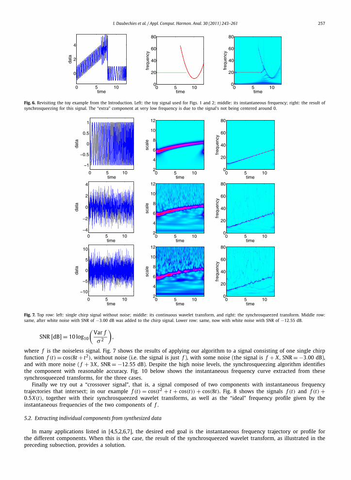
We start by revisiting the toy signal of Figs. 1 and 2 in the Introduction. Fig. 6 shows the result of synchrosqueezingthe wavelet transform of this toy signal. We next explore the tolerance to noise of synchrosqueezed wavelet transforms. Wedenote by X(t) a white noise with zero mean and variance σ 2 = 1. The Signal-to-Noise Ratio (SNR) (measured in dB), will bedefined (as usual) by


Fig. 6. Revisiting the toy example from the Introduction. Left: the toy signal used for Figs. 1 and 2; middle: its instantaneous frequency; right: the result ofsynchrosqueezing for this signal. The “extra” component at very low frequency is due to the signal’s not being centered around 0.

Fig. 7. Top row: left: single chirp signal without noise; middle: its continuous wavelet transform, and right: the synchrosqueezed transform. Middle row:same, after white noise with SNR of −3.00 dB was added to the chirp signal. Lower row: same, now with white noise with SNR of −12.55 dB.

SNR [dB] = 10 log10

(Var f

σ 2

),

where f is the noiseless signal. Fig. 7 shows the results of applying our algorithm to a signal consisting of one single chirpfunction f (t) = cos(8t + t2), without noise (i.e. the signal is just f ), with some noise (the signal is f + X , SNR = −3.00 dB),and with more noise ( f + 3X , SNR = −12.55 dB). Despite the high noise levels, the synchrosqueezing algorithm identifiesthe component with reasonable accuracy. Fig. 10 below shows the instantaneous frequency curve extracted from thesesynchrosqueezed transforms, for the three cases.

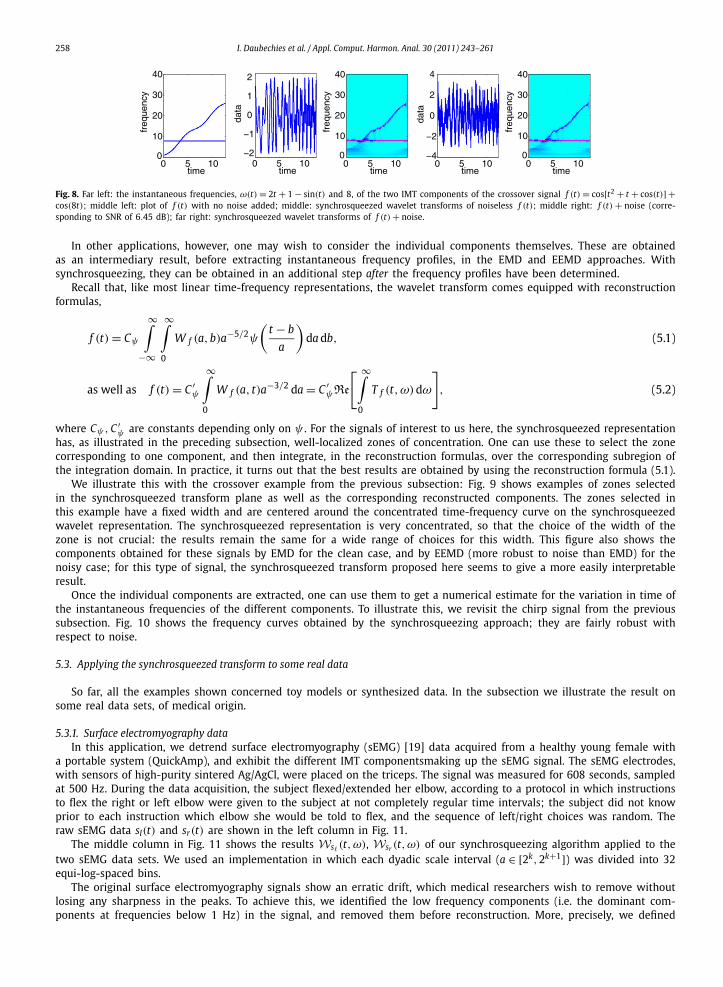
Finally we try out a “crossover signal”, that is, a signal composed of two components with instantaneous frequencytrajectories that intersect; in our example f (t) = cos(t2 + t + cos(t)) + cos(8t). Fig. 8 shows the signals f (t) and f (t) +0.5X(t), together with their synchrosqueezed wavelet transforms, as well as the “ideal” frequency profile given by theinstantaneous frequencies of the two components of f .

5.2. Extracting individual components from synthesized data

In many applications listed in [4,5,2,6,7], the desired end goal is the instantaneous frequency trajectory or profile forthe different components. When this is the case, the result of the synchrosqueezed wavelet transform, as illustrated in thepreceding subsection, provides a solution.


Fig. 8. Far left: the instantaneous frequencies, ω(t) = 2t + 1 − sin(t) and 8, of the two IMT components of the crossover signal f (t) = cos[t2 + t + cos(t)] +cos(8t); middle left: plot of f (t) with no noise added; middle: synchrosqueezed wavelet transforms of noiseless f (t); middle right: f (t) + noise (corre-sponding to SNR of 6.45 dB); far right: synchrosqueezed wavelet transforms of f (t) + noise.

In other applications, however, one may wish to consider the individual components themselves. These are obtainedas an intermediary result, before extracting instantaneous frequency profiles, in the EMD and EEMD approaches. Withsynchrosqueezing, they can be obtained in an additional step after the frequency profiles have been determined.

Recall that, like most linear time-frequency representations, the wavelet transform comes equipped with reconstructionformulas,

f (t) = Cψ

∞∫−∞

∞∫0

W f (a,b)a−5/2ψ

(t − b

a

)da db, (5.1)

as well as f (t) = C ′ψ

∞∫0

W f (a, t)a−3/2 da = C ′ψRe

[ ∞∫0

T f (t,ω)dω

], (5.2)

where Cψ, C ′ψ are constants depending only on ψ . For the signals of interest to us here, the synchrosqueezed representation

has, as illustrated in the preceding subsection, well-localized zones of concentration. One can use these to select the zonecorresponding to one component, and then integrate, in the reconstruction formulas, over the corresponding subregion ofthe integration domain. In practice, it turns out that the best results are obtained by using the reconstruction formula (5.1).

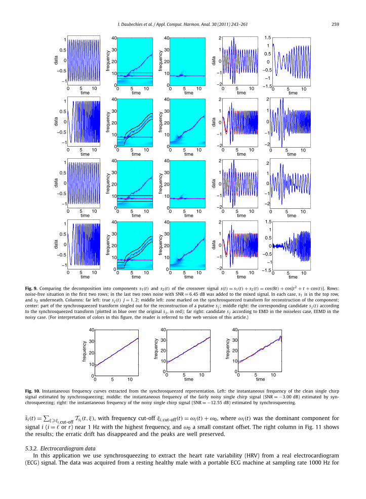
We illustrate this with the crossover example from the previous subsection: Fig. 9 shows examples of zones selectedin the synchrosqueezed transform plane as well as the corresponding reconstructed components. The zones selected inthis example have a fixed width and are centered around the concentrated time-frequency curve on the synchrosqueezedwavelet representation. The synchrosqueezed representation is very concentrated, so that the choice of the width of thezone is not crucial: the results remain the same for a wide range of choices for this width. This figure also shows thecomponents obtained for these signals by EMD for the clean case, and by EEMD (more robust to noise than EMD) for thenoisy case; for this type of signal, the synchrosqueezed transform proposed here seems to give a more easily interpretableresult.

Once the individual components are extracted, one can use them to get a numerical estimate for the variation in time ofthe instantaneous frequencies of the different components. To illustrate this, we revisit the chirp signal from the previoussubsection. Fig. 10 shows the frequency curves obtained by the synchrosqueezing approach; they are fairly robust withrespect to noise.

5.3. Applying the synchrosqueezed transform to some real data

So far, all the examples shown concerned toy models or synthesized data. In the subsection we illustrate the result onsome real data sets, of medical origin.

5.3.1. Surface electromyography dataIn this application, we detrend surface electromyography (sEMG) [19] data acquired from a healthy young female with

a portable system (QuickAmp), and exhibit the different IMT componentsmaking up the sEMG signal. The sEMG electrodes,with sensors of high-purity sintered Ag/AgCl, were placed on the triceps. The signal was measured for 608 seconds, sampledat 500 Hz. During the data acquisition, the subject flexed/extended her elbow, according to a protocol in which instructionsto flex the right or left elbow were given to the subject at not completely regular time intervals; the subject did not knowprior to each instruction which elbow she would be told to flex, and the sequence of left/right choices was random. Theraw sEMG data sl(t) and sr(t) are shown in the left column in Fig. 11.

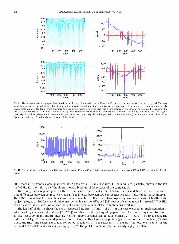
The middle column in Fig. 11 shows the results Ws� (t,ω), Wsr (t,ω) of our synchrosqueezing algorithm applied to thetwo sEMG data sets. We used an implementation in which each dyadic scale interval (a ∈ [2k,2k+1]) was divided into 32equi-log-spaced bins.

The original surface electromyography signals show an erratic drift, which medical researchers wish to remove withoutlosing any sharpness in the peaks. To achieve this, we identified the low frequency components (i.e. the dominant com-ponents at frequencies below 1 Hz) in the signal, and removed them before reconstruction. More, precisely, we defined


Fig. 9. Comparing the decomposition into components s1(t) and s2(t) of the crossover signal s(t) = s1(t) + s2(t) = cos(8t) + cos[t2 + t + cos(t)]. Rows:noise-free situation in the first two rows; in the last two rows noise with SNR = 6.45 dB was added to the mixed signal. In each case, s1 is in the top row,and s2 underneath. Columns: far left: true s j(t) j = 1,2; middle left: zone marked on the synchrosqueezed transform for reconstruction of the component;center: part of the synchrosqueezed transform singled out for the reconstruction of a putative s j ; middle right: the corresponding candidate s j(t) accordingto the synchrosqueezed transform (plotted in blue over the original s j , in red); far right: candidate s j according to EMD in the noiseless case, EEMD in thenoisy case. (For interpretation of colors in this figure, the reader is referred to the web version of this article.)

Fig. 10. Instantaneous frequency curves extracted from the synchrosqueezed representation. Left: the instantaneous frequency of the clean single chirpsignal estimated by synchrosqueezing; middle: the instantaneous frequency of the fairly noisy single chirp signal (SNR = −3.00 dB) estimated by syn-chrosqueezing; right: the instantaneous frequency of the noisy single chirp signal (SNR = −12.55 dB) estimated by synchrosqueezing.

si(t) = ∑ξ�ξi,cut-off

Tsi (t, ξ), with frequency cut-off ξi,cut-off(t) = ωi(t) + ω0, where ωi(t) was the dominant component for

signal i (i = � or r) near 1 Hz with the highest frequency, and ω0 a small constant offset. The right column in Fig. 11 showsthe results; the erratic drift has disappeared and the peaks are well preserved.

5.3.2. Electrocardiogram dataIn this application we use synchrosqueezing to extract the heart rate variability (HRV) from a real electrocardiogram

(ECG) signal. The data was acquired from a resting healthy male with a portable ECG machine at sampling rate 1000 Hz for


Fig. 11. The surface electromyography data described in the text. The erratic (and different) drifts present in these signals are pretty typical. The veryshort-lived peaks correspond to the elbow-flexes by the subject. Left column: the synchrosqueezing transforms of the surface electromyography signals.Coarse scales are near the top of these diagrams, finer scales are shown lower. The peaks are clearly marked over a range of fine scales. Right column: thered curve give the signals “sans drift”, reconstructed by deleting the low frequency region in the synchrosqueezed transforms; comparison with the originalsEMG signals (in blue) shows the R peaks are as sharp as in the original signals, and at precisely the same location. (For interpretation of colors in thisfigure, the reader is referred to the web version of this article.)

Fig. 12. The raw electrocardiogram data. Left: portion between 300 and 400 sec; right: blow-up of the stretch between 320 and 340 sec, with the R peaksmarked.

600 seconds. The samples were quantized at 12 bits across ±10 mV. The raw ECG data e(t) are (partially) shown in the lefthalf of Fig. 12; the right half of the figure shows a blow-up of 20 seconds of the same signal.

The strong, fairly regular spikes in the ECG are called the R peaks; the HRV time series is defined as the sequence oftime differences between consecutive R peaks. (The interval between two consecutive R peaks is also called the RR interval.)The HRV is important for both clinical and basic research; it reflects the physiological dynamics and state of health of thesubject. (See, e.g., [20] for clinical guidelines pertaining to the HRV, and [21] recent advances made in research.) The HRVcan be viewed as a succession of snapshots of an averaged version of the instantaneous heart rate.

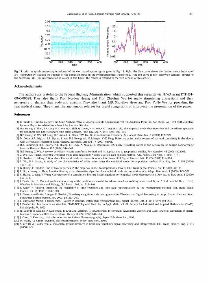
The left half of Fig. 13 shows the synchrosqueezed transform Te(ω, t) of e(t); in this case we used an implementation inwhich each dyadic scale interval (a ∈ [2k,2k+1]) was divided into 128 equi-log-spaced bins. The synchrosqueezed transformTe(ω, t) has a dominant line c(t) near 1.2 Hz, the support of which can be parameterized as {(t,ωc(t)); t ∈ [0.80 sec]}. Theright half of Fig. 13 tracks the dependence on t of ωc(t). This figure also plots a (piecewise constant) function f (t) thattracks the HRV time series and that is computed as follows: if t lies between t − i and ti+1, the locations in time for thei-th and (i + 1)-st R peaks, then f (t) = [ti+1 − ti]−1. The plot for ω(t) and f (t) are clearly highly correlated.


Fig. 13. Left: the synchrosqueezing transforms of the electrocardiogram signals given in Fig. 12. Right: the blue curve shows the “instantaneous heart rate”ω(t) computed by tracking the support of the dominant curve in the synchrosqueezed transform Te ; the red curve is the (piecewise constant) inverse ofthe successive RRi . (For interpretation of colors in this figure, the reader is referred to the web version of this article.)

Acknowledgments

The authors are grateful to the Federal Highway Administration, which supported this research via FHWA grant DTFH61-08-C-00028. They also thank Prof. Norden Huang and Prof. Zhaohua Wu for many stimulating discussions and theirgenerosity in sharing their code and insights. They also thank MD. Shu-Shya Hseu and Prof. Yu-Te Wu for providing thereal medical signal. They thank the anonymous referees for useful suggestions of improving the presentation of the paper.

References

[1] P. Flandrin, Time-Frequency/Time-Scale Analysis, Wavelet Analysis and Its Applications, vol. 10, Academic Press Inc., San Diego, CA, 1999, with a prefaceby Yves Meyer, translated from French by Joachim Stöckler.

[2] N.E. Huang, Z. Shen, S.R. Long, M.C. Wu, H.H. Shih, Q. Zheng, N.-C. Yen, C.C. Tung, H.H. Liu, The empirical mode decomposition and the Hilbert spectrumfor nonlinear and non-stationary time series analysis, Proc. Roy. Soc. A 454 (1998) 903–995.

[3] N.E. Huang, Z. Wu, S.R. Long, K.C. Arnold, K. Blank, T.W. Liu, On instantaneous frequency, Adv. Adapt. Data Anal. 1 (2009) 177–229.[4] M. Costa, A.A. Priplata, L.A. Lipsitz, Z. Wu, N.E. Huang, A.L. Goldberger, C.-K. Peng, Noise and poise: enhancement of postural complexity in the elderly

with a stochastic-resonance-based therapy, Europhys. Lett. EPL 77 (2007) 68008.[5] D.A. Cummings, R.A. Irizarry, N.E. Huang, T.P. Endy, A. Nisalak, K. Ungchusak, D.S. Burke, Travelling waves in the occurrence of dengue haemorrhagic

fever in Thailand, Nature 427 (2004) 344–347.[6] N.E. Huang, Z. Wu, A review on Hilbert–Huang transform: Method and its applications to geophysical studies, Rev. Geophys. 46 (2008) RG2006.[7] Z. Wu, N.E. Huang, Ensemble empirical mode decomposition: A noise-assisted data analysis method, Adv. Adapt. Data Anal. 1 (2009) 1–41.[8] P. Flandrin, G. Rilling, P. Goncalves, Empirical mode decomposition as a filter bank, IEEE Signal Process. Lett. 11 (2) (2004) 112–114.[9] Z. Wu, N.E. Huang, A study of the characteristics of white noise using the empirical mode decomposition method, Proc. Roy. Soc. A 460 (2004)

1597–1611.[10] G. Rilling, P. Flandrin, One or two frequencies? The empirical mode decomposition answers, IEEE Trans. Signal Process. 56 (1) (2008) 85–95.[11] L. Lin, Y. Wang, H. Zhou, Iterative filtering as an alternative algorithm for empirical mode decomposition, Adv. Adapt. Data Anal. 1 (2009) 543–560.[12] C. Huang, L. Yang, Y. Wang, Convergence of a convolution-filtering-based algorithm for empirical mode decomposition, Adv. Adapt. Data Anal. 1 (2009)

560–571.[13] I. Daubechies, S. Maes, A nonlinear squeezing of the continuous wavelet transform based on auditory nerve models, in: A. Aldroubi, M. Unser (Eds.),

Wavelets in Medicine and Biology, CRC Press, 1996, pp. 527–546.[14] F. Auger, P. Flandrin, Improving the readability of time-frequency and time-scale representations by the reassignment method, IEEE Trans. Signal

Process. 43 (5) (1995) 1068–1089.[15] E. Chassande-Mottin, F. Auger, P. Flandrin, Time-frequency/time-scale reassignment, in: Wavelets and Signal Processing, in: Appl. Numer. Harmon. Anal.,

Birkhäuser Boston, Boston, MA, 2003, pp. 233–267.[16] E. Chassande-Mottin, I. Daubechies, F. Auger, P. Flandrin, Differential reassignment, IEEE Signal Process. Lett. 4 (10) (1997) 293–294.[17] I. Daubechies, Ten Lectures on Wavelets, CBMS-NSF Regional Conf. Ser. in Appl. Math., vol. 61, Society for Industrial and Applied Mathematics (SIAM),

Philadelphia, PA, 1992.[18] N. Delprat, B. Escudie, P. Guillemain, R. Kronland-Martinet, P. Tchamitchian, B. Torresani, Asymptotic wavelet and Gabor analysis: extraction of instan-

taneous frequencies, IEEE Trans. Inform. Theory 38 (2) (1992) 644–664.[19] J. Cram, G. Kasman, J. Holtz, Introduction to Surface Electromyography, Aspen Publishers Inc., 1998.[20] M. Malik, A.J. Camm, Dynamic Electrocardiography, Wiley, New York, 2004.[21] S. Cerutti, A. Goldberger, Y. Yamamoto, Recent advances in heart rate variability signal processing and interpretation, IEEE Trans. Biomed. Eng. 53 (1)

(2006) 1–3.

Documents

Synchrosqueezed wavelet transforms: An empirical mode ... · function, or the wavelet transform, where the templates are obtained by translating and dilating the basic (or “mother”)