Synthesizing Electrical and Thermal Load Profiles for Non ... · Master Thesis Presentation Wael A. Al-Qubati Renewable Energy and Energy Eﬃciency for the Middle East and North

Synthesizing Electrical and Thermal Load Profiles forNon-Residential Buildings in Germany

Master Thesis Presentation

Wael A. Al-Qubati

Renewable Energy and Energy Efficiency for the Middle East and North Africa Region [REMENA]University of Kassel

Apr. 08, 2019

Wael A. Al-Qubati Synthetic Load Profile Apr. 08, 2019 1 / 28

Table of Contents

Table of Contents

1 Introduction

2 Methodology

3 Results

4 Conclusions and Outlook


Introduction

Table of Contents

1 IntroductionMotivationThesis Contribution

2 Methodology

3 Results



Introduction Motivation

Motivation

Energy consumption of non-residential sector, trade, commerce and services(TCS), amounted up to 401 TWh in 2017 (15.6% of the total energy demand inGermany) [3].

Majority of existing models for electrical and thermal load profiles: Residentialsector [7].

Lack of information regarding the energy demand of the non-residential sector [1].

Necessity for the stability of the supply and network management.

Optimal integration of new efficient technologies in non-residential buildings.


Introduction Thesis Contribution

Thesis Contribution

Create a model to synthesize individualized electrical and thermal load profiles fornon-residential buildings in 15 minutes resolution.

Takes into account the influence of the behavioural (occupancy, equipment use,etc.) and calendar (holidays, weekdays, seasons, etc.) effects on the load.


Methodology

Table of Contents

1 Introduction

2 MethodologyWork FlowchartElectrical ModelThermal Model

3 Results



Methodology Work Flowchart

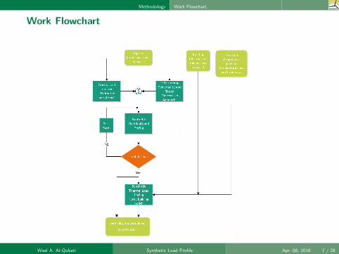
Work Flowchart


Methodology Electrical Model

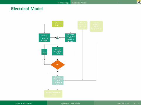
Electrical Model



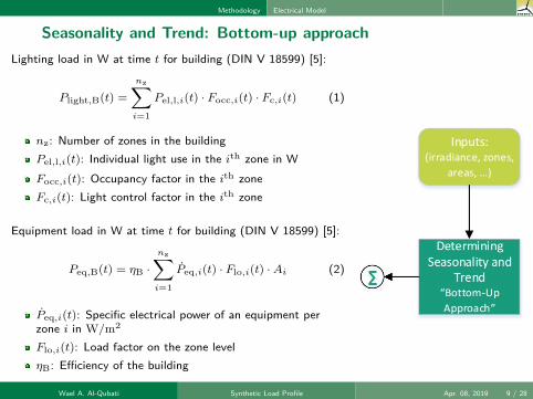
Seasonality and Trend: Bottom-up approachLighting load in W at time t for building (DIN V 18599) [5]:

Plight,B(t) =nz∑i=1

Pel,l,i(t) · Focc,i(t) · Fc,i(t) (1)

nz: Number of zones in the buildingPel,l,i(t): Individual light use in the ith zone in WFocc,i(t): Occupancy factor in the ith zoneFc,i(t): Light control factor in the ith zone

Equipment load in W at time t for building (DIN V 18599) [5]:

Peq,B(t) = ηB ·nz∑i=1

Peq,i(t) · Flo,i(t) ·Ai (2)

Peq,i(t): Specific electrical power of an equipment perzone i in W/m2

Flo,i(t): Load factor on the zone levelηB: Efficiency of the building



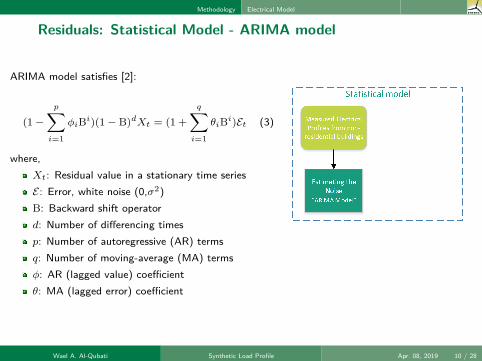
Residuals: Statistical Model - ARIMA model

ARIMA model satisfies [2]:

(1−p∑i=1

φiBi)(1− B)dXt = (1 +q∑i=1

θiBi)Et (3)

where,Xt: Residual value in a stationary time seriesE: Error, white noise (0,σ2)B: Backward shift operatord: Number of differencing timesp: Number of autoregressive (AR) termsq: Number of moving-average (MA) termsφ: AR (lagged value) coefficientθ: MA (lagged error) coefficient



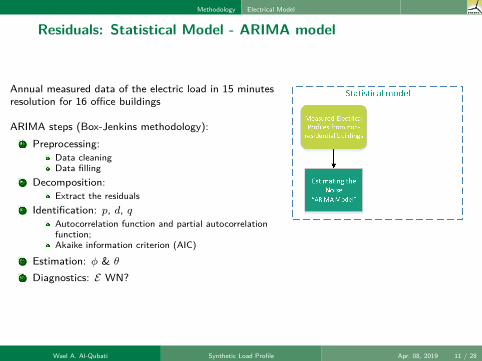
Residuals: Statistical Model - ARIMA model

Annual measured data of the electric load in 15 minutesresolution for 16 office buildings

ARIMA steps (Box-Jenkins methodology):1 Preprocessing:

Data cleaningData filling

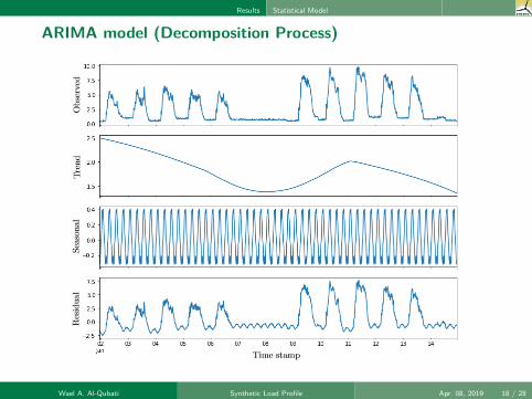
2 Decomposition:Extract the residuals

3 Identification: p, d, qAutocorrelation function and partial autocorrelationfunction;Akaike information criterion (AIC)

4 Estimation: φ & θ

5 Diagnostics: E WN?



Residuals: Statistical Model - Regression Model

For each building i ∈ {1, . . . , N}, regression analysiscan be defined as a column vector [6]:

ai = C · bi + d (4)

where,ai: ARIMA model coefficients;bi: Building’s parameters;C: Estimated regression coefficients;d: Disturbances vector.



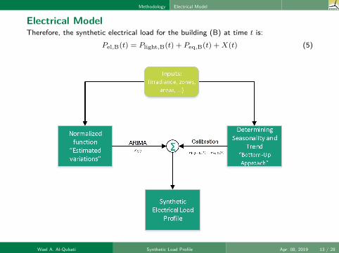
Electrical ModelTherefore, the synthetic electrical load for the building (B) at time t is:

Pel,B(t) = Plight,B(t) + Peq,B(t) +X(t) (5)



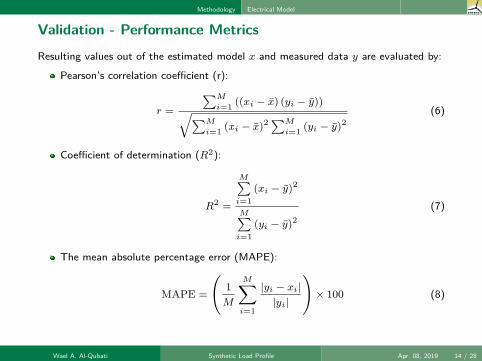
Validation - Performance Metrics

Resulting values out of the estimated model x and measured data y are evaluated by:

Pearson’s correlation coefficient (r):

r =

∑M

i=1 ((xi − x) (yi − y))√∑M

i=1 (xi − x)2∑M

i=1 (yi − y)2(6)

Coefficient of determination (R2):

R2 =

M∑i=1

(xi − y)2

M∑i=1

(yi − y)2(7)

The mean absolute percentage error (MAPE):

MAPE =

(1M

M∑i=1

|yi − xi||yi|

)× 100 (8)


Methodology Thermal Model

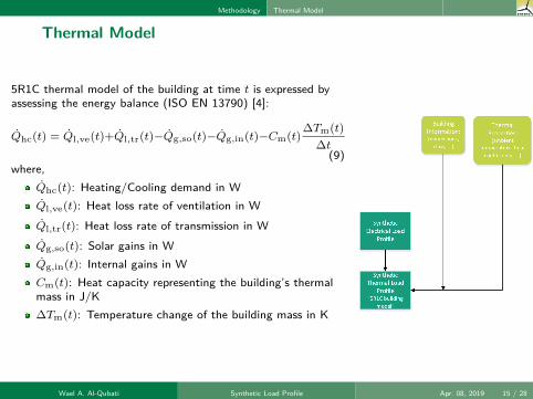
Thermal Model

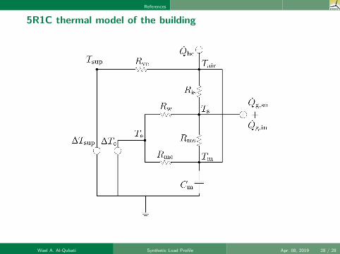
5R1C thermal model of the building at time t is expressed byassessing the energy balance (ISO EN 13790) [4]:

Qhc(t) = Ql,ve(t)+Ql,tr(t)−Qg,so(t)−Qg,in(t)−Cm(t)∆Tm(t)

∆t(9)

where,Qhc(t): Heating/Cooling demand in WQl,ve(t): Heat loss rate of ventilation in WQl,tr(t): Heat loss rate of transmission in WQg,so(t): Solar gains in WQg,in(t): Internal gains in WCm(t): Heat capacity representing the building’s thermalmass in J/K∆Tm(t): Temperature change of the building mass in K


Results

Table of Contents

1 Introduction

2 Methodology

3 ResultsBottom-up ApproachStatistical ModelValidationThermal Model



Results Bottom-up Approach

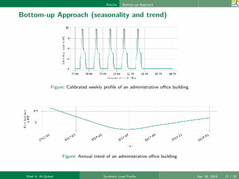
Bottom-up Approach (seasonality and trend)

Figure: Calibrated weekly profile of an administrative office building

Figure: Annual trend of an administrative office building


Results Statistical Model

ARIMA model (Decomposition Process)



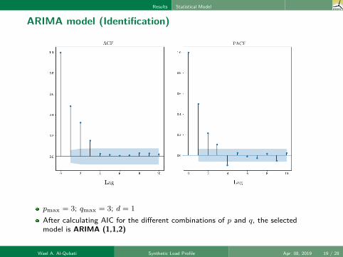
ARIMA model (Identification)

pmax = 3; qmax = 3; d = 1After calculating AIC for the different combinations of p and q, the selectedmodel is ARIMA (1,1,2)



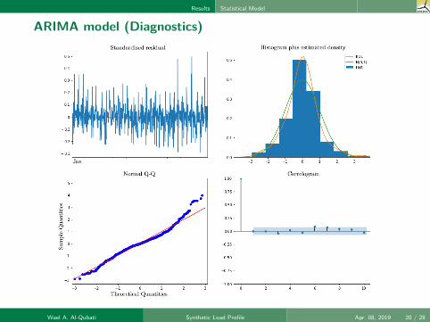
ARIMA model (Diagnostics)


Results Validation

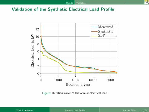
Validation of the Synthetic Electrical Load Profile

Figure: Duration curve of the annual electrical load


Results Validation


Figure: Comparison of one week load profiles


Results Validation


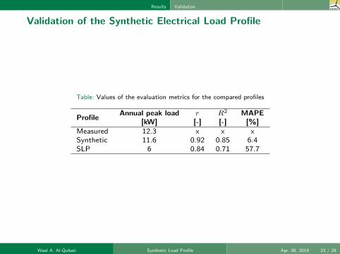
Table: Values of the evaluation metrics for the compared profiles

Profile Annual peak load[kW]

r[-]

R2

[-]MAPE

[%]Measured 12.3 x x xSynthetic 11.6 0.92 0.85 6.4SLP 6 0.84 0.71 57.7


Results Thermal Model

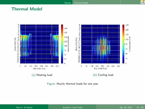
Thermal Model

(a) Heating load (b) Cooling load

Figure: Hourly thermal loads for one year


Results Thermal Model

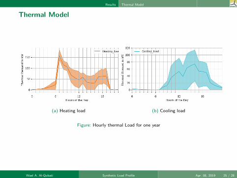
Thermal Model

(a) Heating load (b) Cooling load

Figure: Hourly thermal Load for one year


Conclusions and Outlook

Table of Contents

1 Introduction

2 Methodology

3 Results




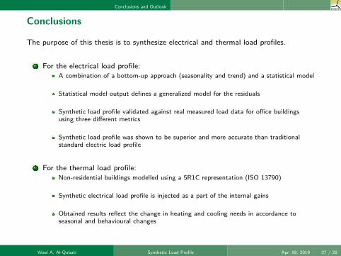
Conclusions

The purpose of this thesis is to synthesize electrical and thermal load profiles.

1 For the electrical load profile:A combination of a bottom-up approach (seasonality and trend) and a statistical model

Statistical model output defines a generalized model for the residuals

Synthetic load profile validated against real measured load data for office buildingsusing three different metrics

Synthetic load profile was shown to be superior and more accurate than traditionalstandard electric load profile

2 For the thermal load profile:Non-residential buildings modelled using a 5R1C representation (ISO 13790)

Synthetic electrical load profile is injected as a part of the internal gains

Obtained results reflect the change in heating and cooling needs in accordance toseasonal and behavioural changes



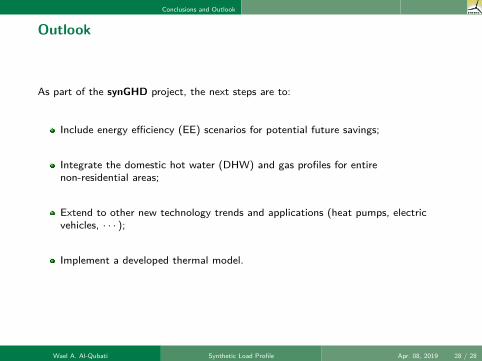
Outlook

As part of the synGHD project, the next steps are to:

Include energy efficiency (EE) scenarios for potential future savings;

Integrate the domestic hot water (DHW) and gas profiles for entirenon-residential areas;

Extend to other new technology trends and applications (heat pumps, electricvehicles, · · · );

Implement a developed thermal model.


References

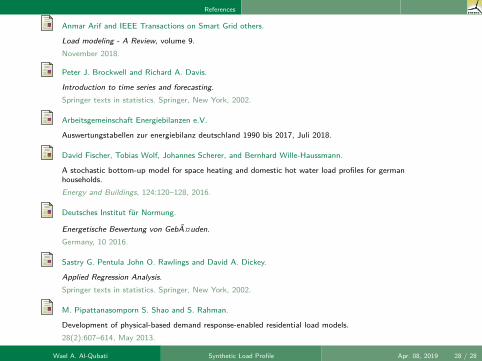
Anmar Arif and IEEE Transactions on Smart Grid others.

Load modeling - A Review, volume 9.November 2018.

Peter J. Brockwell and Richard A. Davis.

Introduction to time series and forecasting.Springer texts in statistics. Springer, New York, 2002.

Arbeitsgemeinschaft Energiebilanzen e.V.

Auswertungstabellen zur energiebilanz deutschland 1990 bis 2017, Juli 2018.

David Fischer, Tobias Wolf, Johannes Scherer, and Bernhard Wille-Haussmann.

A stochastic bottom-up model for space heating and domestic hot water load profiles for germanhouseholds.Energy and Buildings, 124:120–128, 2016.

Deutsches Institut fur Normung.

Energetische Bewertung von GebA¤uden.Germany, 10 2016.

Sastry G. Pentula John O. Rawlings and David A. Dickey.

Applied Regression Analysis.Springer texts in statistics. Springer, New York, 2002.

M. Pipattanasomporn S. Shao and S. Rahman.

Development of physical-based demand response-enabled residential load models.28(2):607–614, May 2013.


References

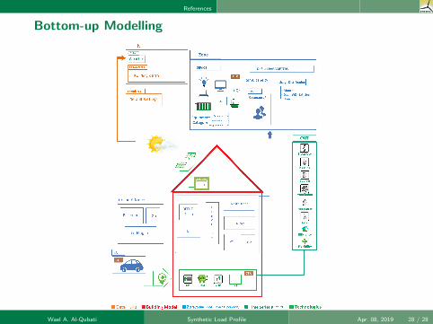
Bottom-up Modelling


References

Box-Jenkins methodology


References

5R1C thermal model of the building


References

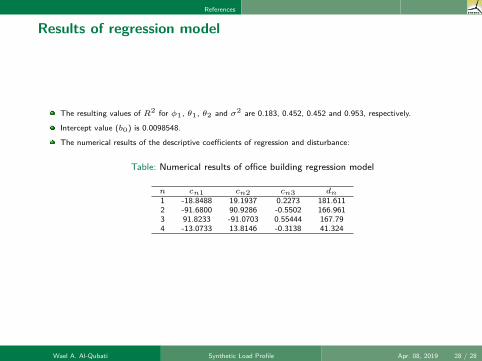
Results of regression model

The resulting values of R2 for φ1, θ1, θ2 and σ2 are 0.183, 0.452, 0.452 and 0.953, respectively.

Intercept value (b0) is 0.0098548.

The numerical results of the descriptive coefficients of regression and disturbance:

Table: Numerical results of office building regression model

n cn1 cn2 cn3 dn

1 -18.8488 19.1937 0.2273 181.6112 -91.6800 90.9286 -0.5502 166.9613 91.8233 -91.0703 0.55444 167.794 -13.0733 13.8146 -0.3138 41.324


Documents

Synthesizing Electrical and Thermal Load Profiles for Non ... · Master Thesis Presentation Wael A. Al-Qubati Renewable Energy and Energy Eﬃciency for the Middle East and North