System Dynamics Shahram Shadrokh -Path Dependence and Positive Feedback -Delay

System Dynamics

Shahram Shadrokh

-Path Dependence and Positive Feedback

-Delay

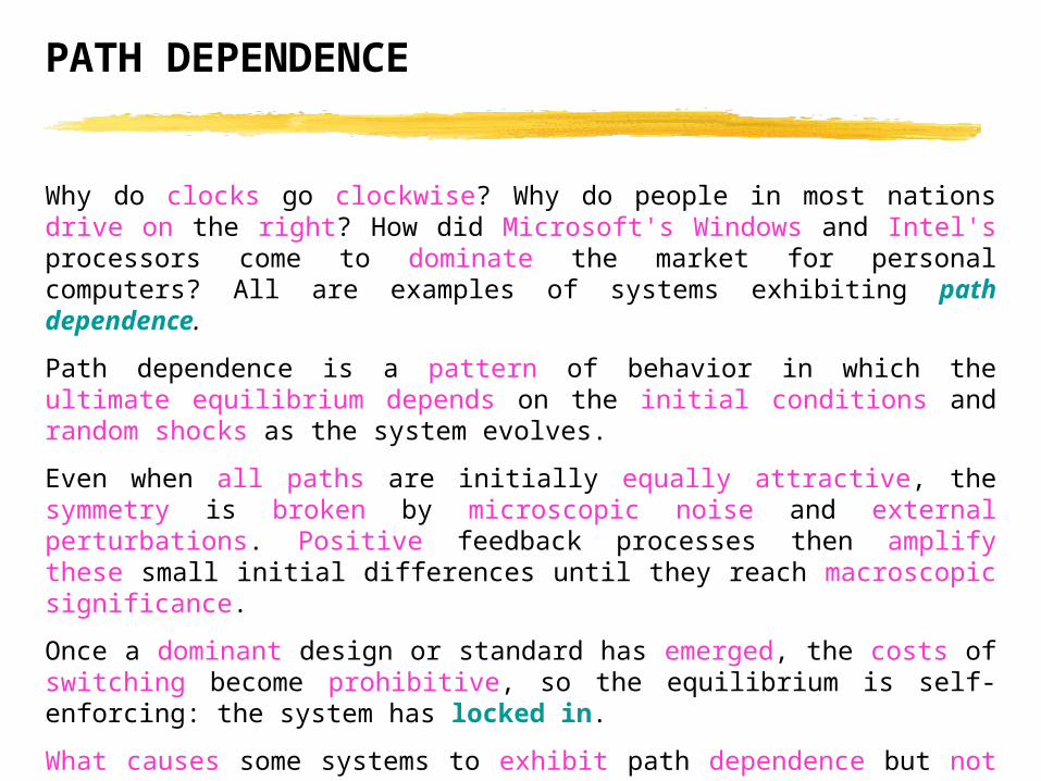
PATH DEPENDENCE

Why do clocks go clockwise? Why do people in most nations drive on the right? How did Microsoft's Windows and Intel's processors come to dominate the market for personal computers? All are examples of systems exhibiting path dependence.

Path dependence is a pattern of behavior in which the ultimate equilibrium depends on the initial conditions and random shocks as the system evolves.

Even when all paths are initially equally attractive, the symmetry is broken by microscopic noise and external perturbations. Positive feedback processes then amplify these small initial differences until they reach macroscopic significance.

Once a dominant design or standard has emerged, the costs of switching become prohibitive, so the equilibrium is self-enforcing: the system has locked in.

What causes some systems to exhibit path dependence but not others? Path dependence arises in systems dominated by positive feedback.

PATH DEPENDENCE

P*

P*

Position ofBall (P)

EquilibriumPosition

(P*)

Discrepancy(P - P*)

Force onBall

+-

-

+

B

Position ofBall (P)

EquilibriumPosition

(P*)

Discrepancy(P - P*)

Force onBall

+-

+

+

R

A SIMPLE MODEL OF PATH DEPENDENCE: THE POLYA PROCESS

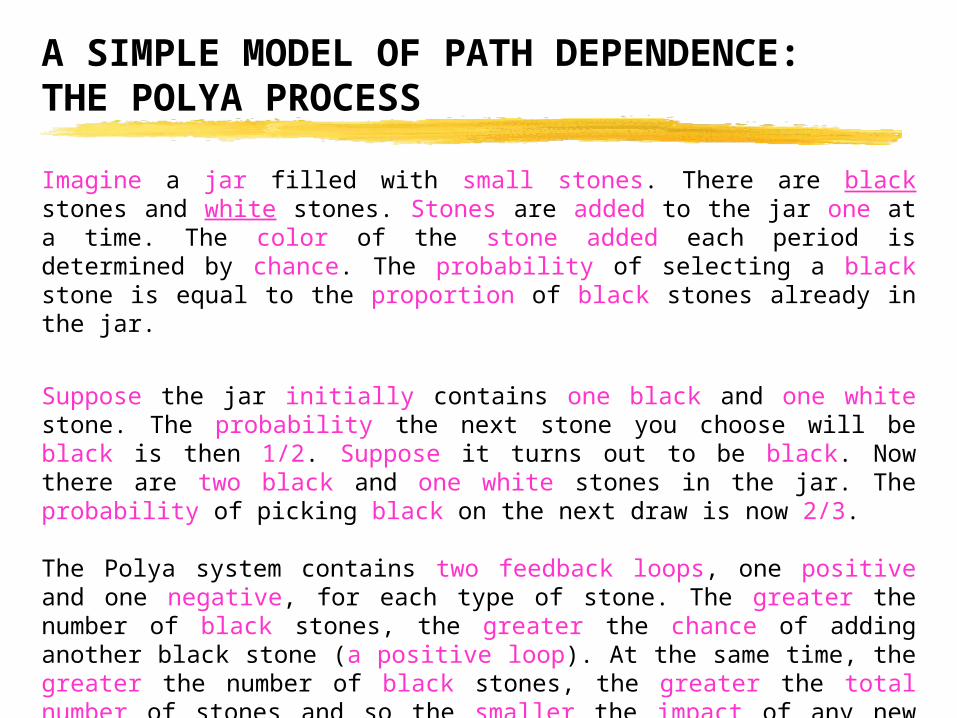
Imagine a jar filled with small stones. There are black stones and white stones. Stones are added to the jar one at a time. The color of the stone added each period is determined by chance. The probability of selecting a black stone is equal to the proportion of black stones already in the jar.

Suppose the jar initially contains one black and one white stone. The probability the next stone you choose will be black is then 1/2. Suppose it turns out to be black. Now there are two black and one white stones in the jar. The probability of picking black on the next draw is now 2/3.

The Polya system contains two feedback loops, one positive and one negative, for each type of stone. The greater the number of black stones, the greater the chance of adding another black stone (a positive loop). At the same time, the greater the number of black stones, the greater the total number of stones and so the smaller the impact of any new black stone added to the jar on the proportion of black stones (a negative loop).

Delay

Modelers need to understand how delays behave, how to represent them, how to choose among various types of delays in any modeling situation, and how to estimate their duration.

A delay is a process whose output lags behind its input in some fashion

There must be at least one stock within every delay. Since the output generally differs from the input (it lags behind), there must be a stock inside the process to accumulate the difference between input and output.

The type of delay shown in figure is known as a material delay, since it captures the physical flow of material (in this case letters) through a delay process.

Many delays represent the gradual adjustment of perceptions or beliefs: these are information delays.

Suppose orders for your product have been steady at 1000 units per day, and you expect them to continue at that rate. Suddenly orders jump to 2000 units/day. You are unlikely to immediately increase your belief about tomorrow's orders to 2000 units. But if the order rate remains at 2000 units/day, day after day, you will gradually increase your expectation of future orders until it eventually reaches the new rate.

MATERIAL DELAYS: STRUCTURE AND BEHAVIOR

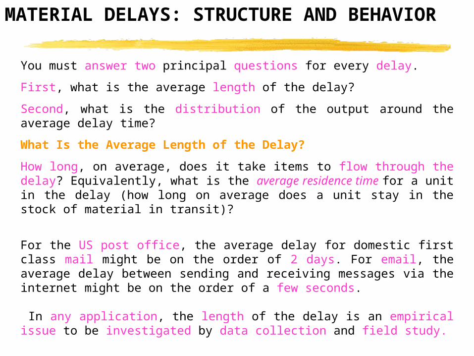
You must answer two principal questions for every delay.

First, what is the average length of the delay?

Second, what is the distribution of the output around the average delay time?

What Is the Average Length of the Delay?

How long, on average, does it take items to flow through the delay? Equivalently, what is the average residence time for a unit in the delay (how long on average does a unit stay in the stock of material in transit)?

For the US post office, the average delay for domestic first class mail might be on the order of 2 days. For email, the average delay between sending and receiving messages via the internet might be on the order of a few seconds.

In any application, the length of the delay is an empirical issue to be investigated by data collection and field study.

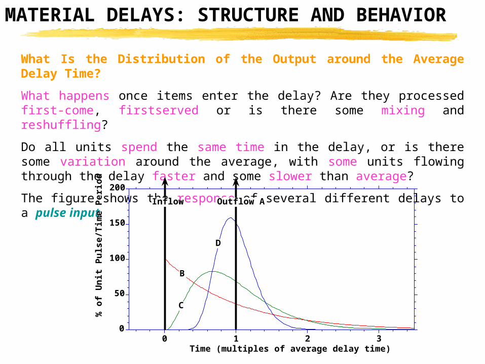
What Is the Distribution of the Output around the Average Delay Time?

What happens once items enter the delay? Are they processed first-come, first served or is there some mixing and reshuffling?

Do all units spend the same time in the delay, or is there some variation around the average, with some units flowing through the delay faster and some slower than average?

The figure shows the response of several different delays to a pulse input.


0

50

100

150

200

0 1 2 3

% o

f U

nit

Pu

lse/

Tim

e P

erio

d

Time (multiples of average delay time)

Inflow

B

C

D

Outflow A

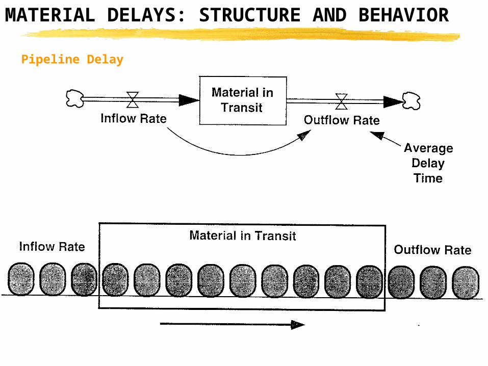
Pipeline Delay

As in the example of the auto assembly line, you sometimes need to model a delay in which the delay time is constant and in which the order of exit from the delay is precisely the same as the order of entry. To do so requires a pipeline delay, also known as transportation lag.

The stock of material in transit for any material delay is given by

Material in Transit = INTEGRAL(Inflow(t) - Outflow(t), Material in Transit(0))

For the pipeline delay, the outflow is simply the inflow lagged by the average delay time D:

Outflow(t) = Inflow(t - D)


First-Order Material Delay

Many delays do not approximate a pipeline 'delay; there is mixing arid variation in the individual processing times, causing some variance in the distribution of deliveries.

Consider an example at the opposite extreme from a pipeline delay, say, water draining from a sink. Further imagine that the water in the sink is thoroughly mixed at all times

In the case of perfect mixing, the probability that any particular water molecule is the next to flow out of the sink is the same for all the molecules in the sink, independent of how long that molecule has been in the sink.

Perfect mixing means the order of entry is irrelevant to the order of exit. Put another way, perfect mixing destroys all information about the order of entry.

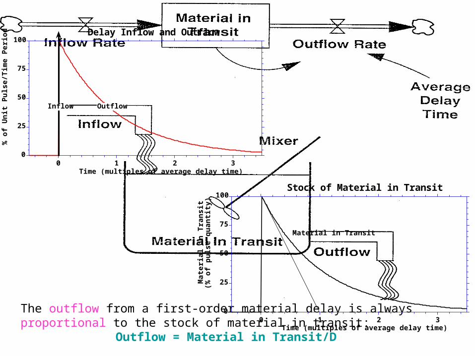
The outflow from a first-order material delay is always proportional to the stock of material in transit:

Outflow = Material in Transit/D


0

25

50

75

100

0 1 2 3

Delay Inflow and Outflow

% o

f U

nit

Pu

lse/

Tim

e P

erio

d


Inflow Outflow

0

25

50

75

100

0 1 2 3

Stock of Material in TransitM

ate

ria

l in

Tra

nsi

t(%

of

pu

lse

qu

an

tity

)


Material in Transit

Higher-Order Material Delays

Between pipeline delay and First-order delay lie many intermediate cases where there is some mixing in the processing order.

In these cases the outflow gradually rises, reaches a peak, and then tails off to zero.

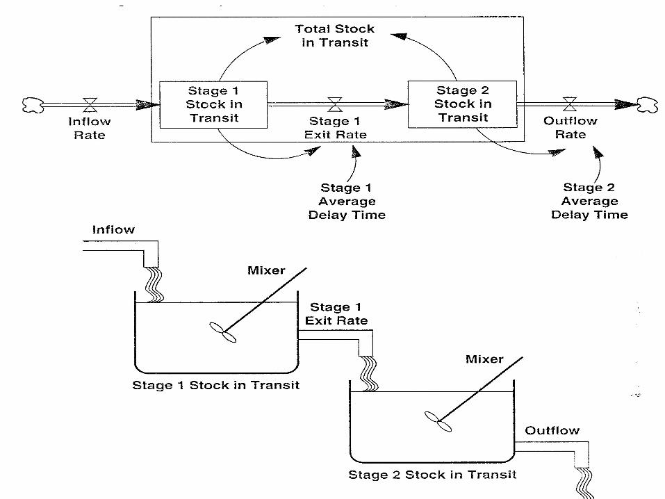
Partial mixing can arise when a delay consists of multiple stages of processing in which items flow sequentially from one stage to the next, but where each stage introduces some mixing.

In many settings the stages of processing in such a system can be approximated well by cascading several first-order material delays together in series. For example, a second-order material delay consists of two first-order delays in which the input to the second stage is the output of the first stage.


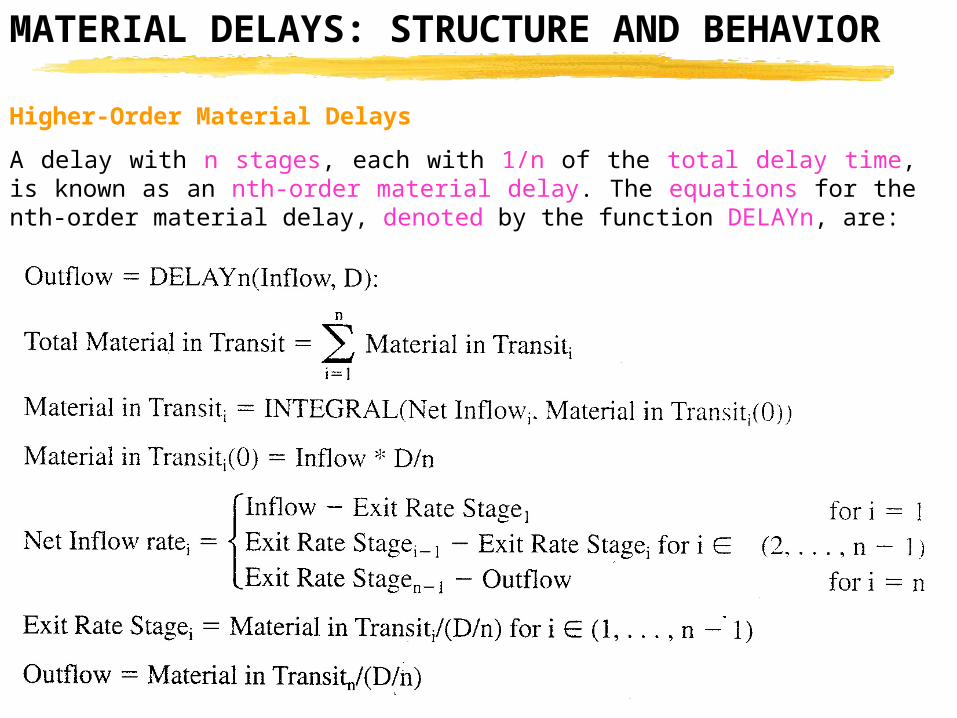
Higher-Order Material Delays

A delay with n stages, each with 1/n of the total delay time, is known as an nth-order material delay. The equations for the nth-order material delay, denoted by the function DELAYn, are:


How Much Is in the Delay? Little's Law

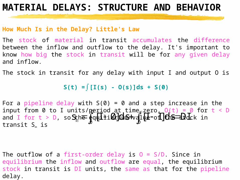
The stock of material in transit accumulates the difference between the inflow and outflow to the delay. It's important to know how big the stock in transit will be for any given delay and inflow.

The stock in transit for any delay with input I and output O is

S(t) =∫[I(s) - O(s)]ds + S(0)

For a pipeline delay with S(0) = 0 and a step increase in the input from 0 to I units/period at time zero, O(t) = 0 for t < D and I for t > D, so the equilibrium value of the stock in transit S∞ is

The outflow of a first-order delay is O = S/D. Since in equilibrium the inflow and outflow are equal, the equilibrium stock in transit is DI units, the same as that for the pipeline delay. In fact, the equilibrium stock in transit for a delay is always DI units, regardless ofthe probability distribution of the outflow. This remarkable property is known as Little's Law


D

0 DDIds]II[ds]0I[s

Many delays exist in channels of information feedback, for example in the measurement or perception of a variable. or in the updating of beliefs and forecasts, such as the perceived order rate for a firm's product or management's belief about future inflation rates.

Why do perceptions and forecasts inevitably involve delays?

All beliefs, expectations, forecasts, and projections are based on information available to the decision maker at the time, which means information about the past.

Information delays cannot be modeled with the same structure used for material delays because there is no physical inflow to a stock of material in transit.

INFORMATION DELAYS: STRUCTURE AND BEHAVIOR

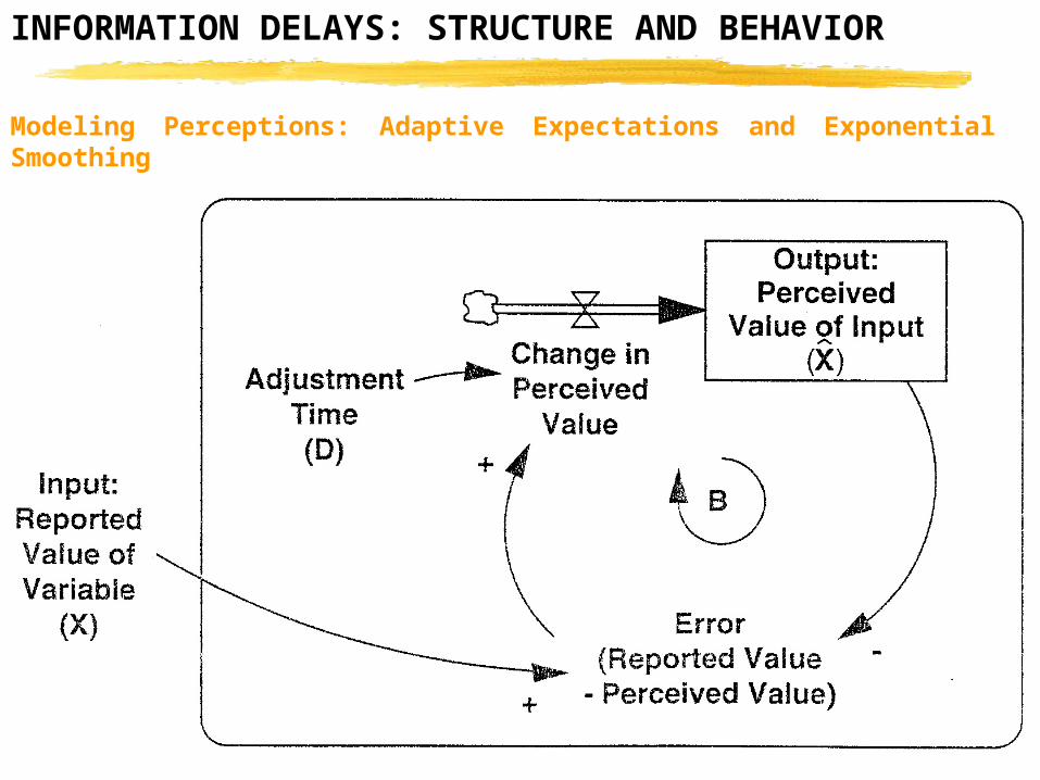
Modeling Perceptions: Adaptive Expectations and Exponential Smoothing

The simplest information delay and one of the most widely used models of beliefadjustment and forecasting is called exponential smoothing or adaptive expectations.

Adaptive expectations mean the belief gradually adjusts to the actual value of the variable. If your belief is persistently wrong, you are likely to revise it until the error is eliminated.

In adaptive expectations the belief or perceived value of the input, X, is a stock:X = INTEGRAL(Change in Perceived Value, X(0))

The rate of change in the belief is proportional to the gap between the current value of the input, X, and the perceived value:

Change in Perceived Value = (X - X)/D


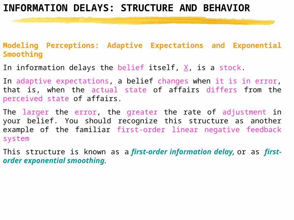
Modeling Perceptions: Adaptive Expectations and Exponential Smoothing

In information delays the belief itself, X, is a stock.

In adaptive expectations, a belief changes when it is in error, that is, when the actual state of affairs differs from the perceived state of affairs.

The larger the error, the greater the rate of adjustment in your belief. You should recognize this structure as another example of the familiar first-order linear negative feedback system

This structure is known as a first-order information delay, or as first-order exponential smoothing.


Higher-Order Information Delays

In a first-order information delay, like the first-order material delay. the output responds immediately to a change in the input. In many cases, however beliefs begin to respond only after some time has passed.

In these cases, the weights on past information are initially low, then build up to a peak before declining.

One way to model a higher-order information delay is with the pipeline delay structure in which the output is simply the input lagged by a constant time period.

Such a delay might be used to model the measurement and reporting processes, where the reported value available to decision makers is the actual value some period of time in the past:

Reported Value(t) = Actual Value (t - D)

More often, the measurement and reporting of information involves multiple stages, and each stage involves some averaging or smoothing.


Higher-Order Information Delays

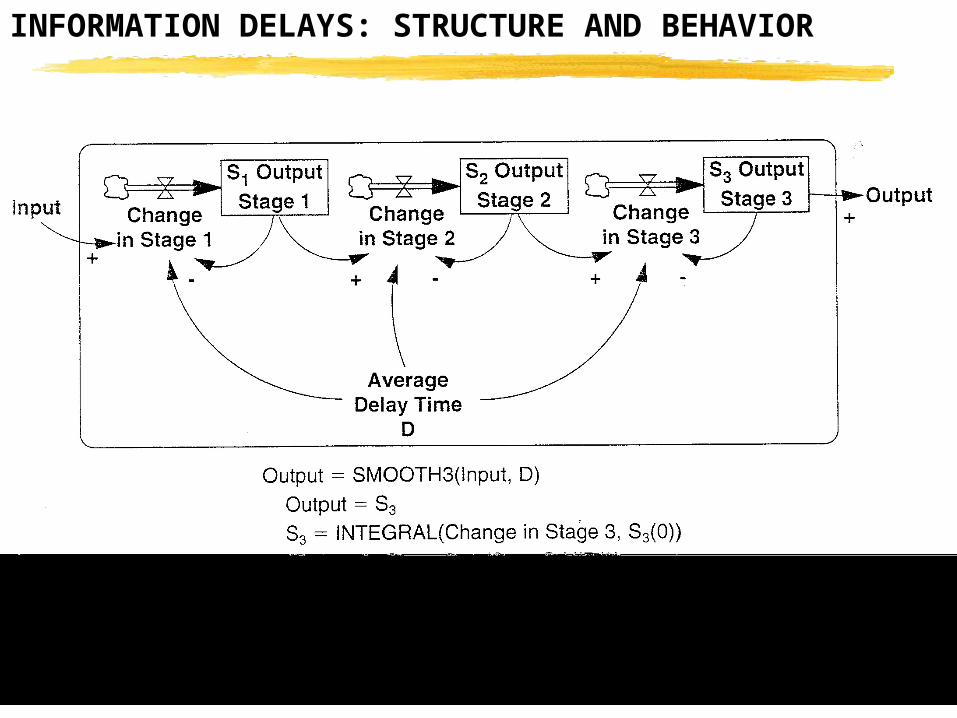
An nth-order information delay, denoted by the SMOOTHn function, consists of n first-order information delays cascaded in series. The perceived value of each stage is the input to the next stage, and the output of the delay is the perceived value of the final stage. Each stage has the same delay time, equal to 1/n of the total delay D:


Documents

System Dynamics Shahram Shadrokh -Path Dependence and Positive Feedback -Delay