Embed Size (px)
Citation preview
System i
Database
DB2 Multisystem
Version 5 Release 4
���

System i
Database
DB2 Multisystem
Version 5 Release 4
���
Note
Before using this information and the product it supports, read the information in “Notices,” on
page 59.
Seventh Edition (February 2006)
This edition applies to version 5, release 4, modification 0 of IBM i5/OS (product number 5722–SS1) and to all
subsequent releases and modifications until otherwise indicated in new editions. This version does not run on all
reduced instruction set computer (RISC) models nor does it run on CISC models.
© Copyright International Business Machines Corporation 1998, 2006. All rights reserved.
US Government Users Restricted Rights – Use, duplication or disclosure restricted by GSA ADP Schedule Contract
with IBM Corp.
Contents
DB2 Multisystem . . . . . . . . . . . 1
What’s new for V5R4 . . . . . . . . . . . 1
Printable PDF . . . . . . . . . . . . . . 1
DB2 Multisystem overview . . . . . . . . . 1
Benefits of using DB2 Multisystem . . . . . . 3
DB2 Multisystem: Basic terms and concepts . . . 3
Node groups with DB2 Multisystem: Overview . . . 5
How node groups work with DB2 Multisystem . . 5
Tasks to complete before using the node group
commands with DB2 Multisystem . . . . . . 6
Create Node Group command . . . . . . . 6
Display Node Group command . . . . . . . 8
Change Node Group Attributes command . . . 10
Delete Node Group command . . . . . . . 11
Distributed files with DB2 Multisystem . . . . . 11
Create Physical File command and SQL CREATE
TABLE statement . . . . . . . . . . . 12
System activities after the distributed file is
created . . . . . . . . . . . . . . . 14
Partitioning with DB2 Multisystem . . . . . 19
Customizing data distribution with DB2
Multisystem . . . . . . . . . . . . . 22
Partitioned tables . . . . . . . . . . . . 22
Creation of partitioned tables . . . . . . . 23
Modification of existing tables . . . . . . . 25
Indexes with partitioned tables . . . . . . . 26
Query performance and optimization . . . . . 27
Save and restore considerations . . . . . . . 31
Journaling a partitioned table . . . . . . . 31
Traditional system interface considerations . . . 31
Restrictions for a partitioned table . . . . . . 32
Scalar functions available with DB2 Multisystem . . 33
PARTITION with DB2 Multisystem . . . . . 33
HASH with DB2 Multisystem . . . . . . . 34
NODENAME with DB2 Multisystem . . . . . 34
NODENUMBER with DB2 Multisystem . . . . 35
Special registers with DB2 Multisystem . . . . 35
Performance and scalability with DB2 Multisystem 36
Why you should use DB2 Multisystem . . . . 36
How DB2 Multisystem helps you expand your
database system . . . . . . . . . . . . 37
Query design for performance with DB2
Multisystem . . . . . . . . . . . . . . 39
Optimization with DB2 Multisystem: Overview 39
Implementation and optimization of a single file
query with DB2 Multisystem . . . . . . . 40
Implementation and optimization of record
ordering with DB2 Multisystem . . . . . . 41
Implementation and optimization of the UNION
and DISTINCT clauses with DB2 Multisystem . . 42
Processing of the DSTDTA and ALWCPYDTA
parameters with DB2 Multisystem . . . . . . 42
Implementation and optimization of join
operations with DB2 Multisystem . . . . . . 42
Implementation and optimization of grouping
with DB2 Multisystem . . . . . . . . . . 47
Subquery support with DB2 Multisystem . . . 49
Access plans with DB2 Multisystem . . . . . 49
Reusable open data paths with DB2 Multisystem 49
Temporary result writer with DB2 Multisystem 51
Optimizer messages with DB2 Multisystem . . . 52
Changes to the Change Query Attributes
command with DB2 Multisystem . . . . . . 54
Summary of performance considerations . . . 55
Related information for DB2 Multisystem . . . . 56
Appendix. Notices . . . . . . . . . . 59
Programming Interface Information . . . . . . 60
Trademarks . . . . . . . . . . . . . . 61
Terms and conditions . . . . . . . . . . . 61
© Copyright IBM Corp. 1998, 2006 iii

iv System i: Database DB2 Multisystem
DB2 Multisystem
Fundamental concepts of DB2® Multisystem include distributed relational database files, node groups,
and partitioning. You can find the information necessary to create and to use database files that are
partitioned across multiple System i™ systems.
Information is provided on how to configure the systems, how to create the files, and how the files can
be used in applications. Table partitioning information is also contained in this topic. Table partitioning
varies from multisystem partitioning in that it is a table partitioned on a single system.
Note: By using the code examples, you agree to the terms of the “Code license and disclaimer
information” on page 57.
What’s new for V5R4
This topic highlights some changes to the DB2 Multisystem for V5R4.
The SQL Query Engine (SQE) provides targeted optimization for partitioned tables using dynamic
partition expansion optimization.
How to see what’s new or changed
To help you see where technical changes have been made, this information uses:
v The
image to mark where new or changed information begins.
v The
image to mark where new or changed information ends.
To find other information about what’s new or changed this release, see the Memo to users.
Printable PDF
Use this to view and print a PDF of this information.
To view or download the PDF version of this document, select DB2 Multisystem (about 869 KB).
Saving PDF files
To save a PDF on your workstation for viewing or printing:
1. Right-click the PDF in your browser (right-click the link above).
2. Click the option that saves the PDF locally.
3. Navigate to the directory in which you want to save the PDF.
4. Click Save.
Downloading Adobe Reader
You need Adobe Reader installed on your system to view or print these PDFs. You can download a free
copy from the Adobe Web site (www.adobe.com/products/acrobat/readstep.html)
.
DB2 Multisystem overview
DB2 Multisystem is a parallel processing technique that provides greater scalability for databases.
© Copyright IBM Corp. 1998, 2006 1
||
|
|
|
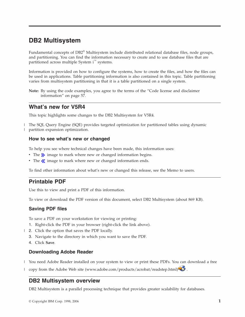
Using DB2 Multisystem, you have the capability to attach multiple System i models (up to 32 systems)
together in a shared-nothing cluster. (Shared-nothing means that each system in the coupled network owns
and manages its own main memory and disk storage.) As soon as the systems are connected, database
files can be spread across the storage units on each connected system. The database files can have data
partitioned (distributed) across a set of systems, and each system has access to all of the data in the file.
Yet to users, the file behaves like a local file on their system. From the user’s perspective, the database
appears as a single database: the user can run queries in parallel across all the systems in the network
and have realtime access to the data in the files.
This parallel processing technique means that heavy use on one system does not degrade the
performance on the other connected systems in the network. If you have large volumes of data and the
need to run queries, DB2 Multisystem provides you with a method of running those queries in one of the
most efficient methods available. In most cases, query performance improves because the queries no
longer run against local files, but run in parallel across several systems.
If you have not yet installed DB2 Multisystem, see Install, upgrade, or delete i5/OS® and related software
for information about installing additional licensed programs. To install DB2 Multisystem, use option 27
in the list of installable options for the operating system.
Figure 1. Distribution of database files across systems
2 System i: Database DB2 Multisystem
Benefits of using DB2 Multisystem
Benefits of using DB2 Multisystem include improved query performance, decreased data replication,
larger database capacity, and so on.
You can realize the benefits of using DB2 Multisystem in several ways:
v Query performance can be improved by running in parallel (pieces of the query are run simultaneously
on different systems).
v The need for data replication decreases because all of the systems can access all of the data.
v Much larger database files can be accommodated.
v Applications are no longer concerned with the location of remote data.
v When growth is needed, you can redistribute the file across more systems, and applications can run
unchanged on the new systems.
With DB2 Multisystem, you can use the same input/output (I/O) methods (GETs, PUTs, and UPDATEs)
or file access methods that you have used in the past. No additional or different I/O methods or file
access methods are required.
Your applications do not need to change; whatever connectivity methods you currently use, unless you
are using OptiConnect, also work for any distributed files you create. With OptiConnect, you must use
the OptiConnect controller descriptions.
Related information
OptiConnect
DB2 Multisystem: Basic terms and concepts
A distributed file is a database file that is spread across multiple System i models. Here are some of the
main concepts regarding the creation and use of distributed files by DB2 Multisystem.
Each system that has a piece of a distributed file is called a node. Each system is identified by the name
that is defined for it in the relational database directory.
A group of systems that contains one or more distributed files is called a node group. A node group is a
system object that contains the list of nodes across which the data is distributed. A system can be a node
in more than one node group.
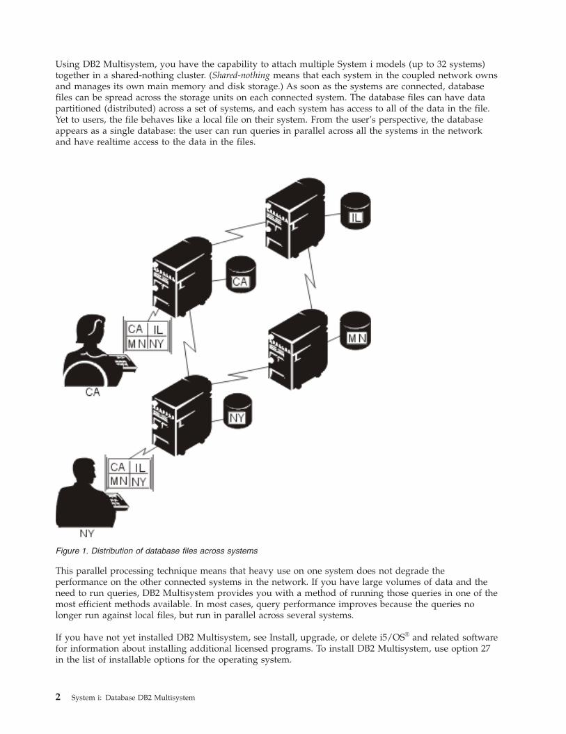
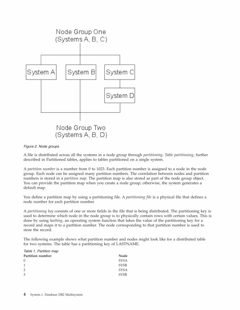
The following figure shows two node groups. Node group one contains systems A, B, and C. Node group
two contains systems A, B, and D. Node groups one and two share systems A and B because a system
can be a node in more than one node group.
DB2 Multisystem 3
A file is distributed across all the systems in a node group through partitioning. Table partitioning, further
described in Partitioned tables, applies to tables partitioned on a single system.
A partition number is a number from 0 to 1023. Each partition number is assigned to a node in the node
group. Each node can be assigned many partition numbers. The correlation between nodes and partition
numbers is stored in a partition map. The partition map is also stored as part of the node group object.
You can provide the partition map when you create a node group; otherwise, the system generates a
default map.
You define a partition map by using a partitioning file. A partitioning file is a physical file that defines a
node number for each partition number.
A partitioning key consists of one or more fields in the file that is being distributed. The partitioning key is
used to determine which node in the node group is to physically contain rows with certain values. This is
done by using hashing, an operating system function that takes the value of the partitioning key for a
record and maps it to a partition number. The node corresponding to that partition number is used to
store the record.
The following example shows what partition number and nodes might look like for a distributed table
for two systems. The table has a partitioning key of LASTNAME.
Table 1. Partition map
Partition number Node
0 SYSA
1 SYSB
2 SYSA
3 SYSB
Figure 2. Node groups
4 System i: Database DB2 Multisystem
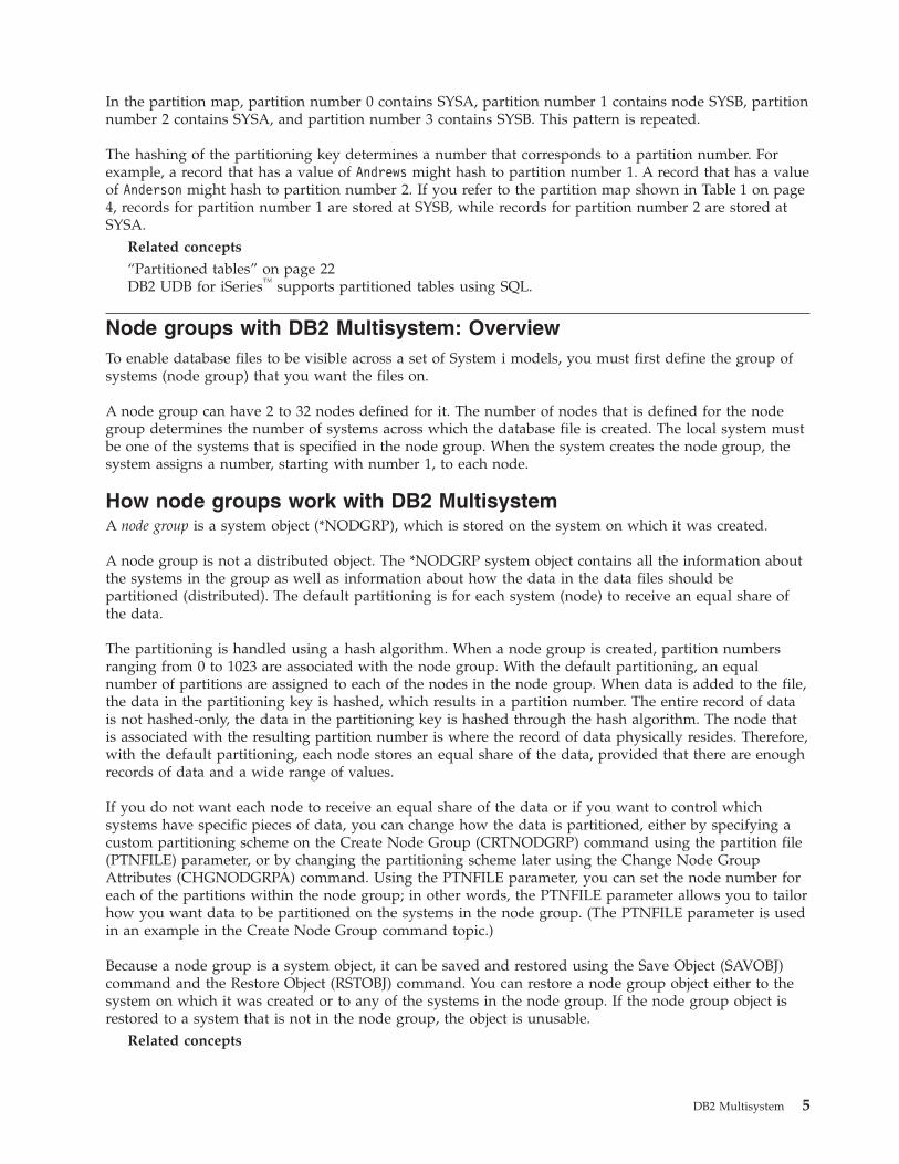
In the partition map, partition number 0 contains SYSA, partition number 1 contains node SYSB, partition
number 2 contains SYSA, and partition number 3 contains SYSB. This pattern is repeated.
The hashing of the partitioning key determines a number that corresponds to a partition number. For
example, a record that has a value of Andrews might hash to partition number 1. A record that has a value
of Anderson might hash to partition number 2. If you refer to the partition map shown in Table 1 on page
4, records for partition number 1 are stored at SYSB, while records for partition number 2 are stored at
SYSA.
Related concepts
“Partitioned tables” on page 22DB2 UDB for iSeries™ supports partitioned tables using SQL.
Node groups with DB2 Multisystem: Overview
To enable database files to be visible across a set of System i models, you must first define the group of
systems (node group) that you want the files on.
A node group can have 2 to 32 nodes defined for it. The number of nodes that is defined for the node
group determines the number of systems across which the database file is created. The local system must
be one of the systems that is specified in the node group. When the system creates the node group, the
system assigns a number, starting with number 1, to each node.
How node groups work with DB2 Multisystem
A node group is a system object (*NODGRP), which is stored on the system on which it was created.
A node group is not a distributed object. The *NODGRP system object contains all the information about
the systems in the group as well as information about how the data in the data files should be
partitioned (distributed). The default partitioning is for each system (node) to receive an equal share of
the data.
The partitioning is handled using a hash algorithm. When a node group is created, partition numbers
ranging from 0 to 1023 are associated with the node group. With the default partitioning, an equal
number of partitions are assigned to each of the nodes in the node group. When data is added to the file,
the data in the partitioning key is hashed, which results in a partition number. The entire record of data
is not hashed-only, the data in the partitioning key is hashed through the hash algorithm. The node that
is associated with the resulting partition number is where the record of data physically resides. Therefore,
with the default partitioning, each node stores an equal share of the data, provided that there are enough
records of data and a wide range of values.
If you do not want each node to receive an equal share of the data or if you want to control which
systems have specific pieces of data, you can change how the data is partitioned, either by specifying a
custom partitioning scheme on the Create Node Group (CRTNODGRP) command using the partition file
(PTNFILE) parameter, or by changing the partitioning scheme later using the Change Node Group
Attributes (CHGNODGRPA) command. Using the PTNFILE parameter, you can set the node number for
each of the partitions within the node group; in other words, the PTNFILE parameter allows you to tailor
how you want data to be partitioned on the systems in the node group. (The PTNFILE parameter is used
in an example in the Create Node Group command topic.)
Because a node group is a system object, it can be saved and restored using the Save Object (SAVOBJ)
command and the Restore Object (RSTOBJ) command. You can restore a node group object either to the
system on which it was created or to any of the systems in the node group. If the node group object is
restored to a system that is not in the node group, the object is unusable.
Related concepts
DB2 Multisystem 5
“Create Node Group command”Two CL command examples show you how to create a node group by using the Create Node Group
(CRTNODGRP) command.
“Partitioning with DB2 Multisystem” on page 19Partitioning is the process of distributing a file across the nodes in a node group.
Tasks to complete before using the node group commands with DB2
Multisystem
Before using the Create Node Group (CRTNODGRP) command or any of the node group commands, you
must ensure that the distributed relational database network you are using has been properly set up.
If this is a new distributed relational database network, you can use the distributed database
programming information to help establish the network.
You need to ensure that one system in the network is defined as the local (*LOCAL) system. Use the
Work with RDB (Relational Database) Directory Entries (WRKRDBDIRE) command to display the details
about the entries. If a local system is not defined, you can do so by specifying *LOCAL for the remote
location name (RMTLOCNAME) parameter of the Add RDB Directory Entries (ADDRDBDIRE)
command, for example:
ADDRDBDIRE RDB(MP000) RMTLOCNAME(*LOCAL) TEXT (’New York’)
The system in New York, named MP000, is defined as the local system in the relational database
directory. You can define only one local relational database as the system name or local location name for
the system in your network configuration. This can help you identify a database name and correlate it to
a particular system in your distributed relational database network, especially if your network is
complex.
For DB2 Multisystem to properly distribute files to the systems within the node groups that you define,
you must have the remote database (RDB) names consistent across all the nodes (systems) in the node
group.
For example, if you plan to have three systems in your node group, each system must have at least three
entries in the RDB directory. On each system, the three names must all be the same. On each of the three
systems, an entry exists for the local system, which is identified as *LOCAL. The other two entries
contain the appropriate remote location information.
Related concepts
Distributed database programming
Create Node Group command
Two CL command examples show you how to create a node group by using the Create Node Group
(CRTNODGRP) command.
In the following example, a node group with default partitioning (equal partitioning across the systems)
is created:
CRTNODGRP NODGRP(LIB1/GROUP1) RDB(SYSTEMA SYSTEMB SYSTEMC SYSTEMD)
TEXT(’Node group for test files’)
In this example, the command creates a node group that contains four nodes. Note that each of the nodes
must be defined RDB entries (previously added to the relational database directory using the
ADDRDBDIRE command) and that one node must be defined as local (*LOCAL).
The partitioning attributes default to assigning one-fourth of the partitions to each node number. This
node group can be used on the NODGRP parameter of the Create Physical File (CRTPF) command to
create a distributed file.
6 System i: Database DB2 Multisystem
In the following example, a node group with specified partitioning is created by using the partitioning
file (PTNFILE) parameter:
CRTNODGRP NODGRP(LIB1/GROUP2) RDB(SYSTEMA SYSTEMB SYSTEMC)
PTNFILE(LIB1/PTN1)
TEXT(’Partition most of the data to SYSTEMA’)
In this example, the command creates a node group that contains three nodes (SYSTEMA, SYSTEMB, and
SYSTEMC). The partitioning attributes are taken from the file called PTN1. This file can be set up to force
a higher percentage of the records to be located on a particular system.
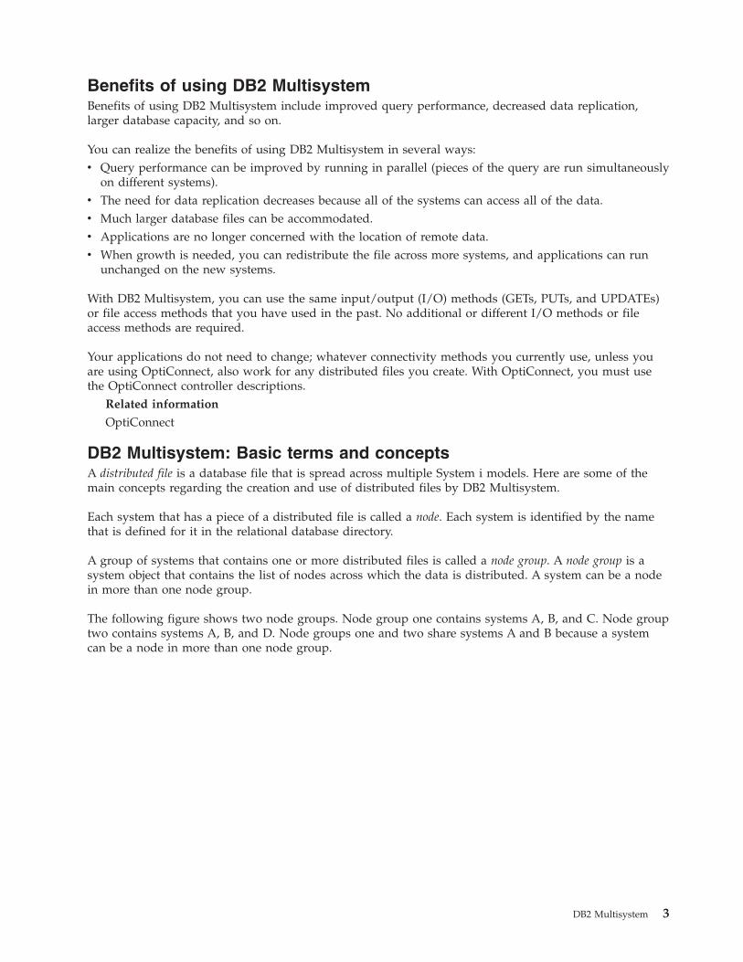
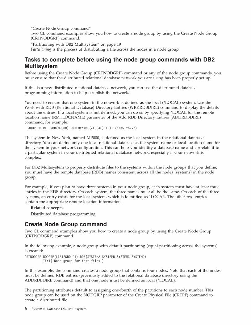
The file PTN1 in this example is a partitioning file. This file is not a distributed file, but a regular local
physical file that can be used to set up a custom partitioning scheme. The partitioning file must have one
2-byte binary field. The partitioning file must contain 1024 records in which each record contains a valid
node number.
If the node group contains three nodes, all of the records in the partitioning file must have numbers 1, 2,
or 3. The node numbers are assigned in the order that the RDB names were specified on the Create Node
Group (CRTNODGRP) command. A higher percentage of data can be forced to a particular node by
having more records containing that node number in the partitioning file. This is a method for
customizing the partitioning with respect to the amount of data that physically resides on each system.
To customize the partitioning with respect to specific values residing on specific nodes, use the Change
Node Group Attributes (CHGNODGRPA) command.
You should note that, because the node group information is stored in the distributed file, the file is not
immediately sensitive to changes in the node group or to changes in the RDB directory entries that are
included in the node group. You can make modifications to node groups and RDB directory entries, but
until you use the CHGPF command and specify the changed node group, your files do not change their
behavior.
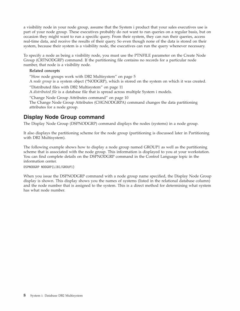
Another concept is that of a visibility node. A visibility node within a node group contains the file object
(part of the mechanism that allows the file to be distributed across several nodes), but no data. A
visibility node retains a current level of the file object at all times; the visibility node has no data stored
on it. In contrast, a node (sometimes called a data node) contains data. As an example of how you can use
Figure 3. Example of the contents of partitioning file PTNFILE
DB2 Multisystem 7
a visibility node in your node group, assume that the System i product that your sales executives use is
part of your node group. These executives probably do not want to run queries on a regular basis, but on
occasion they might want to run a specific query. From their system, they can run their queries, access
real-time data, and receive the results of their query. So even though none of the data is stored on their
system, because their system is a visibility node, the executives can run the query whenever necessary.
To specify a node as being a visibility node, you must use the PTNFILE parameter on the Create Node
Group (CRTNODGRP) command. If the partitioning file contains no records for a particular node
number, that node is a visibility node.
Related concepts
“How node groups work with DB2 Multisystem” on page 5A node group is a system object (*NODGRP), which is stored on the system on which it was created.
“Distributed files with DB2 Multisystem” on page 11A distributed file is a database file that is spread across multiple System i models.
“Change Node Group Attributes command” on page 10The Change Node Group Attributes (CHGNODGRPA) command changes the data partitioning
attributes for a node group.
Display Node Group command
The Display Node Group (DSPNODGRP) command displays the nodes (systems) in a node group.
It also displays the partitioning scheme for the node group (partitioning is discussed later in Partitioning
with DB2 Multisystem).
The following example shows how to display a node group named GROUP1 as well as the partitioning
scheme that is associated with the node group. This information is displayed to you at your workstation.
You can find complete details on the DSPNODGRP command in the Control Language topic in the
information center.
DSPNODGRP NODGRP(LIB1/GROUP1)
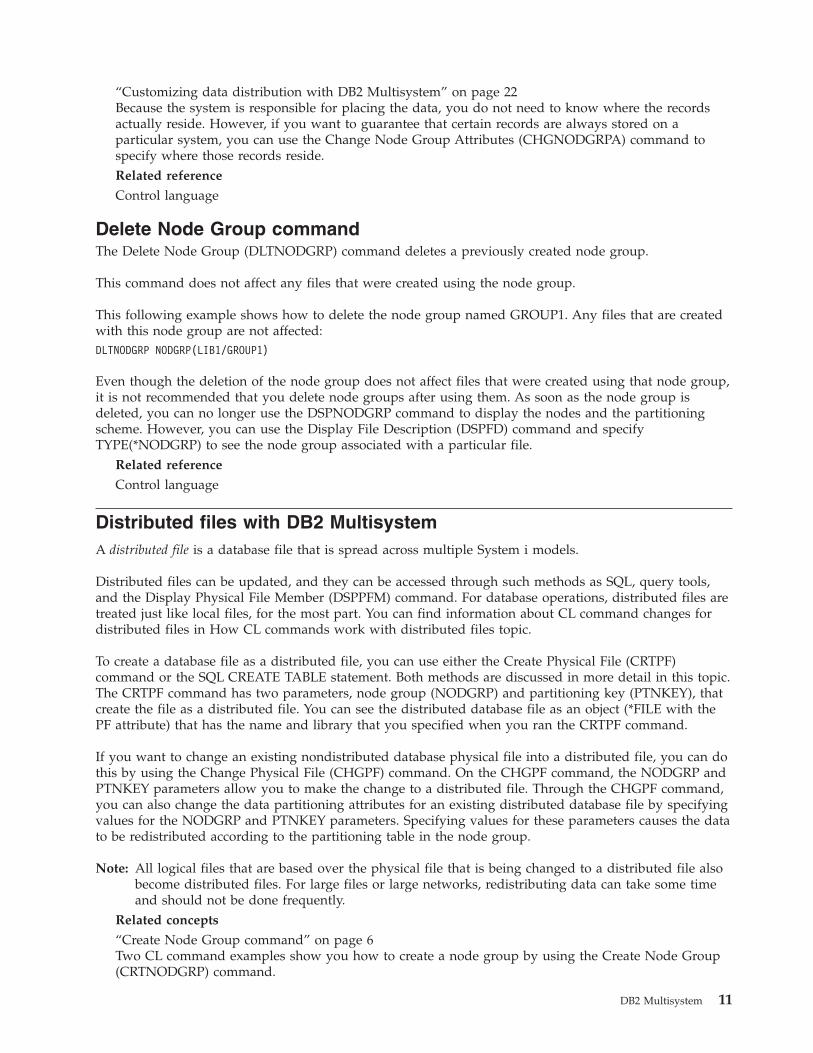
When you issue the DSPNODGRP command with a node group name specified, the Display Node Group
display is shown. This display shows you the names of systems (listed in the relational database column)
and the node number that is assigned to the system. This is a direct method for determining what system
has what node number.
8 System i: Database DB2 Multisystem
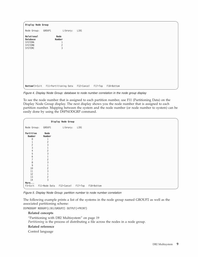
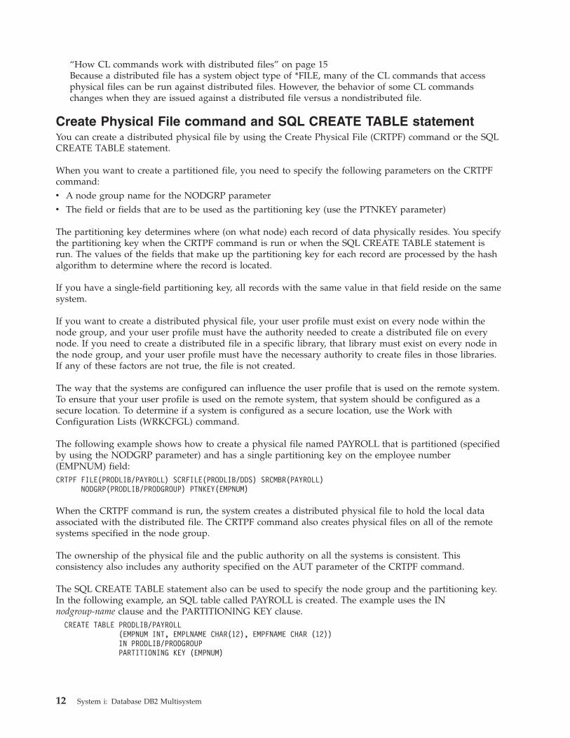
To see the node number that is assigned to each partition number, use F11 (Partitioning Data) on the
Display Node Group display. The next display shows you the node number that is assigned to each
partition number. Mapping between the system and the node number (or node number to system) can be
easily done by using the DSPNODGRP command.
The following example prints a list of the systems in the node group named GROUP2 as well as the
associated partitioning scheme:
DSPNODGRP NODGRP(LIB1/GROUP2) OUTPUT(*PRINT)
Related concepts
“Partitioning with DB2 Multisystem” on page 19Partitioning is the process of distributing a file across the nodes in a node group.
Related reference
Control language
Display Node Group
Node Group: GROUP1 Library: LIB1
Relational Node
Database Number
SYSTEMA 1
SYSTEMB 2
SYSTEMC 3
BottomF3=Exit F11=Partitioning Data F12=Cancel F17=Top F18=Bottom
Figure 4. Display Node Group: database to node number correlation in the node group display
Display Node Group
Node Group: GROUP1 Library: LIB1
Partition Node
Number Number
0 1
1 2
2 3
3 1
4 2
5 3
6 1
7 2
8 3
9 1
10 2
11 3
12 1
13 2
14 3
More...
F3=Exit F11=Node Data F12=Cancel F17=Top F18=Bottom
Figure 5. Display Node Group: partition number to node number correlation
DB2 Multisystem 9

Change Node Group Attributes command
The Change Node Group Attributes (CHGNODGRPA) command changes the data partitioning attributes
for a node group.
The node group contains a table with 1024 partitions; each partition contains a node number. Node
numbers were assigned when the node group was created and correspond to the relational databases
specified on the RDB parameter of the Create Node Group (CRTNODGRP) command. Use the Display
Node Group (DSPNODGRP) command to see the valid node number values and the correlation between
node numbers and relational database names.
The CHGNODGRPA command does not affect any existing distributed files that were created using the
specified node group. For the changed node group to be used, the changed node group must be specified
either when creating a new file or on the Change Physical File (CHGPF) command. You can find
complete details on the CHGNODGRPA command in the Control Language topic in the Information
Center.
This first example shows how to change the partitioning attributes of the node group named GROUP1 in
library LIB1:
CHGNODGRPA NODGRP(LIB1/GROUP1) PTNNBR(1019)
NODNBR(2)
In this example, the partition number 1019 is specified, and any records that hash to 1019 are written to
node number 2. This provides a method for directing specific partition numbers to specific nodes within
a node group.
The second example changes the partitioning attributes of the node group named GROUP2. (GROUP2 is
found by using the library search list, *LIBL.) The value specified on the comparison data value
(CMPDTA) parameter is hashed, and the resulting partition number is changed from its existing node
number to node number 3. (Hashing and partitioning are discussed in Partitioning with DB2
Multisystem.)
CHGNODGRPA NODGRP(GROUP2) CMPDTA(’CHICAGO’)
NODNBR(3)
Any files that are created using this node group and that have a partitioning key consisting of a character
field store records that contain ’CHICAGO’ in the partitioning key on node number 3. To allow for files
with multiple fields in the partitioning key, you can specify up to 300 values on the compare data
(CMPDTA) parameter.
When you enter values on the CMPDTA parameter, you should be aware that the character data is
case-sensitive. This means that ’Chicago’ and ’CHICAGO’ do not result in the same partition number.
Numeric data should be entered only as numeric digits; do not use a decimal point, leading zeros, or
following zeros.
All values are hashed to obtain a partition number, which is then associated with the node number that is
specified on the node number (NODNBR) parameter. The text of the completion message, CPC3207,
shows the partition number that was changed. Be aware that by issuing the CHGNODGRPA command
many times and for many different values that you increase the chance of changing the same partition
number twice. If this occurs, the node number that is specified on the most recent change is in effect for
the node group.
Related concepts
“Create Node Group command” on page 6Two CL command examples show you how to create a node group by using the Create Node Group
(CRTNODGRP) command.
“Partitioning with DB2 Multisystem” on page 19Partitioning is the process of distributing a file across the nodes in a node group.
10 System i: Database DB2 Multisystem
“Customizing data distribution with DB2 Multisystem” on page 22Because the system is responsible for placing the data, you do not need to know where the records
actually reside. However, if you want to guarantee that certain records are always stored on a
particular system, you can use the Change Node Group Attributes (CHGNODGRPA) command to
specify where those records reside. Related reference
Control language
Delete Node Group command
The Delete Node Group (DLTNODGRP) command deletes a previously created node group.
This command does not affect any files that were created using the node group.
This following example shows how to delete the node group named GROUP1. Any files that are created
with this node group are not affected:
DLTNODGRP NODGRP(LIB1/GROUP1)
Even though the deletion of the node group does not affect files that were created using that node group,
it is not recommended that you delete node groups after using them. As soon as the node group is
deleted, you can no longer use the DSPNODGRP command to display the nodes and the partitioning
scheme. However, you can use the Display File Description (DSPFD) command and specify
TYPE(*NODGRP) to see the node group associated with a particular file.
Related reference
Control language
Distributed files with DB2 Multisystem
A distributed file is a database file that is spread across multiple System i models.
Distributed files can be updated, and they can be accessed through such methods as SQL, query tools,
and the Display Physical File Member (DSPPFM) command. For database operations, distributed files are
treated just like local files, for the most part. You can find information about CL command changes for
distributed files in How CL commands work with distributed files topic.
To create a database file as a distributed file, you can use either the Create Physical File (CRTPF)
command or the SQL CREATE TABLE statement. Both methods are discussed in more detail in this topic.
The CRTPF command has two parameters, node group (NODGRP) and partitioning key (PTNKEY), that
create the file as a distributed file. You can see the distributed database file as an object (*FILE with the
PF attribute) that has the name and library that you specified when you ran the CRTPF command.
If you want to change an existing nondistributed database physical file into a distributed file, you can do
this by using the Change Physical File (CHGPF) command. On the CHGPF command, the NODGRP and
PTNKEY parameters allow you to make the change to a distributed file. Through the CHGPF command,
you can also change the data partitioning attributes for an existing distributed database file by specifying
values for the NODGRP and PTNKEY parameters. Specifying values for these parameters causes the data
to be redistributed according to the partitioning table in the node group.
Note: All logical files that are based over the physical file that is being changed to a distributed file also
become distributed files. For large files or large networks, redistributing data can take some time
and should not be done frequently.
Related concepts
“Create Node Group command” on page 6Two CL command examples show you how to create a node group by using the Create Node Group
(CRTNODGRP) command.
DB2 Multisystem 11
“How CL commands work with distributed files” on page 15Because a distributed file has a system object type of *FILE, many of the CL commands that access
physical files can be run against distributed files. However, the behavior of some CL commands
changes when they are issued against a distributed file versus a nondistributed file.
Create Physical File command and SQL CREATE TABLE statement
You can create a distributed physical file by using the Create Physical File (CRTPF) command or the SQL
CREATE TABLE statement.
When you want to create a partitioned file, you need to specify the following parameters on the CRTPF
command:
v A node group name for the NODGRP parameter
v The field or fields that are to be used as the partitioning key (use the PTNKEY parameter)
The partitioning key determines where (on what node) each record of data physically resides. You specify
the partitioning key when the CRTPF command is run or when the SQL CREATE TABLE statement is
run. The values of the fields that make up the partitioning key for each record are processed by the hash
algorithm to determine where the record is located.
If you have a single-field partitioning key, all records with the same value in that field reside on the same
system.
If you want to create a distributed physical file, your user profile must exist on every node within the
node group, and your user profile must have the authority needed to create a distributed file on every
node. If you need to create a distributed file in a specific library, that library must exist on every node in
the node group, and your user profile must have the necessary authority to create files in those libraries.
If any of these factors are not true, the file is not created.
The way that the systems are configured can influence the user profile that is used on the remote system.
To ensure that your user profile is used on the remote system, that system should be configured as a
secure location. To determine if a system is configured as a secure location, use the Work with
Configuration Lists (WRKCFGL) command.
The following example shows how to create a physical file named PAYROLL that is partitioned (specified
by using the NODGRP parameter) and has a single partitioning key on the employee number
(EMPNUM) field:
CRTPF FILE(PRODLIB/PAYROLL) SCRFILE(PRODLIB/DDS) SRCMBR(PAYROLL)
NODGRP(PRODLIB/PRODGROUP) PTNKEY(EMPNUM)
When the CRTPF command is run, the system creates a distributed physical file to hold the local data
associated with the distributed file. The CRTPF command also creates physical files on all of the remote
systems specified in the node group.
The ownership of the physical file and the public authority on all the systems is consistent. This
consistency also includes any authority specified on the AUT parameter of the CRTPF command.
The SQL CREATE TABLE statement also can be used to specify the node group and the partitioning key.
In the following example, an SQL table called PAYROLL is created. The example uses the IN
nodgroup-name clause and the PARTITIONING KEY clause.
CREATE TABLE PRODLIB/PAYROLL
(EMPNUM INT, EMPLNAME CHAR(12), EMPFNAME CHAR (12))
IN PRODLIB/PRODGROUP
PARTITIONING KEY (EMPNUM)
12 System i: Database DB2 Multisystem
When the PARTITIONING KEY clause is not specified, the first column of the primary key, if one is
defined, is used as the first partitioning key. If no primary key is defined, the first column defined for the
table that does not have a data type of date, time, timestamp, or floating-point numeric is used as the
partitioning key.
To see if a file is partitioned, use the Display File Description (DSPFD) command. If the file is partitioned,
the DSPFD command shows the name of the node group, shows the details of the node group stored in
the file object (including the entire partition map), and lists the fields of the partitioning key.
You can find a list of restrictions you need to know when using distributed files with DB2 Multisystem in
the Restrictions when creating or working with distributed files with DB2 Multisystem topic.
Related concepts
Distributed database programming
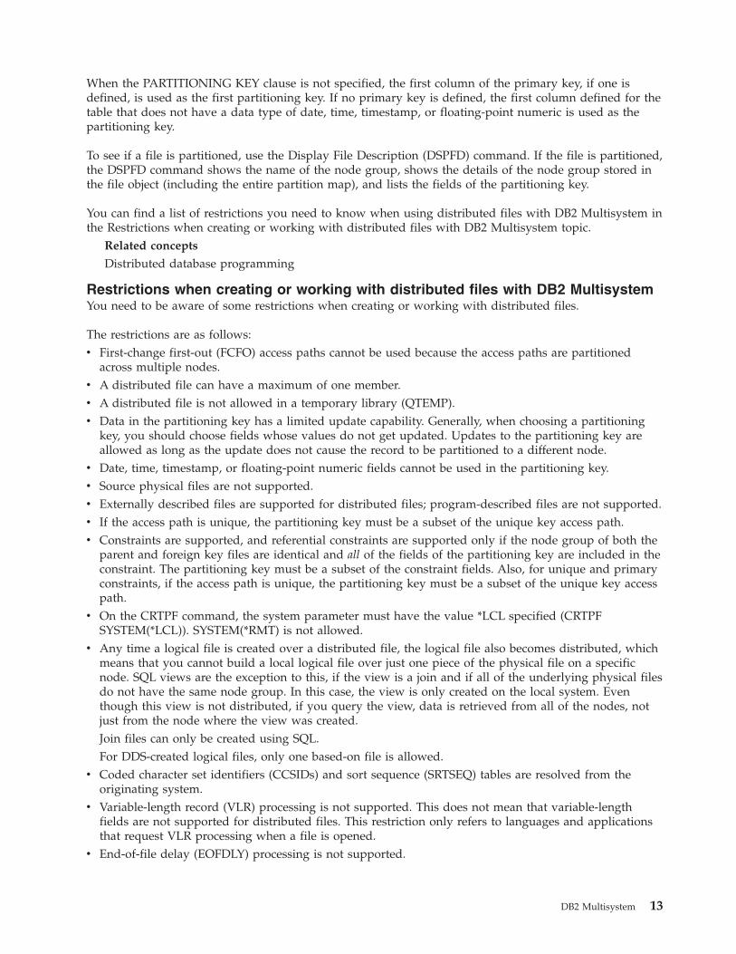
Restrictions when creating or working with distributed files with DB2 Multisystem
You need to be aware of some restrictions when creating or working with distributed files.
The restrictions are as follows:
v First-change first-out (FCFO) access paths cannot be used because the access paths are partitioned
across multiple nodes.
v A distributed file can have a maximum of one member.
v A distributed file is not allowed in a temporary library (QTEMP).
v Data in the partitioning key has a limited update capability. Generally, when choosing a partitioning
key, you should choose fields whose values do not get updated. Updates to the partitioning key are
allowed as long as the update does not cause the record to be partitioned to a different node.
v Date, time, timestamp, or floating-point numeric fields cannot be used in the partitioning key.
v Source physical files are not supported.
v Externally described files are supported for distributed files; program-described files are not supported.
v If the access path is unique, the partitioning key must be a subset of the unique key access path.
v Constraints are supported, and referential constraints are supported only if the node group of both the
parent and foreign key files are identical and all of the fields of the partitioning key are included in the
constraint. The partitioning key must be a subset of the constraint fields. Also, for unique and primary
constraints, if the access path is unique, the partitioning key must be a subset of the unique key access
path.
v On the CRTPF command, the system parameter must have the value *LCL specified (CRTPF
SYSTEM(*LCL)). SYSTEM(*RMT) is not allowed.
v Any time a logical file is created over a distributed file, the logical file also becomes distributed, which
means that you cannot build a local logical file over just one piece of the physical file on a specific
node. SQL views are the exception to this, if the view is a join and if all of the underlying physical files
do not have the same node group. In this case, the view is only created on the local system. Even
though this view is not distributed, if you query the view, data is retrieved from all of the nodes, not
just from the node where the view was created.
Join files can only be created using SQL.
For DDS-created logical files, only one based-on file is allowed.
v Coded character set identifiers (CCSIDs) and sort sequence (SRTSEQ) tables are resolved from the
originating system.
v Variable-length record (VLR) processing is not supported. This does not mean that variable-length
fields are not supported for distributed files. This restriction only refers to languages and applications
that request VLR processing when a file is opened.
v End-of-file delay (EOFDLY) processing is not supported.
DB2 Multisystem 13
v Data File Utility (DFU) does not work against distributed files, because DFU uses relative record
number processing to access records.
v A distributed file cannot be created into a library located on an independent auxiliary storage pool
(IASP).
System activities after the distributed file is created
As soon as the file is created, the system ensures that the data is partitioned and that the files remain at
concurrent levels.
As soon as the file is created, the following activities occur automatically:
v All indexes created for the file are created on all the nodes.
v Authority chaninformation about using distributed files with DB2 Multisystemges are sent to all nodes.
v The system prevents the file from being moved and prevents its library from being renamed.
v If the file itself is renamed, its new name is reflected on all nodes.
v Several commands, such as Allocate Object (ALCOBJ), Reorganize Physical File Member (RGZPFM),
and Start Journal Physical File (STRJRNPF), now affect all of the pieces of the file. This allows you to
maintain the concept of a local file when working with partitioned files. See CL commands: Affecting
all the pieces of a distributed file with DB2 Multisystem for a complete list of these CL commands.
You can issue the Allocate Object (ALCOBJ) command from any of the nodes in the node group. This
locks all the pieces and ensures the same integrity that is granted when a local file is allocated. All of
these actions are handled by the system, which keeps you from having to enter the commands on each
node.
In the case of the Start Journal Physical File (STRJRNPF) command, journaling is started on each
system. Therefore, each system must have its own journal and journal receiver. Each system has its
own journal entries; recovery using the journal entries must be done on each system individually. The
commands to start and end journaling affect all of the systems in the node group simultaneously.
v Several commands, such as Dump Object (DMPOBJ), Save Object (SAVOBJ), and Work with Object
Locks (WRKOBJLCK), only affect the piece of the file on the system where the command was issued.
See CL Commands: Affecting only local pieces of a distributed file with DB2 Multisystem for a
complete list of these CL commands.
As soon as a file is created as a distributed file, the opening of the file results in an opening of the local
piece of the file as well as connections being made to all of the remote systems. When the file is created,
it can be accessed from any of the systems in the node group. The system also determines which nodes
and records it needs to use to complete the file I/O task (GETS, PUTs, and UPDATES, for example). You
do not need to physically influence or specify any of this activity.
Note that Distributed Relational Database Architecture™ (DRDA®) and distributed data management
(DDM) requests can target distributed files. Previously distributed applications that use DRDA or DDM
to access a database file on a remote system can continue to work even if that database file was changed
to be a distributed file.
You should be aware that the arrival sequence of the records is different for distributed database files
than that of a local database file.
Because distributed files are physically distributed across systems, you cannot rely on the arrival
sequence or relative record number of the records. With a local database file, the records are dealt with in
order. If, for example, you are inserting data into a local database file, the data is inserted starting with
the first record and continuing through the last record. All records are inserted in sequential order.
Records on an individual node are inserted the same way that records are inserted for a local file.
When data is read from a local database file, the data is read from the first record on through the last
record. This is not true for a distributed database file. With a distributed database file, the data is read
14 System i: Database DB2 Multisystem
from the records (first to last record) in the first node, then the second node, and so on. For example,
reading to record 27 no longer means that you read to a single record. With a distributed file, each node
in the node group can contain its own record 27, none of which is the same.
Related concepts
“CL commands: Affecting all the pieces of a distributed file with DB2 Multisystem” on page 16Some CL commands, when run, affect all the pieces of the distributed file.
“Journaling considerations with DB2 Multisystem” on page 18Although the Start Journal Physical File (STRJRNPF) and End Journal Physical File (ENDJRNPF)
commands are distributed to other systems, the actual journaling takes place on each system
independently and to each system’s own journal receiver.
“CL commands: Affecting only local pieces of a distributed file with DB2 Multisystem”Some CL commands, when run, affect only the piece of the distributed file that is located on the local
system (the system from which the command is run).
How CL commands work with distributed files
Because a distributed file has a system object type of *FILE, many of the CL commands that access
physical files can be run against distributed files. However, the behavior of some CL commands changes
when they are issued against a distributed file versus a nondistributed file.
Related concepts
“Distributed files with DB2 Multisystem” on page 11A distributed file is a database file that is spread across multiple System i models.
Related reference
Control language
CL commands: Allowable to run against a distributed file with DB2 Multisystem:
Some CL commands or specific parameters cannot be run against distributed files.
These CL commands or parameters are as follows:
v SHARE parameter of the Change Logical File Member (CHGLFM)
v SHARE parameter of the Change Physical File Member (CHGPFM)
v Create Duplicate Object (CRTDUPOBJ)
v Initialize Physical File Member (INZPFM)
v Move Object (MOVOBJ)
v Position Database File (POSDBF)
v Remove Member (RMVM)
v Rename Library (RNMLIB) for libraries that contain distributed files
v Rename Member (RNMM)
v Integrated File System command, COPY
CL commands: Affecting only local pieces of a distributed file with DB2 Multisystem:
Some CL commands, when run, affect only the piece of the distributed file that is located on the local
system (the system from which the command is run).
These CL commands are as follows:
v Apply Journaled Changes (APYJRNCHG). See Journaling considerations with DB2 Multisystem for
additional information about this command.
v Display Object Description (DSPOBJD)
v Dump Object (DMPOBJ)
v End Journal Access Path (ENDJRNAP)
DB2 Multisystem 15
v Remove Journaled Changes (RMVJRNCHG). See Journaling considerations with DB2 Multisystem for
additional information about this command.
v Restore Object (RSTOBJ)
v Save Object (SAVOBJ)
v Start Journal Access Path (STRJRNAP)
You can use the Submit Remote Command (SBMRMTCMD) command to issue any CL command to all of
the remote systems associated with a distributed file. By issuing a CL command on the local system and
then issuing the same command through the SBMRMTCMD command for a distributed file, you can run
a CL command on all the systems of a distributed file. You do not need to do this for CL commands that
automatically run on all of the pieces of a distributed file.
The Display File Description (DSPFD) command can be used to display node group information for
distributed files. The DSPFD command shows you the name of the node group, the fields in the
partitioning key, and a full description of the node group. To display this information, you must specify
*ALL or *NODGRP for the TYPE parameter on the DSPFD command.
The Display Physical File Member (DSPPFM) command can be used to display the local records of a
distributed file; however, if you want to display remote data as well as local data, you should specify
*ALLDATA on the from record (FROMRCD) parameter on the command.
When using the Save Object (SAVOBJ) command or the Restore Object (RSTOBJ) command for
distributed files, each piece of the distributed file must be saved and restored individually. A piece of the
file can only be restored back to the system from which it was saved if it is to be maintained as part of
the distributed file. If necessary, the Allocate Object (ALLOBJ) command can be used to obtain a lock on
all of the pieces of the file to prevent any updates from being made to the file during the save process.
The system automatically distributes any logical file when the file is restored if the following conditions
are true:
v The logical file was saved as a nondistributed file.
v The logical file is restored to the system when its based-on files are distributed.
The saved pieces of the file also can be used to create a local file. To do this, you must restore the piece
of the file either to a different library or to a system that was not in the node group used when the
distributed file was created. To get all the records in the distributed file into a local file, you must restore
each piece of the file to the same system and then copy the records into one aggregate file. Use the Copy
File (CPYF) command to copy the records to the aggregate file.
Related concepts
“System activities after the distributed file is created” on page 14As soon as the file is created, the system ensures that the data is partitioned and that the files remain
at concurrent levels.
“Journaling considerations with DB2 Multisystem” on page 18Although the Start Journal Physical File (STRJRNPF) and End Journal Physical File (ENDJRNPF)
commands are distributed to other systems, the actual journaling takes place on each system
independently and to each system’s own journal receiver.
“CL commands: Affecting all the pieces of a distributed file with DB2 Multisystem”Some CL commands, when run, affect all the pieces of the distributed file.
CL commands: Affecting all the pieces of a distributed file with DB2 Multisystem:
Some CL commands, when run, affect all the pieces of the distributed file.
When you run these commands on your system, the commands are automatically run on all the nodes
within the node group.
16 System i: Database DB2 Multisystem
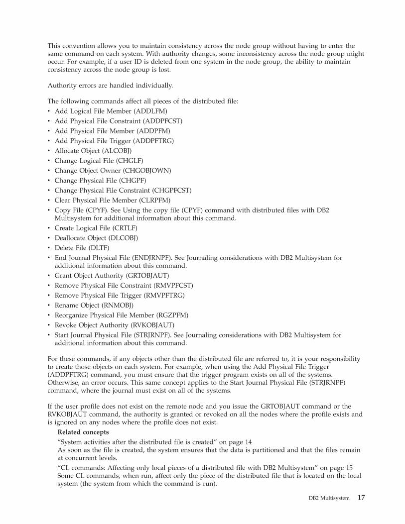
This convention allows you to maintain consistency across the node group without having to enter the
same command on each system. With authority changes, some inconsistency across the node group might
occur. For example, if a user ID is deleted from one system in the node group, the ability to maintain
consistency across the node group is lost.
Authority errors are handled individually.
The following commands affect all pieces of the distributed file:
v Add Logical File Member (ADDLFM)
v Add Physical File Constraint (ADDPFCST)
v Add Physical File Member (ADDPFM)
v Add Physical File Trigger (ADDPFTRG)
v Allocate Object (ALCOBJ)
v Change Logical File (CHGLF)
v Change Object Owner (CHGOBJOWN)
v Change Physical File (CHGPF)
v Change Physical File Constraint (CHGPFCST)
v Clear Physical File Member (CLRPFM)
v Copy File (CPYF). See Using the copy file (CPYF) command with distributed files with DB2
Multisystem for additional information about this command.
v Create Logical File (CRTLF)
v Deallocate Object (DLCOBJ)
v Delete File (DLTF)
v End Journal Physical File (ENDJRNPF). See Journaling considerations with DB2 Multisystem for
additional information about this command.
v Grant Object Authority (GRTOBJAUT)
v Remove Physical File Constraint (RMVPFCST)
v Remove Physical File Trigger (RMVPFTRG)
v Rename Object (RNMOBJ)
v Reorganize Physical File Member (RGZPFM)
v Revoke Object Authority (RVKOBJAUT)
v Start Journal Physical File (STRJRNPF). See Journaling considerations with DB2 Multisystem for
additional information about this command.
For these commands, if any objects other than the distributed file are referred to, it is your responsibility
to create those objects on each system. For example, when using the Add Physical File Trigger
(ADDPFTRG) command, you must ensure that the trigger program exists on all of the systems.
Otherwise, an error occurs. This same concept applies to the Start Journal Physical File (STRJRNPF)
command, where the journal must exist on all of the systems.
If the user profile does not exist on the remote node and you issue the GRTOBJAUT command or the
RVKOBJAUT command, the authority is granted or revoked on all the nodes where the profile exists and
is ignored on any nodes where the profile does not exist.
Related concepts
“System activities after the distributed file is created” on page 14As soon as the file is created, the system ensures that the data is partitioned and that the files remain
at concurrent levels.
“CL commands: Affecting only local pieces of a distributed file with DB2 Multisystem” on page 15Some CL commands, when run, affect only the piece of the distributed file that is located on the local
system (the system from which the command is run).
DB2 Multisystem 17
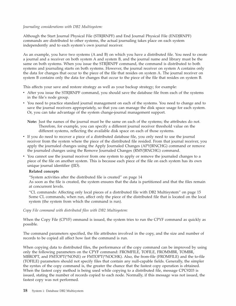
Journaling considerations with DB2 Multisystem:
Although the Start Journal Physical File (STRJRNPF) and End Journal Physical File (ENDJRNPF)
commands are distributed to other systems, the actual journaling takes place on each system
independently and to each system’s own journal receiver.
As an example, you have two systems (A and B) on which you have a distributed file. You need to create
a journal and a receiver on both system A and system B, and the journal name and library must be the
same on both systems. When you issue the STRJRNPF command, the command is distributed to both
systems and journaling starts on both systems. However, the journal receiver on system A contains only
the data for changes that occur to the piece of the file that resides on system A. The journal receiver on
system B contains only the data for changes that occur to the piece of the file that resides on system B.
This affects your save and restore strategy as well as your backup strategy; for example:
v After you issue the STRJRNPF command, you should save the database file from each of the systems
in the file’s node group.
v You need to practice standard journal management on each of the systems. You need to change and to
save the journal receivers appropriately, so that you can manage the disk space usage for each system.
Or, you can take advantage of the system change-journal management support.
Note: Just the names of the journal must be the same on each of the systems; the attributes do not.
Therefore, for example, you can specify a different journal receiver threshold value on the
different systems, reflecting the available disk space on each of those systems.
v If you do need to recover a piece of a distributed database file, you only need to use the journal
receiver from the system where the piece of the distributed file resided. From that journal receiver, you
apply the journaled changes using the Apply Journaled Changes (APYJRNCHG) command or remove
the journaled changes using the Remove Journaled Changes (RMVJRNCHG) command.
v You cannot use the journal receiver from one system to apply or remove the journaled changes to a
piece of the file on another system. This is because each piece of the file on each system has its own
unique journal identifier (JID).
Related concepts
“System activities after the distributed file is created” on page 14As soon as the file is created, the system ensures that the data is partitioned and that the files remain
at concurrent levels.
“CL commands: Affecting only local pieces of a distributed file with DB2 Multisystem” on page 15Some CL commands, when run, affect only the piece of the distributed file that is located on the local
system (the system from which the command is run).
Copy File command with distributed files with DB2 Multisystem:
When the Copy File (CPYF) ommand is issued, the system tries to run the CPYF command as quickly as
possible.
The command parameters specified, the file attributes involved in the copy, and the size and number of
records to be copied all affect how fast the command is run.
When copying data to distributed files, the performance of the copy command can be improved by using
only the following parameters on the CPYF command: FROMFILE, TOFILE, FROMMBR, TOMBR,
MBROPT, and FMTOPT(*NONE) or FMTOPT(*NOCHK). Also, the from-file (FROMFILE) and the to-file
(TOFILE) parameters should not specify files that contain any null-capable fields. Generally, the simpler
the syntax of the copy command is, the greater the chance that the fastest copy operation is obtained.
When the fastest copy method is being used while copying to a distributed file, message CPC9203 is
issued, stating the number of records copied to each node. Normally, if this message was not issued, the
fastest copy was not performed.
18 System i: Database DB2 Multisystem
When copying to a distributed file, you should consider the following differences between when the
fastest copy is and is not used:
v For the fastest copy, records are buffered for each node. As the buffers become full, they are sent to a
particular node. If an error occurs after any records are placed in any of the node buffers, the system
tries to send all of the records currently in the node buffers to their correct node. If an error occurs
while the system is sending records to a particular node, processing continues to the next node until
the system has tried to send all the node buffers.
In other words, records that follow a particular record that is in error can be written to the distributed
file. This action occurs because of the simultaneous blocking done at the multiple nodes. If you do not
want the records that follow a record that is in error to be written to the distributed file, you can force
the fastest copy not to be used by specifying on the CPYF command either ERRLVL(*NOMAX) or
ERRLVL with a value greater than or equal to 1.
When the fastest copy is not used, record blocking is attempted unless the to-file open is or is forced to
become a SEQONLY(*NO) open.
v When the fastest copy is used, a message is issued stating that the opening of the member was
changed to SEQONLY(*NO); however, the distributed to-file is opened a second time to allow for the
blocking of records. You should ignore the message about the change to SEQONLY(*NO).
v When the fastest copy is used, multiple messages are issued stating the number of records copied to
each node. A message is then sent stating the total number of records copied.
v When the fastest copy is not used, only the total number of records copied message is sent. No
messages are sent listing the number of records copied to each node.
Consider the following restrictions when copying to or from distributed files:
v The FROMRCD parameter can be specified only with a value of *START or 1 when copying from a
distributed file. The TORCD parameter cannot be specified with a value other than the default value
*END when copying from a distributed file.
v The MBROPT(*UPDADD) parameter is not allowed when copying to a distributed file.
v The COMPRESS(*NO) parameter is not allowed when the to-file is a distributed file and the from-file
is a database delete-capable file.
v For copy print listings, the RCDNBR value given is the position of the record in the file on a particular
node when the record is a distributed file record. The same record number appears multiple times on
the listing, with each one being a record from a different node.
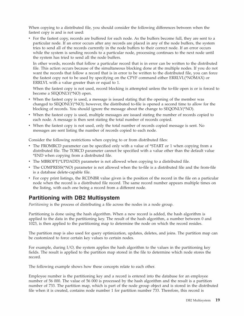
Partitioning with DB2 Multisystem
Partitioning is the process of distributing a file across the nodes in a node group.
Partitioning is done using the hash algorithm. When a new record is added, the hash algorithm is
applied to the data in the partitioning key. The result of the hash algorithm, a number between 0 and
1023, is then applied to the partitioning map to determine the node on which the record resides.
The partition map is also used for query optimization, updates, deletes, and joins. The partition map can
be customized to force certain key values to certain nodes.
For example, during I/O, the system applies the hash algorithm to the values in the partitioning key
fields. The result is applied to the partition map stored in the file to determine which node stores the
record.
The following example shows how these concepts relate to each other.
Employee number is the partitioning key and a record is entered into the database for an employee
number of 56 000. The value of 56 000 is processed by the hash algorithm and the result is a partition
number of 733. The partition map, which is part of the node group object and is stored in the distributed
file when it is created, contains node number 1 for partition number 733. Therefore, this record is
DB2 Multisystem 19
physically stored on the system in the node group that is assigned node number 1. The partitioning key
(the PTNKEY parameter) was specified by you when you created the partitioned (distributed) file.
Fields in the partitioning key can be null-capable. However, records that contain a null value within the
partitioning key always hash to partition number 0. Files with a significant number of null values within
the partitioning key can result in data skew on the partition number 0, because all of the records with
null values hash to partition number 0.
After you have created your node group object and a partitioned distributed relational database file, you
can use the DSPNODGRP command to view the relationship between partition numbers and node
names. In the Displaying node groups using the DSPNODGRP command with DB2 Multisystem topic,
you can find more information about displaying partition numbers, node groups, and system names.
When creating a distributed file, the partitioning key fields are specified either on the PTNKEY parameter
of the Create Physical File (CRTPF) command or in the PARTITIONING KEY clause of the SQL CREATE
TABLE statement. Fields with the data types DATE, TIME, TIMESTAMP, and FLOAT are not allowed in a
partitioning key.
Related concepts
“How node groups work with DB2 Multisystem” on page 5A node group is a system object (*NODGRP), which is stored on the system on which it was created.
“Display Node Group command” on page 8The Display Node Group (DSPNODGRP) command displays the nodes (systems) in a node group.
“Change Node Group Attributes command” on page 10The Change Node Group Attributes (CHGNODGRPA) command changes the data partitioning
attributes for a node group.
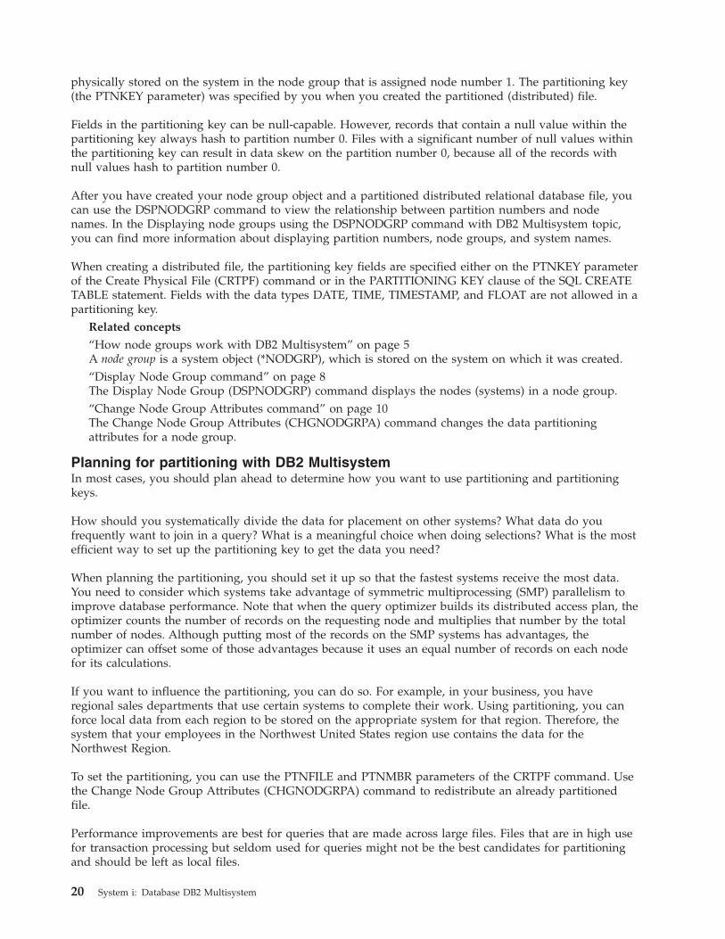
Planning for partitioning with DB2 Multisystem
In most cases, you should plan ahead to determine how you want to use partitioning and partitioning
keys.
How should you systematically divide the data for placement on other systems? What data do you
frequently want to join in a query? What is a meaningful choice when doing selections? What is the most
efficient way to set up the partitioning key to get the data you need?
When planning the partitioning, you should set it up so that the fastest systems receive the most data.
You need to consider which systems take advantage of symmetric multiprocessing (SMP) parallelism to
improve database performance. Note that when the query optimizer builds its distributed access plan, the
optimizer counts the number of records on the requesting node and multiplies that number by the total
number of nodes. Although putting most of the records on the SMP systems has advantages, the
optimizer can offset some of those advantages because it uses an equal number of records on each node
for its calculations.
If you want to influence the partitioning, you can do so. For example, in your business, you have
regional sales departments that use certain systems to complete their work. Using partitioning, you can
force local data from each region to be stored on the appropriate system for that region. Therefore, the
system that your employees in the Northwest United States region use contains the data for the
Northwest Region.
To set the partitioning, you can use the PTNFILE and PTNMBR parameters of the CRTPF command. Use
the Change Node Group Attributes (CHGNODGRPA) command to redistribute an already partitioned
file.
Performance improvements are best for queries that are made across large files. Files that are in high use
for transaction processing but seldom used for queries might not be the best candidates for partitioning
and should be left as local files.
20 System i: Database DB2 Multisystem
For join processing, if you often join two files on a specific field, you should make that field the
partitioning key for both files. You should also ensure that the fields are of the same data type.
Related concepts
SQL programming
Database programming
“Customizing data distribution with DB2 Multisystem” on page 22Because the system is responsible for placing the data, you do not need to know where the records
actually reside. However, if you want to guarantee that certain records are always stored on a
particular system, you can use the Change Node Group Attributes (CHGNODGRPA) command to
specify where those records reside.
Choosing partitioning keys with DB2 Multisystem
For the system to process the partitioned file in the most efficient manner, there are some tips you can
consider when setting up or using a partitioning key.
These tips are as follows:
v The best partitioning key is one that has many different values and, therefore, the partitioning activity
results in an even distribution of the records of data. Customer numbers, last names, claim numbers,
ZIP codes (regional mailing address codes), and telephone area codes are examples of good categories
for using as partitioning keys.
Gender, because only two choices exist, male or female, is an example of a poor choice for a
partitioning key. Gender causes too much data to be distributed to a single node instead of spread
across the nodes. Also, when doing a query, gender as the partitioning key causes the system to
process through too many records of data. It is inefficient; another field or fields of data can narrow the
scope of the query and make it much more efficient. A partitioning key based on gender is a poor
choice in cases where even distribution of data is wanted rather than distribution based on specific
values.
When preparing to change a local file into a distributed file, you can use the HASH function to get an
idea of how the data is distributed. Because the HASH function can be used against local files and
with any variety of columns, you can try different partitioning keys before actually changing the file to
be distributed. For example, if you plan to use the ZIP code field of a file, you can run the HASH
function using that field to get an idea of the number of records that HASH to each partition number.
This helps you in choosing your partitioning key fields, or in creating the partition map in your node
groups.
v Do not choose a field that needs to be updated often. A restriction on partitioning key fields is that
they can have their values updated only if the update does not force the record to a different node.
v Do not use many fields in the partitioning key; the best choice is to use one field. Using many fields
forces the system to do more work at I/O time.
v Choose a simple data type, such as fixed-length character or integer, as your partitioning key. This
consideration might help performance because the hashing is done for a single field of a simple data
type.
v When choosing a partitioning key, you should consider the join and grouping criteria of the queries
you typically run. For example, choosing a field that is never used as a join field for a file that is
involved in joins can adversely affect join performance. See Query design for performance with DB2
Multisystem for information about running queries involving distributed files.
Related concepts
“Query design for performance with DB2 Multisystem” on page 39You can design queries based on these guidelines. In this way, you can use query resources more
efficiently when you run queries that use distributed files.
DB2 Multisystem 21
Customizing data distribution with DB2 Multisystem
Because the system is responsible for placing the data, you do not need to know where the records
actually reside. However, if you want to guarantee that certain records are always stored on a particular
system, you can use the Change Node Group Attributes (CHGNODGRPA) command to specify where
those records reside.
As an example, suppose you want all the records for the 55902 ZIP code to reside on your system in
Minneapolis, Minnesota. When you issue the CHGNODGRPA command, you should specify the 55902
ZIP code and the system node number of the local node in Minneapolis.
At this point, the 55902 ZIP has changed node groups, but the data is still distributed as it was
previously. The CHGNODGRPA command does not affect the existing files. When a partitioned file is
created, the partitioned file keeps a copy of the information from the node group at that time. The node
group can be changed or deleted without affecting the partitioned file. For the changes to the records that
are to be redistributed to take effect, either you can re-create the distributed file using the new node
group, or you can use the Change Physical File (CHGPF) command and specify the new or updated node
group.
Using the CHGPF command, you can:
v Redistribute an already partitioned file
v Change a partitioning key (from the telephone area code to the branch ID, for example)
v Change a local file to be a distributed file
v Change a distributed file to a local file.
Note: You must also use the CHGNODGRPA command to redistribute an already partitioned file. The
CHGNODGRPA command can be optionally used with the CHGPF command to do any of the
other tasks.
In the Redistribution issues for adding systems to a network topic, you can find information on changing
a local file to a distributed file or a distributed file to a local file.
Related concepts
“Change Node Group Attributes command” on page 10The Change Node Group Attributes (CHGNODGRPA) command changes the data partitioning
attributes for a node group.
“Planning for partitioning with DB2 Multisystem” on page 20In most cases, you should plan ahead to determine how you want to use partitioning and partitioning
keys.
“Redistribution issues for adding systems to a network” on page 38The redistribution of a file across a node group is a fairly simple process.
Partitioned tables
DB2 UDB for iSeries supports partitioned tables using SQL.
Partitioning allows for the data to be stored in more than one member, but the table appears as one object
for data manipulation operations, such as queries, inserts, updates, and deletes. The partitions inherit the
design characteristics of the table on which they are based, including the column names and types,
constraints, and triggers.
Partitioning allows you to have much more data in your tables. Without partitioning, there is a maximum
of 4 294 967 288 rows in a table, or a maximum size of 1.7 terabytes. A partitioned table, however, can
have many partitions, with each partition able to have the maximum table size. For more information
about maximum size for partitioned tables, refer to the DB2 UDB for iSeries White Papers.
22 System i: Database DB2 Multisystem
Partitioning can also enhance the performance, recoverability, and manageability of your database. Each
partition can be saved, restored, exported from, imported to, dropped, or reorganized independently of
the other partitions. Additionally, partitioning allows for quickly deleting sets of records grouped in a
partition, rather than processing individual rows of a nonpartitioned table. Dropping a partition provides
significantly better performance than deleting the same rows from a nonpartitioned table.
A partitioned table is a database file with multiple members. A partitioned table is the equivalent of a
database file member. Therefore, most of the CL commands that are used for members are also valid for
each partition of a partitioned table.
You must have DB2 Multisystem installed on your system to take advantage of partitioned tables
support. There are, however, some important differences between DB2 Multisystem and partitioning. DB2
Multisystem provides two ways to partition your data:
v You can create a distributed table to distribute your data across several systems or logical partitions.
v You can create a partitioned table to partition your data into several members in the same database
table on one system.
In both cases, you access the table as if it were not partitioned at all.
Related concepts
“DB2 Multisystem: Basic terms and concepts” on page 3A distributed file is a database file that is spread across multiple System i models. Here are some of the
main concepts regarding the creation and use of distributed files by DB2 Multisystem. Related information
DB2 for i5/OS white papers
Creation of partitioned tables
New partitioned tables can be created using the CREATE TABLE statement.
The table definition must include the table name and the names and attributes of the columns in the
table. The definition might also include other attributes of the table, such as the primary key.
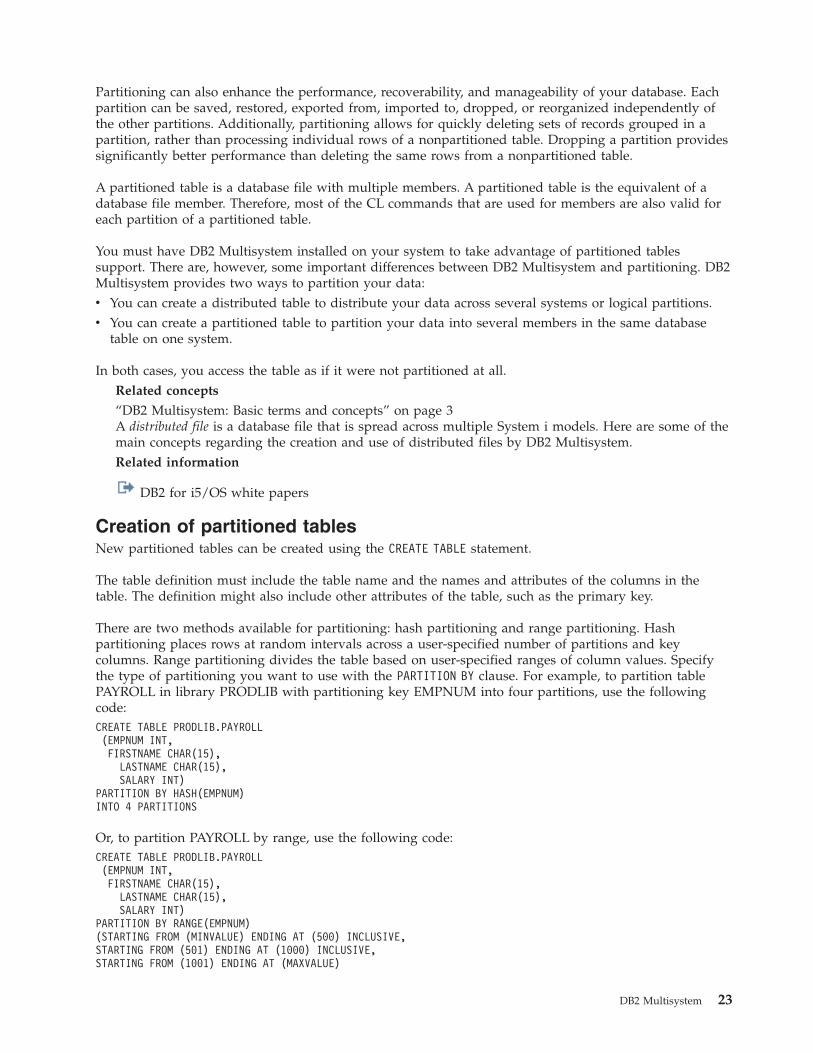
There are two methods available for partitioning: hash partitioning and range partitioning. Hash
partitioning places rows at random intervals across a user-specified number of partitions and key
columns. Range partitioning divides the table based on user-specified ranges of column values. Specify
the type of partitioning you want to use with the PARTITION BY clause. For example, to partition table
PAYROLL in library PRODLIB with partitioning key EMPNUM into four partitions, use the following
code:
CREATE TABLE PRODLIB.PAYROLL
(EMPNUM INT,
FIRSTNAME CHAR(15),
LASTNAME CHAR(15),
SALARY INT)
PARTITION BY HASH(EMPNUM)
INTO 4 PARTITIONS
Or, to partition PAYROLL by range, use the following code:
CREATE TABLE PRODLIB.PAYROLL
(EMPNUM INT,
FIRSTNAME CHAR(15),
LASTNAME CHAR(15),
SALARY INT)
PARTITION BY RANGE(EMPNUM)
(STARTING FROM (MINVALUE) ENDING AT (500) INCLUSIVE,
STARTING FROM (501) ENDING AT (1000) INCLUSIVE,
STARTING FROM (1001) ENDING AT (MAXVALUE)
DB2 Multisystem 23
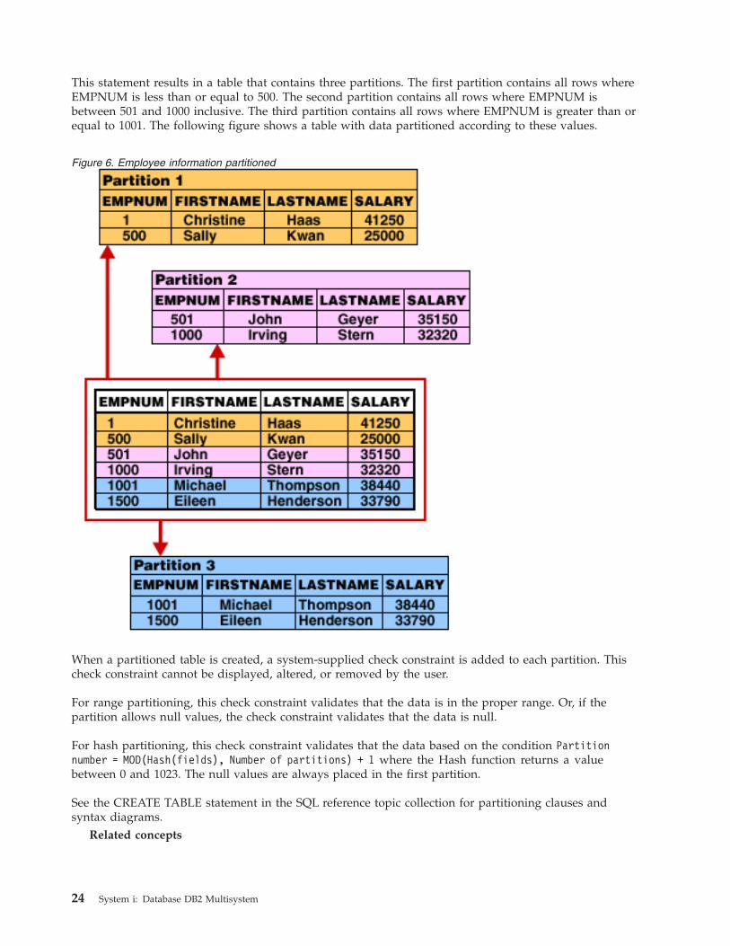
This statement results in a table that contains three partitions. The first partition contains all rows where
EMPNUM is less than or equal to 500. The second partition contains all rows where EMPNUM is
between 501 and 1000 inclusive. The third partition contains all rows where EMPNUM is greater than or
equal to 1001. The following figure shows a table with data partitioned according to these values.
When a partitioned table is created, a system-supplied check constraint is added to each partition. This
check constraint cannot be displayed, altered, or removed by the user.
For range partitioning, this check constraint validates that the data is in the proper range. Or, if the
partition allows null values, the check constraint validates that the data is null.
For hash partitioning, this check constraint validates that the data based on the condition Partition
number = MOD(Hash(fields), Number of partitions) + 1 where the Hash function returns a value
between 0 and 1023. The null values are always placed in the first partition.
See the CREATE TABLE statement in the SQL reference topic collection for partitioning clauses and
syntax diagrams.
Related concepts
Figure 6. Employee information partitioned
24 System i: Database DB2 Multisystem
“From a nonpartitioned table to a partitioned table”Use the ADD partitioning-clause of the ALTER TABLE statement to change a nonpartitioned table
into a partitioned table. Altering an existing table to use partitions is similar to creating a new
partitioned table. Related tasks
CREATE TABLE Related reference
SQL reference
“Check constraint optimization” on page 29The optimizer uses check constraints (either user-added or the implicit check constraints added for the
partition key) to reduce the partitions examined.
Modification of existing tables
You can change existing nonpartitioned tables to partitioned tables, change the attributes of existing
partitioned tables, or change partitioned table to nonpartitioned tables.
Use the ALTER TABLE statement to make changes to partitioned and nonpartitioned tables.
More details about the ALTER TABLE statement and its clauses are available in the SQL reference topic
collection.
Related reference
ALTER TABLE
SQL reference
From a nonpartitioned table to a partitioned table
Use the ADD partitioning-clause of the ALTER TABLE statement to change a nonpartitioned table into a
partitioned table. Altering an existing table to use partitions is similar to creating a new partitioned table.
For example, to add range partitioning to the nonpartitioned table PAYROLL, use the following code:
ALTER TABLE PRODLIB.PAYROLL
ADD PARTITION BY RANGE(EMPNUM)
(STARTING(MINVALUE) ENDING(500) INCLUSIVE,
STARTING(501) ENDING(1000) INCLUSIVE,
STARTING(1001) ENDING MAXVALUE))
Related concepts
“Creation of partitioned tables” on page 23New partitioned tables can be created using the CREATE TABLE statement.
Modification of existing partitioned tables
You can make several changes to your partitioned table by using the clauses of the ALTER TABLE
statement.
These clauses are as follows:
v ADD PARTITION
This clause adds one or more new hash partitions or a range partition to an existing partitioned table.
Make sure that the parameters you specify do not violate the following rules; otherwise, errors occur.
– Do not use the ADD PARTITION clause for nonpartitioned tables.
– When adding hash partitions, the number of partitions being added must be specified as a positive
integer.
– If you supply a name or integer to identify the partition, ensure that it is not already in use by
another partition.
DB2 Multisystem 25
– When adding range partitions, the specified ranges must not overlap the ranges of any existing
partitions.
For example, to alter the table PAYROLL in library PRODLIB with partition key EMPNUM to have
four additional partitions, use the following code:
ALTER TABLE PRODLIB.PAYROLL
ADD PARTITION 4 HASH PARTITIONS
v ALTER PARTITION
This clause alters the range for the identified range partition. Ensure that the following conditions are
met:
– The identified partition must exist in the table.
– The specified ranges must not overlap the ranges of any existing partitions.
– All existing rows of the partitioned table must fall within the new ranges specified on the ALTER
TABLE statement.v DROP PARTITION
This clause drops a partition of a partitioned table. If the specified table is not a partitioned table, an
error is returned. If the last remaining partition of a partitioned table is specified, an error is returned.
Restrictions when altering a column’s data type:
When altering a column’s data type, and that column is part of a partitioning key, there are some
restrictions on the target data type.
For range partitioning, the data type of a column used to partition a table cannot be changed to BLOB,
CLOB, DBCLOB, DATALINK, floating-point type, or a distinct type based on the these types. For hash
partitioning, the data type of the column used as part of the partition key cannot be changed to LOB,
DATE, TIME, TIMESTAMP, floating-point type, or a distinct type based on one of these.
Related reference
ALTER TABLE
From a partitioned table to a nonpartitioned table
The DROP PARTITIONING clause changes a partitioned table to a nonpartitioned table.
If the specified table is already nonpartitioned, an error is returned. Changing a partitioned table that
contains data into a nonpartitioned table requires data movement between the data partitions. You cannot
change a partitioned table whose size is larger than the maximum nonpartitioned table size to a
nonpartitioned table.
Indexes with partitioned tables
Indexes can be created as partitioned or nonpartitioned. A partitioned index creates an individual index
for each partition. A nonpartitioned index is a single index spanning all partitions of the table.
Partitioned indexes allow you to take advantage of improved optimization of queries. If a unique index is
partitioned, columns specified in the index must be the same or a superset of the data partition key.
Use the CREATE INDEX statement to create indexes on partitioned tables. To create an index for each
partition, use the PARTITIONED clause.
CREATE INDEX PRODLIB.SAMPLEINDEX
ON PRODLIB.PAYROLL(EMPNUM) PARTITIONED
To create a single index that spans all partitions, use the NOT PARTITIONED clause.
CREATE INDEX PRODLIB.SAMPLEINDEX
ON PRODLIB.PAYROLL(EMPNUM) NOT PARTITIONED
26 System i: Database DB2 Multisystem
You can only create a partitioned Encoded Vector Index (EVI) over a partitioned table. You cannot create
a nonpartitioned EVI over a partitioned table.
In the CREATE INDEX statement in the SQL reference topic collection, you can find more information
about creating indexes for partitioned tables.
When creating an SQL unique index, unique constraint, or primary key constraint for a partitioned table,
the following restrictions apply:
v An index can be partitioned if the keys of the unique index are the same or a superset of the
partitioned keys.
v If a unique index is created with the default value of NOT PARTITIONED, and the keys of the unique
index are a superset of the partitioned keys, the unique index is created as partitioned. If, however, the
user explicitly specifies NOT PARTITIONED, and the keys of the unique index are a superset of the
partitioned keys, the unique index is created as not partitioned.
Related concepts
“Query performance and optimization”Queries that reference partitioned tables need to be carefully considered because partitioned tables are
often very large. It is important to understand the effects of accessing multiple partitions on your
system and applications. Related tasks
CREATE INDEX Related reference
SQL reference
Query performance and optimization
Queries that reference partitioned tables need to be carefully considered because partitioned tables are
often very large. It is important to understand the effects of accessing multiple partitions on your system
and applications.
Partitioned tables can take advantage of all optimization and parallel processing available using SQL on
DB2 Universal Database™ for iSeries. For general information about query optimization, see the Database
performance and optimization. For partitioned tables, all the data access methods described in the
Database performance and optimization topic can be used to access the data in each partition. In
addition, if the DB2 UDB Symmetric Multiprocessing feature is installed, the parallel data access methods
are available for the optimizer to consider when implementing the query.
If queries need to access only an individual partition in a partitioned table, creating an alias for that
individual partition and then using that alias in the query can enhance performance. The query acts as a
nonpartitioned table query.
Partitioned tables conceptually implemented as a nested table where each partition is unioned to the
other partitions.
For example, if you perform the following query:
SELECT LASTNAME, SALARY FROM PRODLIB.PAYROLL
WHERE SALARY > 20000
The implementation of the query can be described as:
SELECT LASTNAME, SALARY FROM
(SELECT LASTNAME, SALARY FROM PRODLB.PAYROLL(PART00001)
UNION ALL
SELECT LASTNAME, SALARY FROM PRODLB.PAYROLL(PART00002)
DB2 Multisystem 27
UNION ALL
SELECT LASTNAME, SALARY FROM PRODLB.PAYROLL(PART00003))
X (LASTNAME, SALARY)
WHERE X.SALARY > 20000
The implementation of partitioned table queries depends on which query engine is used: the Classic
Query Engine (CQE) or the SQL Query Engine (SQE). You can find more information about the query
engines in the SQE and CQE Engines topic in the Database performance and optimization topic
collection. There are different considerations for each engine.
Related concepts
“Indexes with partitioned tables” on page 26Indexes can be created as partitioned or nonpartitioned. A partitioned index creates an individual
index for each partition. A nonpartitioned index is a single index spanning all partitions of the table.
SQE and CQE Engines Related information
Performance and query optimization
Queries using SQL Query Engine
The SQL Query Engine (SQE) provides targeted optimization for partitioned tables using dynamic
partition expansion optimization.
This targeted optimization method first determines whether a given query is structured such that certain
partitions in the partitioned table would benefit from specific optimization. If targeted optimization is
warranted, the optimizer determines which partitions can benefit from individual optimization; those
partitions are then optimized separately. The remaining partitions use the once for all technique.
The optimizer determines whether the query or table environment justifies dynamic expansion based on
the following characteristics:
v The table is range partitioned and the query involves predicate selection against the range.
v The table has an index over one or some of the partitions, but not all (a subpartition spanning index).
v The table has relatively few partitions.
v Constraint definitions on the table dictate that only certain partitions participate.
v Estimated run time exceeds a particular threshold.
If expansion is justified, the optimizer determines the target partitions using existing statistic techniques
as appropriate. For example, for range partitioning and predicate selection, the optimizer looks into the
statistics or index to determine which main partitions are of interest. When the target partitions are
identified, the optimizer rewrites the query. The target partitions are redefined in a UNION operation.
The remaining partitions remain as a single table instance. That single instance is then added to the
UNION operation along with the target partitions. As soon as the rewriting is performed, the optimizer
uses existing optimization techniques to determine the plan for each UNION piece. At the end of the
optimization, the single instance is converted into another UNION operation of its contained partitions.
The optimized plan for the single instance is replicated across the UNION subtrees, thus drastically
reducing the optimization time for partitioned tables.
The SQL Query Engine also uses logical partition elimination to optimize partitioned tables. This method
allows the optimizer to identify potential partition elimination opportunities. The optimizer looks for
opportunities where a source table’s reduced answer set can be applied to the partition table’s definition
key with a join predicate. When these opportunities are identified, the optimizer builds logic into the
query run time to eliminate partitions based on the result set of the source table.
For example, consider a query in which the optimizer identifies a predicate (in this example, a WHERE
clause) involving the partition key of the partition table. If a constraint on a partition limits the key to a
range from 0 to 10 and a predicate in the query identifies a key value of 11, the partition can be logically
28 System i: Database DB2 Multisystem
|||
||||
||
|
|
|
|
|
||||||||||
|||||
|||
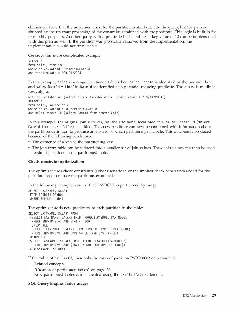
eliminated. Note that the implementation for the partition is still built into the query, but the path is
shunted by the up-front processing of the constraint combined with the predicate. This logic is built in for
reusability purposes. Another query with a predicate that identifies a key value of 10 can be implemented
with this plan as well. If the partition was physically removed from the implementation, the
implementation would not be reusable.
Consider this more complicated example:
select *
from sales, timeDim
where sales.DateId = timeDim.DateId
and timeDim.Date > ’09/01/2004’
In this example, sales is a range-partitioned table where sales.DateId is identified as the partition key
and sales.DateId = timeDim.DateId is identified as a potential reducing predicate. The query is modified
(roughly) as:
with sourceTable as (select * from timeDim where timeDim.Date > ’09/01/2004’)
select *
from sales, sourceTable
where sales.DateId = sourceTable.DateId
and sales.DateId IN (select DateId from sourceTable)
In this example, the original join survives, but the additional local predicate, sales.DateId IN (select
DateId from sourceTable), is added. This new predicate can now be combined with information about
the partition definition to produce an answer of which partitions participate. This outcome is produced
because of the following conditions:
v The existence of a join to the partitioning key.
v The join from table can be reduced into a smaller set of join values. These join values can then be used
to shunt partitions in the partitioned table.
Check constraint optimization:
The optimizer uses check constraints (either user-added or the implicit check constraints added for the
partition key) to reduce the partitions examined.
In the following example, assume that PAYROLL is partitioned by range:
SELECT LASTNAME, SALARY
FROM PRODLIB.PAYROLL
WHERE EMPNUM = :hv1
The optimizer adds new predicates to each partition in the table:
SELECT LASTNAME, SALARY FROM
(SELECT LASTNAME, SALARY FROM PRODLB.PAYROLL(PART00001)
WHERE EMPNUM=:hv1 AND :hv1 <= 500
UNION ALL
SELECT LASTNAME, SALARY FROM PRODLB.PAYROLL(PART00002)
WHERE EMPNUM=:hv1 AND :hv1 >= 501 AND :hv1 <=1000
UNION ALL
SELECT LASTNAME, SALARY FROM PRODLB.PAYROLL(PART00003)
WHERE EMPNUM=:hv1 AND (:hv1 IS NULL OR :hv1 >= 1001))
X (LASTNAME, SALARY)
If the value of hv1 is 603, then only the rows of partition PART00002 are examined.
Related concepts
“Creation of partitioned tables” on page 23New partitioned tables can be created using the CREATE TABLE statement.
SQL Query Engine: Index usage:
DB2 Multisystem 29
|||||
|
||||
|||
|||||
||||
|
||
|
||
|
|||
|
||||||||||
|
|
||
|
The SQL Query Engine (SQE) uses both partitioned and nonpartitioned indexes to implement queries.
If a nonpartitioned index is used, the optimizer can choose to implement the nonpartitioned index for
each partition. This implies that, for example, even if the nonpartitioned index is unique, each partition is
probed for the row.
Queries using Classic Query Engine
When queries are implemented using Classic Query Engine (CQE), you need to be aware of how the
query is optimized including materialization and index usage.
Materialization:
When running Classic Query Engine (CQE), a partitioned table is materialized under some conditions.
These conditions are:
v It is a part of a join query.
v It has a GROUP BY clause.
v It has a column built-in function.
In order to reduce the size of the temporary table and reduce the run time involved for the query, any
selection in the query that can be used during the creation of the temporary table to eliminate rows is
processed to decrease the size of the temporary table and reduce processing time during materialization
cases.
Note: When the partitioned table is materialized, the size of the temporary table cannot exceed 4 294 967
288 rows. Pushdown of selection processing is performed to limit the number of rows in the
temporary table. If the number of rows exceeds 4 294 967 288, a resource limit error is issued and
the query ends.
CQE query optimization considerations:
The Classic Query Engine (CQE) optimizer optimizes the query using the first partition member in the
partitioned table. This access method is used to access rows from all of the partitions.
DB2 UDB Symmetric Multiprocessing feature data access methods cannot be used to access a partitioned
table, but they can be used when processing temporary tables and for creating temporary indexes.
If the partitioned table is used in a query containing a subquery, the optimizer does not attempt to
implement the query as a join composite query. This keeps the partitioned table from being materialized
because of the join.
Classic Query Engine: Index usage:
The Classic Query Engine (CQE) uses nonpartitioned indexes to implement queries.
If a partitioned index exists, the optimizer does not use the index to make optimization decisions
concerning the access method to use while processing the partition table.
The optimizer creates temporary indexes over partitioned tables allowing update of live data with
ordering.
Because encoded vector indexes (EVIs) are only created over a single partition, CQE cannot use EVIs to
implement partitioned table queries.
30 System i: Database DB2 Multisystem
|
|||
Save and restore considerations
A partitioned table can be saved and restored just as any other database file.
The partitions of a partitioned table are database members, and hence can be saved and restored together
or individually. Consider the following items when saving and restoring partitioned tables.
v If you restore only some of the partitions of a partitioned table to a system where the partitioned table
did not previously exist, the system creates the partitions that you did not restore. The created
partitions that were not restored cannot have any data restored.
v If you save a table partitioned by range, then drop one or more partitions, you are able to restore the
dropped partitions to the partitioned table.
v If you save a table partitioned by hash, then alter the table by dropping or adding partitions, you are
not be able to restore the table that was saved to the table on the system. If, however, the table on the
system is deleted, you can restore the table that was saved.
Applications using the following save and restore CL commands must be changed to use Member *ALL to
process all partitions of a partitioned table:
v Restore Object (RSTOBJ)
v Save Object (SAVOBJ)
v Save Restore Object (SAVRSTOBJ)
Related tasks
Database backup and recovery
Journaling a partitioned table
You can journal a partitioned table as you can journal any other database file with multiple members.
When you journal a partitioned table, all the partitions of the table are journaled by the same journal.
Applications using the following journaling CL commands must be changed to use Member *ALL to
process all partitions of a partitioned table:
v Apply Journaled Changes (APYJRNCHG)
v Apply Journaled Changes Extend (APYJRNCHGX)
v Display Journal (DSPJRN)
v Receive Journal Entry (RCVJRNE)
v Remove Journaled Changes (RMVJRNCHG)
v Retrieve Journal Entry (RTVJRNE)
Related concepts
Journal management
Traditional system interface considerations
An SQL table is a database physical file with one member (partition). Therefore, when the file is accessed
by a traditional system application, the traditional system application reads and writes to the member by
opening the file’s member.
When the file (SQL table) becomes partitioned, the file becomes a multimember file and the traditional
system application needs to specify the member name (partition name). The traditional system
application can avoid having to specify a member name when reading or writing data by changing the
application to use an SQL index that is based on all the members of the physical file.
For example, if the user created an SQL index with the following code,
CREATE INDEX LIBNAME.INDEXNAME
ON LIBNAME.TABLENAME(COLUMNNAME)
NOT PARTITIONED
DB2 Multisystem 31
The traditional system application can read and write data from the partitioned table without having to
know how the data is partitioned.
When the table becomes partitioned (becomes a multimember file), any traditional system operation that
was previously done to the table must be done for each member of the multimember file. For example,
RGZPFM FILE(LIBNAME/TABLENAME) only reorganizes the *FIRST member. For a partitioned table,
you need to use the Reorganize Physical File Member (RGZPFM) command for each member. The
Display File Description (DSPFD) command, DSPFD FILE(LIBNAME/TABLENAME) TYPE(*MBRLIST),
lists all members of the file.
Related reference
Reorganize Physical File Member (RGZPFM) command
Display File Description (DSPFD) command
Restrictions for a partitioned table
When you use partitioned tables, be aware of these restrictions.
v Referential constraints are not allowed for a partitioned table.
v If a primary key constraint for a partitioned table is added and then dropped, the primary key index is
also dropped.
v If a primary key constraint is added to a partitioned table, and then removed by the user, the user is
not allowed to keep the table keyed.
v If an existing nonpartitioned table does not have a primary key constraint, but the table is keyed, the
keys are removed when the table is changed to a partitioned table.
v DB2 Multisystem files (distributed tables) are already partitioned across multiple systems and cannot
be partitioned across multiple members on a single system.
v An update to the partitioning key that attempts to move a row to a different partition is not allowed.
v The number of partitioning keys is restricted to 120.
v All SQL relative record processing is handled as it is for DB2 Multisystem support. The relative record
number is determined in each individual partition, not the table as a whole. For example, reading to
record 27 means that you read to record 27 in each partition. Each partition can contain its own record
27, none of which is the same.
v There are some restrictions on the data type of a partition key column. For range partitioning, the data
type of a column used to partition a table cannot be BLOB, CLOB, DBCLOB, DATALINK,
floating-point type, or a distinct type based on the these types. For hash partitioning, the data type of
the column used as part of the partition key cannot be LOB, DATE, TIME, TIMESTAMP, floating-point
type, or a distinct type based on one of these.
v Applications using the following CL commands must be changed to use Member *ALL to process all
partitions of a partitioned table:
– Clear Physical File Member (CLRPFM)
– Copy from Import File (CPYFRMIMPF)
– Copy to Import File (CPYTOIMPF)
– Delete Network File (DLTNETF)
– Open Query File (OPNQRYF)
– Run Query (RUNQRY)
– Work with Object Locks (WRKOBJLCK)
– Apply Journaled Changes (APYJRNCHG)
– Apply Journaled Changes Extend (APYJRNCHGX)
– Display Journal (DSPJRN)
– Receive Journal Entry (RCVJRNE)
– Remove Journaled Changes (RMVJRNCHG)
32 System i: Database DB2 Multisystem
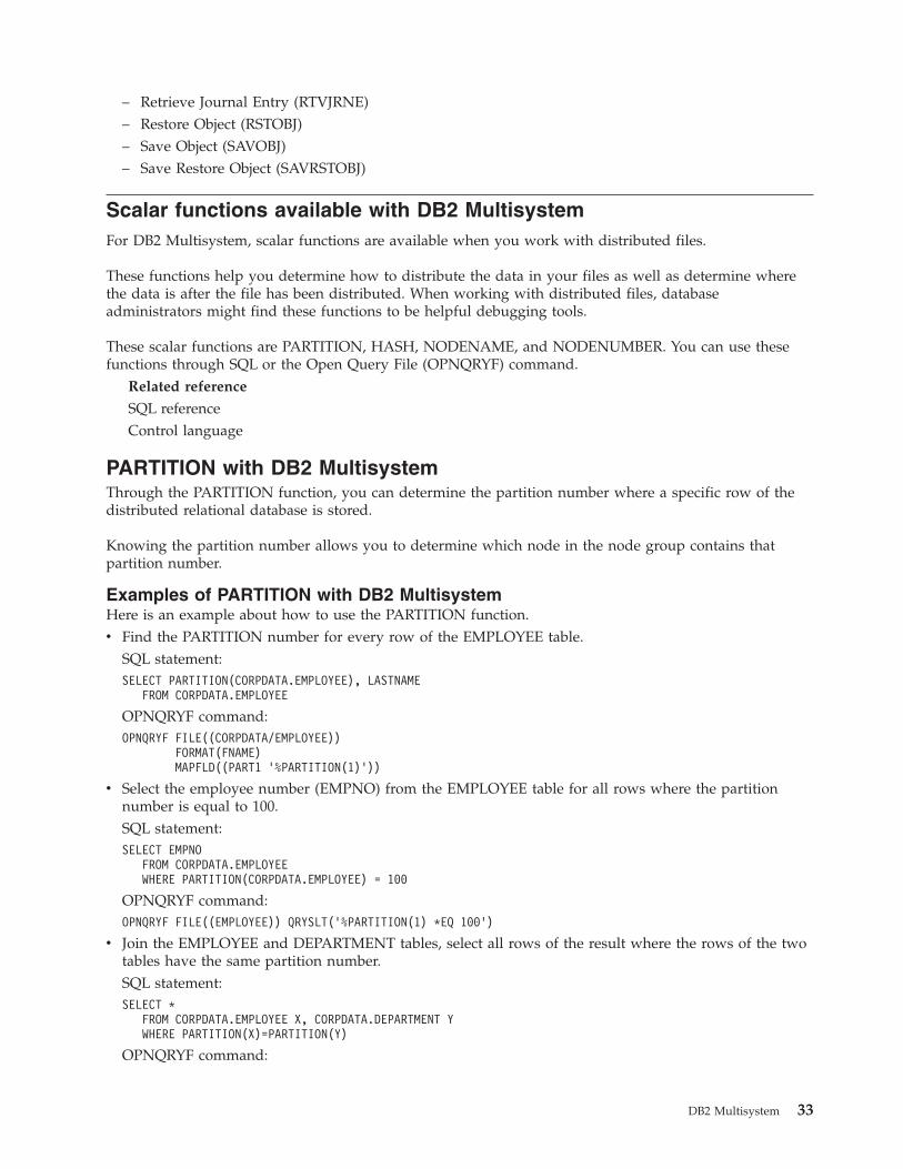
– Retrieve Journal Entry (RTVJRNE)
– Restore Object (RSTOBJ)
– Save Object (SAVOBJ)
– Save Restore Object (SAVRSTOBJ)
Scalar functions available with DB2 Multisystem
For DB2 Multisystem, scalar functions are available when you work with distributed files.
These functions help you determine how to distribute the data in your files as well as determine where
the data is after the file has been distributed. When working with distributed files, database
administrators might find these functions to be helpful debugging tools.
These scalar functions are PARTITION, HASH, NODENAME, and NODENUMBER. You can use these
functions through SQL or the Open Query File (OPNQRYF) command.
Related reference
SQL reference
Control language
PARTITION with DB2 Multisystem
Through the PARTITION function, you can determine the partition number where a specific row of the
distributed relational database is stored.
Knowing the partition number allows you to determine which node in the node group contains that
partition number.
Examples of PARTITION with DB2 Multisystem
Here is an example about how to use the PARTITION function.
v Find the PARTITION number for every row of the EMPLOYEE table.
SQL statement:
SELECT PARTITION(CORPDATA.EMPLOYEE), LASTNAME
FROM CORPDATA.EMPLOYEE
OPNQRYF command:
OPNQRYF FILE((CORPDATA/EMPLOYEE))
FORMAT(FNAME)
MAPFLD((PART1 ’%PARTITION(1)’))
v Select the employee number (EMPNO) from the EMPLOYEE table for all rows where the partition
number is equal to 100.
SQL statement:
SELECT EMPNO
FROM CORPDATA.EMPLOYEE
WHERE PARTITION(CORPDATA.EMPLOYEE) = 100
OPNQRYF command:
OPNQRYF FILE((EMPLOYEE)) QRYSLT(’%PARTITION(1) *EQ 100’)
v Join the EMPLOYEE and DEPARTMENT tables, select all rows of the result where the rows of the two
tables have the same partition number.
SQL statement:
SELECT *
FROM CORPDATA.EMPLOYEE X, CORPDATA.DEPARTMENT Y
WHERE PARTITION(X)=PARTITION(Y)
OPNQRYF command:
DB2 Multisystem 33
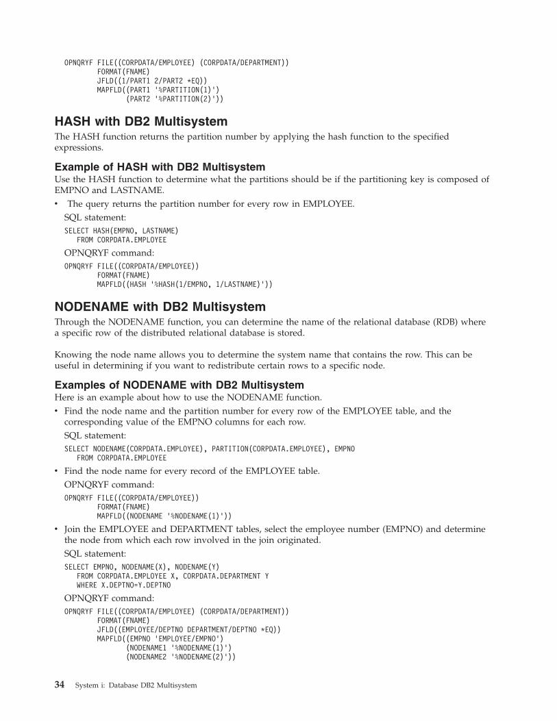
OPNQRYF FILE((CORPDATA/EMPLOYEE) (CORPDATA/DEPARTMENT))
FORMAT(FNAME)
JFLD((1/PART1 2/PART2 *EQ))
MAPFLD((PART1 ’%PARTITION(1)’)
(PART2 ’%PARTITION(2)’))
HASH with DB2 Multisystem
The HASH function returns the partition number by applying the hash function to the specified
expressions.
Example of HASH with DB2 Multisystem
Use the HASH function to determine what the partitions should be if the partitioning key is composed of
EMPNO and LASTNAME.
v The query returns the partition number for every row in EMPLOYEE.
SQL statement:
SELECT HASH(EMPNO, LASTNAME)
FROM CORPDATA.EMPLOYEE
OPNQRYF command:
OPNQRYF FILE((CORPDATA/EMPLOYEE))
FORMAT(FNAME)
MAPFLD((HASH ’%HASH(1/EMPNO, 1/LASTNAME)’))
NODENAME with DB2 Multisystem
Through the NODENAME function, you can determine the name of the relational database (RDB) where
a specific row of the distributed relational database is stored.
Knowing the node name allows you to determine the system name that contains the row. This can be
useful in determining if you want to redistribute certain rows to a specific node.
Examples of NODENAME with DB2 Multisystem
Here is an example about how to use the NODENAME function.
v Find the node name and the partition number for every row of the EMPLOYEE table, and the
corresponding value of the EMPNO columns for each row.
SQL statement:
SELECT NODENAME(CORPDATA.EMPLOYEE), PARTITION(CORPDATA.EMPLOYEE), EMPNO
FROM CORPDATA.EMPLOYEE
v Find the node name for every record of the EMPLOYEE table.
OPNQRYF command:
OPNQRYF FILE((CORPDATA/EMPLOYEE))
FORMAT(FNAME)
MAPFLD((NODENAME ’%NODENAME(1)’))
v Join the EMPLOYEE and DEPARTMENT tables, select the employee number (EMPNO) and determine
the node from which each row involved in the join originated.
SQL statement:
SELECT EMPNO, NODENAME(X), NODENAME(Y)
FROM CORPDATA.EMPLOYEE X, CORPDATA.DEPARTMENT Y
WHERE X.DEPTNO=Y.DEPTNO
OPNQRYF command:
OPNQRYF FILE((CORPDATA/EMPLOYEE) (CORPDATA/DEPARTMENT))
FORMAT(FNAME)
JFLD((EMPLOYEE/DEPTNO DEPARTMENT/DEPTNO *EQ))
MAPFLD((EMPNO ’EMPLOYEE/EMPNO’)
(NODENAME1 ’%NODENAME(1)’)
(NODENAME2 ’%NODENAME(2)’))
34 System i: Database DB2 Multisystem
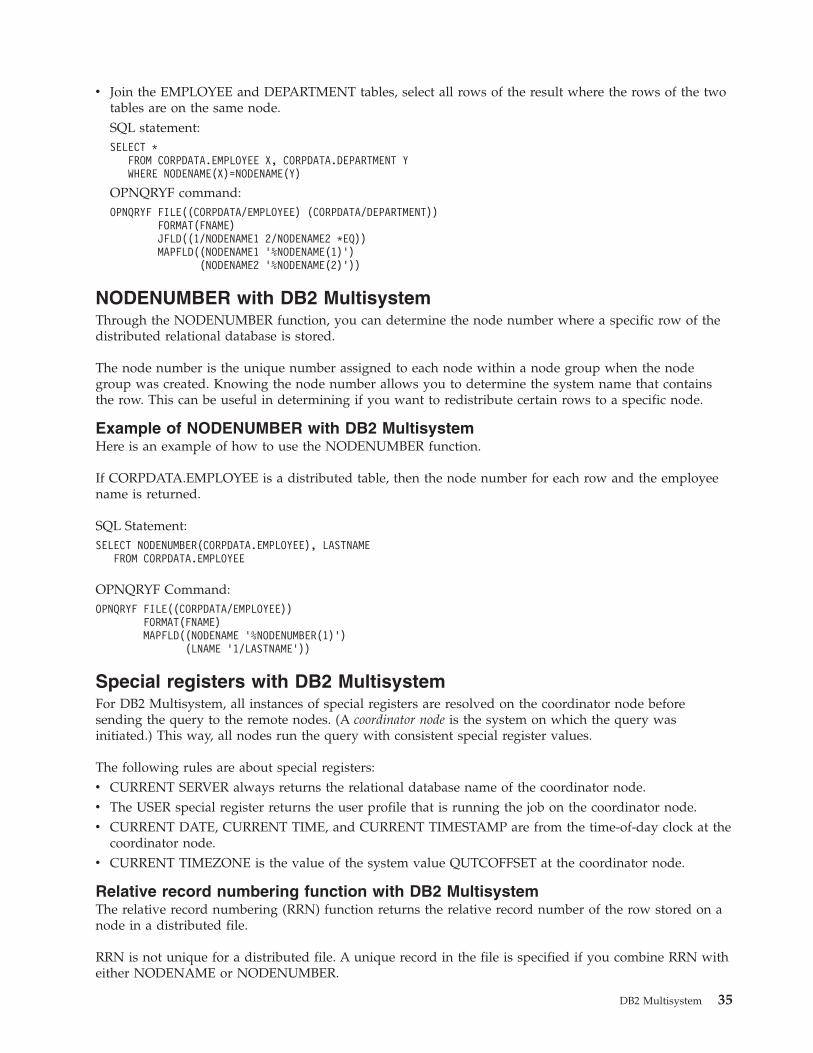
v Join the EMPLOYEE and DEPARTMENT tables, select all rows of the result where the rows of the two
tables are on the same node.
SQL statement:
SELECT *
FROM CORPDATA.EMPLOYEE X, CORPDATA.DEPARTMENT Y
WHERE NODENAME(X)=NODENAME(Y)
OPNQRYF command:
OPNQRYF FILE((CORPDATA/EMPLOYEE) (CORPDATA/DEPARTMENT))
FORMAT(FNAME)
JFLD((1/NODENAME1 2/NODENAME2 *EQ))
MAPFLD((NODENAME1 ’%NODENAME(1)’)
(NODENAME2 ’%NODENAME(2)’))
NODENUMBER with DB2 Multisystem
Through the NODENUMBER function, you can determine the node number where a specific row of the
distributed relational database is stored.
The node number is the unique number assigned to each node within a node group when the node
group was created. Knowing the node number allows you to determine the system name that contains
the row. This can be useful in determining if you want to redistribute certain rows to a specific node.
Example of NODENUMBER with DB2 Multisystem
Here is an example of how to use the NODENUMBER function.
If CORPDATA.EMPLOYEE is a distributed table, then the node number for each row and the employee
name is returned.
SQL Statement:
SELECT NODENUMBER(CORPDATA.EMPLOYEE), LASTNAME
FROM CORPDATA.EMPLOYEE
OPNQRYF Command:
OPNQRYF FILE((CORPDATA/EMPLOYEE))
FORMAT(FNAME)
MAPFLD((NODENAME ’%NODENUMBER(1)’)
(LNAME ’1/LASTNAME’))
Special registers with DB2 Multisystem
For DB2 Multisystem, all instances of special registers are resolved on the coordinator node before
sending the query to the remote nodes. (A coordinator node is the system on which the query was
initiated.) This way, all nodes run the query with consistent special register values.
The following rules are about special registers:
v CURRENT SERVER always returns the relational database name of the coordinator node.
v The USER special register returns the user profile that is running the job on the coordinator node.
v CURRENT DATE, CURRENT TIME, and CURRENT TIMESTAMP are from the time-of-day clock at the
coordinator node.
v CURRENT TIMEZONE is the value of the system value QUTCOFFSET at the coordinator node.
Relative record numbering function with DB2 Multisystem
The relative record numbering (RRN) function returns the relative record number of the row stored on a
node in a distributed file.
RRN is not unique for a distributed file. A unique record in the file is specified if you combine RRN with
either NODENAME or NODENUMBER.
DB2 Multisystem 35

Performance and scalability with DB2 Multisystem
DB2 Multisystem can help you increase your database capacity, realize improvements in query
performance, and provide remote database access through an easier method.
Using DB2 Multisystem, your users and your applications only need to access the file from the local
system. You have no need to make any code changes to be able to access data in a distributed file versus
a local file. With functions like Distributed Relational Database Architecture (DRDA) and distributed data
management (DDM), your access must be explicitly directed to a remote file or to a remote system to be
able to access that remote data. DB2 Multisystem handles the remote access in such a way that it is
transparent to your users.
DB2 Multisystem also provides a simple growth path for your database expansion.
Why you should use DB2 Multisystem
Performance improvements can be quite significant for certain queries.
Testing has shown that for queries that have a large amount of data to be processed, but with a relatively
small result set, the performance gain is almost proportional to the number of systems the file is
distributed across. For example, suppose you have a 5 million (5 000 000) record file that you want to
query for the top 10 revenue producers. With DB2 Multisystem, the response time for the query is cut by
nearly one-half by partitioning the file equally across two systems. On three systems, the response time is
nearly one-third the time of running the query on a single system. This best case scenario does not apply
to complex join operations where data needs to be moved between nodes.
If a file is fairly small or is primarily used for single-record read or write processing, little or no
performance gain can be realized from partitioning the file. Instead, a slight degradation in performance
might occur. In these cases, query performance becomes more dependent on the speed of the physical
connection. However, even in these situations, the users on all the systems in the node group still have
the advantage of being able to access the data, even though it is distributed, using the traditional local
file database methods with which they are familiar. In all environments, users have the benefits of this
local-system transparency and the possible elimination of data redundancy across the systems in the node
group.
Another parallelism feature, DB2 UDB Symmetric Multiprocessing, can also increase performance. With
symmetric multiprocessing (SMP), when a partitioned file is processed and if any of the systems are
multiprocessor systems, you can achieve a multiplier effect in terms of performance gains. If you
partitioned a file across three systems and each system is a 4-way processor system, the functions of DB2
Multisystem and SMP work together. Using the previous 5 million record example, the response time is
approximately one-twelfth of what it would have been had the query been run without using any of the
parallelism features. The file sizes and the details of the query can affect the improvement that you
actually see.
When you do queries, the bulk of the work to run the query is done in parallel, which improves the
overall performance of query processing. The system divides up the query and processes the appropriate
parts of the query on the appropriate system. This makes for the most efficient processing, and it is done
automatically; you do not need to specify anything to make this highly efficient processing occur.
Note: The performance of some queries might not improve, especially if a large volume of data has to be
moved.
Each node only has to process the records that are physically stored on that node. If the query specifies
selection against the partitioning key, the query optimizer might determine that only one node needs to
be queried. In the following example, the ZIP code field is the partitioning key within the SQL statement
for the ORDERS file:
36 System i: Database DB2 Multisystem
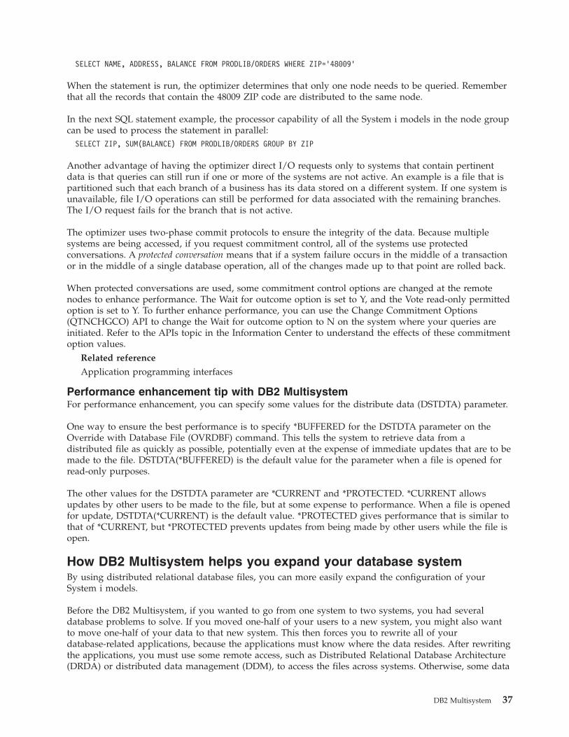
SELECT NAME, ADDRESS, BALANCE FROM PRODLIB/ORDERS WHERE ZIP=’48009’
When the statement is run, the optimizer determines that only one node needs to be queried. Remember
that all the records that contain the 48009 ZIP code are distributed to the same node.
In the next SQL statement example, the processor capability of all the System i models in the node group
can be used to process the statement in parallel:
SELECT ZIP, SUM(BALANCE) FROM PRODLIB/ORDERS GROUP BY ZIP
Another advantage of having the optimizer direct I/O requests only to systems that contain pertinent
data is that queries can still run if one or more of the systems are not active. An example is a file that is
partitioned such that each branch of a business has its data stored on a different system. If one system is
unavailable, file I/O operations can still be performed for data associated with the remaining branches.
The I/O request fails for the branch that is not active.
The optimizer uses two-phase commit protocols to ensure the integrity of the data. Because multiple
systems are being accessed, if you request commitment control, all of the systems use protected
conversations. A protected conversation means that if a system failure occurs in the middle of a transaction
or in the middle of a single database operation, all of the changes made up to that point are rolled back.
When protected conversations are used, some commitment control options are changed at the remote
nodes to enhance performance. The Wait for outcome option is set to Y, and the Vote read-only permitted
option is set to Y. To further enhance performance, you can use the Change Commitment Options
(QTNCHGCO) API to change the Wait for outcome option to N on the system where your queries are
initiated. Refer to the APIs topic in the Information Center to understand the effects of these commitment
option values.
Related reference
Application programming interfaces
Performance enhancement tip with DB2 Multisystem
For performance enhancement, you can specify some values for the distribute data (DSTDTA) parameter.
One way to ensure the best performance is to specify *BUFFERED for the DSTDTA parameter on the
Override with Database File (OVRDBF) command. This tells the system to retrieve data from a
distributed file as quickly as possible, potentially even at the expense of immediate updates that are to be
made to the file. DSTDTA(*BUFFERED) is the default value for the parameter when a file is opened for
read-only purposes.
The other values for the DSTDTA parameter are *CURRENT and *PROTECTED. *CURRENT allows
updates by other users to be made to the file, but at some expense to performance. When a file is opened
for update, DSTDTA(*CURRENT) is the default value. *PROTECTED gives performance that is similar to
that of *CURRENT, but *PROTECTED prevents updates from being made by other users while the file is
open.
How DB2 Multisystem helps you expand your database system
By using distributed relational database files, you can more easily expand the configuration of your
System i models.
Before the DB2 Multisystem, if you wanted to go from one system to two systems, you had several
database problems to solve. If you moved one-half of your users to a new system, you might also want
to move one-half of your data to that new system. This then forces you to rewrite all of your
database-related applications, because the applications must know where the data resides. After rewriting
the applications, you must use some remote access, such as Distributed Relational Database Architecture
(DRDA) or distributed data management (DDM), to access the files across systems. Otherwise, some data
DB2 Multisystem 37

replication function would be used. If you did do this, then multiple copies of the data would exist, more
storage would be used, and the systems would also do the work of keeping the multiple copies of the
files at concurrent levels.
With DB2 Multisystem, the process of adding new systems to your configuration is greatly simplified.
The database files are partitioned across the systems. Then the applications are moved to the new system.
The applications are unchanged; you do not need to make any programming changes to your
applications. Your users can now run on the new system and immediately have access to the same data.
If more growth is needed later, you can redistribute the files across the new node group that includes the
additional systems.
Redistribution issues for adding systems to a network
The redistribution of a file across a node group is a fairly simple process.
You can use the Change Physical File (CHGPF) command to specify either a new node group for a file or
a new partitioning key for a file. The CHGPF command can be used to make a local file into a
distributed file, to make a distributed file into a local file, or to redistribute a distributed file either across
a different set of nodes or with a different partitioning key.
You should be aware that the process of redistribution might involve the movement of nearly every
record in the file. For very large files, this can be a long process during which the data in the file is
unavailable. You should not do file redistribution often or without proper planning.
To change a local physical file into a distributed file, you must specify the node group (NODGRP) and
partitioning key (PTNKEY) parameters on the CHGPF command. Issuing this command changes the file
to be distributed across the nodes in the node group, and any existing data is also distributed using the
partitioning key specified on the PTNKEY parameter.
To change a distributed file into a local file, you must specify NODGRP(*NONE) on the CHGPF
command. This deletes all the remote pieces of the file and forces all of the data back to the local system.
To change the partitioning key of a distributed file, specify the wanted fields on the PTNKEY parameter
of the CHGPF command. This does not affect which systems the file is distributed over. It does cause all
of the data to be redistributed, because the hashing algorithm needs to be applied to a new partitioning
key.
To specify a new set of systems over which the file should be distributed, specify a node group name on
the node group (NODGRP) parameter of the CHGPF command. This results in the file being distributed
over this new set of systems. You can specify a new partitioning key on the PTNKEY parameter. If the
PTNKEY parameter is not specified or if *SAME is specified, the existing partitioning key is used.
The CHGPF command handles creating new pieces of the file if the node group had new systems added
to it. The CHGPF command handles deleting pieces of the file if a system is not in the new node group.
Note that if you want to delete and re-create a node group and then use the CRTPF command to
redistribute the file, you must specify the node group name on the NODGRP parameter of the CHGPF
command, even if the node group name is the same as the one that was used when the file was first
created. This indicates that you do want the system to look at the node group and to redistribute the file.
However, if you specified a node group on the NODGRP parameter and the system recognized that it is
identical to the node group currently stored in the file, then no redistribution occurs unless you also
specified PTNKEY.
For files with referential constraints, if you want to use the CHGPF command to make the parent file and
the dependent file distributed files, you should do the following tasks:
1. Remove the referential constraint. If you do not remove the constraint, the file that you distribute first
encounters a constraint error, because the other file in the referential constraint relationship is not yet
a distributed file.
38 System i: Database DB2 Multisystem
2. Use the CHGPF command to make both files distributed files.
3. Add the referential constraint again.
Related concepts
“Customizing data distribution with DB2 Multisystem” on page 22Because the system is responsible for placing the data, you do not need to know where the records
actually reside. However, if you want to guarantee that certain records are always stored on a
particular system, you can use the Change Node Group Attributes (CHGNODGRPA) command to
specify where those records reside.
Query design for performance with DB2 Multisystem
You can design queries based on these guidelines. In this way, you can use query resources more
efficiently when you run queries that use distributed files.
This topic also discusses how queries that use distributed files are implemented. This information can be
used to tune queries so that they run more efficiently in a distributed environment.
Distributed files can be queried using SQL, the Open Query File (OPNQRYF) command, or any query
interface on the system. The queries can be single file queries or join queries. You can use a combination
of distributed and local files in a join.
This topic assumes that you are familiar with running and optimizing queries in a nondistributed
environment. If you want more information about these topics:
v SQL users need to refer to the SQL reference and SQL programming concepts information.
v Non-SQL users need to refer to the database programming and control language information.
This topic also shows you how to improve the performance of distributed queries by exploiting
parallelism and minimizing data movement.
Related concepts
“Choosing partitioning keys with DB2 Multisystem” on page 21For the system to process the partitioned file in the most efficient manner, there are some tips you can
consider when setting up or using a partitioning key.
SQL programming
Database programming Related reference
SQL reference
Control language
Optimization with DB2 Multisystem: Overview
Distributed queries are optimized at the distributed level and the local level.
v Optimization at the distributed level focuses on dividing the query into the most efficient steps and
determining which nodes process those steps. The distributed optimizer is distinctive to distributed
queries. The distributed optimizer is discussed in this topic.
v Optimization at the local (step) level is the same optimization that occurs in a nondistributed
environment; it is the optimizer with which you are probably familiar. Local-level optimization is
discussed minimally in this topic.
A basic assumption of distributed optimization is that the number of records stored at each data node is
approximately equal and that all of the systems of the distributed query are of similar configurations. The
decisions made by the distributed optimizer are based on the system and the data statistics of the
coordinator node system.
DB2 Multisystem 39
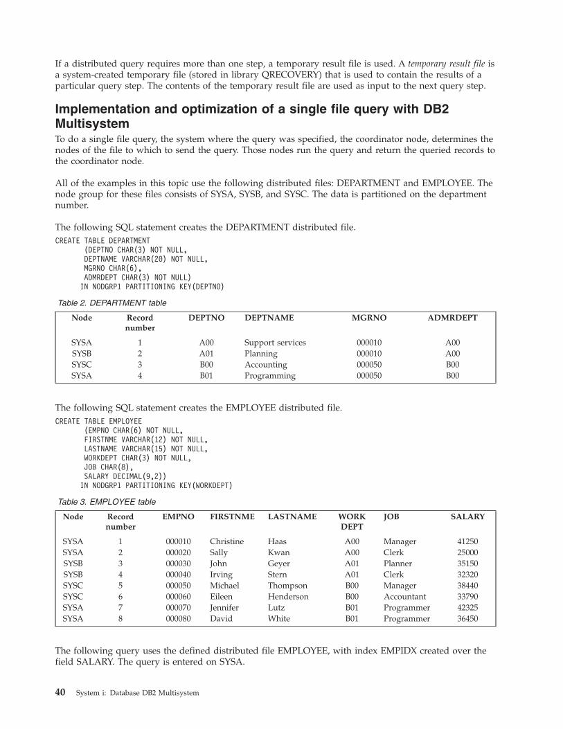
If a distributed query requires more than one step, a temporary result file is used. A temporary result file is
a system-created temporary file (stored in library QRECOVERY) that is used to contain the results of a
particular query step. The contents of the temporary result file are used as input to the next query step.
Implementation and optimization of a single file query with DB2
Multisystem
To do a single file query, the system where the query was specified, the coordinator node, determines the
nodes of the file to which to send the query. Those nodes run the query and return the queried records to
the coordinator node.
All of the examples in this topic use the following distributed files: DEPARTMENT and EMPLOYEE. The
node group for these files consists of SYSA, SYSB, and SYSC. The data is partitioned on the department
number.
The following SQL statement creates the DEPARTMENT distributed file.
CREATE TABLE DEPARTMENT
(DEPTNO CHAR(3) NOT NULL,
DEPTNAME VARCHAR(20) NOT NULL,
MGRNO CHAR(6),
ADMRDEPT CHAR(3) NOT NULL)
IN NODGRP1 PARTITIONING KEY(DEPTNO)
Table 2. DEPARTMENT table
Node Record
number
DEPTNO DEPTNAME MGRNO ADMRDEPT
SYSA 1 A00 Support services 000010 A00
SYSB 2 A01 Planning 000010 A00
SYSC 3 B00 Accounting 000050 B00
SYSA 4 B01 Programming 000050 B00
The following SQL statement creates the EMPLOYEE distributed file.
CREATE TABLE EMPLOYEE
(EMPNO CHAR(6) NOT NULL,
FIRSTNME VARCHAR(12) NOT NULL,
LASTNAME VARCHAR(15) NOT NULL,
WORKDEPT CHAR(3) NOT NULL,
JOB CHAR(8),
SALARY DECIMAL(9,2))
IN NODGRP1 PARTITIONING KEY(WORKDEPT)
Table 3. EMPLOYEE table
Node Record
number
EMPNO FIRSTNME LASTNAME WORK
DEPT
JOB SALARY
SYSA 1 000010 Christine Haas A00 Manager 41250
SYSA 2 000020 Sally Kwan A00 Clerk 25000
SYSB 3 000030 John Geyer A01 Planner 35150
SYSB 4 000040 Irving Stern A01 Clerk 32320
SYSC 5 000050 Michael Thompson B00 Manager 38440
SYSC 6 000060 Eileen Henderson B00 Accountant 33790
SYSA 7 000070 Jennifer Lutz B01 Programmer 42325
SYSA 8 000080 David White B01 Programmer 36450
The following query uses the defined distributed file EMPLOYEE, with index EMPIDX created over the
field SALARY. The query is entered on SYSA.
40 System i: Database DB2 Multisystem
SQL statement:
SELECT * FROM EMPLOYEE WHERE SALARY > 40000
OPNQRYF command:
OPNQRYF FILE((EMPLOYEE)) QRYSLT(’SALARY > 40000’)
In this case, SYSA sends the query to all the nodes of EMPLOYEE, including SYSA. Each node runs the
query and returns the records to SYSA. Because a distributed index exists on field SALARY of file
EMPLOYEE, optimization that is done on each node decides whether to use the index.
In the next example, the query is specified on SYSA, but the query is sent to a subset of the nodes where
the EMPLOYEE file exists. In this case, the query is run locally on SYSA only.
SQL statement:
SELECT * FROM EMPLOYEE WHERE WORKDEPT = ’A00’
OPNQRYF command:
OPNQRYF FILE((EMPLOYEE)) QRYSLT(’WORKDEPT = ’A00’)
The distributed query optimizer determines that there is an isolatable record selection, WORKDEPT =
’A00’, involving the partitioning key, WORKDEPT, for this query. The optimizer hashes the value ’A00’
and based on the hash value, finds the node at which all of the records satisfying this condition are
located. In this case, all of the records satisfying this condition are on SYSA, thus the query is sent only to
that node. Because the query originated on SYSA, the query is run locally on SYSA.
The following conditions subset the number of nodes at which a query runs:
v All fields of the partitioning key must be isolatable record selection
v All predicates must use the equal (=) operator
v All fields of the partitioning key must be compared to a literal
Note: For performance reasons, you should specify record selection predicates that match the partitioning
key in order to direct the query to a particular node. Record selection with scalar functions of
NODENAME, PARTITION, and NODENUMBER can also direct the query to specific nodes.
Implementation and optimization of record ordering with DB2
Multisystem
When ordering is specified on a query, the ordering criteria is sent along with the query, so that each
node can perform the ordering in parallel. Whether a final merge or a sort is performed on the
coordinator node is dependent on the type of query that you specify.
A merge of the ordered records received from each node is the most optimal. A merge occurs as the
records are received by the coordinator node. The main performance advantage that a merge has over a
sort is that the records can be returned without having to sort all of the records from every node.
A sort of the ordered records received from each node causes all of the records from each node to be
read, sorted, and written to a temporary result file before any records are returned.
A merge can occur if ordering is specified and no UNION and no final grouping are required. Otherwise,
for ordering queries, a final sort is performed on the coordinator node.
The allow copy data (ALWCPYDTA) parameter affects how each node of the distributed query processes
the ordering criteria. The ALWCPYDTA parameter is specified on the Open Query File (OPNQRYF) and
Start SQL (STRSQL) CL commands and also on the Create SQLxxx (CRTSQLxxx) precompiler commands:
DB2 Multisystem 41
v ALWCPYDTA(*OPTIMIZE) allows each node to choose to use either a sort or an index to implement
the ordering criteria. This option is the most optimal.
v For the OPNQRYF command and the query API (QQQQRY), ALWCPYDTA(*YES) or
ALWCPYDTA(*NO) enforces that each node use an index that exactly matches the specified ordering
fields. This is more restrictive than how the optimizer processes ordering for local files.
Implementation and optimization of the UNION and DISTINCT clauses
with DB2 Multisystem
If a unioned SELECT statement refers to a distributed file, the statement is processed as a distributed
query.
The processing of the statement can occur in parallel. However, the records from each unioned SELECT
are brought back to the coordinator node to perform the union operation. In this regard, the union
operators are processed serially.
If an ORDER BY clause is specified with a union query, all of the records from each node are received on
the coordinator node and are sorted before any records are returned.
When the DISTINCT clause is specified for a distributed query, adding an ORDER BY clause returns
records faster than if no ORDER BY clause was specified. DISTINCT with an ORDER BY allows each
node to order the records in parallel. A final merge on the coordinator node reads the ordered records
from each node, merges the records in the proper order, and eliminates duplicate records without having
to do a final sort.
When the DISTINCT clause is specified without an ORDER BY clause, all of the records from each node
are sent to the coordinator node where a sort is performed. Duplicate records are eliminated as the sorted
records are returned.
Processing of the DSTDTA and ALWCPYDTA parameters with DB2
Multisystem
The allow copy data (ALWCPYDTA) parameter can change the value specified for the distribute data
(DSTDTA) parameter of the Override Database File (OVRDBF) command.
If you specified to use live data (DSTDTA(*CURRENT)) on the override command, either of the following
items is true:
v A temporary copy is required and ALWCPYDTA(*YES) is specified
v A temporary copy is chosen for better performance and ALWCPYDTA(*OPTIMIZE) is specified
then DSTDTA is changed to DSTDTA(*BUFFERED).
If DSTDTA(*BUFFERED) is not acceptable to you and the query does not require a temporary copy, then
you need to specify ALWCPYDTA(*YES) to keep DSTDTA(*CURRENT) in effect.
Implementation and optimization of join operations with DB2
Multisystem
In addition to the performance considerations for nondistributed join queries, more performance
considerations exist for queries involving distributed files.
Joins can be performed only when the data is partition compatible. The distributed query optimizer
generates a plan that makes data partition compatible, which might involve moving data between nodes.
42 System i: Database DB2 Multisystem
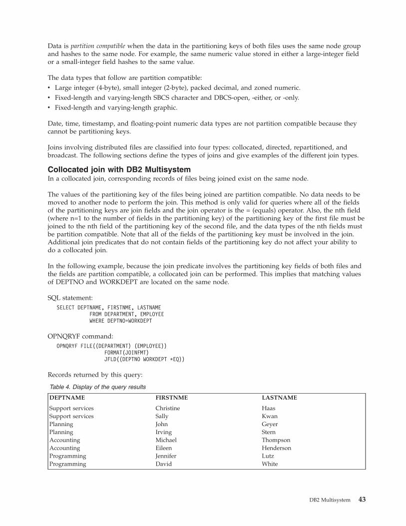
Data is partition compatible when the data in the partitioning keys of both files uses the same node group
and hashes to the same node. For example, the same numeric value stored in either a large-integer field
or a small-integer field hashes to the same value.
The data types that follow are partition compatible:
v Large integer (4-byte), small integer (2-byte), packed decimal, and zoned numeric.
v Fixed-length and varying-length SBCS character and DBCS-open, -either, or -only.
v Fixed-length and varying-length graphic.
Date, time, timestamp, and floating-point numeric data types are not partition compatible because they
cannot be partitioning keys.
Joins involving distributed files are classified into four types: collocated, directed, repartitioned, and
broadcast. The following sections define the types of joins and give examples of the different join types.
Collocated join with DB2 Multisystem
In a collocated join, corresponding records of files being joined exist on the same node.
The values of the partitioning key of the files being joined are partition compatible. No data needs to be
moved to another node to perform the join. This method is only valid for queries where all of the fields
of the partitioning keys are join fields and the join operator is the = (equals) operator. Also, the nth field
(where n=1 to the number of fields in the partitioning key) of the partitioning key of the first file must be
joined to the nth field of the partitioning key of the second file, and the data types of the nth fields must
be partition compatible. Note that all of the fields of the partitioning key must be involved in the join.
Additional join predicates that do not contain fields of the partitioning key do not affect your ability to
do a collocated join.
In the following example, because the join predicate involves the partitioning key fields of both files and
the fields are partition compatible, a collocated join can be performed. This implies that matching values
of DEPTNO and WORKDEPT are located on the same node.
SQL statement:
SELECT DEPTNAME, FIRSTNME, LASTNAME
FROM DEPARTMENT, EMPLOYEE
WHERE DEPTNO=WORKDEPT
OPNQRYF command:
OPNQRYF FILE((DEPARTMENT) (EMPLOYEE))
FORMAT(JOINFMT)
JFLD((DEPTNO WORKDEPT *EQ))
Records returned by this query:
Table 4. Display of the query results
DEPTNAME FIRSTNME LASTNAME
Support services Christine Haas
Support services Sally Kwan
Planning John Geyer
Planning Irving Stern
Accounting Michael Thompson
Accounting Eileen Henderson
Programming Jennifer Lutz
Programming David White
DB2 Multisystem 43
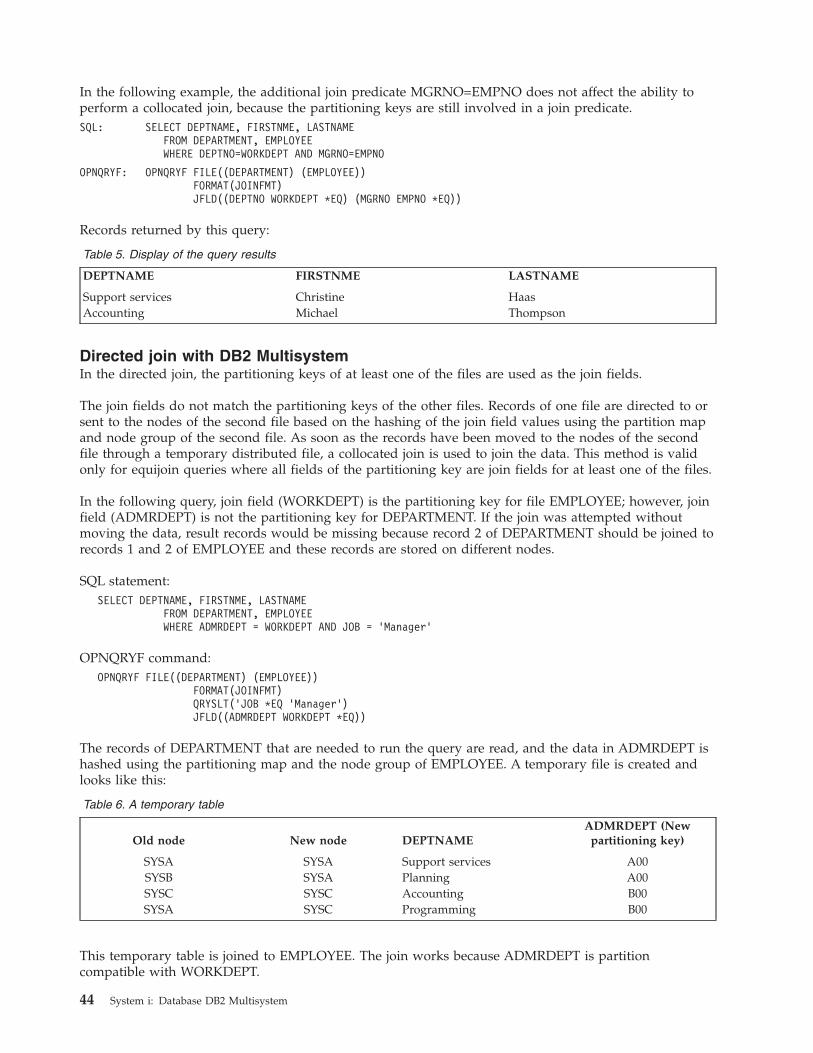
In the following example, the additional join predicate MGRNO=EMPNO does not affect the ability to
perform a collocated join, because the partitioning keys are still involved in a join predicate.
SQL: SELECT DEPTNAME, FIRSTNME, LASTNAME
FROM DEPARTMENT, EMPLOYEE
WHERE DEPTNO=WORKDEPT AND MGRNO=EMPNO
OPNQRYF: OPNQRYF FILE((DEPARTMENT) (EMPLOYEE))
FORMAT(JOINFMT)
JFLD((DEPTNO WORKDEPT *EQ) (MGRNO EMPNO *EQ))
Records returned by this query:
Table 5. Display of the query results
DEPTNAME FIRSTNME LASTNAME
Support services Christine Haas
Accounting Michael Thompson
Directed join with DB2 Multisystem
In the directed join, the partitioning keys of at least one of the files are used as the join fields.
The join fields do not match the partitioning keys of the other files. Records of one file are directed to or
sent to the nodes of the second file based on the hashing of the join field values using the partition map
and node group of the second file. As soon as the records have been moved to the nodes of the second
file through a temporary distributed file, a collocated join is used to join the data. This method is valid
only for equijoin queries where all fields of the partitioning key are join fields for at least one of the files.
In the following query, join field (WORKDEPT) is the partitioning key for file EMPLOYEE; however, join
field (ADMRDEPT) is not the partitioning key for DEPARTMENT. If the join was attempted without
moving the data, result records would be missing because record 2 of DEPARTMENT should be joined to
records 1 and 2 of EMPLOYEE and these records are stored on different nodes.
SQL statement:
SELECT DEPTNAME, FIRSTNME, LASTNAME
FROM DEPARTMENT, EMPLOYEE
WHERE ADMRDEPT = WORKDEPT AND JOB = ’Manager’
OPNQRYF command:
OPNQRYF FILE((DEPARTMENT) (EMPLOYEE))
FORMAT(JOINFMT)
QRYSLT(’JOB *EQ ’Manager’)
JFLD((ADMRDEPT WORKDEPT *EQ))
The records of DEPARTMENT that are needed to run the query are read, and the data in ADMRDEPT is
hashed using the partitioning map and the node group of EMPLOYEE. A temporary file is created and
looks like this:
Table 6. A temporary table
Old node New node DEPTNAME
ADMRDEPT (New
partitioning key)
SYSA SYSA Support services A00
SYSB SYSA Planning A00
SYSC SYSC Accounting B00
SYSA SYSC Programming B00
This temporary table is joined to EMPLOYEE. The join works because ADMRDEPT is partition
compatible with WORKDEPT.
44 System i: Database DB2 Multisystem
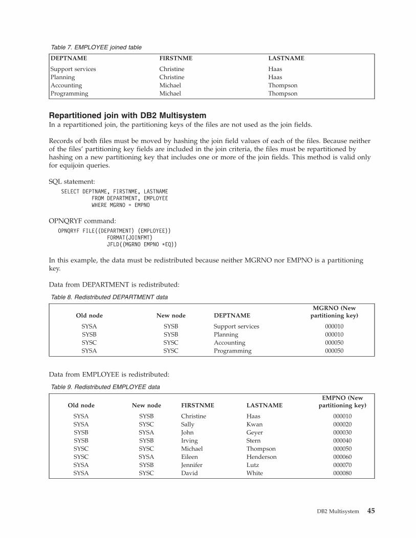
Table 7. EMPLOYEE joined table
DEPTNAME FIRSTNME LASTNAME
Support services Christine Haas
Planning Christine Haas
Accounting Michael Thompson
Programming Michael Thompson
Repartitioned join with DB2 Multisystem
In a repartitioned join, the partitioning keys of the files are not used as the join fields.
Records of both files must be moved by hashing the join field values of each of the files. Because neither
of the files’ partitioning key fields are included in the join criteria, the files must be repartitioned by
hashing on a new partitioning key that includes one or more of the join fields. This method is valid only
for equijoin queries.
SQL statement:
SELECT DEPTNAME, FIRSTNME, LASTNAME
FROM DEPARTMENT, EMPLOYEE
WHERE MGRNO = EMPNO
OPNQRYF command:
OPNQRYF FILE((DEPARTMENT) (EMPLOYEE))
FORMAT(JOINFMT)
JFLD((MGRNO EMPNO *EQ))
In this example, the data must be redistributed because neither MGRNO nor EMPNO is a partitioning
key.
Data from DEPARTMENT is redistributed:
Table 8. Redistributed DEPARTMENT data
Old node New node DEPTNAME
MGRNO (New
partitioning key)
SYSA SYSB Support services 000010
SYSB SYSB Planning 000010
SYSC SYSC Accounting 000050
SYSA SYSC Programming 000050
Data from EMPLOYEE is redistributed:
Table 9. Redistributed EMPLOYEE data
Old node New node FIRSTNME LASTNAME
EMPNO (New
partitioning key)
SYSA SYSB Christine Haas 000010
SYSA SYSC Sally Kwan 000020
SYSB SYSA John Geyer 000030
SYSB SYSB Irving Stern 000040
SYSC SYSC Michael Thompson 000050
SYSC SYSA Eileen Henderson 000060
SYSA SYSB Jennifer Lutz 000070
SYSA SYSC David White 000080
DB2 Multisystem 45
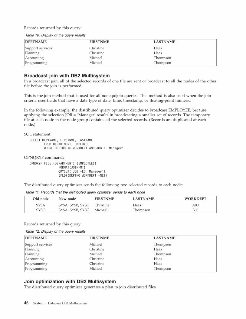
Records returned by this query:
Table 10. Display of the query results
DEPTNAME FIRSTNME LASTNAME
Support services Christine Haas
Planning Christine Haas
Accounting Michael Thompson
Programming Michael Thompson
Broadcast join with DB2 Multisystem
In a broadcast join, all of the selected records of one file are sent or broadcast to all the nodes of the other
file before the join is performed.
This is the join method that is used for all nonequijoin queries. This method is also used when the join
criteria uses fields that have a data type of date, time, timestamp, or floating-point numeric.
In the following example, the distributed query optimizer decides to broadcast EMPLOYEE, because
applying the selection JOB = ’Manager’ results in broadcasting a smaller set of records. The temporary
file at each node in the node group contains all the selected records. (Records are duplicated at each
node.)
SQL statement:
SELECT DEPTNAME, FIRSTNME, LASTNAME
FROM DEPARTMENT, EMPLOYEE
WHERE DEPTNO <> WORKDEPT AND JOB = ’Manager’
OPNQRYF command:
OPNQRYF FILE((DEPARTMENT) (EMPLOYEE))
FORMAT(JOINFMT)
QRYSLT(’JOB *EQ ’Manager’)
JFLD((DEPTNO WORKDEPT *NE))
The distributed query optimizer sends the following two selected records to each node:
Table 11. Records that the distributed query optimizer sends to each node
Old node New node FIRSTNME LASTNAME WORKDEPT
SYSA SYSA, SYSB, SYSC Christine Haas A00
SYSC SYSA, SYSB, SYSC Michael Thompson B00
Records returned by this query:
Table 12. Display of the query results
DEPTNAME FIRSTNME LASTNAME
Support services Michael Thompson
Planning Christine Haas
Planning Michael Thompson
Accounting Christine Haas
Programming Christine Haas
Programming Michael Thompson
Join optimization with DB2 Multisystem
The distributed query optimizer generates a plan to join distributed files.
46 System i: Database DB2 Multisystem
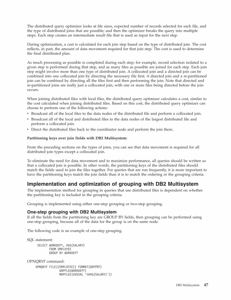
The distributed query optimizer looks at file sizes, expected number of records selected for each file, and
the type of distributed joins that are possible; and then the optimizer breaks the query into multiple
steps. Each step creates an intermediate result file that is used as input for the next step.
During optimization, a cost is calculated for each join step based on the type of distributed join. The cost
reflects, in part, the amount of data movement required for that join step. The cost is used to determine
the final distributed plan.
As much processing as possible is completed during each step; for example, record selection isolated to a
given step is performed during that step, and as many files as possible are joined for each step. Each join
step might involve more than one type of distributed join. A collocated join and a directed join can be
combined into one collocated join by directing the necessary file first. A directed join and a re-partitioned
join can be combined by directing all the files first and then performing the join. Note that directed and
re-partitioned joins are really just a collocated join, with one or more files being directed before the join
occurs.
When joining distributed files with local files, the distributed query optimizer calculates a cost, similar to
the cost calculated when joining distributed files. Based on this cost, the distributed query optimizer can
choose to perform one of the following actions:
v Broadcast all of the local files to the data nodes of the distributed file and perform a collocated join.
v Broadcast all of the local and distributed files to the data nodes of the largest distributed file and
perform a collocated join.
v Direct the distributed files back to the coordinator node and perform the join there.
Partitioning keys over join fields with DB2 Multisystem:
From the preceding sections on the types of joins, you can see that data movement is required for all
distributed join types except a collocated join.
To eliminate the need for data movement and to maximize performance, all queries should be written so
that a collocated join is possible. In other words, the partitioning keys of the distributed files should
match the fields used to join the files together. For queries that are run frequently, it is more important to
have the partitioning keys match the join fields than it is to match the ordering or the grouping criteria.
Implementation and optimization of grouping with DB2 Multisystem
The implementation method for grouping in queries that use distributed files is dependent on whether
the partitioning key is included in the grouping criteria.
Grouping is implemented using either one-step grouping or two-step grouping.
One-step grouping with DB2 Multisystem
If all the fields from the partitioning key are GROUP BY fields, then grouping can be performed using
one-step grouping, because all of the data for the group is on the same node.
The following code is an example of one-step grouping.
SQL statement:
SELECT WORKDEPT, AVG(SALARY)
FROM EMPLOYEE
GROUP BY WORKDEPT
OPNQRYF command:
OPNQRYF FILE((EMPLOYEE)) FORMAT(GRPFMT)
GRPFLD(WORKDEPT)
MAPFLD((AVGSAL ’%AVG(SALARY)’))
DB2 Multisystem 47
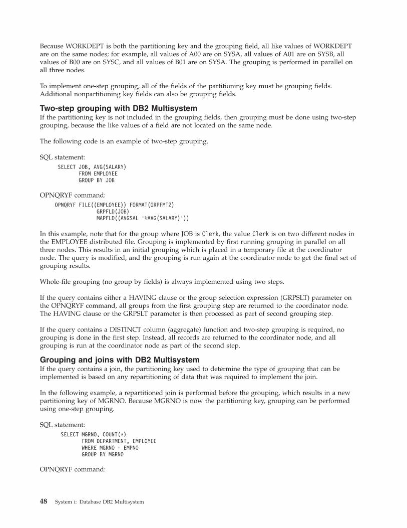
Because WORKDEPT is both the partitioning key and the grouping field, all like values of WORKDEPT
are on the same nodes; for example, all values of A00 are on SYSA, all values of A01 are on SYSB, all
values of B00 are on SYSC, and all values of B01 are on SYSA. The grouping is performed in parallel on
all three nodes.
To implement one-step grouping, all of the fields of the partitioning key must be grouping fields.
Additional nonpartitioning key fields can also be grouping fields.
Two-step grouping with DB2 Multisystem
If the partitioning key is not included in the grouping fields, then grouping must be done using two-step
grouping, because the like values of a field are not located on the same node.
The following code is an example of two-step grouping.
SQL statement:
SELECT JOB, AVG(SALARY)
FROM EMPLOYEE
GROUP BY JOB
OPNQRYF command:
OPNQRYF FILE((EMPLOYEE)) FORMAT(GRPFMT2)
GRPFLD(JOB)
MAPFLD((AVGSAL ’%AVG(SALARY)’))
In this example, note that for the group where JOB is Clerk, the value Clerk is on two different nodes in
the EMPLOYEE distributed file. Grouping is implemented by first running grouping in parallel on all
three nodes. This results in an initial grouping which is placed in a temporary file at the coordinator
node. The query is modified, and the grouping is run again at the coordinator node to get the final set of
grouping results.
Whole-file grouping (no group by fields) is always implemented using two steps.
If the query contains either a HAVING clause or the group selection expression (GRPSLT) parameter on
the OPNQRYF command, all groups from the first grouping step are returned to the coordinator node.
The HAVING clause or the GRPSLT parameter is then processed as part of second grouping step.
If the query contains a DISTINCT column (aggregate) function and two-step grouping is required, no
grouping is done in the first step. Instead, all records are returned to the coordinator node, and all
grouping is run at the coordinator node as part of the second step.
Grouping and joins with DB2 Multisystem
If the query contains a join, the partitioning key used to determine the type of grouping that can be
implemented is based on any repartitioning of data that was required to implement the join.
In the following example, a repartitioned join is performed before the grouping, which results in a new
partitioning key of MGRNO. Because MGRNO is now the partitioning key, grouping can be performed
using one-step grouping.
SQL statement:
SELECT MGRNO, COUNT(*)
FROM DEPARTMENT, EMPLOYEE
WHERE MGRNO = EMPNO
GROUP BY MGRNO
OPNQRYF command:
48 System i: Database DB2 Multisystem
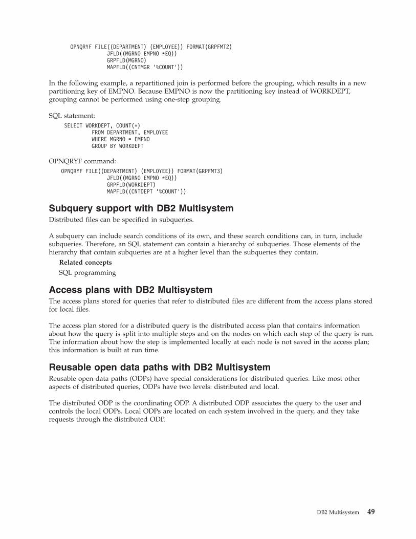
OPNQRYF FILE((DEPARTMENT) (EMPLOYEE)) FORMAT(GRPFMT2)
JFLD((MGRNO EMPNO *EQ))
GRPFLD(MGRNO)
MAPFLD((CNTMGR ’%COUNT’))
In the following example, a repartitioned join is performed before the grouping, which results in a new
partitioning key of EMPNO. Because EMPNO is now the partitioning key instead of WORKDEPT,
grouping cannot be performed using one-step grouping.
SQL statement:
SELECT WORKDEPT, COUNT(*)
FROM DEPARTMENT, EMPLOYEE
WHERE MGRNO = EMPNO
GROUP BY WORKDEPT
OPNQRYF command:
OPNQRYF FILE((DEPARTMENT) (EMPLOYEE)) FORMAT(GRPFMT3)
JFLD((MGRNO EMPNO *EQ))
GRPFLD(WORKDEPT)
MAPFLD((CNTDEPT ’%COUNT’))
Subquery support with DB2 Multisystem
Distributed files can be specified in subqueries.
A subquery can include search conditions of its own, and these search conditions can, in turn, include
subqueries. Therefore, an SQL statement can contain a hierarchy of subqueries. Those elements of the
hierarchy that contain subqueries are at a higher level than the subqueries they contain.
Related concepts
SQL programming
Access plans with DB2 Multisystem
The access plans stored for queries that refer to distributed files are different from the access plans stored
for local files.
The access plan stored for a distributed query is the distributed access plan that contains information
about how the query is split into multiple steps and on the nodes on which each step of the query is run.
The information about how the step is implemented locally at each node is not saved in the access plan;
this information is built at run time.
Reusable open data paths with DB2 Multisystem
Reusable open data paths (ODPs) have special considerations for distributed queries. Like most other
aspects of distributed queries, ODPs have two levels: distributed and local.
The distributed ODP is the coordinating ODP. A distributed ODP associates the query to the user and
controls the local ODPs. Local ODPs are located on each system involved in the query, and they take
requests through the distributed ODP.
DB2 Multisystem 49
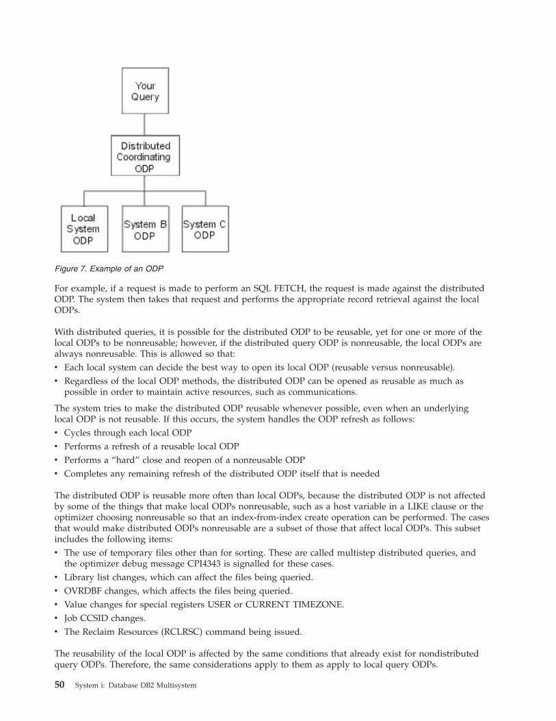
For example, if a request is made to perform an SQL FETCH, the request is made against the distributed
ODP. The system then takes that request and performs the appropriate record retrieval against the local
ODPs.
With distributed queries, it is possible for the distributed ODP to be reusable, yet for one or more of the
local ODPs to be nonreusable; however, if the distributed query ODP is nonreusable, the local ODPs are
always nonreusable. This is allowed so that:
v Each local system can decide the best way to open its local ODP (reusable versus nonreusable).
v Regardless of the local ODP methods, the distributed ODP can be opened as reusable as much as
possible in order to maintain active resources, such as communications.
The system tries to make the distributed ODP reusable whenever possible, even when an underlying
local ODP is not reusable. If this occurs, the system handles the ODP refresh as follows:
v Cycles through each local ODP
v Performs a refresh of a reusable local ODP
v Performs a “hard” close and reopen of a nonreusable ODP
v Completes any remaining refresh of the distributed ODP itself that is needed
The distributed ODP is reusable more often than local ODPs, because the distributed ODP is not affected
by some of the things that make local ODPs nonreusable, such as a host variable in a LIKE clause or the
optimizer choosing nonreusable so that an index-from-index create operation can be performed. The cases
that would make distributed ODPs nonreusable are a subset of those that affect local ODPs. This subset
includes the following items:
v The use of temporary files other than for sorting. These are called multistep distributed queries, and
the optimizer debug message CPI4343 is signalled for these cases.
v Library list changes, which can affect the files being queried.
v OVRDBF changes, which affects the files being queried.
v Value changes for special registers USER or CURRENT TIMEZONE.
v Job CCSID changes.
v The Reclaim Resources (RCLRSC) command being issued.
The reusability of the local ODP is affected by the same conditions that already exist for nondistributed
query ODPs. Therefore, the same considerations apply to them as apply to local query ODPs.
Figure 7. Example of an ODP
50 System i: Database DB2 Multisystem
Temporary result writer with DB2 Multisystem
Temporary result writers are system-initiated jobs that are always active.
On the system, temporary result writers are paired jobs called QQQTEMP1 and QQQTEMP2. Temporary
result writers handle requests from jobs that are running queries. These requests consist of a query (of the
query step) to run and the name of a system temporary file to fill from the results of the query. The
temporary result writer processes the request and fills the temporary file. This intermediate temporary
file is then used by the requesting job to complete the original query.
The following example shows a query that requires a temporary result writer and the steps needed to
process the query.
SQL statement:
SELECT COUNT(*)
FROM DEPARTMENT a, EMPLOYEE b
WHERE a.ADMRDEPT = b.WORKDEPT
AND b.JOB = ’Manager’
OPNQRYF command:
OPNQRYF FILE((DEPARTMENT) (EMPLOYEE))
FORMAT(FMTFILE)
MAPFLD((CNTFLD ’%COUNT’))
JFLD((1/ADMRDEPT 2/WORKDEPT))
QRYSLT(’2/JOB = ’Manager’)
WORKDEPT is the partitioning key for EMPLOYEE, but ADMRDEPT is not the partitioning key for
DEPARTMENT. Because the query must be processed in two steps, the optimizer splits the query into the
following steps:
INSERT INTO SYS_TEMP_FILE
SELECT a.DEPTNAME, a.ADMRDEPT
FROM DEPARTMENT a
and
SELECT COUNT(*) FROM SYS_TEMP_FILE x, EMPLOYEE b
WHERE x.ADMRDEPT = b.WORKDEPT AND b.JOB = ’Manager’
If a temporary result writer is allowed for the job (controlled by the Change Query Attributes
(CHGQRYA) options), the optimizer:
1. Creates the temporary file (SYS_TEMP_FILE) into library QRECOVERY.
2. Sends the request that populates SYS_TEMP_FILE to the temporary result writer.
3. Continues to finish opening the final query (while the temporary result writer is filling the temporary
file).
4. After the final query is opened, waits until the temporary result writer has finished filling the
temporary file before returning control to its caller. Related concepts
“Changes to the Change Query Attributes command with DB2 Multisystem” on page 54The Change Query Attributes command has two parameters that are applicable to distributed queries.
Temporary result writer job: Advantages with DB2 Multisystem
The advantage of using a temporary result writer job in processing a request is that the temporary result
writer can process its request at the same time (in parallel) that the main job is processing another step of
the query.
Performance advantages of using a temporary result writer are as follows:
DB2 Multisystem 51

v The temporary result writer can use full symmetric multiprocessing (SMP) parallel support in
completing its query step, while the main job can continue with more complex steps that do not lend
themselves as easily to parallel processing (such as query optimization, index analysis, and so on).
v Because distributed file processing requires communications interaction, a considerable amount of time
typically spent waiting for sending and receiving can be offloaded to the temporary result writer,
which leaves the main job to do other work.
Temporary result writer job: Disadvantages with DB2 Multisystem
The temporary result writer also has disadvantages that must be considered when you determine its
usefulness for queries.
The disadvantages are as follows:
v The temporary result writer is a separate job. Consequently, it can encounter conflicts with the main
job. Here are some examples:
– The main job might have the file locked to itself. In this case, the temporary result writer cannot
access the files and cannot complete its query step.
– The main job might have created the distributed file under commitment control and has not yet
committed the create. In this case, the temporary result writer cannot access the file.v The temporary result writer might encounter a situation that it cannot handle in the same way as the
main job. For example, if an inquiry message is signalled, the temporary result writer might cancel,
whereas the main job can choose to ignore the message and continue on.
v Temporary result writers are shared by all jobs on the system. If several jobs have requests to the
temporary result writers, the requests queue up while the writers attempt to process them.
Note: The system is shipped with three, active temporary result writer job pairs.
v Attempting to analyze a query (through debug messages, for example) can be complicated if a
temporary result writer is involved (because a step of the query is run in a separate job).
Note: The system does not allow the temporary result writer to be used for queries running under
commitment control *CS or *ALL. This is because the main job might have records locked in the
file, which can cause the temporary result writer to be locked out of these records and not be able
to finish.
Control of the temporary result writer with DB2 Multisystem
By default, queries do not use the temporary result writer. Temporary result writer usage, however, can
be enabled by using the Change Query Attributes (CHGQRYA) command.
The asynchronous job usage (ASYNCJ) parameter on the CHGQRYA command is used to control the
usage of the temporary result writer. The ASYNCJ parameter has the following applicable options:
v *DIST or *ANY allows the temporary result writer jobs to be used for queries involving distributed
files.
v *LOCAL or *NONE prevents the temporary result writer from being used for queries of distributed
files.
Optimizer messages with DB2 Multisystem
The i5/OS distributed query optimizer provides you with information messages on the current query
processing when the job is in debug mode.
These messages, which show how the distributed query is processed, are in addition to the existing
optimizer messages. These messages appear for the Open Query File (OPNQRYF) command, DB2 UDB
Query Manager and SQL Development Kit, interactive SQL, embedded SQL, and in any high-level
language (HLL). Every message appears in the job log; you only need to put your job into debug mode.
52 System i: Database DB2 Multisystem
You can evaluate the performance of your distributed query by using the informational messages put in
the job log by the database manager. The database manager can send any of the following distributed
messages or existing optimizer messages when appropriate. The ampersand variables (&1, &X) are
replacement variables that contain either an object name or another substitution value when the message
appears in the job log:
v CPI4341 Performing distributed query.
v CPI4342 Performing distributed join for query.
v CPI4343 Optimizer debug messages for distributed query step &1 of &2.
v CPI4345 Temporary distributed result file &4 built for query.
These messages provide feedback on how a distributed query is run, and, in some cases, indicate the
improvements that can be made to help the query run faster. The causes and user responses for the
following messages are paraphrased here. The actual message help is more complete and needs to be
used when you try to determine the meaning and responses for each message.
CPI4341
Performing distributed query.
This message indicates that a single distributed file was queried and was not processed in
multiple steps. This message lists the nodes of the file where the query was run.
CPI4342
Performing distributed join for query.
This message indicates that a distributed join occurred. This message also lists the nodes where
the join was run as well as the files that were joined together.
CPI4343
Optimizer debug messages for distributed query step &1 of &2.
This message indicates that a distributed query was processed in multiple steps and lists the
current step number. Following this message are all the optimizer messages for that step.
CPI4345
Temporary distributed result file &4 built for query.
This message indicates that a temporary distributed result file was created and lists a reason code
as to why the temporary file was required. This message also shows the partitioning key that was
used to create the file and the nodes that the temporary file was created on.
The following example shows you how to look at the distributed optimizer messages that are generated
to determine how the distributed query is processed. The example uses the distributed files, EMPLOYEE
and DEPARTMENT.
SQL: SELECT A.EMPNO, B.MGRNO, C.MGRNO, D.EMPNO
FROM EMPLOYEE A, DEPARTMENT B, DEPARTMENT C, EMPLOYEE D
WHERE A.EMPNO=B.MGRNO
AND B.ADMRDEPT=C.DEPTNO
AND C.DEPTNO=D.WORKDEPT
OPNQRYF: OPNQRYF FILE((EMPLOYEE) (DEPARTMENT) (DEPARTMENT) (EMPLOYEE))
FORMAT(JFMT)
JFLD((1/EMNO 2/MGRNO *EQ)
(2/ADMRDEPT 3/DEPTNO)
(3/DEPTNO 4/WORKDEPT))
The following list of distributed optimizer messages is generated:
v CPI4343 Optimizer debug messages for distributed query step &1 of &4 follow:
– CPI4345 Temporary distributed result file *QQTDF0001 built for query.
File B was directed into temporary file *QQTDF0001.
DB2 Multisystem 53
v CPI4343 Optimizer debug messages for distributed query step &2 of &4 follow:
– CPI4342 Performing distributed join for query.
Files B, C and *QQTDF0001 were joined. This was a combination of a collocated join (between files
B and C) and a directed join (with file *QQTDF0001).
– CPI4345 Temporary distributed result file *QQTDF0002 built for query.
Temporary distributed file *QQTDF0002 was created to contain the result of joining files B, C and
*QQTDF0001. This file was directed.v CPI4343 Optimizer debug messages for distributed query step &3 of &4 follow:
– CPI4345 Temporary distributed result file *QQTDF0003 built for query.
File A was directed into temporary file *QQTDF0003.v CPI4343 Optimizer debug messages for distributed query step &4 of &4 follow:
– CPI4342 Performing distributed join for query.
Files *QQTDF0002 and *QQTDF0003 were joined. This was a repartitioned join, because both files
were directed before the join occurred.
Additional tools that you might want to use when tuning queries for performance include the CL
commands Print SQL Information (PRTSQLINF), which applies to SQL programs and packages, and
Change Query Attributes (CHGQRYA).
Changes to the Change Query Attributes command with DB2
Multisystem
The Change Query Attributes command has two parameters that are applicable to distributed queries.
The two parameters are: ASYNCJ (asynchronous job usage) and APYRMT (apply remote).
Note: Unlike other parameters, ASYNCJ and APYRMT have no system values. If a value other than the
default is necessary, the value must be changed for each job.
Related reference
“Temporary result writer with DB2 Multisystem” on page 51Temporary result writers are system-initiated jobs that are always active.
Asynchronous job usage parameter with DB2 Multisystem
You can use the asynchronous job usage (ASYNCJ) parameter to control the usage of the temporary result
writer.
The ASYNCJ parameter has the following options:
v *ANY—allows the temporary result writer jobs to be used for database queries involving distributed
files.
v *DIST—allows the temporary result writer jobs to be used for database queries involving distributed
files.
v *LOCAL—allows the temporary result writer jobs to be used for queries of local files only. Although
this option is allowed, currently there is no system support for using temporary result writers for local
query processing. *LOCAL was added to disable the temporary result writer for distributed queries,
yet still allow communications to be performed asynchronously.
v *NONE—never use the temporary result writer. In addition, when distributed processing is performed,
communications are performed synchronously. This can be very useful when analyzing queries,
because it allows query debug messages from remote systems to be returned to the local system.
The following example shows you how to disable asynchronous job usage for distributed file processing:
CHGQRYA ASYNCJ(*LOCAL)
54 System i: Database DB2 Multisystem
This command prevents asynchronous jobs from being used for queries involving distributed files.
The following example shows you how to completely disable asynchronous job usage:
CHGQRYA ASYNCJ(*NONE)
This command prevents asynchronous jobs from being used for any queries. In addition, for queries
involving distributed files, communications to remote systems are done in a synchronous fashion.
The following example shows you how to use the CHGQRYA command in combination with the Start
Debug (STRDBG) command to analyze a distributed query:
STRDBG UPDPROD(*YES)
CHGQRYA ASYNCJ(*NONE)
STRSQL
SELECT COUNT(*) FROM EMPLOYEE A
The following debug messages are put into the job log:
Current connection is to relational database SYSA.
DDM job started.
Optimizer debug messages for distributed query step 1 of 2 follow:
Temporary distributed result file *QQTDF0001 built for query.
Following messages created on target system SYSB.
Arrival sequence access was used for file EMPLOYEE.
Arrival sequence access was used for file EMPLOYEE.
Optimizer debug messages for distributed query step 2 of 2 follow:
Arrival sequence access was used for file EMPLOYEE.
ODP created.
Blocking used for query.
Apply remote parameter with DB2 Multisystem
You can use the apply remote (APYRMT) parameter to specify whether the other CHGQRYA options
should be applied to the associated remote system jobs that are used in the processing of the distributed
query requests.
The APYRMT parameter has the following options:
v *YES—apply the CHGQRYA options to remote jobs. This requires that the remote job have authority to
use the CHGQRYA command. Otherwise, an error is signalled to the remote job.
v *NO—apply the CHGQRYA options only locally.
Note: If the query attribute of the APYRMT parameter is *YES and the QAQQINI file has *NO for
applying remote system jobs, the query attribute of the APYRMT parameter will be overridden by
*NO.
The following example prevents the CHGQRYA options from being applied remotely:
CHGQRYA DEGREE(*NONE) APYRMT(*NO)
In this case, symmetric multiprocessing (SMP) parallel support is prevented on the coordinator node, but
the remote systems are allowed to choose their own parallel degree.
In addition to these parameters, you should be aware of how the parameter Query Time Limit
(QRYTIMLMT) works. The time limit specified on the parameter is applied to each step (local and
remote) of the distributed query; it is not applied to the entire query. Therefore, it is possible for one
query step to encounter the time limit; whereas, another step can continue without problems. While the
time limit option can be quite useful, it should be used with caution on distributed queries.
Summary of performance considerations
You should consider these performance factors when developing queries that use distributed files.
DB2 Multisystem 55
|||
1. For the OPNQRYF command and the query API (QQQQRY), specifying ALWCPYDTA(*OPTIMIZE)
allows each node to choose an index or a sort to satisfy the ordering specified.
2. For the OPNQRYF command and the query API (QQQQRY), specifying ALWCPYDTA(*YES) or
ALWCPYDTA(*NO) enforces that each node use an index that exactly matches the specified ordering
fields. This is more restrictive than the way the optimizer processes ordering for nondistributed files.
3. Adding an ORDER BY clause to a DISTINCT select can return records faster by not requiring a final
sort on the requesting system.
4. Including all of the fields of the partitioning key in the grouping fields generally results in one-step
grouping, which performs better than two-step grouping.
5. Including all of the fields of the partitioning key in the join criteria generally results in a collocated
distributed join.
6. Including all of the fields of the partitioning key in isolatable, equal record selection generally results
in the query being processed on only one node.
7. Including any of the following scalar functions in isolatable, equal record selection generally results in
the query being processed on only one node:
v NODENAME
v NODENUMBER
v PARTITION
Related information for DB2 Multisystem
Listed here are the information center topics that relate to the DB2 Multisystem topic.
v Application programming interfaces provides information for the experienced programmer on how to
use the application programming interfaces (APIs) for some operating system functions.
v Backup, Recovery, and Media Services (BRMS) provides information about setting up and managing:
– Journaling, access path protection, and commitment control
– User auxiliary storage pools (ASPs)
– Disk protection (device parity, mirrored, and checksum)
This topic collection also provides performance information about backup media and save/restore
operations. It also includes advanced backup and recovery topics, such as using save-while-active
support, saving and restoring to a different release, and programming tips and techniques.
v Control language provides an overview of all the CL commands and describes the syntax rules needed
to code them.
v Database programming provides a detailed discussion of the i5/OS database organization, including
information about how to create, describe, and update database files on the system.
v Distributed database programming provides information about preparing and managing a System i
product in a distributed relational database using the Distributed Relational Database Architecture
(DRDA). It describes planning, setting up, programming, administering, and operating a distributed
relational database on more than one system in a like-system environment.
v Install, upgrade, or delete i5/OS and related software includes planning information and step-by-step
instructions for procedures to install the operating system and licensed programs.
v OptiConnect describes OptiConnect support, which can connect multiple systems using a fiber optic
cable. OptiConnect allows you to access intersystem databases more quickly and enables you to offload
work to another system. Additional topics include configuration, installation, and operation
information.
v SQL programming provides information about how to use DB2 for the DB2 UDB Query Manager and
SQL Development Kit licensed program. This topic collection shows how to access data in a database
library and how to prepare, run, and test an application program that contains embedded SQL
statements. The topic collection also contains examples of SQL statements and a description of the
interactive SQL function, and describes common concepts and rules for using SQL statements in
56 System i: Database DB2 Multisystem
COBOL, ILE COBOL, PL/I, ILE C, FORTRAN/400, RPG, ILE RPG, and REXX. SQL programming and
Database programming also provide information about DB2 UDB Symmetric Multiprocessing.
v SQL reference provides information about how to use DB2 SQL statements and gives details about the
proper use of the statements. Examples of statements include syntax diagrams, parameters, and
definitions. A list of SQL limitations and a description of the SQL communication area (SQLCA) and
SQL descriptor area (SQLDA) are also provided.
Code license and disclaimer information
IBM grants you a nonexclusive copyright license to use all programming code examples from which you
can generate similar function tailored to your own specific needs.
SUBJECT TO ANY STATUTORY WARRANTIES WHICH CANNOT BE EXCLUDED, IBM, ITS
PROGRAM DEVELOPERS AND SUPPLIERS MAKE NO WARRANTIES OR CONDITIONS EITHER
EXPRESS OR IMPLIED, INCLUDING BUT NOT LIMITED TO, THE IMPLIED WARRANTIES OR
CONDITIONS OF MERCHANTABILITY, FITNESS FOR A PARTICULAR PURPOSE, AND
NON-INFRINGEMENT, REGARDING THE PROGRAM OR TECHNICAL SUPPORT, IF ANY.
UNDER NO CIRCUMSTANCES IS IBM, ITS PROGRAM DEVELOPERS OR SUPPLIERS LIABLE FOR
ANY OF THE FOLLOWING, EVEN IF INFORMED OF THEIR POSSIBILITY:
1. LOSS OF, OR DAMAGE TO, DATA;
2. DIRECT, SPECIAL, INCIDENTAL, OR INDIRECT DAMAGES, OR FOR ANY ECONOMIC
CONSEQUENTIAL DAMAGES; OR
3. LOST PROFITS, BUSINESS, REVENUE, GOODWILL, OR ANTICIPATED SAVINGS.
SOME JURISDICTIONS DO NOT ALLOW THE EXCLUSION OR LIMITATION OF DIRECT,
INCIDENTAL, OR CONSEQUENTIAL DAMAGES, SO SOME OR ALL OF THE ABOVE LIMITATIONS
OR EXCLUSIONS MAY NOT APPLY TO YOU.
DB2 Multisystem 57
|||||
||
|
||
|
|||

58 System i: Database DB2 Multisystem
Appendix. Notices
This information was developed for products and services offered in the U.S.A.
IBM may not offer the products, services, or features discussed in this document in other countries.
Consult your local IBM representative for information on the products and services currently available in
your area. Any reference to an IBM product, program, or service is not intended to state or imply that
only that IBM product, program, or service may be used. Any functionally equivalent product, program,
or service that does not infringe any IBM intellectual property right may be used instead. However, it is
the user’s responsibility to evaluate and verify the operation of any non-IBM product, program, or
service.
IBM may have patents or pending patent applications covering subject matter described in this
document. The furnishing of this document does not grant you any license to these patents. You can send
license inquiries, in writing, to:
IBM Director of Licensing
IBM Corporation
North Castle Drive
Armonk, NY 10504-1785
U.S.A.
For license inquiries regarding double-byte (DBCS) information, contact the IBM Intellectual Property
Department in your country or send inquiries, in writing, to:
IBM World Trade Asia Corporation
Licensing
2-31 Roppongi 3-chome, Minato-ku
Tokyo 106-0032, Japan
The following paragraph does not apply to the United Kingdom or any other country where such
provisions are inconsistent with local law: INTERNATIONAL BUSINESS MACHINES CORPORATION
PROVIDES THIS PUBLICATION “AS IS” WITHOUT WARRANTY OF ANY KIND, EITHER EXPRESS
OR IMPLIED, INCLUDING, BUT NOT LIMITED TO, THE IMPLIED WARRANTIES OF
NON-INFRINGEMENT, MERCHANTABILITY OR FITNESS FOR A PARTICULAR PURPOSE. Some
states do not allow disclaimer of express or implied warranties in certain transactions, therefore, this
statement may not apply to you.
This information could include technical inaccuracies or typographical errors. Changes are periodically
made to the information herein; these changes will be incorporated in new editions of the publication.
IBM may make improvements and/or changes in the product(s) and/or the program(s) described in this
publication at any time without notice.
Any references in this information to non-IBM Web sites are provided for convenience only and do not in
any manner serve as an endorsement of those Web sites. The materials at those Web sites are not part of
the materials for this IBM product and use of those Web sites is at your own risk.
IBM may use or distribute any of the information you supply in any way it believes appropriate without
incurring any obligation to you.
Licensees of this program who wish to have information about it for the purpose of enabling: (i) the
exchange of information between independently created programs and other programs (including this
one) and (ii) the mutual use of the information which has been exchanged, should contact:
IBM Corporation
© Copyright IBM Corp. 1998, 2006 59
Software Interoperability Coordinator, Department YBWA
3605 Highway 52 N
Rochester, MN 55901
U.S.A.
Such information may be available, subject to appropriate terms and conditions, including in some cases,
payment of a fee.
The licensed program described in this information and all licensed material available for it are provided
by IBM under terms of the IBM Customer Agreement, IBM International Program License Agreement,
IBM License Agreement for Machine Code, or any equivalent agreement between us.
Any performance data contained herein was determined in a controlled environment. Therefore, the
results obtained in other operating environments may vary significantly. Some measurements may have
been made on development-level systems and there is no guarantee that these measurements will be the
same on generally available systems. Furthermore, some measurements may have been estimated through
extrapolation. Actual results may vary. Users of this document should verify the applicable data for their
specific environment.
Information concerning non-IBM products was obtained from the suppliers of those products, their
published announcements or other publicly available sources. IBM has not tested those products and
cannot confirm the accuracy of performance, compatibility or any other claims related to non-IBM
products. Questions on the capabilities of non-IBM products should be addressed to the suppliers of
those products.
All statements regarding IBM’s future direction or intent are subject to change or withdrawal without
notice, and represent goals and objectives only.
This information contains examples of data and reports used in daily business operations. To illustrate
them as completely as possible, the examples include the names of individuals, companies, brands, and
products. All of these names are fictitious and any similarity to the names and addresses used by an
actual business enterprise is entirely coincidental.
COPYRIGHT LICENSE:
This information contains sample application programs in source language, which illustrate programming
techniques on various operating platforms. You may copy, modify, and distribute these sample programs
in any form without payment to IBM, for the purposes of developing, using, marketing or distributing
application programs conforming to the application programming interface for the operating platform for
which the sample programs are written. These examples have not been thoroughly tested under all
conditions. IBM, therefore, cannot guarantee or imply reliability, serviceability, or function of these
programs.
Each copy or any portion of these sample programs or any derivative work, must include a copyright
notice as follows:
© (your company name) (year). Portions of this code are derived from IBM Corp. Sample Programs. ©
Copyright IBM Corp. _enter the year or years_. All rights reserved.
If you are viewing this information softcopy, the photographs and color illustrations may not appear.
Programming Interface Information
This DB2 Multisystem publication documents intended Programming Interfaces that allow the customer
to write programs to obtain the services of IBM i5/OS.
60 System i: Database DB2 Multisystem
|||
Trademarks
The following terms are trademarks of International Business Machines Corporation in the United States,
other countries, or both:
DB2
DB2 Universal Database
Distributed Relational Database Architecture
DRDA
i5/OS
IBM (logo)
iSeries
System i
Other company, product, and service names may be trademarks or service marks of others.
Terms and conditions
Permissions for the use of these publications is granted subject to the following terms and conditions.
Personal Use: You may reproduce these publications for your personal, noncommercial use provided that
all proprietary notices are preserved. You may not distribute, display or make derivative works of these
publications, or any portion thereof, without the express consent of IBM.
Commercial Use: You may reproduce, distribute and display these publications solely within your
enterprise provided that all proprietary notices are preserved. You may not make derivative works of
these publications, or reproduce, distribute or display these publications or any portion thereof outside
your enterprise, without the express consent of IBM.
Except as expressly granted in this permission, no other permissions, licenses or rights are granted, either
express or implied, to the publications or any information, data, software or other intellectual property
contained therein.
IBM reserves the right to withdraw the permissions granted herein whenever, in its discretion, the use of
the publications is detrimental to its interest or, as determined by IBM, the above instructions are not
being properly followed.
You may not download, export or re-export this information except in full compliance with all applicable
laws and regulations, including all United States export laws and regulations.
IBM MAKES NO GUARANTEE ABOUT THE CONTENT OF THESE PUBLICATIONS. THE
PUBLICATIONS ARE PROVIDED ″AS-IS″ AND WITHOUT WARRANTY OF ANY KIND, EITHER
EXPRESSED OR IMPLIED, INCLUDING BUT NOT LIMITED TO IMPLIED WARRANTIES OF
MERCHANTABILITY, NON-INFRINGEMENT, AND FITNESS FOR A PARTICULAR PURPOSE.
Appendix. Notices 61
||||||||

62 System i: Database DB2 Multisystem


����
Printed in USA