Embed Size (px)
Citation preview

i
SYSTEM IDENTIFICATION AND
CONTROL OF MAGNETIC BEARING SYSTEMS
by
Fitriah Abdul Somad
A thesis submitted in fulfillment of the requirement for the degree of
Master of Engineering
(by Research)
2007
School of Electrical Engineering Victoria University
ii
ABSTRACT This thesis presents investigations aimed at obtaining a system model for the
stabilisation of an Active Magnetic Bearing (AMB) System. Furthermore, the study
reported here set out to design both conventional and advanced controllers based on the
system model.
This research report demonstrates that the literature on AMBs shows that AMBs are
making their mark in the industry; they are increasingly being used in applications
including jet engines, compressors, pumps and flywheel systems. In this study, it has
also been observed that the basic design of AMBs is an arrangement of electromagnets
placed equidistant in a ring round a rotor. The point of departure for this study is that
AMBs are highly nonlinear and inherently unstable. Hence, the need for an automatic
control to keep the system stabilized.
The first step of the research was to determine the transfer function of the MBC 500
magnetic bearing system both analytically and experimentally. An analytical model has
been derived based on principle of physics. As the AMB system under analysis is
inherently unstable, it was necessary to identify the model using a closed-loop system
identification. Frequency response data has been collected using the two-step closed-
loop system identification. As there are resonant modes in the MBC 500 magnetic
bearing system, the system identification approach has identified the corresponding
resonant frequencies. Subsequent to obtaining the model, a conventional controller was
designed to stabilise the AMB system. Two notch filters were designed to deal with the
magnitude and phase fluctuations around the two dominant resonant frequencies. The

iii
designed conventional controller and notch filters have been implemented using
MATLAB, SIMULINK and dSPACE DS1102 digital signal processing (DSP) card.
Both the step response and robustness tests have demonstrated the effectiveness of the
conventional controller and notch filters designed.
A significant conclusion has been drawn when designing the conventional controller. It
was found that a controller that had a large positive phase angle had a negative effect on
the system. This finding was very significant because it restricted the controller
specifications and yielded an optimum lead angle for the conventional controller.
The advanced PD-like Fuzzy Logic Controller (FLC) has also been designed for AMB
system stabilisation. The designed FLC can deal with the magnitude and phase
fluctuations around resonant frequencies without using notch filters. The performance
of the designed FLC has been evaluated via simulation. Simulation results show that the
FLC designed leads to a reliable system performance. Comparison studies of the FLC
performances with two different sets of rules, two different inference methods, different
membership functions, different t-norm and s-norm operations, and different
defuzzification were investigated. To further improve system performance, scaling
factors were tuned. Again, simulations showed highly promising results.
Comparative studies between the conventional and advanced fuzzy control methods
were also carried out. Advantages and disadvantages of both approaches have been
summarised. The thesis has also suggested further research work in the control of
AMBs.

iv
DECLARATION “I, Fitriah Abdul Somad, declare that the Master by Research thesis entitled System
Identification and Control of Magnetic Bearing Systems is no more than 60,000
words in length, exclusive of tables, figures, appendices, references and footnotes. This
thesis contains no material that has been submitted previously, in whole or in part, for
the award of any other academic degree or diploma. Except where otherwise indicated,
this thesis is my own work.”
Fitriah Abdul Somad 19 August 2007

v
ACKNOWLEDGMENTS Although there is only one author credited on the title page of this thesis, it would never
have been completed without the support of many people I have been fortunate to know.
The number of years spent at Victoria University in particular in the School of Electrical
Engineering has had their low and high points and have been a blessing to have been
surrounded by great people with whom to share the moments.
The goal of the master by research program is not only to accomplish research but also
to train one as a scientist. In this regard, I give special thanks to Dr Juan Shi whose
supervision style and patience have given me the support that has contributed to this
goal. She was generous with her time, and I am grateful to her for constantly
encouraging me through the research. In addition, she is always approachable.
I also owe a huge debt to the former Head of School of Electrical Engineering,
Associate Professor Aladin Zayegh, who introduced me to this research. He was also
very helpful when I had a problem regarding my research. Furthermore, I thank Mr
Robert Ives and Dr Wee Sit Lee for allowing me to attend their lectures and share their
knowledge in control engineering with me.
On the whole, the School of Electrical Engineering has been a very warm and friendly
place. I thank Elizabeth Smith and Puspha Richards from the Faculty of Health,
Engineering and Science who always helped me when I needed assistance.

vi
I should point out also that I have been fortunate to have benefited from the AusAID
scholarship program. I thank Kerry Wright and Esther Newcastle for the patience in
helping me cope with my time to study at Victoria University from the beginning stage
until I return to my home country. Last but not least, I cannot adequately thank: my
parents, H. Abdul Somad and Hj. Andi Aryani; my parents in law, Andi Burhanuddin
and Hj. Hamsinah Wahid; my husband, Andi Palantei; all my siblings Meutia Farida-
Arul Afandy, Firmansyah-Dewi-Rendra-Erlang and Faiqa Sari Dewi, and all my
siblings in law Andi Pattiroi, Andi Tenri Ola and Andi Baso Palinrungi who provided
me with their unfailing support and belief in me through the many stages of this
candidature process. Their love has been the source and the strength of my life. Palantei
has been patient with me in many moments of self-doubt and has spent countless hours
during my time in Melbourne. His unfailing love and cheerfulness never failed to
brighten up even the most difficult time of thesis-writing days. Words cannot
adequately express my gratitude to nor my love for him.
Fitriah Abdul Somad

vii
TABLE OF CONTENTS ABSTRACT ..................................................................................................................... ii DECLARATION............................................................................................................. iv ACKNOWLEDGMENTS................................................................................................ v TABLE OF CONTENTS ............................................................................................... vii LIST OF FIGURES......................................................................................................... ix LIST OF TABLES ......................................................................................................... xii LIST OF SYMBOLS..................................................................................................... xiii 1 Introduction .............................................................................................................. 1
1.1 Overview .......................................................................................................... 1 1.2 Problem Motivation.......................................................................................... 1 1.3 Problem Statement............................................................................................ 2 1.4 The Objectives of the Research........................................................................ 3 1.5 The Structure of the Thesis............................................................................... 3
2 A Review on Active Magnetic Bearings and Control Techniques........................... 5
2.1 Overview .......................................................................................................... 5 2.2 Active Magnetic Bearing.................................................................................. 5 2.3 Control Methods for Active Magnetic Bearings .............................................. 6 2.4 Summary......................................................................................................... 18
3 Modeling and System Identification of the MBC 500 Magnetic Bearing System. 19
3.1 Overview ........................................................................................................ 19 3.2 The MBC 500 System Parameters ................................................................. 19 3.3 Analytical Model of the Magnetic Bearing System ....................................... 24 3.4 Magnetic Bearing System Identification ........................................................ 49 3.5 Summary......................................................................................................... 59
4 Notch Filter and Conventional Controller Design and Implemetation for the MBC 500 Magnetic Bearing System........................................................................................ 60
4.1 Overview ........................................................................................................ 60 4.2 Notch Filter Design ........................................................................................ 60 4.3 Lead Compensator Design ............................................................................. 68 4.4 Simulation Using SIMULINK ....................................................................... 79 4.5 Summary......................................................................................................... 90
viii
5 Fuzzy Logic Controller (FLC) Design for the MBC 500 Magnetic Bearing System ............................................................................................................................ 91
5.1 Overview ........................................................................................................ 91 5.2 Fuzzy Logic Controller................................................................................... 91 5.3 FLC Design for AMB stabilisation ................................................................ 93 5.4 Comparison of the performances of the designed FLCs .............................. 108 5.5 Comparison between the Conventional Controller and the Advanced Fuzzy Logic Controller (FLC) for Magnetic Bearing Stabilisation.................................... 115 5.6 Summary....................................................................................................... 118
6 Conclusion and Future Work................................................................................ 120
6.1 Overview ...................................................................................................... 120 6.2 General Conclusion ...................................................................................... 120 6.3 Suggestions for Future Research .................................................................. 123
APPENDICES.............................................................................................................. 127 APPENDIX A .............................................................................................................. 128 APPENDIX B............................................................................................................... 131 APPENDIX C............................................................................................................... 139 APPENDIX D .............................................................................................................. 141 APPENDIX E............................................................................................................... 152

ix
LIST OF FIGURES Figure 3.1 MBC 500 magnetic bearing research experiment......................................... 19 Figure 3.2 Front panel block diagram of MBC 500 ....................................................... 20 Figure 3.3 Shaft schematic showing electromagnets and Hall-effect sensors................ 21 Figure 3.4 MBC 500 system configuration .................................................................... 25 Figure 3.5 Rotor configuration ....................................................................................... 26 Figure 3.6 Force/Moment relationships ......................................................................... 29 Figure 3.7 Bearing system seen by controller xCx −1 and y directions coupled ........... 31 Figure 3.8 Bearing system seen by controller xCx −1 and y directions uncoupled ....... 31
Figure 3.9 Bode diagram of the open loop rigid body analytical model ........................ 39 Figure 3.10 Significant poles of the open loop rigid body analytical model.................. 40 Figure 3.11 Two bending modes taken into account...................................................... 40 Figure 3.12 Bode diagram of the open loop combined rigid body and bending mode analytical model.............................................................................................................. 48 Figure 3.13 Significant poles and zeros of the open loop combined rigid body and bending mode analytical model...................................................................................... 48 Figure 3.14 Block diagram of a system identification setup .......................................... 50 Figure 3.15 Magnetic bearing block diagram................................................................. 50 Figure 3.16 Magnetic bearing block diagram – open loop............................................. 51 Figure 3.17 Magnetic bearing block diagram – closed loop .......................................... 52 Figure 3.18 Bearing connections for estimation of Tyr ................................................... 55 Figure 3.19 Bearing connections for estimation of Tur................................................... 55 Figure 3.20 Input r to output y........................................................................................ 56 Figure 3.21 Input r to error u.......................................................................................... 57 Figure 3.22 Bode plot of fitted model for transfer function between Vcontrol1 and Vsense158 Figure 3.23 Pole-zero map of fitted model..................................................................... 58 Figure 4.1 Magnetic bearing closed-loop configuration ................................................ 61 Figure 4.2 Magnetic bearing system............................................................................... 61 Figure 4.3 Notch filter characteristics ............................................................................ 62 Figure 4.4 Approximation resonance Q from frequency data ........................................ 62 Figure 4.5 Bode plot of bending model and notch filters............................................... 66 Figure 4.6 Bode plot of the identified model and notch filters ...................................... 68 Figure 4.7 Lead compensator bode plot ......................................................................... 69 Figure 4.8 Point mass diagram ....................................................................................... 71 Figure 4.9 Rltool function window in MATLAB with Clead1(s)..................................... 72 Figure 4.10 Zoomed root locus of Gpointmass(s) with lead compensator .......................... 73

x
Figure 4.11 Clead1(s) (solid line) and C(s) (dotted line) bode plots................................. 75 Figure 4.12 Clead2(s) (solid line) and C(s) (dotted line) bode plots................................. 77 Figure 4.13 Clead1(s) (solid line) and Clead2(s) (dotted line) bode plots........................... 77 Figure 4.14 Clead1(s) (solid line), Clead2(s) (dotted line) and C(s) (dashed line) bode plots........................................................................................................................................ 78 Figure 4.15 SIMULINK description of bending body model with controller ............... 79 Figure 4.16 Step response of the magnetic bearing system-channel 1 (solid) and channel 2 (dotted) ........................................................................................................................ 80 Figure 4.17 SIMULINK description of the simplified model obtained via system identification with the designed compensator and notch filters ..................................... 82 Figure 4.18 Step response of the magnetic bearing system using the simplified model obtained via system identification .................................................................................. 83 Figure 4.19 SIMULINK block diagram including digital controller for real time implementation ............................................................................................................... 84 Figure 4.20 Experimental setup of the digital control system for the MBC 500 magnetic bearing ............................................................................................................................ 85 Figure 4.21 MBC 500 magnetic bearing levitated using the designed digital controller on channel 2.................................................................................................................... 86 Figure 4.22 SIMULINK block diagram for robustness test with step disturbance applied to the system ................................................................................................................... 87 Figure 4.23 System response subjected to a step disturbance of 0.2 applied to channel 2........................................................................................................................................ 88 Figure 4.24 SIMULINK block diagram with step input ................................................ 89 Figure 4.25 Step input response on channel 2 ................................................................ 90 Figure 5.1 Block diagram of a fuzzy controller.............................................................. 92 Figure 5.2 Block-diagram of a PD-like fuzzy control system........................................ 93 Figure 5.3 FLC for MBC500 magnetic bearing system ................................................. 93 Figure 5.4 MBC 500 magnetic bearing control at right hand side for channel x2 .......... 94 Figure 5.5 Magnetic bearing shaft at the right end with a positive displacement .......... 97 Figure 5.6 Magnetic bearing shaft at the right end with zero displacement................... 97 Figure 5.7 Magnetic bearing shaft at the right end with a negative displacement ......... 98 Figure 5.8 Membership functions for the input “change-of-error” in a normalised universe of discourse .................................................................................................... 100 Figure 5.9 SIMULINK block diagram of the magnetic bearing system with the designed FLC............................................................................................................................... 102 Figure 5.10 Step response of the magnetic bearing system with the designed FLC (25 rules, Mamdani inference method)............................................................................... 104

xi
Figure 5.11 Step response of the magnetic baring system with the designed FLC (49 rules, Mamdani inference method)............................................................................... 105 Figure 5.12 Step response of the magnetic bearing system with the designed FLC (25 rules, Sugeno inference method) .................................................................................. 107 Figure 5.13 Step response of the magnetic bearing system with the designed FLC (49 rules, Sugeno inference method) .................................................................................. 108 Figure 5.14 Comparison of the best step responses of the magnetic bearing control system with the FLC designed using the four methods................................................ 111 Figure 5.15 Step responses of the magnetic bearing system with the FLC design using different scaling factors ................................................................................................ 113 Figure 5.16 Block diagram of the fuzzy control approach with the analytical model . 114 Figure 5.17 Step response with the designed FLC using the analytical model ............ 114 Figure 5.18 Comparison results of the step response of the magnetic bearing system with the designed conventional controller and the designed FLC................................ 117 Figure1 Some typical membership functions ............................................................... 154 Figure 2 Linguistic variable.......................................................................................... 155 Figure 3 Membership functions for linguistic values................................................... 156 Figure 4 Application of different hedges...................................................................... 157 Figure 5 Two different ways (minimum and product) for calculating t-norm operations...................................................................................................................................... 158 Figure 6 An example of fuzzy processing using Mamdani and Takagi-Sugeno methods...................................................................................................................................... 166

xii
LIST OF TABLES Table 3.1 System variables............................................................................................. 26 Table 3.2 System parameters.......................................................................................... 27 Table 3.3 Pole locations of the Rigid Body model......................................................... 38 Table 3.4 Eigenvalues of bending mode model ............................................................. 46 Table 3.5 Poles and zeros of the identified model.......................................................... 59 Table 4.1 Frequency points of interest ........................................................................... 65 Table 4.2 Calculated variables ....................................................................................... 65 Table 4.3 Frequency points of interest ........................................................................... 67 Table 4.4 Calculated variables ....................................................................................... 67 Table 5.1 Rule table with 25 rules.................................................................................. 99 Table 5.2 Rule table with 49 rules.................................................................................. 99 Table 5.3 Performance comparison of the designed FLC with method 1 .................... 109 Table 5.4 Performance comparison of the designed FLC with method 2 .................... 109 Table 5.5 Performance comparison of the designed FLC with method 3 .................... 110 Table 5.6 Performance comparison of the designed FLC with method 4 .................... 110 Table 1 Mathematical characterisation of triangular membership function................. 154 Table 2 Mathematical characterisation of Gaussian membership function.................. 155 Table 3 Some widely used hedges................................................................................ 156 Table 4 Some classes of fuzzy set unions and intersections......................................... 159 Table 5 Comparison of deffuzzification methods ........................................................ 164 Table 6 Comparison of Mamdani and Takagi-Sugeno Methods.................................. 165

xiii
LIST OF SYMBOLS A, B, C and D State space system matrices
Abase Average magnitude of the resonance response curve
acont, bcont, ccont and dcont State space system matrices of on-board controllers
Apeak Magnitude at the peak of the resonance response
curve
rA , rB and rC State space system matrices for the rigid body model
C Magnetic bearing feedback controller
C lead1 (s) Transfer function of the lead compensator
F Force of horseshoe electromagnets
Fi Bearing force on the rotor
nf Resonant peak frequency
Fx Net force generated by opposing electromagnets
F1 and F2 Forces exerted on the rotor by left and right
bearings, respectively
G Magnetic bearing system model
I Rotational moment of inertia of the system
icontrol Control current supplied by the current amplifier
I0 Moment of inertia of the rotor with respect to rotation
about an axis in the y direction
K Stiffness of the rotor
LPF Low Pass Filter
l Distance from each bearing to the end of the rotor
L Total length of the rotor

xiv
l2 Distance from Hall-effect sensor to the end of the
rotor
M Mass of the rotor
N(s) Notch filter transfer function
n Noise of magnetic bearing system model
P Vector forcing function of the rotor
Q Quality factor of the notch filter
Tur Transfer function from input r to output u
Tyr Transfer function from input r to output y
u System input vector
Vcontrol Output voltage of the controller
Vsense Output voltage of the sensor
x System state vector
fx System state vector of the flexible body system model
x0 Horizontal displacements of the centre of mass of the
rotor
x1 Displacement of the shaft of the left bearing
x1 and x2 Horizontal displacements of the rotor at left and right
bearing positions, respectively
X1 and X2 Horizontal displacements of the rotor at left and right
Hall-effect sensor positions, respectively
y System output
y1 and y2 Vertical displacements of the rotor at bearing
positions

xv
maxω Frequency at which the phase angle is at its
maximum
0ω Resonant frequency in radians per second
ө Angle that the long axis of the rotor makes with the z
axis
∑→
F Summation of all external forces applied to the
system
→
a Acceleration of the centre of gravity of the system
∑→
M Summation of all moments applied externally to the
system
→
α Angular acceleration of the system
→
r Vector perpendicular to the line of application of the
force
maxφ Maximum phase angle of lead compensator

C h a p t e r 1 Introduction
1
1 Introduction
1.1 Overview
This chapter provides an overview of the study. It begins by introducing the research
problem and then proceeds to the aims and objectives of this research. The organisation
of the thesis is also outlined in this chapter.
1.2 Problem Motivation
Active Magnetic Bearings (AMBs) have been used in a rapidly growing number of
applications such as jet engines, compressors, pumps, and flywheel systems that are
required to meet high speed, low vibration, zero friction wear and clean environment
specifications (Polajzer, Dolinar et al. 1999; Motee and Queiroz 2002). However,
AMBs are highly nonlinear and inherently unstable. Therefore, it is necessary to use
automatic control to keep the system stabilised. Conventional control methods ranging
from Proportional-Derivative (PD) and Proportional-Integral-Derivative (PID) to
advanced control methods such as Q-parameterisation (Mohamed and Busch-Vishniac
1995); μ synthesis (Nonami and Ito 1996); adaptive control (Lun, Coppola et al. 1996);
H ∞ control (Shiau, Sheu et al. 1997); LMI Control (Hong, Langari et al. 1997); neural
network control (Komori, Kumamoto et al. 1998) and hybrid neural fuzzy control
(Hajjaji and Ouladsine 2001) have been employed to control the natural instability of
these bearings. However, the nonlinearities limit control effectiveness and the region of
stable performance (Hung 1995). Much of the control of magnetic bearings literature
(Humphris, Kelm et al. 1986; Fujita, Matsumura et al. 1990) concentrates on techniques
C h a p t e r 1 Introduction
2
based on the linearised dynamic model obtained at its equilibrium point, while other
approaches using nonlinear control techniques, such as sliding mode and feedback
linearisation, have also been proposed (Rundell, Drakunov et al. 1996; Torres, Ramirez
et al. 1999; Lindlau and Knospe 2002; Chen and Knospe 2005). The nonlinear control
approaches provide better performance than the controllers which are designed based on
the linearised model.
1.3 Problem Statement
This study investigated both conventional and advanced control methods for AMB
system stabilisation. The intent of this research study was twofold and was intimately
connected to continuing the approach of the AMB system control. Firstly, this research
was designed to identify dynamic AMB system models. The second intent of this work
was to design both conventional and advanced controllers for magnetic bearing systems.
As the active magnetic bearings are highly nonlinear and inherently unstable, a
controller has to be designed to keep the AMB system stable. Motivated by the
capabilities to overcome the nonlinearities problem, fuzzy logic has been introduced to
control magnetic bearing system (Shuliang 2001). Fuzzy logic theory was firstly
introduced by Zadeh (1965). Fuzzy logic has been used in many areas and has been
proved to be very effective in many control applications in this research. The nonlinear
fuzzy logic controller was designed for the AMB system stabilisation. The fuzzy logic
approach was chosen to compensate for magnetic nonlinearities and to enhance the
performance of the magnetic bearing control system.
C h a p t e r 1 Introduction
3
1.4 The Objectives of the Research
The aim of this research was to identify a system model and design both the
conventional and advanced controllers for an AMB system in order to stabilise the
system and to maximise the capabilities of the magnetic bearing system. The first phase
of this research involved identifying the AMB system model using both the analytical
method and the system identification approach. The second phase involved the
implementation of the designed conventional controller. The last phase involved fuzzy
logic controller design and simulation. Comparative studies of the conventional and
advanced fuzzy logic controller for AMB system by evaluating controller performance
via simulation were also done.
1.5 The Structure of the Thesis
This thesis consists of seven chapters. The other six chapters are organised as follows.
In chapter 2, some background materials that are directly related to this research are
reviewed. Firstly, the active magnetic bearings are described and their advantages and
disadvantages are discussed. Different control methods for stabilising AMB systems are
then summarised. Finally, the three main steps in model identification: data acquisition,
parameter estimation, and model validation are explained at the end of this chapter.
A detailed description of the model identification is presented in Chapter 3. An
analytical model derivation is firstly reviewed. This provides basic knowledge on the
AMB system rigid body model and bending body model. This is then followed by
system identification which includes data acquisition and parameter estimation.

C h a p t e r 1 Introduction
4
In chapter 4 an account of the design of notch filters based on the resonant frequencies
identified in the previous chapter is provided. Furthermore, here the design and
implementation of the conventional controller based on the model derived in chapter 3
is reported.
Fuzzy Logic theory and Fuzzy Logic Controller (FLC) structures with two different
fuzzy inference methods are introduced at the beginning of chapter 5. These inference
methods are Mamdani and Sugeno-Type fuzzy inference methods. PD-like FLC is then
designed for the AMB system stabilisation. The performance of the designed PD-like
FLC has been evaluated via simulation. Different fuzzy inference methods, different
membership functions, different AND methods, different OR methods, and different
implication methods have been investigated in order to find the best FLC. Comparative
studies of the designed conventional and the advanced PD-like FLC for AMB system
stabilisation evaluated via controller performance simulation are reported in Chapter 6.
Finally, Chapter 7 presents the general conclusions by bringing together the preceding
chapters. This chapter also examines the extent to which the objectives have been
achieved; presents some directions for future research and development and other
related work. In regards to appendices, Appendix A shows the program used for
preparing data for system identification, while Appendix B provides the frequency
response data collected for channel 2 of the MBC 500 magnetic bearing system for the
purposes of system identification. Appendix C describes the ‘c2dm’ function, which
converts continuous linear time-invariant systems to discrete time.
C h a p t e r 2 A Review on Active Magnetic Bearings and Control Techniques
5
2 A Review on Active Magnetic Bearings and Control Techniques
2.1 Overview
This chapter provides a brief description of active magnetic bearing (AMB) system and
its advantages. This is followed by a review of the control methods for stabilising the
magnetic bearing system.
2.2 Active Magnetic Bearing
AMBs have been used in a rapidly growing number of applications in industry as an
alternative to conventional mechanical bearings. AMBs offer several significant
advantages over conventional bearings due to their non-contact operation, which can
reduce the losses. AMB systems have other unique abilities such as: high rotor speed,
non friction motion, weight reduction, precise position control, active damping and
ability to operate under environmental constraints that prohibit the use of lubricants
(Polajzer, Dolinar et al. 1999; Motee and Queiroz 2002).
AMBs are required to meet high speed, low vibration, zero friction, and clean
environment specifications. The system has to have good transient response in terms of
settling time, rise time, overshoot and steady state error. A controller with robustness to
uncertainty and capable of adjusting itself according to the rotor speed is essential
(Zhang, Lin et al. 2002).

C h a p t e r 2 A Review on Active Magnetic Bearings and Control Techniques
6
However, unlike conventional bearings, magnetic bearings are highly nonlinear and
inherently unstable. The non-linearity of the active magnetic bearing system is due to
the relationship between forces that are generated in the electromagnetic actuator, the
coil’s current and the air gap between the rotor and the stator. These nonlinearities limit
control effectiveness and the region of stable performance (Hung 1995). The open loop
unstable characteristic of the magnetic bearings requires feedback control to ensure the
normal operation of AMB systems (Habib and Hussain 2003).
2.3 Control Methods for Active Magnetic Bearings
As mentioned in the previous section, magnetic bearings require feedback control in
order to overcome their instability. Both conventional control methods and advanced
control methods have been applied to designing control systems for magnetic bearings.
These design techniques are reviewed below.
PD and PID Control
PD control for magnetic bearing is natural because the proportional feedback manifests
itself simply as mechanical stiffness and the differential feedback coefficient as
mechanical damping (Bleuler, Gahler et al. 1994). There is a sharp rise in the stiffness
to static load change when adding an integral (I) term. Several PD control algorithms
for controlling magnetic bearings have also been applied by some researchers (Allaire,
Lewis et al. 1983; Humphris, Kelm et al. 1986; Keith, Williams et al. 1988). It has been
presented by the above researchers that proportional feedback control can increase the
critical speed or resonant frequency of the system of a single mass rotor on rigid support
while reducing the damping ratio. Furthermore, derivative feedback control of the

C h a p t e r 2 A Review on Active Magnetic Bearings and Control Techniques
7
system can reduce vibration amplitudes and flatten the response peaks at its critical
speeds (Allaire, Lewis et al. 1981). Other experts have also obtained similar results for
rotors on flexible supports with the control forces exerted at the bearing locations rather
than at the rotor mass location (Allaire, Lewis et al. 1983). It is doubtless that the PD
type controller is simple to implement, nevertheless magnetic bearing system’s
uncertainties and nonlinearities can result in difficulties of restricting the performance
of AMBs to a small region and limiting the control effectiveness (Hartavi, Ustun et al.
2003).
A Proportional-Integral-Derivative (PID) controller offers a better solution to this
problem as the PID controller has a simple structure and provides robust performance in
a wide range of system operating conditions (Petrov, Ganchev et al. 2002). Hartavi,
Ustun & Tuncay (2003) have employed the PID type controller technique and they have
found that this method can overcome instability problems of the AMB system.
However, magnetic bearings have electric power loss due to the direct current flow in
the exciting coil. To reduce these losses, Sato & Tanno (1993) adopted the pulse width
modulation (PWM) types of amplifiers with decreased switching frequency of the
control voltage. Sato & Tanno (1993) have derived the transfer function of the
magnetic bearing model and designed a PID controller to stabilise the rotor. A
discontinuous controller with a hysteresis band was introduced in order to reduce the
switching times and reduce the switching power. However, Williams, Joseph & Allaire
(1990) have found that the resultant PID controller presents very poor damping at low
frequencies. These controllers do not work well for nonlinear systems, namely, higher
order and/or time delayed linear systems and particularly complex or vague systems that

C h a p t e r 2 A Review on Active Magnetic Bearings and Control Techniques
8
have no precise mathematical models (Tokat, Eksin et al. 2003). Habib & Hussain
(2004) have also discovered that PID controllers become ineffective when the machine
is operated in highly nonlinear regions.
Q-parameterisation method
The Q-parameterisation theory was used to design a controller for magnetic bearings
with radials and thrust controls to stabilise the bearings and achieve the desired
robustness and performance goals.
Design requirements for the Q-parameterisation method were described and then
formulated as constraints on the controller which was parameterised by a dynamic
system Q. In addition, the design problem was satisfied by selecting controller
parameters so that all design requirements were met. This design problem was solved
using Console, a CAD tandem for optimisation-based design developed at the
University of Maryland in 1987. Digital simulation was implemented to verify the
proposed methods (Mohamed and Emad 1992).
The Q-parameterisation theory has also been utilised to design controllers in order to
solve the imbalance problem in the magnetic bearing system. The imbalance problem
can be solved with two methods utilising feedback control. The first method is by
compensating for the unbalanced forces with generated electromagnetic forces which
cancel the unbalanced forces. The second method is by making the rotor spin around its
axis of inertia or automatic balancing without generating unbalanced forces. The Q-

C h a p t e r 2 A Review on Active Magnetic Bearings and Control Techniques
9
parameterisation is simply a solution with a set of linear equations. In addition, the
controller Q-parameter was chosen by considering performance specifications and
robustness to model uncertainties. Both the imbalance compensation and automatic
balancing can be done at certain rotational speed. If the rotational speed changes then
the controller parameters must be varied (Mohamed and Busch-Vishniac 1995).
H∞ control using closed loop shaping
Another control design technique that has been applied for the magnetic bearing system
is the H∞ control theory using closed loop shaping. The important requirement in
practical magnetic bearing systems is to keep the stiffness of the controlled mechanical
parts not below a given value for all relevant frequencies. The requirement is a wide-
band disturbance attenuation problem in an H∞ setting. This approach is especially
appropriate for applications with the worst case exciting frequency of disturbance
forces. Rutland, Keogh & Burrows (1995) implemented the H∞ optimisation method
for a magnetic bearing system with a flexible rotor by designing robust controllers. The
important goal in the design was to prevent actuator saturation in the presence of
disturbances and mass loss of the rotor. By selecting input and output weightings
appropriately, a compromise is achieved between transient control forces and vibration
levels. The mass loss simulation result showed the avoidance of saturation during
transient condition. This transient condition is important in order to ensure the system
remains linear. Another important point in the design is that the weighting function
must be normalised in order to enable the optimisation problem to achieve desired
performance level. If the mass loss is greater than the levels accounted for in this
design, then bearing saturation may still occur (Rutland, Keogh et al. 1995).

C h a p t e r 2 A Review on Active Magnetic Bearings and Control Techniques
10
Jiang & Zmood (1995) have also examined the application of H∞ control theory to
ensure both system and external periodic disturbance rejection robustness for magnetic
bearing systems.
H∞ control using open loop shaping and normalised left coprime factorisation
description
Another type of H∞ control method for magnetic bearing control utilises loop shaping
and normalised left coprime factorisation description. McFarland & Glover (1998) have
developed the unique H∞ optimisation method using what is called the normalised left
coprime factorisation (LCF) plant description. An optimal solution without repetition
has been obtained by using the normalised LCF robust stabilisation. This iteration
process is essential in common H∞ optimisation problems.
Continuing the earlier experiment, McFarland & Glover then recommended a controller
design procedure using open loop shaping particularly the loop shaping design
procedure (LSDP) (McFarlane and Glover 1992). Fujita, Hatake & Matsumura (1993)
then implemented this method to control the magnetic bearing system. Based on
shaping the open loop properly, robust stability and good performance are achieved.
The experiment results showed that LSDP provide a practical H∞ design methodology.
The LSDP H∞ controller result consists of two parts: a central controller and a free
dynamic parameter Φ. An expert explored thoroughly the free parameter so that
synchronous disturbances within some bandwidth can be actively rejected. Therefore,

C h a p t e r 2 A Review on Active Magnetic Bearings and Control Techniques
11
The LSDP H∞ contaroller can guarantee robust stability and other system
performances. Gain scheduling was also implemented in order to reject synchronous
disturbances at various frequencies (Matsumura, Namerikawa et al. 1996).
µ-synthesis
µ-synthesis controller design method deals with structured uncertainties. It is likely that
the resultant controller is less conservative than H∞ controllers. The reason for this is
that µ-synthesis control considers structured uncertainties. Nanomi & Ito (1996)
designed and implemented the µ-synthesis controller for magnetic bearing systems with
a flexible rotor. The result of the experiments showed that the µ- synthesis controller
exhibits significantly greater robustness of mass variations than that of H∞ controllers.
However, Fujita, Matsumura & Namerikawa (1992) observed that the performance of
the µ-synthesis and the H∞ controller were almost the same. Furthermore, Losch,
Gahler & Herzog (1998) have also designed a µ-synthesis controller with a 3 MW pump
for the magnetic bearing system. For purposes of determining a suitable weighting
function, a new theorem was introduced. The theorem expressed the important point in
designing the µ-synthesis controllers, that is, there are three important points: size of the
model uncertainty, system limitations, and performance goals. Moreover, the
MATLAB D-K iteration script dkit.m was implemented in order to calculate the
controller parameters (Balas, Doyle et al. 1995). It is obvious that in order to ensure the
resultant µ-synthesis controller has good performance, the structured uncertainty model
needs to be constructed carefully.
Namerikawa, Fujita & Matrumura (1998) have investigated three problems for magnetic

C h a p t e r 2 A Review on Active Magnetic Bearings and Control Techniques
12
bearing systems. The problems are in the areas of the parameter uncertainties,
unmodeled dynamics, and linearisation error. The uncertainties structure was described
by real/complex numbers/matrices. The results showed good performance of proposed
µ-synthesis design using the uncertainty model. Lastly, Fittro & Knospe (1998) have
implemented a multivariable µ-synthesis controller for a 32000 rpm, 67.1 kW machine
spindle with magnetic bearings. Furthermore, Fittro & Knospe (1998) also designed and
implemented an optimal decentralised PID controller. Both theoretical and experimental
results exhibited significant improvements in the µ-synthesis control design
performance.
Sliding mode control
The sliding mode control is one of the nonlinear methods for controlling magnetic
bearing in order to overcome parameter uncertainties and reject disturbances to achieve
robust performance.
Tian & Nonami (1994) have experimented with this design. They applied the discrete
time sliding mode control on the magnetic bearing system with a flexible rotor. The
experiments exhibited that the sliding mode control method implemented could increase
the rotor speed up to 40,000 rpm without unstable vibrations. This experiment could not
be achieved by implementing the PID controller. For the sliding mode control
experimental implementation, a TMS320c30 based DSP controller was used.
Rundell, Drakunov & Decarlo (1996) designed and implemented a continuous time
sliding mode observer and controller for magnetic bearings by stabilising the rotational
motion of its vertical shaft. In this technique, a sliding mode observer was designed for

C h a p t e r 2 A Review on Active Magnetic Bearings and Control Techniques
13
state and disturbance estimation, and a sliding mode controller was constructed for
driving the system to a specified manifold and maintaining it there. The simulation
results showed that the proposed technique enables the system to achieve good
robustness.
Feedback Linearisation
Research on nonlinear systems demonstrates that under certain conditions the nonlinear
system can be linearised with feedback. This is an important point for designing
magnetic bearing control systems as stabilisation is required for a wide range of
operating conditions. However, the robust performance of the control system is
guaranteed only for small rotor displacements (Ishidori 1987).
The feedback linearisation method has been used for designing nonlinear controllers for
a number of magnetic bearing systems (Hung 1991; Lin and Gau 1997; Trumper, Olson
et al. 1997; Namerikawa, Fujita et al. 1998).
Backstepping approach
The integrator backstepping (IB) control method has received a great deal of attention in
the last decade as this method provides the framework for attacking many
electromechanical control problems including AMB (Krstic, Kanellakopoulos et al.
1995).
One of the main benefits of the IB design method is the proviso for systematic desirable
modifications of control structures such as compensation for parametric uncertainty or
eliminating state measurements. Furthermore, an adaptive controller designed using IB
technique for a simplified magnetic bearing control was introduced by Krstic,

C h a p t e r 2 A Review on Active Magnetic Bearings and Control Techniques
14
Kanellakopoulos & Kokotovic (1995). However, what enabled the use of an IB
approach was the structure of the magnetic bearing dynamics (Krstic, Kanellakopoulos
et al. 1995). De Queiroz & Dawson (1996) have implemented a backstepping-type
controller for magnetic bearing systems utilising a nonlinear model of the planar rotor
disk AMB. The magnetic bearing depended on a general flux linkage model. The
controller requires the measurement of the rotor position, rotor velocity, and stator
current for purposes of achieving global exponential rotor position tracking. Simulation
is used to illustrate the performance of the controller.
Neural network control
There are a few research reports on the neural network application in designing
controllers for magnetic bearing systems. Bleuler, Diez, Lauber, Meyer & Zlatnik
(1990) have designed and implemented a neural network controller for controlling an
electromagnet that was used to levitate an iron ball. The experiment showed that a
nonlinear ANN (Artificial Neural Networks) controller’s performance was much better
than that of linear controllers for a typical unstable plant with strong nonlinearities.
In 1998, Paul, Hofmann & Steffani (1998) did some investigations using MLP-network
to compensate unbalances at magnetic bearings. The TMS 320c40 DSP was used for
controller implementation.
Fuzzy Logic Control (FLC)
Fuzzy logic was first introduced in 1965 by Professor L.A. Zadeh, University of
California Berkeley, US, in his paper “Fuzzy Sets” which was published in an academic

C h a p t e r 2 A Review on Active Magnetic Bearings and Control Techniques
15
journal “Information and Control” (Liu and Lewis 1993). Although Zadeh initially
expected his fuzzy logic idea to be applied in large organisational system design and
social sciences, most of the applications have been developed in engineering and system
control. Even though the fuzzy logic theory was firstly introduced in the USA, it has
developed more rapidly in terms of technology and applications in Japan. For example,
OMRON, one of Japan’s industrial pioneers in this area, began to study about fuzzy
theory and its application in 1984 and then many kinds of fuzzy control-based products
have been developed and many patents have been granted (more than 1000 in Japan and
over 40 in USA) (Reznik 1997).
Since Zadeh’s innovation, fuzzy theory has been applied to various fields. The early
applications were mainly in the engineering fields (Mukaidono 2001). According to
(Passino and Yurkovich 1998; Mukaidono 2001), the application of fuzzy logic has
been in the following.:
• Aircraft/spacecraft: flight control, engine control, avionic systems, failure
diagnosis, navigation and satellite attitude control.
• Automated highway systems: automatic steering, braking, and throttle control
for vehicles, traffic control, elevator, trains and cranes.
• Automobiles: brakes, transmission, suspension and engine control.
• Autonomous vehicles: ground and underwater.
• Manufacturing systems: scheduling and deposition process control.
• Power industry: motor control, power control/distribution and load estimation.
• Process control: temperature, pressure and level control, failure diagnosis,
distillation column control, and desalination process.

C h a p t e r 2 A Review on Active Magnetic Bearings and Control Techniques
16
• Robotics: position control and path planning.
• Consumer products: washing machines, microwave ovens, rice cookers, vacuum
cleaners, camcoders, TVs and VCRs, thermal rugs and word translators.
• Software: medical diagnosis, security, data compression.
Fuzzy logic controllers have been designed and implemented for active magnetic
bearing systems for modelling and control purposes.
Hung (Hung 1995) used the principles of fuzzy theory to compensate the magnetic
nonlinearities in order to improve the system performance. Kosaki, Sano & Tanaka
(1997) have designed a model-based fuzzy controller for magnetic bearing systems. The
performance of the fuzzy logic controller was verified via simulation. Furthermore,
Hong, Langari & Joh (1997) implemented Sugeno-Kang (TSK) fuzzy model for
modelling magnetic bearings. Based on the TSK fuzzy model, nonlinear fuzzy
controllers were derived by means of a systematic synthesis approach. Finally,
simulation was used to illustrate that the implementation of a fuzzy controller not only
maximised the stability boundary but also achieved better performance than a linear
controller, a simulation was used.
In 1995, Yang used the fuzzy logic approach to the synthesis of synchronisation control
for a suspended rotor system. The synchronisation control enables a whirling rotor to
experience the synchronous motion along the magnetic bearing axes, thereby avoiding
the gyroscopic effects that degrade the stability of the rotor system when spinning at
high speed. Simulation results demonstrated the performance of the fuzzy logic
C h a p t e r 2 A Review on Active Magnetic Bearings and Control Techniques
17
controller.
Based on all the control techniques reviewed above, much of the literature concerns the
control of magnetic bearings concentrates on techniques based on the linearised
dynamic model of the magnetic bearing system (Humphris, Kelm et al. 1986; Fujita,
Matsumura et al. 1990). However, these methods are only effective in limited nominal
design conditions. The linear control performs well when the position of the rotor is
close to the designed operating condition, but it drops quickly outside of the operating
point (Hung 1995). Furthermore, linear optimal control techniques also focus on
linearising the dynamics of the magnetic bearing systems about the bearing centre at
nominal speed, which affords opportunities for the linear quadratic Gaussian optimal
control (Smith and Weldon 1995). Meanwhile, approaches using nonlinear control
techniques provide better performance than the controllers designed based on the
linearised model. However, the nonlinear control theory is generally complicated
compared to the linear control. Finding solutions to nonlinear equations is quite
daunting. Even though the system can be precisely described, it is not always possible
to find a nonlinear solution that enables achieving a stable closed loop system.
Drawing on the various studies, both conventional PD controllers and fuzzy logic
controllers have been considered as potential solutions for stabilising the active
magnetic bearing in this research.

C h a p t e r 2 A Review on Active Magnetic Bearings and Control Techniques
18
2.4 Summary
This chapter has provided a brief description of the active magnetic bearing (AMB)
system and its advantages. The description has been followed by a review of the
literature on control methods for stabilising the magnetic bearing system. Modeling and
system identification of the MBC500 will be described in the next chapter.
C h a p t e r 3 Modeling and System Identification of the MBC 500 Magnetic Bearing System
19
3 Modeling and System Identification of the MBC 500 Magnetic Bearing System
3.1 Overview
This chapter firstly provides information on the MBC 500 magnetic bearing system
parameters. The analytical model of the MBC 500 magnetic bearing system draws on
principles of physics. Both the rigid body model and bending body model are described.
Finally, system identification which includes data acquisition and parameter estimation
is presented.
3.2 The MBC 500 System Parameters
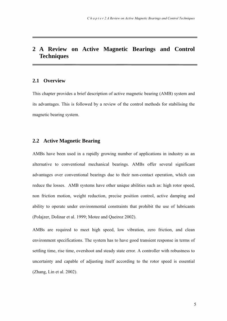
The device for this research is the MBC 500 magnetic bearing system. The MBC 500
consists of two active radial magnetic bearings and a supported rotor mounted on top of
an anodized aluminium case (Magnetic Moments 1995). See Figure 3.1 below.
Figure 3.1 MBC 500 magnetic bearing research experiment Source: (Magnetic Moments 1995)

C h a p t e r 3 Modeling and System Identification of the MBC 500 Magnetic Bearing System
20
The shaft is actively positioned in the radial directions at the shaft ends. It has 4 degrees
of freedom and it is passively centered in the axial direction. Moreover, it freely rotates
about its axis. The magnetic bearing system includes four linear current amplifier pairs
and one pair for each radial bearing axis. In addition, it also includes four internal lead-
lag compensators which independently control the radial bearing axis (Magnetic
Moments 1995).
In addition, the front panel of the MBC 500 magnetic bearing system (shown in Figure
3.2) is a graphical representation of the system dynamics of the MBC 500. The panel
contains 12 BNC connections for easy access to the systems with four inputs and eight
outputs. Moreover, there are four switches in the feedback loops. These switches allow
the user to open the loop for the internal controllers independently. If only one loop is
switched off, the user can perform single-input single-output (SISO) control design
experiments (Magnetic Moments 1995).
Figure 3.2 Front panel block diagram of MBC 500 Source: (Magnetic Moments 1995)

C h a p t e r 3 Modeling and System Identification of the MBC 500 Magnetic Bearing System
21
All the information in this section about the MBC 500 system parameters has been
directly taken from the MBC 500 Magnetic Bearing System Operating Instruction
Manual (Magnetic Moments 1995). This section describes the blocks given on the front
panel of the MBC 500 magnetic bearing system in greater detail. These models given
below are nominal and serve as a guide only. The shaft’s schematic showing
electromagnets and Hall-effect sensors, is provided in Figure 3.3 below.
Figure 3.3 Shaft schematic showing electromagnets and Hall-effect sensors Source: (Magnetic Moments 1995)
• Shaft parameters
The shaft on the MBC 500 is made from non-magnetic 303 stainless steel with a
modulus of elasticity 28 x 106 psi, density 0.29 lb/in3, diameter 0.490 inches
(1.2446cm), and length 10.6 inches (26.924 cm). The bearings are centred 0.95 inches
(2.413 cm) from the shaft ends, and the Hall sensors are centred 0.11 inches (0.2794
cm) from the shaft ends (Magnetic Moments 1995).
C h a p t e r 3 Modeling and System Identification of the MBC 500 Magnetic Bearing System
22
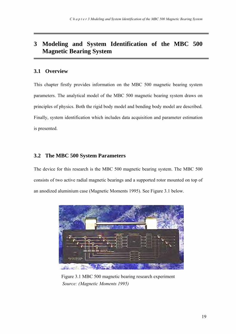
• Bearing parameters
The bearing coils have a 0.5 Amp bias upon which a control signal is superimposed.
The force applied by a single horseshoe electromagnet can be determined by the
formula:
F = k(icontrol + 0.5)2/g2 (Magnetic Moments 1995)......................................................... 3.1
Where k = 2.8 x 10⁻⁷ Nm2/A2, icontrol
is the control current supplied by the current
amplifier in addition to the 0.5A bias current, and g is the air gap in meters. The bias
current in opposing electromagnets has an opposite sign and when the control current is
added to both coils, the net force generated by opposing electromagnets can be
calculated as (Magnetic Moments 1995):
21
2
21
2
)0004.0()5.0(
)0004.0()5.0(
−
−
−
+ −=xi
xi
xcontrolcontrol kkF
...................................................... 3.2 Where x1 is the displacement of the shaft inside the left bearing of Figure 3.3. The same
expression holds for bearing 2 and the y forces as well.
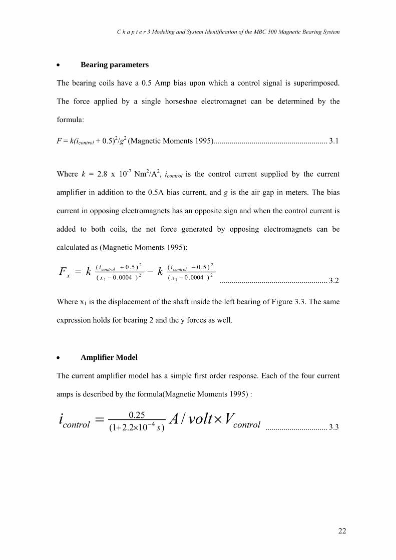
• Amplifier Model
The current amplifier model has a simple first order response. Each of the four current
amps is described by the formula(Magnetic Moments 1995) :
controlscontrol VvoltAi ×= −×+/
)102.21(25.0
4 ............................... 3.3

C h a p t e r 3 Modeling and System Identification of the MBC 500 Magnetic Bearing System
23
• Compensator Model
The nominal compensator model is derived from the circuit schematic and relates
controlV to senseV by the following transfer function (Magnetic Moments 1995):
sensesss
control VV)102.21)(103.31(
)109.81(41.154
4
−−
−
×+×+
×+=............................. 3.4
This compensator can be implemented in an external controller, but time needs to be
considered in tuning the controller due to the nonlinear unstable system.
• Sensor Nonlinearity
The displacements sensed by the two opposing Hall-effect sensors shown in Figure 3.3
are combined electronically to yield the following relationship between shaft end
displacements X1, X2, Y1, or Y2. Expressed in terms of X1, we approximately have:
Vsense = 5 Volts/mmX1 + 24 Volts/mm3 X13 ± 1 Volt offset.
Vsense is available on the front panel via the sensor output BNC connector.
Since the magnetic bearing system is inherently unstable, it is necessary to use
automatic control to keep the system stabilised. To stabilise the system, the position of
the rotor needs to be sensed and the controller must control the amount of current onto
the magnets.

C h a p t e r 3 Modeling and System Identification of the MBC 500 Magnetic Bearing System
24
3.3 Analytical Model of the Magnetic Bearing System
Morse, Smith & Paden (1996) provide the details for the derivation of the analytical
model of the MBC 500 magnetic system. This section provides a brief review of the
analytical model found based on the physical laws of active magnetic bearing.
Analytical Model Derivation
An analytical model is needed in model based control system design. The physics
governing the AMB can be described by differential equations, which represent the
motion of the AMB in response to certain input signals. This will be in the form of a
state space model. A “state-space” model of the system keeps the form of:
BuAx +=χ .................................................................................................................. 3.5 DuCxy += .................................................................................................................. 3.6
Where x is the state vector, u is the system input vector and y is the system output. The
A, B, C and D matrices describe the system mathematically.
For the MBC 500 system, the analytical derivation is broken into two parts: ‘Rigid
Body’ and “Bending Body’. When the system acts as a ‘Rigid Body’ it means that it
remains completely inflexible. When the system acts as a ‘Bending Body’ it means that
it is flexible in rotor motion. Then, MATLAB will be used to compile the models and
determine the characteristics (Morse, Smith et al. 1995). A diagram of the MBC 500
system configuration is shown in Figure 3.4.

C h a p t e r 3 Modeling and System Identification of the MBC 500 Magnetic Bearing System
25
Figure 3.4 MBC 500 system configuration Source: (Morse, Smith et al. 1995)
This MBC 500 system contains a stainless steel shaft or rotor. The rotor or a stainless
steel shaft can levitate using eight “horseshoe” electromagnets with four at each of the
rotor. Hall effect sensors placed just outside of the electromagnets at each end of the
rotor measure the rotor end displacement. The rotor movement is controlled in four
degrees of freedom. This four degrees of freedom are broken into two translational
degrees, including translation in the horizontal direction, 1x and 2x , perpendicular to the
z axis, and translation in the vertical direction, 1y and 2y . Also included in the MBC
500 are four on-board controllers which levitate the bearing when the controllers are
connected in feedback. There are also four switches on the front panel of the MBC 500
to disconnect each of the controllers so that any one or all of them can be replaced by an
external controller (Morse, Smith et al. 1995).
Rigid Body Model
The first analysis of the system assumes that the rotor acts as a rigid body. The
definition of a rigid body is that the rotor does not change shape, which implies that the
rotor does not bend but experiences only transitional or rotational motion. Moreover,
the horizontal and vertical dynamics, i.e. the x and y directions, are uncoupled. The

C h a p t e r 3 Modeling and System Identification of the MBC 500 Magnetic Bearing System
26
effects of coupling cannot be ignored if the rotor were spinning or if the actuators or
sensors were misaligned. Theoretically, the system operates identically in the x and y
directions if their dynamics are uncoupled. However, the additional constant force of
gravity acts in the y direction. The force is non-linear, consequently it cannot be
modeled by a linear system model. For this reason, the analysis of the gravity effect in
the linear y direction is neglected. As mentioned earlier, that the x and y directions are
identical, the derivation is focused on the horizontal or x direction motion. The system
configuration is shown in Figure 3.5, while the parameters are defined in Table 3.1 and
the system variables are described in Table 3.2 (Morse, Smith et al. 1995).
Figure 3.5 Rotor configuration Source: (Magnetic Moments 1995)
Symbol Description
x0 The horizontal displacements of the centre of mass of the rotor
x1 and x2 The horizontal displacements of the rotor at left and right bearing positions, respectively
X1 and X2 The horizontal displacements of the rotor at left and right Hall-effect sensor positions, respectively
ө The angle that the long axis of the rotor makes with the z axis
F1 and F2 The forces exerted on the rotor by left and right bearings, respectively
Table 3.1 System variables Source: (Magnetic Moments 1995)

C h a p t e r 3 Modeling and System Identification of the MBC 500 Magnetic Bearing System
27
Symbol Description Value
L Total length of the rotor 0.269 m l Distance from each bearing to the end of the rotor 0.024 m
l2 Distance from Hall-effect sensor to the end of the rotor 0.0028 m
I0
Moment of inertia of the rotor with respect to rotation about an axis in the y direction
1.5884 × 10⁻³ kgm2
M Mass of the rotor 0.269 kg Table 3.2 System parameters Source: (Magnetic Moments 1995)
To translate the rotor nominal position, that is, the desired rotor position corresponds to
01 =x and 02 =x or equivalently 01 =X and 02 =X or 00 =x and 0=θ . The rotor
will be centered horizontally with respect to the front and back electromagnets on each
end, and its long axis is parallel to the z axis. In addition, the rotor end displacements
are expressed as shown below (Morse, Smith et al. 1995):
θsin)( 201 lxx L −−= ..................................................................................................... 3.7 θsin)( 202 lxx L −+= .................................................................................................... 3.8 θsin)( 2201 lxX L −−= .................................................................................................. 3.9 θsin)( 2202 lxX L −+= ............................................................................................... 3.10
Assume that θ is small, this is a valid assumption considering the physical dimension
of the system. The first order approximations are: sin θθ ≅ and cos 1≅θ .
Newton’s law is used to find the equations of motion for rigid body mechanical
systems. In addition, the force balance equation is used for the rotor analysis as shown
20 12
1 mLI =

C h a p t e r 3 Modeling and System Identification of the MBC 500 Magnetic Bearing System
28
below (Morse, Smith et al. 1995):
→→
=∑ amF .................................................................................................................. 3.11
where ∑→
F is the summation of all external forces applied to the system, m is the rotor
mass, and →
a is the acceleration of the centre of gravity of the system.
The moment balance can be expressed as:
→→
=∑ αIM .................................................................................................................. 3.12
where ∑→
M is the summation of all moments applied externally to the system, I is the
rotational moment of inertia of the system about the axis through the centre of gravity
and in the direction of rotation, and →
α is the angular acceleration of the system.
The moments and forces are interrelated as shown in the following equation:
→→→
= FxrM ................................................................................................................... 3.13
where →
r is any vector pointing from point 0 to the line of application of the force →
F .
This relationship is shown pictorially in Figure 3.6a below.
However, if the vector →
r is chosen to be perpendicular to the line of application of the
force →
F as shown in Figure 3.6b, then the above equation reduces to
M=rF ........................................................................................................................... 3.14

C h a p t e r 3 Modeling and System Identification of the MBC 500 Magnetic Bearing System
29
As can be seen in Figure 3.6, the sense of the moment is counter-clockwise. From the
force and moment balance equations above, the non-linear differential equations can be
derived governing the rigid body motion as shown in Figure 3.5 above. The motion is
only in one plane which is the x direction. The equations of motion are shown below:
210 FFxmF +==⋅⋅
∑ ................................................................................................. 3.15
θθθ cos)(cos)( 21220 lFlFIM LL −−−==⋅⋅
∑ ........................................................... 3.16
Figure 3.6a Figure 3.6b
Figure 3.6 Force/Moment relationships Source: (Morse, Smith et al. 1995)
All the above differential equations, system parameters and variables have been used in
order to determine a suitable model for the rigid body system. This useful information
was obtained through doing a series of exercises set in the MBC500 manual. The final
result took the form of a two-input, two-output state space representation in the form:

C h a p t e r 3 Modeling and System Identification of the MBC 500 Magnetic Bearing System
30
⎥⎥⎥⎥⎥⎥⎥⎥⎥
⎦
⎤
⎢⎢⎢⎢⎢⎢⎢⎢⎢
⎣
⎡
⋅
⋅
⋅⋅
⋅
2
1
0
..0
.
control
control
i
i
xx
θθ = rA
⎥⎥⎥⎥⎥⎥⎥⎥
⎦
⎤
⎢⎢⎢⎢⎢⎢⎢⎢
⎣
⎡
⋅
2
1
0
.0
control
control
ii
x
x
θθ
+ rB ⎥⎦
⎤⎢⎣
⎡
2
1
control
control
VV
.................................................................... 3.17
⎥⎥⎥⎥⎥⎥⎥⎥
⎦
⎤
⎢⎢⎢⎢⎢⎢⎢⎢
⎣
⎡
=⎥⎦
⎤⎢⎣
⎡⋅
2
1
0
.0
2
1
control
control
rsense
sense
ii
x
x
CVV
θθ
........................................................................................ 3.18
where rA , rB and rC are the state space matrices for the rigid body case. From this
result, the system response has been determined.
The manual of MBC 500 provides the following nominal transfer function for each of
the on-board controllers:
iii sensesensecontrol VsCVss
sV )()102.21)(103.31(
)109.81(41.154
4
=×+×+
×+= −−
−
............................... 3.19
For the controller design, the controller )(1 sCx is replaced by mapping 1senseV to 1controlV .
The system seen by the controller is as shown in Figure3.7. However, because of the
rigid body is a simplified version in that the x and y rotor motion are uncoupled, an
equivalent system configuration is shown in Figure 3.8.

C h a p t e r 3 Modeling and System Identification of the MBC 500 Magnetic Bearing System
31
Figure 3.7 Bearing system seen by controller xCx −1 and y directions coupled
Source: (Morse, Smith et al. 1995)
Figure 3.8 Bearing system seen by controller xCx −1 and y directions uncoupled Source: (Morse, Smith et al. 1995)
In order to obtain the analytical model for the rigid body system to be controlled, the
controllers )(2 sCx , )(1 sCy and )(2 sCy must be included in the feedback as shown in
Figure 3.7. Specific commands in MATLAB can convert the controller model C(s) to a
state space model. This state space model has controller matrices acont, bcont, ccont
and dcont representing the on-board controllers.
From the equation 3.15, it can be obtained that:
mF
mF 21
0 +=⋅⋅
χ .............................................................................................................. 3.20

C h a p t e r 3 Modeling and System Identification of the MBC 500 Magnetic Bearing System
32
Since θ is small so 1cos ≈θ and θ becomes:
20
100
21
0
22 )2
(1)2
(1)()(FlL
IFlL
IIlF
IlF LL
−+−−=−
−−
=⋅⋅
θ ........................................... 3.21
Meanwhile, assuming θ is small so X1 and X2 can be simplified as follows by using the
equations 3.5 and 3.6:
θ)( 2201 lxX L −−= ..................................................................................................... 3.22 θ)( 2202 lxX L −+= ..................................................................................................... 3.23
All the equations above can be written in state space form with the state vector:
⎥⎥⎥⎥⎥
⎦
⎤
⎢⎢⎢⎢⎢
⎣
⎡
==⋅
θθ
0
.0
x
x
xx r
where r means rigid body. In addition, F1 and F2 represent input variables and X1 and X2
are output variables, the state space equations can be written as follows:
⎥⎦
⎤⎢⎣
⎡
⎥⎥⎥⎥⎥
⎦
⎤
⎢⎢⎢⎢⎢
⎣
⎡
−
+
⎥⎥⎥⎥⎥
⎦
⎤
⎢⎢⎢⎢⎢
⎣
⎡
⎥⎥⎥⎥
⎦
⎤
⎢⎢⎢⎢
⎣
⎡
=
⎥⎥⎥⎥⎥
⎦
⎤
⎢⎢⎢⎢⎢
⎣
⎡
−−
⋅⋅⋅
⋅2
1
)(1
)(1
110
.0
0
..0
.
2020
00
00
0000100000000010
FFx
x
xx
lIlI
mm
LLθθ
θθ ................................................... 3.24
⎥⎥⎥⎥⎥
⎦
⎤
⎢⎢⎢⎢⎢
⎣
⎡
⎥⎦
⎤⎢⎣
⎡−−−
=⎥⎦
⎤⎢⎣
⎡
⋅
θθ
0
.0
22
22
2
1
0)(010)(01 x
x
ll
XX
l
l
............................................................................. 3.25

C h a p t e r 3 Modeling and System Identification of the MBC 500 Magnetic Bearing System
33
Clearly, it can be seen that all four eigenvalues are 0 for the state matrix.
By implementing the first order approximation at the point (0,0) to describe the bearing
force on the rotor:
)0()0,0()0()0,0()0,0(),( −⎥⎦
⎤⎢⎣
⎡∂∂
+−⎥⎦
⎤⎢⎣
⎡∂∂
+= controlicontroli
ii
i
iicontroliii i
iF
xxF
FixF .................. 3.26
The ith non-linear be
Bearing force can be expressed as (Magnetic Moments 1995):
2
2
2
2
)0004.0()5.0(
)0004.0()5.0(
+
−−
−
+=
i
control
i
controli x
ik
xi
kF ii .................................................................... 3.27
where k=2.8 x 10⁻⁷ Nm2/Amp2.
i
i
xF∂∂ can be found as follows:
⎟⎟⎠
⎞⎜⎜⎝
⎛+
−−−
−+−
=∂∂
3
2
3
2
)0004.0()5.0(2
)0004.0()5.0(2
i
controli
i
controli
i
i
xi
xi
kxF
....................................................... 3.28
and
4375)0,0(
=∂∂
i
i
xF
........................................................................................................... 3.29
controli
i
iF
∂∂ can be derived as:
⎟⎟⎠
⎞⎜⎜⎝
⎛+
−−
−+
=∂∂
22 )0004.0()5.0(2
)0004.0()5.0(2
i
controli
i
controli
controli
i
xi
xi
ki
F........................................................... 3.30
and
5.3)0,0(
=∂∂
controli
i
iF
......................................................................................................... 3.31

C h a p t e r 3 Modeling and System Identification of the MBC 500 Magnetic Bearing System
34
F1 and F2 can thus be expressed as:
111 5.34375 controlixF += ..................................................................................... 3.32
222 5.34375 controlixF += ........................................................................................ 3.33
Combining equation 3.7 with equation 3.32, F1 and F2 can be expressed as follows:
1201 5.3)(43754375 controlL ilxF +−−= θ ........................................................... 3.34
Combining equation 3.8 with equation 3.33, F1 and F2 can be expressed as follows:
2202 5.3)(43754375 controlL ilxF +−+= θ ............................................................. 3.35
0
..x can be written as:
milx
milx
x controlL
controlL
2201200
.. 5.3)(437543755.3)(43754375 +−++
+−−=
θθ
mi
mi
xm
x controlcontrol 2100
.. 5.35.38750++= ............................................................... 3.36
Meanwhile, ⋅⋅
θ can be expressed as:
( ) ( )2200
1200
5.3)(43754375)2
(15.3)(43754375)2
(1control
Lcontrol
L ilxlLI
ilxlLI
+−+−++−−−−=⋅⋅
θθθ
20
21
0
2
0
22 )(
5.3)(
5.3)(
8750 control
L
control
LL
iI
li
Il
Il θθθ
θ−
+−
−−
=⋅⋅
........................................ 3.37

C h a p t e r 3 Modeling and System Identification of the MBC 500 Magnetic Bearing System
35
Therefore, the new state space rigid body system model including the actuator dynamics
with 1controli and 2controli as input variables can be expressed below:
⎥⎦
⎤⎢⎣
⎡
⎥⎥⎥⎥⎥
⎦
⎤
⎢⎢⎢⎢⎢
⎣
⎡
−−−
+
⎥⎥⎥⎥⎥
⎦
⎤
⎢⎢⎢⎢⎢
⎣
⎡
⎥⎥⎥⎥⎥
⎦
⎤
⎢⎢⎢⎢⎢
⎣
⎡
=
⎥⎥⎥⎥⎥
⎦
⎤
⎢⎢⎢⎢⎢
⎣
⎡
−⋅⋅
⋅2
1
25.3
25.3
5.35.30
.0
)(8750
87500
..0
.
)()(00
00
00010000000010
000
22
control
control
LI
LI
mm
Il
m
ii
ll
x
x
xx
L
θθ
θθ
&
................ 3.38
⎥⎥⎥⎥⎥
⎦
⎤
⎢⎢⎢⎢⎢
⎣
⎡
⎥⎦
⎤⎢⎣
⎡−−−
=⎥⎦
⎤⎢⎣
⎡
⋅
θθ
0
.0
22
22
2
1
0)(010)(01 x
x
ll
XX
L
L
.................................................................... 3.39
Using the system parameters given in Table 3.2, the eigenvalues of the state matrix are:
sec4.1822629.0
87508750 rad
m±=±=± ;
sec3
2
0
22 4.259
10*5884.11105.08750)(8750 rad
L
Il
±=×
±=−×
± −
As can be seen, the system is unstable because there are two positive eigenvalues.
Another implementation of Taylor series approximation at the 0=ix can be used to
linearise the sensor non-linearity:
)0()0()0()( −⎥⎦
⎤⎢⎣
⎡∂
∂+= i
i
senseisenseiisensei X
XV
VXV ...................................................... 3.40
Where the relationship between the voltage sensed and the rotor displacement is given
below (Magnetic Moments, 1995):
39 )1025(5000 iisense XXVi
×+= .................................................................................. 3.41

C h a p t e r 3 Modeling and System Identification of the MBC 500 Magnetic Bearing System
36
i
sensei
XV∂
∂ can be calculated as:
29 )1025(35000 ii
sensei XX
V×+=
∂∂
................................................................................. 3.42
5000)0(
=∂
∂
i
sensei
XV
........................................................................................................ 3.43
As the result: isensei XV 5000= ..................................................................................... 3.44
The output equation becomes:
rL
L
sense
sense xll
VV
⎥⎦
⎤⎢⎣
⎡−−−
=⎥⎦
⎤⎢⎣
⎡0)(010)(01
500022
22
2
1............................................................... 3.45
Since the sensor transfer function is purely a gain, the eigenvalues of the system are not
affected. Furthermore, the magnetic bearing manual gives the dynamic characteristics of
current amplifiers:
controlicontrolicontroli Viidtd
44 102.225.0
102.21)( −− ×
+×
−=
The amplifier input is controliV and its output is controlii . 1controlV and 2controlV are the voltages
that the controller produces to control the bearing. The current amplifier is a low pass
filter, the range of frequencies passed by the current amplifier is from 0 to 4545 secrad .
By adding the current amplifier dynamics to the rigid body model obtained above, let
1controlV and 2controlV as input variables and 1senseV and 2senseV as output variables.
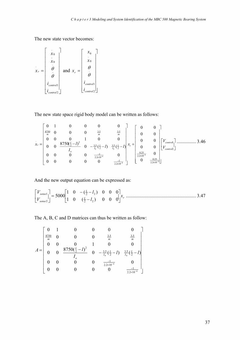
C h a p t e r 3 Modeling and System Identification of the MBC 500 Magnetic Bearing System
37
The new state vector becomes:
⎥⎥⎥⎥⎥⎥⎥⎥
⎦
⎤
⎢⎢⎢⎢⎢⎢⎢⎢
⎣
⎡
= ⋅⋅
⋅⋅
2
1
0
..0
.
control
control
r
ii
xx
xθθ and
⎥⎥⎥⎥⎥⎥⎥⎥
⎦
⎤
⎢⎢⎢⎢⎢⎢⎢⎢
⎣
⎡
= ⋅
2
1
0
.0
control
control
r
ii
x
x
xθθ
The new state space rigid body model can be written as follows:
⎥⎦
⎤⎢⎣
⎡
⎥⎥⎥⎥⎥⎥⎥⎥
⎦
⎤
⎢⎢⎢⎢⎢⎢⎢⎢
⎣
⎡
+
⎥⎥⎥⎥⎥⎥⎥⎥
⎦
⎤
⎢⎢⎢⎢⎢⎢⎢⎢
⎣
⎡
−−−−=
−
−
−
−
×
×
×−
×−
2
1
102.225.0
102.225.0
102.21
102.21
25.3
25.3
22
5.35.38750
.
4
4
4
4
00
0000000000
0000000000
)()(0)(875000
001000000
000010
control
controlrL
IL
Io
L
mmm
rVV
xllI
lx ................ 3.46
And the new output equation can be expressed as:
rL
L
sense
sense xll
VV
⎥⎦
⎤⎢⎣
⎡−−−
=⎥⎦
⎤⎢⎣
⎡000)(01000)(01
500022
22
2
1 .......................................................... 3.47
The A, B, C and D matrices can thus be written as follow:
⎥⎥⎥⎥⎥⎥⎥⎥
⎦
⎤
⎢⎢⎢⎢⎢⎢⎢⎢
⎣
⎡
−−−−=
−
−
×−
×−
4
4
00
102.21
102.21
25.3
25.3
22
5.35.38750
0000000000
)()(0)(875000
001000000
000010
llI
lA LI
LI
o
L
mmm

C h a p t e r 3 Modeling and System Identification of the MBC 500 Magnetic Bearing System
38
⎥⎥⎥⎥⎥⎥⎥⎥
⎦
⎤
⎢⎢⎢⎢⎢⎢⎢⎢
⎣
⎡
=
−
−
×
×
4
4
102.225.0
102.225.0
0000000000
B , ⎥⎦
⎤⎢⎣
⎡−−−
=000)(01000)(01
500022
22
ll
CL
L
and ⎥⎦
⎤⎢⎣
⎡=
0000
D
The eigenvalues of the A matrix of the model obtained above correspond to the rigid
body rotor modes and the current amplifier dynamics. These eigenvalues are the poles
of the system. Table 3.3 gives the eigenvalues and their corresponding pole location on
the s-plane.
Mode/Dynamic Eigenvalues
Rigid body rotor 182.4
Rigid body rotor -182.4
Rigid body rotor 259.4
Rigid body rotor -259.4
Current amplifier -4545.5
Current amplifier -4545.5
Table 3.3 Pole locations of the Rigid Body model
From the magnetic bearing manual, the nominal transfer function for each of the on-
board controllers is:
.)()102.21)(103.31(
)109.81(41.154
4
senseisenseicontroli VsCVss
sV =×+×+
×+= −−
−
Finally, the specific commands in MATLAB convert the controller model C(s) to a state
space model. This state space model has controller matrices acont, bcont, ccont and
dcont representing the on-board controllers.
The MATLAB commands below are the rigid body analytical model for the system and
it will be referred to as the “rigid body model” hereafter.
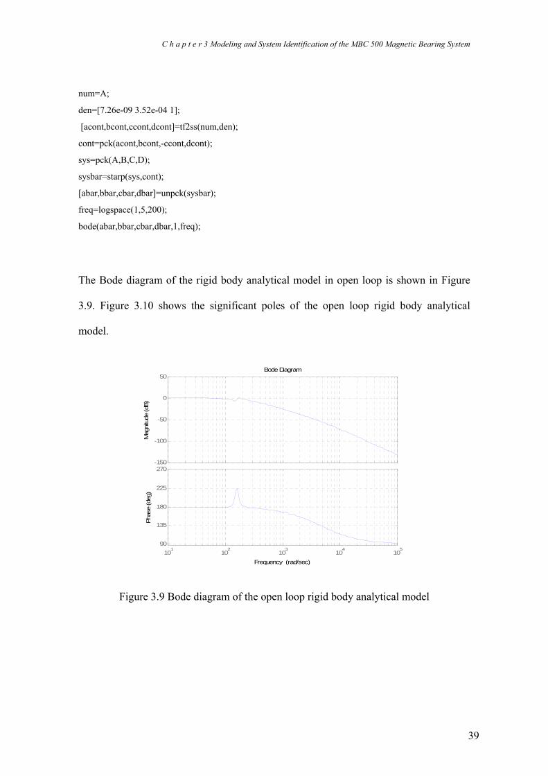
C h a p t e r 3 Modeling and System Identification of the MBC 500 Magnetic Bearing System
39
num=A;
den=[7.26e-09 3.52e-04 1];
[acont,bcont,ccont,dcont]=tf2ss(num,den); cont=pck(acont,bcont,-ccont,dcont); sys=pck(A,B,C,D); sysbar=starp(sys,cont); [abar,bbar,cbar,dbar]=unpck(sysbar); freq=logspace(1,5,200); bode(abar,bbar,cbar,dbar,1,freq);
The Bode diagram of the rigid body analytical model in open loop is shown in Figure
3.9. Figure 3.10 shows the significant poles of the open loop rigid body analytical
model.
-150
-100
-50
0
50
Mag
nitu
de (d
B)
101
102
103
104
105
90
135
180
225
270
Phas
e (d
eg)
Bode Diagram
Frequency (rad/sec)
Figure 3.9 Bode diagram of the open loop rigid body analytical model

C h a p t e r 3 Modeling and System Identification of the MBC 500 Magnetic Bearing System
40
-5000 -4000 -3000 -2000 -1000 0 1000-1
-0.8
-0.6
-0.4
-0.2
0
0.2
0.4
0.6
0.8
1Pole-Zero Map
Real Axis
Imag
inar
y Ax
is
Figure 3.10 Significant poles of the open loop rigid body analytical model
Bending Body Model
In the previous analysis, it was assumed that the rotor is a rigid body. However, during
levitation, the rotor does experience some bending. In this section, only two modes of
the lowest frequency of bending mode will be modeled. These bending modes are
described in Figure 3.11.
Figure 3.11 Two bending modes taken into account Source: (Morse, Smith et al. 1995)

C h a p t e r 3 Modeling and System Identification of the MBC 500 Magnetic Bearing System
41
The bending model assumes that no rigid body motion is excited in the system; hence
an equation of motion can be obtained by describing the system motion strictly due to
the rotor bending. To achieve this equation, some matrices must be defined (Morse,
Smith et al. 1995).
A vector of amplitude variables is defined by:
⎥⎦
⎤⎢⎣
⎡≡
2
1
aa
a ...................................................................................................................... 3.48
Rotor displacements are defined by:
⎢⎣
⎡+−+−
=⎥⎦
⎤⎢⎣
⎡0093745.10093745.1
2
1
ee
XX
⎥⎦
⎤++−0083546.10083546.1
ee
a............................................................ 3.49
⎢⎣
⎡+−+−
=⎥⎦
⎤⎢⎣
⎡0019029.10019029.1
2
1
ee
xx
⎥⎦
⎤−−−−
0108354.60108354.6
ee
a ............................................................ 3.50
Mass matrix is defined by:
⎢⎣
⎡ −=
00172146.2 e
M ⎥⎦
⎤− 0162297.2
0e
....................................................................... 3.51
Stiffness matrix is defined by:
⎢⎣
⎡ +=
00605762.6 e
K ⎥⎦
⎤+ 074363.4
0e
........................................................................... 3.52
A vector forcing function is defined by:
⎢⎣
⎡−−+−
=0108354.60019029.1
ee
P ⎥⎦
⎤⎢⎣
⎡⎥⎦
⎤−+−
2
1
0108354.60019029.1
FF
ee
............................................................. 3.53

C h a p t e r 3 Modeling and System Identification of the MBC 500 Magnetic Bearing System
42
The following differential equation describes the bending motion of the rotor:
PKaaM =+⋅⋅
.............................................................................................................. 3.54 There are similarities between the differential equation given above and the standard
differential equation of motion for a spring/mass system. Hence, the rotor behaves much
like an interconnection of springs and masses in bending mode (Morse, Smith et al.
1995).
From the differential equations described above, a state vector for the flexible body is
defined as;
⎥⎥⎥⎥⎥⎥
⎦
⎤
⎢⎢⎢⎢⎢⎢
⎣
⎡
=
⋅⋅
⋅⋅
⋅
⋅
2
1
2
1
.
a
a
a
a
x f
As in the case of the rigid body, F1 and F2 are the input variables and X1 and X2 are the
output variables. The bending mode equations expressed in state space form are as
below:
⎥⎦
⎤⎢⎣
⎡
⎥⎥⎥⎥
⎦
⎤
⎢⎢⎢⎢
⎣
⎡
+
⎥⎥⎥⎥
⎦
⎤
⎢⎢⎢⎢
⎣
⎡
=
−
−−
−
−
⋅
2
1
262297.0608354.0
262297.0608354.0
272146.019029.1
272146.019029.1
262297.074363.4
272146.0605762.6
0000
00000010000100
FF
xx f
e
ef ............................... 3.55
fxXX
⎥⎦
⎤⎢⎣
⎡−
−−=⎥
⎦
⎤⎢⎣
⎡0083546.193745.10083546.193745.1
2
1........................................................... 3.56
The frequencies of oscillation are: sec
7
13005262297.0
104363.4 radj±=×−
± and
.4718272146.0
1005762.6sec
6radj±=
×−±
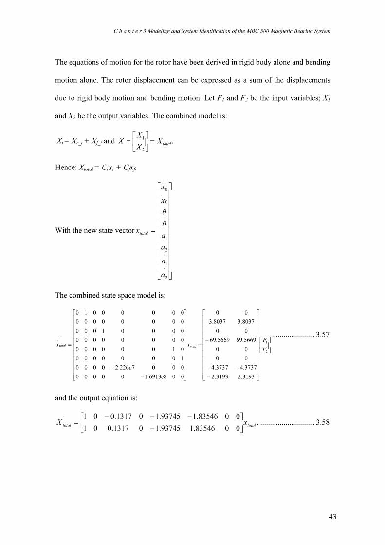
C h a p t e r 3 Modeling and System Identification of the MBC 500 Magnetic Bearing System
43
The equations of motion for the rotor have been derived in rigid body alone and bending
motion alone. The rotor displacement can be expressed as a sum of the displacements
due to rigid body motion and bending motion. Let F1 and F2 be the input variables; X1
and X2 be the output variables. The combined model is:
Xi = Xr_i + Xf_i and .2
1totalX
XX
X =⎥⎦
⎤⎢⎣
⎡=
Hence: Xtotal = Crxr + Cfxf.
With the new state vector
⎥⎥⎥⎥⎥⎥⎥⎥⎥⎥⎥⎥
⎦
⎤
⎢⎢⎢⎢⎢⎢⎢⎢⎢⎢⎢⎢
⎣
⎡
=
⋅
⋅
⋅
2
1
2
1
0
.0
a
a
aa
x
x
xtotal
θθ
The combined state space model is:
⎥⎦
⎤⎢⎣
⎡
⎥⎥⎥⎥⎥⎥⎥⎥⎥⎥⎥
⎦
⎤
⎢⎢⎢⎢⎢⎢⎢⎢⎢⎢⎢
⎣
⎡
−−−
−+
⎥⎥⎥⎥⎥⎥⎥⎥⎥⎥⎥
⎦
⎤
⎢⎢⎢⎢⎢⎢⎢⎢⎢⎢⎢
⎣
⎡
−−
=⋅
2
1.
3193.23193.23737.43737.400005669.695669.6900
8037.38037.300
0086913.1000000007226.20000100000000100000000000000000010000000000000000010
FF
x
ee
x totaltotal
...................... 3.57
and the output equation is:
.0083546.193745.101317.0010083546.193745.101317.001
totaltotal xX ⎥⎦
⎤⎢⎣
⎡−
−−−=
⋅
............................ 3.58

C h a p t e r 3 Modeling and System Identification of the MBC 500 Magnetic Bearing System
44
Using the linear approximations to the input and output non-linearities obtained
previously and adding the actuator and sensor dynamics to the combined model
described in equations 3.52 and 3.53, the new state space equation can be written as
follows with 1controli and 2controli as input variables, and 1sensev and 2sensev as output
variables:
⎥⎦
⎤⎢⎣
⎡
⎥⎥⎥⎥⎥⎥⎥⎥⎥⎥⎥
⎦
⎤
⎢⎢⎢⎢⎢⎢⎢⎢⎢⎢⎢
⎣
⎡
−−−+=
××−
×−×−
⋅
2
1
262297.0608354.05.3
262297.0608354.05.3
272146.019029.15.3
272146.019029.15.3
25.3
25.3
5.35.3
0000
)()(00
00
00
control
controlL
IL
I
mm
totaltotaltotaliill
xAx with ........................................... 3.59
⎥⎥⎥⎥⎥⎥⎥⎥⎥⎥⎥
⎦
⎤
⎢⎢⎢⎢⎢⎢⎢⎢⎢⎢⎢
⎣
⎡
××−×−=
+−×−
×+−×−
×−
000000
000000100000000100000000608354.08750)(008750)(000000100000000000000010
262297.0608354.0*875074363.4
262297.0
608354.08750*)(272146.0
19029.18750605762.6272146.0
19029.18750
212
21
19029.187508750
22
2
00
el
e
LI
LI
mm
total
L
llA
................... 3.60
The sensor dynamic only changes the output equation with the gain of 5000:
totalL
L
sense
sense xll
VV
⎥⎦
⎤⎢⎣
⎡−−
−−−−=⎥
⎦
⎤⎢⎣
⎡0083546.193745.10)(010083546.193745.10)(01
500022
22
2
1

C h a p t e r 3 Modeling and System Identification of the MBC 500 Magnetic Bearing System
45
Adding the current amplifier dynamics described previously and letting 1controlV and
2controlV be input variables; and 1senseV and 2senseV output variables, with the new state
vector can be expressed as:
⎥⎥⎥⎥⎥⎥⎥⎥⎥⎥⎥⎥⎥⎥⎥
⎦
⎤
⎢⎢⎢⎢⎢⎢⎢⎢⎢⎢⎢⎢⎢⎢⎢
⎣
⎡
=
⋅
⋅
⋅
2
1
2
1
2
1
0
.0
control
control
total
ii
a
a
aa
x
x
x
θθ
and the new dynamic matrix
⎥⎥⎥⎥⎥⎥⎥⎥⎥⎥⎥⎥⎥⎥
⎦
⎤
⎢⎢⎢⎢⎢⎢⎢⎢⎢⎢⎢⎢⎢⎢
⎣
⎡
−−−××−×−
=
−−
−−
××−×+−××−
×−×−×+−×−
×−
42.21
42.21
262297.0608354.05.3
262297.0608354.05.3
262297.0608354.0875074363.4
262297.0608354.08750)(
272146.019029.15.3
272146.019029.15.3
272146.019029.18750605762.6
272146.019029.18750
25.3
25.3
212
21
5.35.319029.187508750
000000000000000000
000000000000
00100000000001000000
)()(00608354.08750)(008750)(000000001000
0000000000000010
22
2
0000
e
e
el
e
LI
LI
LI
LI
mmmm
total
L
llll
A
. 3.61
The total body model state space description becomes:
⎥⎦
⎤⎢⎣
⎡
⎥⎥⎥⎥⎥⎥⎥⎥⎥⎥⎥⎥⎥⎥
⎦
⎤
⎢⎢⎢⎢⎢⎢⎢⎢⎢⎢⎢⎢⎢⎢
⎣
⎡
+=
−
−
2
1
42.225.0
42.225.0
.
000000000000000000
control
control
e
e
totaltotaltotalVV
xAx ................................................................... 3.62
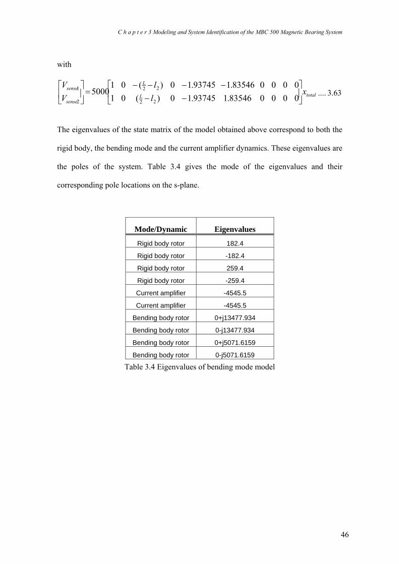
C h a p t e r 3 Modeling and System Identification of the MBC 500 Magnetic Bearing System
46
with
totalL
L
sense
sense xll
VV
⎥⎦
⎤⎢⎣
⎡−−
−−−−=⎥
⎦
⎤⎢⎣
⎡000083546.193745.10)(01000083546.193745.10)(01
500022
22
2
1.... 3.63
The eigenvalues of the state matrix of the model obtained above correspond to both the
rigid body, the bending mode and the current amplifier dynamics. These eigenvalues are
the poles of the system. Table 3.4 gives the mode of the eigenvalues and their
corresponding pole locations on the s-plane.
Mode/Dynamic Eigenvalues
Rigid body rotor 182.4
Rigid body rotor -182.4
Rigid body rotor 259.4
Rigid body rotor -259.4
Current amplifier -4545.5
Current amplifier -4545.5
Bending body rotor 0+j13477.934
Bending body rotor 0-j13477.934
Bending body rotor 0+j5071.6159
Bending body rotor 0-j5071.6159
Table 3.4 Eigenvalues of bending mode model

C h a p t e r 3 Modeling and System Identification of the MBC 500 Magnetic Bearing System
47
Using the MATLAB commands below, the total system model can be obtained and it
will be referred to as the “total system model” hereafter:
num=[1.25e-03 1.41]; den=[7.26e-09 3.52e-04 1]; [acont,bcont,ccont,dcont]=tf2ss(num,den); cont=pck(acont,bcont,-ccont,dcont); sysb=pck(ab,bb,cb,db); sysbarb=starp(sysb,cont); [abarb,bbarb,cbarb,dbarb]=unpck(sysbarb); freq=lospace(1,5,200); bode(abarb,bbarb,cbarb,dbarb,1,freq);
⎥⎥⎥⎥⎥⎥⎥⎥⎥⎥⎥⎥⎥⎥
⎦
⎤
⎢⎢⎢⎢⎢⎢⎢⎢⎢⎢⎢⎢⎢⎢
⎣
⎡
−−−××−×−
=
−−
−−
××−×+−××−
×−×−×+−×−
×−
42.21
42.21
262297.0608354.05.3
262297.0608354.05.3
262297.0608354.0875074363.4
262297.0608354.08750)(
272146.019029.15.3
272146.019029.15.3
272146.019029.18750605762.6
272146.019029.18750
25.3
25.3
212
21
5.35.319029.187508750
000000000000000000
000000000000
00100000000001000000
)()(00608354.08750)(008750)(000000001000
0000000000000010
22
2
0000
e
e
el
e
LI
LI
LI
LI
mmmm
b
L
llll
a
⎥⎥⎥⎥⎥⎥⎥⎥⎥⎥⎥⎥⎥⎥
⎦
⎤
⎢⎢⎢⎢⎢⎢⎢⎢⎢⎢⎢⎢⎢⎢
⎣
⎡
=
−
−
42.225.0
42.225.0
000000000000000000
e
e
bb ; ;000083546.193745.10)(01000083546.193745.10)(01
22
22⎥⎦
⎤⎢⎣
⎡−−
−−−−=
ll
cL
L
b and
⎥⎦
⎤⎢⎣
⎡=
0000
bd

C h a p t e r 3 Modeling and System Identification of the MBC 500 Magnetic Bearing System
48
All the values of the variables can be found in Table 3.2.
The Bode diagram of the combined rigid body and bending mode analytical model in
open loop is shown in Figure 3.12. Figure 3.13 shows the significant poles and zeros of
the open loop combined rigid body and bending mode analytical model.
-150
-100
-50
0
50
Mag
nitu
de (d
B)
101
102
103
104
105
-90
0
90
180
270
Phas
e (d
eg)
Bode Diagram
Frequency (rad/sec) Figure 3.12 Bode diagram of the open loop combined rigid body and bending mode
analytical model
-5000 -4000 -3000 -2000 -1000 0 1000-1.5
-1
-0.5
0
0.5
1
1.5x 10
4 Pole-Zero Map
Real Axis
Imag
inar
y Ax
is
Figure 3.13 Significant poles and zeros of the open loop combined rigid body and
bending mode analytical model

C h a p t e r 3 Modeling and System Identification of the MBC 500 Magnetic Bearing System
49
3.4 Magnetic Bearing System Identification
Experimental Set-up
Experimental determination of a system model is an important part of the modeling
process in control engineering. This phase of modeling is referred to as system
identification. The chosen approach to obtain the transfer function of the MBC 500
AMB system was to measure the frequency response of the closed-loop system. As
previously mentioned, an AMB is inherently unstable; this is the reason behind
performing a closed-loop experiment. Figure 3.14 is a block diagram of the setup used
to collect the data.
The output from the function generator is sinusoidal signal with a frequency range of 10
Hz to 3.05 KHz and a peak magnitude of 500mV. A 4 KHz Low Pass Filter (LPF) is
used in order to limit the high frequency noise and a ±10V Voltage Limiter is required
to ensure high voltages do not reach the DSP card. The DSP consists of input-output
channels with analog-to-digital converters (ADC) and digital-to-analog converters
(DAC). The ADC transforms the sinusoidal signal input into discrete form, while the
DAC transforms the discrete form into the sinusoidal signal. The output from the card is
stored in a data file, which contains three data columns, namely, frequency, magnitude
and phase.

C h a p t e r 3 Modeling and System Identification of the MBC 500 Magnetic Bearing System
50
Figure 3.14 Block diagram of a system identification setup Setting-Up the Magnetic Bearing for testing
The magnetic bearing system configuration is as shown on the magnetic bearing front
panel block diagram in Figure 3.15. The bearing system contains four-on-board
controllers. The on-board controllers levitate the bearing (Morse, Smith et al. 1996).
Figure 3.15 Magnetic bearing block diagram Source: (Morse, Smith et al. 1996)
The magnetic bearing is an unstable system. If any on-board controllers are
disconnected, then the rotor will hit the touch-down bushings in the bearing housings
which form a physical limit for the rotor. Because of this instability, any data from the
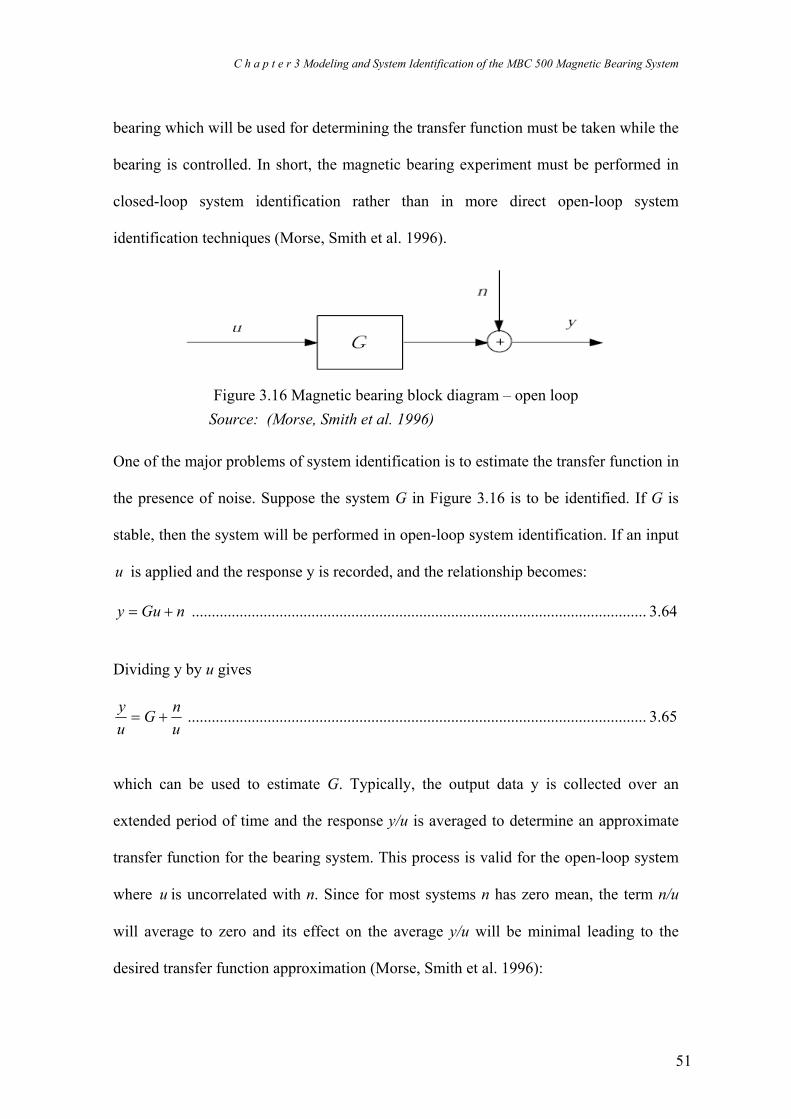
C h a p t e r 3 Modeling and System Identification of the MBC 500 Magnetic Bearing System
51
bearing which will be used for determining the transfer function must be taken while the
bearing is controlled. In short, the magnetic bearing experiment must be performed in
closed-loop system identification rather than in more direct open-loop system
identification techniques (Morse, Smith et al. 1996).
Figure 3.16 Magnetic bearing block diagram – open loop
Source: (Morse, Smith et al. 1996) One of the major problems of system identification is to estimate the transfer function in
the presence of noise. Suppose the system G in Figure 3.16 is to be identified. If G is
stable, then the system will be performed in open-loop system identification. If an input
u is applied and the response y is recorded, and the relationship becomes:
nGuy += .................................................................................................................. 3.64
Dividing y by u gives
unG
uy
+= ................................................................................................................... 3.65
which can be used to estimate G. Typically, the output data y is collected over an
extended period of time and the response y/u is averaged to determine an approximate
transfer function for the bearing system. This process is valid for the open-loop system
where u is uncorrelated with n. Since for most systems n has zero mean, the term n/u
will average to zero and its effect on the average y/u will be minimal leading to the
desired transfer function approximation (Morse, Smith et al. 1996):

C h a p t e r 3 Modeling and System Identification of the MBC 500 Magnetic Bearing System
52
uyG ≅ .......................................................................................................................... 3.66
If, u were correlated with n, then the term n/u would not average to zero and would add
to and corrupt the estimate of G.
For the closed-loop system configuration shown in Figure 3.17, the y/u = G + n/u again
holds; however, the input u can be expressed as follows (Morse, Smith et al. 1996):
nGC
CrGC
u+
−+
=11
1 .............................................................................................. 3.67
Figure 3.17 Magnetic bearing block diagram – closed loop Source: (Dorf and Bishop 1995)
From the above equation, it is clearly showed that u and n are correlated, and therefore
the term n/u will not average to zero as y/u is averaged. Since the effect of the noise on
the system response cannot be neglected, its effect on the system estimate has to be
found. Furthermore, y/u can be expressed in the following way (Morse, Smith et al.
1996):
CnrGrn
uy
−+
= ................................................................................................................. 3.68

C h a p t e r 3 Modeling and System Identification of the MBC 500 Magnetic Bearing System
53
Notice that as n becomes small compared to r, G can be obtained using y/u:
Guy≅ .......................................................................................................................... 3.69
However, if n is large compared to r, then y/u will yield:
Cuy 1
−≅ ...................................................................................................................... 3.70
The actual system data y/u will be somewhere in between G and -1/C. However,
without the exact knowledge of the noise n, G cannot be found. Consequently, the
accuracy of the transfer function approximation depends on the relative size of r and n
(Morse, Smith et al. 1996).
The following two-step, closed-loop system identification procedure avoids the noise
problems of the process describe above. The system response can be expressed as
follows (Morse, Smith et al. 1996):
nGC
rGC
Gy+
++
=1
11
.............................................................................................. 3.71
Because the signal r and n are uncorrelated and the signal n has zero mean, the system
response can be averaged as follows:
ry
GCGTyr ≅+
=Δ
1......................................................................................................... 3.72
This approximation becomes equal if the averaging is performed over an infinite time
interval. Similarly:
nGC
CrGC
u+
−+
=11
1 .............................................................................................. 3.73

C h a p t e r 3 Modeling and System Identification of the MBC 500 Magnetic Bearing System
54
And averaging gives:
ru
GCTur ≅
+=Δ
11 ......................................................................................................... 3.74
Clearly, both yrT and urT can be estimated without a noise bias. By simply dividing yrT
by urT , an unbiased estimate of the system response can be estimated as follows:
rury
TT
Gur
yr
//
≅= ............................................................................................................ 3.75
Obtaining Frequency Response Data
Figure 3.18 shows the set up for obtaining the frequency response data in order to
determine the transfer function yrT . In this bearing configuration, the “Source” signal is
the system input and 21OUT is the system output, yielding the transfer function Tyr=y/r.
The range of frequency is from 0 Hz to 4000 Hz. As the data is taken, the amplitude can
be adjusted during the experiment. This adjusted amplitude process is necessary in order
to avoid certain resonances within the system. The rotor resonances are around 800 Hz
and 2000 Hz (Morse, Smith et al. 1996).
A point to note is that, if the bearing hits one of its physical limits and makes a loud
noise, it is an indication that the system is unstable at certain frequencies. However, this
is not dangerous. Despite the fact that there is no danger, the process will corrupt the
data so the experiment process must be stopped for a while before it can be turned on
again (Morse, Smith et al. 1996).

C h a p t e r 3 Modeling and System Identification of the MBC 500 Magnetic Bearing System
55
Figure 3.18 Bearing connections for estimation of Tyr
Source: (Morse, Smith et al. 1996)
The second step of the identification process is to estimate the transfer function
ruTur /≅ . Figure 3.19 shows the bearing connections described above. Repeat the
same process as for Tyr to get the frequency response data for determining Tur.
Figure 3.19 Bearing connections for estimation of Tur Source: (Morse, Smith et al. 1996)

C h a p t e r 3 Modeling and System Identification of the MBC 500 Magnetic Bearing System
56
Data Obtained
There are two sets of experimental results obtained. The first set is yr which is the
response from input r to output y. The second is ur which is the response from input r to
output u. A few simple MATLAB commands can be used to manipulate the data and
plot the resulting Bode diagram. For a list of the MATLAB commands and the
experimental data see Appendix A and B, respectively. Figure 3.20 and 3.21 show
Bode diagram of each separate data collection.
101 102 103 104 105-60
-40
-20
0
20Input r2 to output y2
Mag
nitu
de (d
B)
101 102 103 104 1050
100
200
300
400
Frequency (rad/sec)
Pha
se(d
eg)
Figure 3.20 Input r to output y

C h a p t e r 3 Modeling and System Identification of the MBC 500 Magnetic Bearing System
57
101 102 103 104 105-20
-10
0
10
20Input r2 to error u2
Mag
nitu
de (d
B)
101
102
103
104
105
0
100
200
300
400
Pha
se(d
eg)
Frequency (rad/sec) Figure 3.21 Input r to error u
Use of MATLAB System Identification Toolbox to obtain the model
MATLAB can be utilized to obtain a model for the data collected. The ‘System
Identification’ toolbox in MATLAB is essential in this process, in that it requires
specific functions to manipulate the data to achieve a system model. These commands
can be put into a MATLAB m-file ‘channel2.m’, which can be viewed in the Appendix
A. This m file fits a model to the data collected and calculates a transfer function
according to the fit. Figure 3.22 shows the Bode plot of the transfer function between
Vcontrol1 and Vsense1. Figure 3.23 is a pole-zero map of the fitted model. Table 3.5 shows
the zeros and poles of the identified model.

C h a p t e r 3 Modeling and System Identification of the MBC 500 Magnetic Bearing System
58
-60
-40
-20
0
20
Mag
nitu
de (d
B)
101
102
103
104
105
0
180
360
540
720
900
1080
Phas
e (d
eg)
Bode Diagram
Frequency (rad/sec)
Figure 3.22 Bode plot of fitted model for transfer function between Vcontrol1 and Vsense1
-1000 -500 0 500 1000 1500 2000 2500-1.5
-1
-0.5
0
0.5
1
1.5x 10
4 Pole-Zero Map
Real Axis
Imag
inar
y Ax
is
Figure 3.23 Pole-zero map of fitted model

C h a p t e r 3 Modeling and System Identification of the MBC 500 Magnetic Bearing System
59
Zeros Poles 12729323 j+ 1290912 j+−
12729323 j− 1290912 j−−
4466441 j+ 484217 j+−
4466441 j− 484217 j−−
2311 -549 270
Table 3.5 Poles and zeros of the identified model
3.5 Summary
This chapter has given brief information on the MBC500 magnetic bearing system
parameters. The analytical model of the MBC500 magnetic bearing system has arrived
at by drawing on physics principle. Both the rigid body model and bending body model
have been described above. Finally, system identification, which includes data
acquisition and parameter estimation, has also been presented.

Chapter 4 Notch Filters and Conventional Controller Design and Implementation for the MBC 500 Magnetic Bearing System
60
4 Notch Filter and Conventional Controller Design and Implemetation for the MBC 500 Magnetic Bearing System
4.1 Overview
In this chapter the investigation of the conventional controller design process is
reported. This chapter firstly describes the design of notch filters based on the resonant
frequencies identified in the previous chapter. It then considers the design of the lead
compensator to stabilise a single loop of the MBC 500 magnetic bearing system.
Finally, the implementation of the designed conventional controller and notch filters for
the MBC 500 magnetic bearing system in real time is reported.
4.2 Notch Filter Design
Notch Filtering of Resonant Modes
As can be seen from the previous chapter, both the analytical and experimental models
consist of two resonant modes. The two resonant modes show a large increase in
magnitude and a large fluctuation in phase on the frequency response Bode plot around
the resonant frequencies. These resonant frequency points are located at approximately
749 Hz and 2069 Hz in the model, shown in the previous chapter. Resonant modes
threaten the stability of the closed loop system. As a consequence, notch filters must be
designed to filter out these two unwanted resonant frequencies. This is the first phase of
the controller design, so as to get rid of unwanted characteristics.
The resonances constrain the choice of the controller C(s). If the resonances were not in
the system there would be more flexibility in the design of the controller C(s).

Chapter 4 Notch Filters and Conventional Controller Design and Implementation for the MBC 500 Magnetic Bearing System
61
Therefore, it is necessary to ‘notch out’ the two resonant modes in order to cancel the
effect of the resonant frequencies. Hence, they will not have a significant effect on the
stability. However, the filters must cancel out the resonant effect at almost exact
position otherwise they threaten the stability of the system.
The magnetic bearing closed-loop system can be described by the block diagram shown
in Figure 4.1. Figure 4.2 shows the controller C1(s) that was designed to stabilise the
system.
Figure 4.1 Magnetic bearing closed-loop configuration Source: (Morse, Smith et al. 1996)
Figure 4.2 Magnetic bearing system Source: (Morse, Smith et al. 1996)

Chapter 4 Notch Filters and Conventional Controller Design and Implementation for the MBC 500 Magnetic Bearing System
62
Moreover, the notch filter’s characteristic is shown in Figure 4.3 and has a transfer
function defined by:
20
2
20
2
2 0)(
ωω
ω++
+=
QsssasN ............................................................................................... 4.1
where DC gain=high frequency gain=a2
Figure 4.3 Notch filter characteristics Source: (Morse, Smith et al. 1996; Revell 2000; Sedra and Smith 2004)
The above Figure shows an example of a resonance response curve. This method was
used to determine the notch filters required to notch out the resonances.
Figure 4.4 Approximation resonance Q from frequency data Source: (Sedra and Smith 2004)

Chapter 4 Notch Filters and Conventional Controller Design and Implementation for the MBC 500 Magnetic Bearing System
63
The resonance occurs at frequency nf Hz with a corresponding magnitude peakA . Two
points need to be selected 1f and 2f either sides of the peak and on a section of the
curve that is not affected by the resonance (Morse, Smith et al. 1996; Revell 2000) such
that:
2
1
ff
ff n
n
= ......................................................................................................................... 4.2
Alternatively,
1
2
2 fff n= ........................................................................................................................ 4.3
These places 1f and 2f are equidistant from nf on a log scale. The magnitude of these
points has a corresponding magnitude of 1A and 2A , which form an average (Morse,
Smith et al. 1996; Revell 2000):
221 AAAbase
+= .............................................................................................................. 4.4
With the above information, the damping of the resonance mode Q can be estimated.
The transfer function for a general resonance pole-pair, assuming unity gain at DC, can
be written in the following form (Morse, Smith et al. 1996; Revell 2000):
20
2
200
)(ω
ωω ++
=Q
RES sssG ............................................................................................... 4.5
where 0ω is the resonant frequency in radians per second. Drawing on (Morse, Smith et
al. 1996; Revell 2000), if the resonance transfer function is evaluated at the resonant
frequency 0ω , )(sGRES becomes

Chapter 4 Notch Filters and Conventional Controller Design and Implementation for the MBC 500 Magnetic Bearing System
64
Q
RESj
jG 20
20
0 )(ω
ωω = ......................................................................................................... 4.6
and
QjGRES =)( 0ω ............................................................................................................. 4.7
The total bearing system can be expressed as a product of the resonance transfer
function and the rest of the system (Morse, Smith et al. 1996; Revell 2000):
QjGjGjGjG SYSRESSYSRES )()()()( 0000 ωωωω == ....................................................... 4.8
The peak at the resonance frequency nf is known (Morse, Smith et al. 1996; Revell
2000):
peakAjG =)( 0ω ............................................................................................................. 4.9
and the system magnitude (Morse, Smith et al. 1996; Revell 2000):
baseSYS AjG ≅)( 0ω ........................................................................................................ 4.10
Therefore, Q and 0ω can be approximated by (Morse, Smith et al. 1996; Revell 2000):
base
peak
AA
Q ≅ .................................................................................................................... 4.11
nfπω 20 = ..................................................................................................................... 4.12
Having equations relating the system plots for Q and 0ω , both the transfer functions for
the general resonance and the notch filters can be determined for both resonant
frequencies.

Chapter 4 Notch Filters and Conventional Controller Design and Implementation for the MBC 500 Magnetic Bearing System
65
Design of Notch Filters based on the Analytical Model
With all the theory from the previous section, both notch filters were designed based on
the analytical model. Tables 4.1 and 4.2 give the frequency points of interest and the
calculated variables.
Resonance 1 Resonance 2 Freq (Hz) Peak (log) Freq (Hz) Peak (log)
fn 749.62 0.32359 2069.01 0.00549 f1 595.24 0.00038 1893.94 1.348e-5 f2 945.38 0.00263 2260 0.00033388
Table 4.1 Frequency points of interest
Resonance 1 Resonance 2
Abase 0.001505229 0.000176167 Q 214.9797291 31.19433318 ωo 4710 13000 ωo
2 2.21841E+07 1.69000E+08 Table 4.2 Calculated variables
From these calculations, the analytical notch filters are:
7218.2909.217218.2)( 2
2
1 essessN
+++
= .................................................................................. 4.13
869.174.416869.1)( 2
2
2 essessN++
+= .................................................................................... 4.14
The two notch filters can be plotted on the same Bode diagram as the bending system
model.

Chapter 4 Notch Filters and Conventional Controller Design and Implementation for the MBC 500 Magnetic Bearing System
66
Figure 4.5 Bode plot of bending model and notch filters
Figure 4.5 above shows that the notches occur exactly at the resonant frequencies, as
desired. This will cancel out the effect that the resonance modes bring into the system.
However, the resonant modes of the model obtained via system identification must also
be taken into account because the resonant frequencies were measured in the real
system. Therefore, the resonant frequencies of the experimental model must be
obtained. These can be determined from the model bode plot.

Chapter 4 Notch Filters and Conventional Controller Design and Implementation for the MBC 500 Magnetic Bearing System
67
Design of Notch Filter based on the Identified Experimental Model
In this section, the notch filters were designed based on the experimental model. Tables
4.3 and 4.4 give the frequency points of interest and the calculated variables.
Resonance 1 Resonance 2 Freq (Hz) Peak (log) Freq (Hz) Peak (log)
fn 770.31 0.777141319 2053.1 0.266072506 f1 671.63 0.021877616 1893.94 0.008128305 f2 884.90 0.031622777 2212.25 0.009549926
Table 4.3 Frequency points of interest
Resonance 1 Resonance 2
Abase 0.026750196 0.008839116 Q 29.051799 30.10171161 ωo 4840 12900 ωo
2 2.34e7 1.664e8 Table 4.4 Calculated variables
Based on the frequency information and the calculated values shown in the above
Tables, the transfer functions of the designed notch filters can be shown as follows:
734.259.166734.2)( 2
2
1 essessN++
+= .................................................................................... 4.15
8664.154.4288664.1)( 2
2
2 essessN
+++
= .................................................................................. 4.16

Chapter 4 Notch Filters and Conventional Controller Design and Implementation for the MBC 500 Magnetic Bearing System
68
The two notch filters can be plotted on the same Bode diagram as the bending system
model.
-300
-200
-100
0
100
Mag
nitu
de (d
B)
101
102
103
104
105
-180
0
180
360
540
720
900
Phas
e (d
eg)
Bode Diagram
Frequency (rad/sec)
Figure 4.6 Bode plot of the identified model and notch filters
Figure 4.6 shown above shows that the notches occur at the resonant frequencies; this
was the desired outcome. These notches will cancel out the effect that the resonance
modes bring into the system.
4.3 Lead Compensator Design
Lead Compensator Theory
The MBC 500 magnetic bearing system has four internal lead compensators for
stabilisation. A lead compensator will also be designed and implemented using the DSP
card in order to stabilise the magnetic bearing system. The first design stage is based on
the analytical rigid body model where the shaft is a point mass with no angle variableθ .

Chapter 4 Notch Filters and Conventional Controller Design and Implementation for the MBC 500 Magnetic Bearing System
69
The bode plot for a typical lead compensator is given in Figure 4.7.
0
5
10
15
Mag
nitu
de (d
B)
100
101
102
103
104
0
10
20
30
40
Phas
e (d
eg)
Bode Plot of Lead Controller
Frequency (rad/sec)
Figure 4.7 Lead compensator bode plot
A general transfer function of a lead compensator is as follows:
)()(
)(1
1
τ
ατ
++
=ssk
sC with α >1........................................................................................ 4.17
The transfer function of low pass filter is given below:
L
L
fsfLPFπ
π2
2+
= ........................................................................................................... 4.18
The combined transfer function of lead compensator and low pass filter are:
l
l
fsf
ssk
sCπ
π
τ
ατ
22
)()(
)(1
1
+++
= ............................................................................................. 4.19
A lead compensator provides a positive (lead) phase angle maxφ where:
⎟⎠⎞
⎜⎝⎛
+−
= −
11sin 1
max ααφ ...................................................................................................... 4.20

Chapter 4 Notch Filters and Conventional Controller Design and Implementation for the MBC 500 Magnetic Bearing System
70
Occurring at
ατω 1
max = ................................................................................................................ 4.21
For a system to be stable, it must have a positive phase margin. The lead compensator
adds positive phase to the system in a given frequency range. The positive phase margin
specification implies that at the gain crossover frequency, the phase plot must be less
than 180 degrees, to ensure stability. An important aspect to note about lead
compensators is that they are high pass filters. This feature is not always desired.
Therefore, a low pass filter shown in equation 4.18 must be added to the lead
compensator to get rid of the high frequency noises which can affect the stability of the
magnetic bearing system.
Design of Lead Compensator
Rigid Body Point Mass Design
The first step of the lead compensator design is to stabilise the rigid body system using
the rigid body model shown in equations 3.13 and 3.14 in Chapter 3. The model can be
simplified by keeping the unstable pole pair and ignoring the dynamics of other poles
and zeros but keeping the same DC gain. This model can be further simplified using the
rigid body point mass system. However, the physical meaning of a point mass system
must be known. Looking at the rotor in the rigid body case, it can still move up and
down and sometimes one end will move higher than the other. This diagonal movement
provides an angle θ (see Figure 4.8).

Chapter 4 Notch Filters and Conventional Controller Design and Implementation for the MBC 500 Magnetic Bearing System
71
Figure 4.8 Point mass diagram
The angle is defined in the state-space representation system vector. From the results
obtained in Chapter 3 for output matrix Cr with respect to output Vsense it was found that:
⎥⎦
⎤⎢⎣
⎡
2
1
sense
sense
VV
= ⎥⎦
⎤⎢⎣
⎡ −0005.685050000005.65805000
⎥⎥⎥⎥⎥⎥⎥⎥
⎦
⎤
⎢⎢⎢⎢⎢⎢⎢⎢
⎣
⎡
2
1
0
0
c
c
ii
xx
θθ
Noting that there is a value in matrix Cr for the angle θ of -685.5 and 685.5 for the
outputsVsense1 and Vsense2 respectively. However, these values should be set to 0;
therefore there is no diagonal movement of the rotor. The simplified transfer function
for the system becomes:
)4546)(4.182)(4.182(775642)(int +−+
=sss
esG masspo ........................................................... 4.22
The transfer function defined as Gpointmass(s) comes from the rigid body model
derivation. However there are only three system poles instead of six for simplicity. The
other two pole pairs, due to the rigid body at 4.259±=s , have been excluded because
the focus is on one channel. The current amplifier pole at 5.4545−=s has also been
ignored.

Chapter 4 Notch Filters and Conventional Controller Design and Implementation for the MBC 500 Magnetic Bearing System
72
Using the rltool function in MATLAB, the lead compensator pole and zero can be
placed at the optimum positions. Figure 4.9 shows the rltool design window. Moreover,
Figure 4.10 is a zoomed out plot of the root locus diagram of the new rigid body point
mass system with the compensator Clead1(s) incorporated. As can be seen, the red points
are the closed loop poles, and it can be shown that the system is stable because the red
points are on the left half of the s-plane.
Figure 4.9 Rltool function window in MATLAB with Clead1(s)
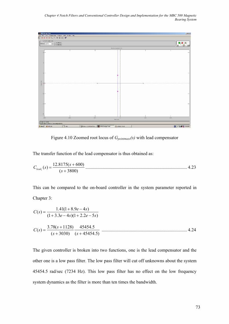
Chapter 4 Notch Filters and Conventional Controller Design and Implementation for the MBC 500 Magnetic Bearing System
73
Figure 4.10 Zoomed root locus of Gpointmass(s) with lead compensator
The transfer function of the lead compensator is thus obtained as:
)3800()600(8175.12)(
1 ++
=s
ssClead ........................................................................................ 4.23
This can be compared to the on-board controller in the system parameter reported in
Chapter 3:
)52.21)(43.31()49.81(41.1)(
sesesesC−+−+
−+=
)5.45454(5.45454
)3030()1128(78.3)(
+++
=ss
ssC .......................................................................... 4.24
The given controller is broken into two functions, one is the lead compensator and the
other one is a low pass filter. The low pass filter will cut off unknowns about the system
45454.5 rad/sec (7234 Hz). This low pass filter has no effect on the low frequency
system dynamics as the filter is more than ten times the bandwidth.

Chapter 4 Notch Filters and Conventional Controller Design and Implementation for the MBC 500 Magnetic Bearing System
74
This compensator designed should work but unfortunately when it was implemented on
the real MBC 500 magnetic bearing system, it was unsuccessful. The reason behind this
unsuccessfull implementation was the value ofα . It was observed that in order to have
the stability for the magnetic bearing system, one should not be too ambitious to provide
a large phase margin. Otherwise, it can lead to system instability. Therefore a redesign
was required.
Obtaining an Optimum α value
To overcome the above problem, the best α value needs to be determined which will
provide the optimum system stability. From the general lead compensator transfer
function equation and Clead1(s) equation shown in equations 4.17 and 4.23, the value of
α can be obtained as follows:
38001=
τ; 6001
=ατ
; 33.6600
3800600*1
===τ
α
Meanwhile, the combination of the general transfer function and the given compensator
equation is shown in equations 4.17 and 4.24 . Out of these, the value of α becomes the
following:
30301=
τ; 11281
=ατ
; 686.211283030
1128*1
===τ
α
Because of the big differences between the above two α values, the optimal value of
α needs to be determined. There must be a certain range for α that will stabilise the
system. Observing the two compensators’ bode plots shown in Figure 4.11, it is obvious
that the alpha value of Clead1(s) provides a much larger phase angle. Another point is

Chapter 4 Notch Filters and Conventional Controller Design and Implementation for the MBC 500 Magnetic Bearing System
75
that maxω (the frequency at which the phase angle is at its maximum) occurs at a lower
frequency.
Figure 4.11 Clead1(s) (solid line) and C(s) (dotted line) bode plots
Using the equations for α , a range of lead compensators were determined that
corresponded to a range of α values. For each of the compensators, there are related
variables. These related variables are the DC gain and maxω with DC gain = 1.41 (same
as DC gain for given compensator) and 7.1848max =ω rad/sec.
After calculations and lead compensator implementation on channel 1, the following
stability range for α was determined.
51 ⟨⟨α

Chapter 4 Notch Filters and Conventional Controller Design and Implementation for the MBC 500 Magnetic Bearing System
76
Therefore, for the redesign of the lead compensator for channel 2, the algebraic mean of
the range obtained for α used was 3=⇒α .
Redesign of the Lead Compensator
As determined in the previous section, 3=α and 7.1848max =ω rad/sec. Therefore, the
compensator’s zero, pole and gain values can be calculated as follows:
32021max == αω
T 3.1067
332021
==Tα 23.441.1 == zero
polexk
Therefore, the lead compensator is given by:
)3202()3.1067(23.4)(
2 ++
=s
ssClead ........................................................................................ 4.25
Moreover, the lead compensator with the low pass filter having a cut off frequency of 7
KHz incorporated is given by:
)43982(43982
)3202()3.1067(23.4)(
2 +++
=ss
ssClead ..................................................................... 4.26
This lead compensator has a DC gain of 1.41 and it also provides a phase angle of o30 .
Observing the two compensators’ bode plots in Figure 4.12, it can be seen that both of
the compensators have the peak phase at the same frequency 1849max =ω rad/sec.
Moreover, the phase angle of Clead2(s) is lower compared to the phase angle of Clead1(s)
as can be seen in Figure 4.13. Finally, a comparison of the frequency response of
Clead1(s), Clead2(s) and C(s) can be seen in Figure 4.14.

Chapter 4 Notch Filters and Conventional Controller Design and Implementation for the MBC 500 Magnetic Bearing System
77
Figure 4.12 Clead2(s) (solid line) and C(s) (dotted line) bode plots
Figure 4.13 Clead1(s) (solid line) and Clead2(s) (dotted line) bode plots

Chapter 4 Notch Filters and Conventional Controller Design and Implementation for the MBC 500 Magnetic Bearing System
78
Figure 4.14 Clead1(s) (solid line), Clead2(s) (dotted line) and C(s) (dashed line) bode plots
Digital Controller Design
Since the notch filter and lead compensator have to be implemented using DSP, it must
be transformed into digital form. The transformation from continuous time to discrete
time enables the system to be controlled through the computer with the use of
MATLAB, SIMULINK and dSPACE DSP card. A few MATLAB commands can
transform the transfer function of the continuous time controller into discrete form. The
sampling period used is 4×10⁻⁵ seconds. As a result, the sampling frequency is about ten
times the highest resonant frequency. Appendix C describes the ‘c2dm’ function, which
converts continuous linear time-invariant systems to discrete time.

Chapter 4 Notch Filters and Conventional Controller Design and Implementation for the MBC 500 Magnetic Bearing System
79
4.4 Simulation Using SIMULINK
Controller Simulation using Analytical Model
Now that the lead compensator Clead2(s) and notch filters N1(s) and N2(s) have been
designed, the whole system can be simulated using SIMULINK. The bending state-
space model will be used to represent the bearing system dynamics. The rigid body
model will not be used in the simulation as the real system does have distinct resonant
modes. Figure 4.15 shows the MATLAB SIMULINK simulation window with all the
required blocks. Note that only the x direction is taken into account, hence channel 1
and channel 2 only are included in the simulation. For channel 1, C(s) is used and
Clead2(s) for channel 2. The two outputs Vsense1 and Vsense2 can be plotted for a step input.
Figure 4.15 SIMULINK description of bending body model with controller

Chapter 4 Notch Filters and Conventional Controller Design and Implementation for the MBC 500 Magnetic Bearing System
80
For a step input of magnitude 0.001 applied to channel 1 at time t=0, the conventional
controller and the two notch filters failed to stabilise the magnetic bearing system
initially. Investigation has revealed that the two notch filters designed based on the
analytical model did not notch out the resonant at the two exact resonant frequencies.
As a result, the two notch filters have to be redesigned to cover a wide frequency range
around the two resonant frequencies. The magnetic bearing output response is given in
Figure 4.16 after the redesign of the two notch filters. Note that the system is stable with
a large overshoot to begin with.
0 0.1 0.2 0.3 0.4 0.5 0.6 0.7 0.8 0.9 1-1
0
1
2
3
4
5x 10⁻³
Time in seconds
Mag
netic
bea
ring
disp
lace
men
t out
put
Channel 1Channel 2
Figure 4.16 Step response of the magnetic bearing system-channel 1 (solid) and channel 2 (dotted)

Chapter 4 Notch Filters and Conventional Controller Design and Implementation for the MBC 500 Magnetic Bearing System
81
For input into channel 2, the result is the same, however the magnitudes are reversed.
This was the expected result as the designed conventional controllers and notch filters
stabilised both channels successfully.
Controller Simulation using the Identified Experimental Model
After the controller had been tested with the analytical model, the controller was also
tested with the identified experimental model. The experimental model that was used in
the simulation was the reduced order model Gred(s). The assumption was that if a
reasonable response was achieved, then the experimental implementation would be
successful. Figure 4.17 shows the SIMULINK block diagram containing the simplified
model obtained via system identification, the designed lead compensator and notch
filters.
A step input of magnitude 0.001 occuring at t=0 was applied for 1 second and the
response that was obtained is plotted in Figure 4.18. The horizontal scale is not in
seconds, the plot shown occurred over 0.1 seconds. Notice that the system showed
stability, and therefore it can be concluded that the designed controller should
theoretically work on the real system. The reason behind this claim is that the identified
experimental model is the closest estimate to the real system.

Chapter 4 Notch Filters and Conventional Controller Design and Implementation for the MBC 500 Magnetic Bearing System
82
Figure 4.17 SIMULINK description of the simplified model obtained via system identification with the designed compensator and notch
filters
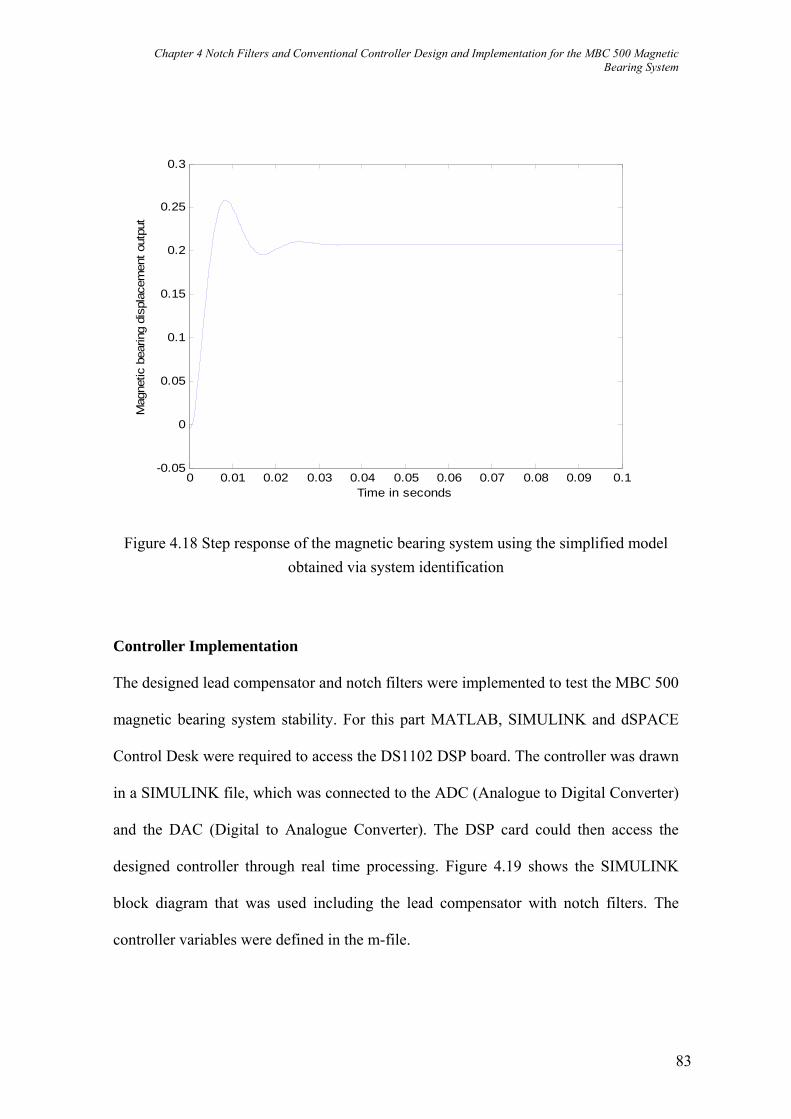
Chapter 4 Notch Filters and Conventional Controller Design and Implementation for the MBC 500 Magnetic Bearing System
83
0 0.01 0.02 0.03 0.04 0.05 0.06 0.07 0.08 0.09 0.1-0.05
0
0.05
0.1
0.15
0.2
0.25
0.3
Time in seconds
Mag
netic
bea
ring
disp
lace
men
t out
put
Figure 4.18 Step response of the magnetic bearing system using the simplified model obtained via system identification
Controller Implementation
The designed lead compensator and notch filters were implemented to test the MBC 500
magnetic bearing system stability. For this part MATLAB, SIMULINK and dSPACE
Control Desk were required to access the DS1102 DSP board. The controller was drawn
in a SIMULINK file, which was connected to the ADC (Analogue to Digital Converter)
and the DAC (Digital to Analogue Converter). The DSP card could then access the
designed controller through real time processing. Figure 4.19 shows the SIMULINK
block diagram that was used including the lead compensator with notch filters. The
controller variables were defined in the m-file.

Chapter 4 Notch Filters and Conventional Controller Design and Implementation for the MBC 500 Magnetic Bearing System
84
Figure 4.19 SIMULINK block diagram including digital controller for real time implementation
The controller designed worked for all four channels. Figure 4.20 shows the
experimental setup of the whole system in full operation. The designed digital
controllers and notch filters have been implemented using the DSP card installed in the
computer to ensure the stability of the MBC 500 magnetic bearing system. The on
screen software is MATLAB utilising the SIMULINK toolbox. The computer was
powered by a V15± DC power supply that was connected to it.

Chapter 4 Notch Filters and Conventional Controller Design and Implementation for the MBC 500 Magnetic Bearing System
85
Figure 4.20 Experimental setup of the digital control system for the MBC 500 magnetic
bearing
Figure 4.21 is an image of the MBC 500 magnetic bearing system taken while the
designed controller was stabilising channel 2. It is shown that the BNC cables were
connected to the input and output connectors of channel 2. The loop switch for channel
2 was turned off in order to disable the internal controller and all four lights indicated
the system was stable. At this stage the rotor shaft was levitating as desired.
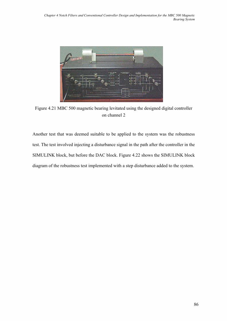
Chapter 4 Notch Filters and Conventional Controller Design and Implementation for the MBC 500 Magnetic Bearing System
86
Figure 4.21 MBC 500 magnetic bearing levitated using the designed digital controller on channel 2
Another test that was deemed suitable to be applied to the system was the robustness
test. The test involved injecting a disturbance signal in the path after the controller in the
SIMULINK block, but before the DAC block. Figure 4.22 shows the SIMULINK block
diagram of the robustness test implemented with a step disturbance added to the system.
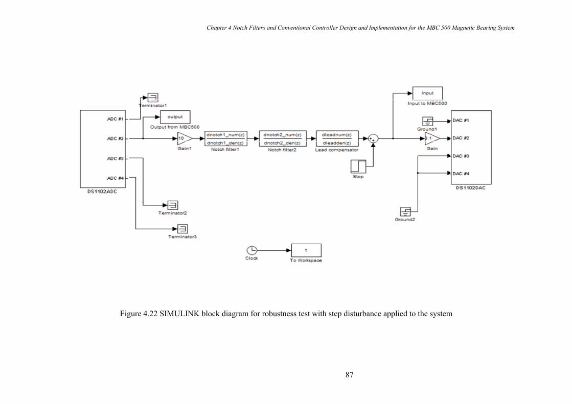
Chapter 4 Notch Filters and Conventional Controller Design and Implementation for the MBC 500 Magnetic Bearing System
87
Figure 4.22 SIMULINK block diagram for robustness test with step disturbance applied to the system

Chapter 4 Notch Filters and Conventional Controller Design and Implementation for the MBC 500 Magnetic Bearing System
88
The designed lead compensator and notch filters maintained system stability even with a
disturbance step value of 0.1 applied to the system. The system response subjected to a
step disturbance of 0.1 applied to channel 2 is given in Figure 4.23. All four channels
were tested for robustness and each test was successful.
Figure 4.23 System response subjected to a step disturbance of 0.2 applied to channel 2
The final test was to input a step signal to the input of the MBC 500 magnetic bearing
system. When the step was enforced, the movement of the rotor was observed. Figure
4.24 is the SIMULINK block diagram with the step input. The step response plot is
given in Figure 4.25.
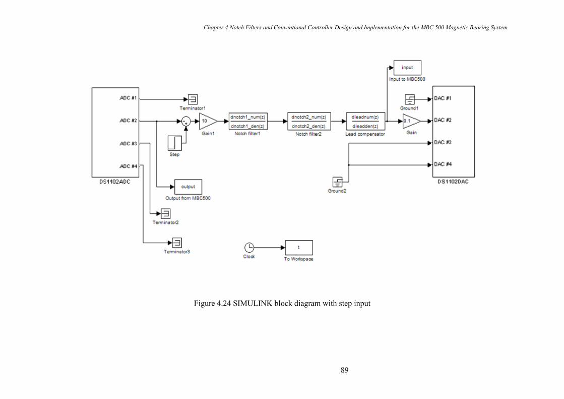
Chapter 4 Notch Filters and Conventional Controller Design and Implementation for the MBC 500 Magnetic Bearing System
89
Figure 4.24 SIMULINK block diagram with step input

Chapter 4 Notch Filters and Conventional Controller Design and Implementation for the MBC 500 Magnetic Bearing System
90
Figure 4.25 Step input response on channel 2
4.5 Summary
This chapter has described the design of notch filters based on the resonant frequencies
identified in Chapter 3. A conventional lead compensator has been designed for the
stabilisation of the magnetic bearing system. The performance of the designed notch
filters and lead compensator have been evaluated via simulation using both the
analytical model and the model obtained via system identification. The simulation
results have shown that the designed notch filters and lead compensator have stabilised
the magnetic bearing system successfully. Finally, the designed notch filters and lead
compensator have been implemented for the MBC 500 magnetic bearing system in real
time. Both the step response and robustness tests have demonstrated the effectiveness of
the conventional controller and notch filters designed.

Chapter 5 Fuzzy Logic Controller (FLC) Design for the MBC 500 Magnetic Bearing System
91
5 Fuzzy Logic Controller (FLC) Design for the MBC 500 Magnetic Bearing System
5.1 Overview
In this chapter, the structure of Fuzzy Logic Controller (FLC) is first described. Two
different fuzzy inference methods, Mamdani and Sugeno methods are then reviewed.
FLC is then designed to stabilise the MBC 500 magnetic bearing system. The
performance of the designed FLC will be evaluated via computer simulation.
Comparison studies of the FLC performance with different inference methods and
different number of rules will be investigated. Finally, this chapter presents
comparative studies of the conventional controller and the advanced PD-like Fuzzy
Logic Controller (FLC) designed that were carried out in this research.
5.2 Fuzzy Logic Controller
A block diagram of a fuzzy control system is shown in Figure 5.1. The fuzzy logic
controller is composed of four elements (Passino and Yurkovich 1998):
A rule-base, which contains a set of If-Then rules with fuzzy logic quantification
of the expert’s description, linguistically, of how to achieve good control.
An inference mechanism (an inference engine or fuzzy inference module) that
emulates how the expert makes the decision in interpreting and applying
knowledge about the best way to control the plant.

Chapter 5 Fuzzy Logic Controller (FLC) Design for the MBC 500 Magnetic Bearing System
92
A fuzzification interface, which converts controller inputs into information that
the inference mechanism can use easily to activate and apply rules.
A defuzzification interface converts the inference mechanism’s conclusions into
actual inputs for the process.
fuzz
ifica
tion
defu
zzifi
catio
n
Rule-base
Inferencemechanism
Process
Fuzzy controller
Reference inputr(t)
Inputµ(t)
Outputy(t)
Figure 5.1 Block diagram of a fuzzy controller Sources: (A Zadeh 1995; Passino and Yurkovich 1998)
In Chapter 4 it has been stated that a classical lead compensator and two notch filters
have been designed for the MBC500 magnetic bearing system. The control algorithm of
a lead compensator is equivalent to a PD controller. As a result a PD-like fuzzy
controller was designed for stabilising the MBC 500 magnetic bearing system. A block
diagram of a PD-like fuzzy control system is shown in Figure 5.2. As can be seen in
Figure 5.2, the fuzzy controller inputs are error and change-of-error. The details of the
fuzzy controller design will be shown in the following section.

Chapter 5 Fuzzy Logic Controller (FLC) Design for the MBC 500 Magnetic Bearing System
93
Figure 5.2 Block-diagram of a PD-like fuzzy control system Sources: (Reznik 1997; Passino and Yurkovich 1998)
5.3 FLC Design for AMB stabilisation
This section is focused on the design of a FLC for magnetic bearing system
stabilisation. Figure 5.3 below shows a fuzzy logic control system for one of the four
channels of the magnetic bearing system. Vsense is the sensor output of the magnetic
bearing system representing the displacement in either x or y direction. The block of
Magnetic Bearing in Figure 5.3 is composed of a power amplifier, sensor and rotor. The
FLC is designed below. The performance of the fuzzy logic control system was
investigated via simulation. The models identified in Chapter 3 were used in the
simulation.
∑
dtd
γ
Figure 5.3 FLC for MBC500 magnetic bearing system

Chapter 5 Fuzzy Logic Controller (FLC) Design for the MBC 500 Magnetic Bearing System
94
Fuzzy Logic Controller (FLC) Design
FLC Inputs and Output Selection
The inputs for the PD-like FLC are error and change-of-error. The output of the FLC is
Vcontroli that regulates the current into the bearing which in turn will regulate the
magnetic bearing force. The value of i is from 1 to 4 representing 4 channels of the
magnetic bearing. Four PD-like FLCs need to be designed for controlling the four
channels of the MBC500 magnetic system. The design of the FLC for channel x2 is
described in detail in this section. The design of the rest of the FLCs for channels x1, y1
and y2 follow the same procedure.
Figure 5.4 illustrates the MBC500 magnetic bearing shaft with the corresponding centre
reference line, and its output and input at the right hand side for channel x2.
21
2lL −
Figure 5.4 MBC 500 magnetic bearing control at right hand side for channel x2
The displacement output x2 is sensed by the Hall-effect sensor with the output voltage
Vsense2. Hence the error signal is defined for channel x2 as:
)()()( 2 tVtrte sense−=
For the magnetic bearing stabilisation problem, the reference input r(t) = 0. As a result,
)()( 2 tVte sense−=
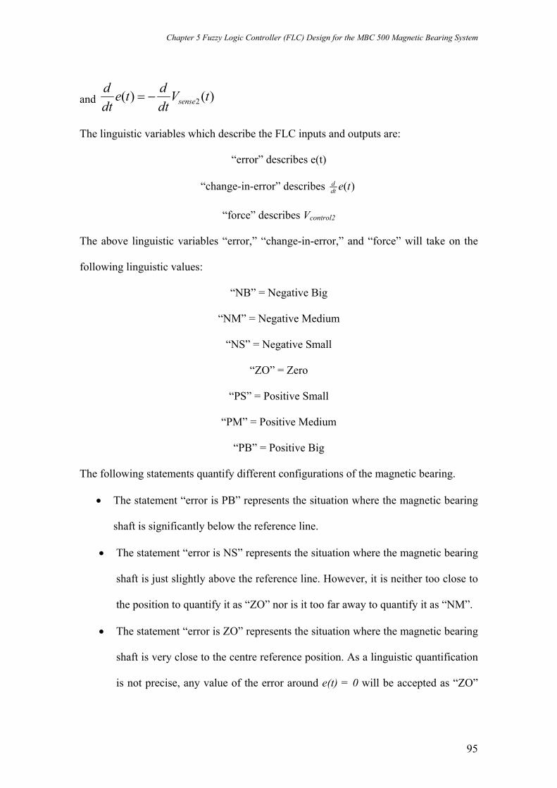
Chapter 5 Fuzzy Logic Controller (FLC) Design for the MBC 500 Magnetic Bearing System
95
and )()( 2 tVdtdte
dtd
sense−=
The linguistic variables which describe the FLC inputs and outputs are:
“error” describes e(t)
“change-in-error” describes )(tedtd
“force” describes Vcontrol2
The above linguistic variables “error,” “change-in-error,” and “force” will take on the
following linguistic values:
“NB” = Negative Big
“NM” = Negative Medium
“NS” = Negative Small
“ZO” = Zero
“PS” = Positive Small
“PM” = Positive Medium
“PB” = Positive Big
The following statements quantify different configurations of the magnetic bearing.
• The statement “error is PB” represents the situation where the magnetic bearing
shaft is significantly below the reference line.
• The statement “error is NS” represents the situation where the magnetic bearing
shaft is just slightly above the reference line. However, it is neither too close to
the position to quantify it as “ZO” nor is it too far away to quantify it as “NM”.
• The statement “error is ZO” represents the situation where the magnetic bearing
shaft is very close to the centre reference position. As a linguistic quantification
is not precise, any value of the error around e(t) = 0 will be accepted as “ZO”

Chapter 5 Fuzzy Logic Controller (FLC) Design for the MBC 500 Magnetic Bearing System
96
since this can be considered as a better quantification than “PS” or ”NS”.
• The statement “error is PB and change-in-error is PS” represents the situation
where the magnetic bearing shaft is below the reference line and, since
02 <sensedtd V , the magnetic bearing shaft is moving away from the centre
position.
• The statement “error is NS and change-in-error is PS” represents the situation
where the magnetic bearing shaft is slightly above the centre reference line and,
since 02 <sensedtd V , the magnetic bearing shaft is moving toward the centre
position.
Rule-Base Formulation
The above linguistic quantification would be used to specify a set of rules or a rule-base.
The following three situations will demonstrate how the rule-base is developed.
1. If error is NB and change-in-error is NB Then force is NB.
Figure 5.5 below shows that the magnetic bearing shaft at the right end has a large
displacement and is moving up away from the centre reference line. Therefore, it is
clear that a strong negative force should be applied so that the shaft will move to the
centre reference position.
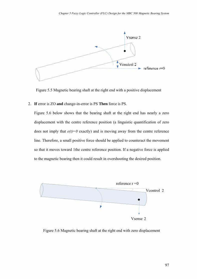
Chapter 5 Fuzzy Logic Controller (FLC) Design for the MBC 500 Magnetic Bearing System
97
Figure 5.5 Magnetic bearing shaft at the right end with a positive displacement
2. If error is ZO and change-in-error is PS Then force is PS.
Figure 5.6 below shows that the bearing shaft at the right end has nearly a zero
displacement with the centre reference position (a linguistic quantification of zero
does not imply that e(t)=0 exactly) and is moving away from the centre reference
line. Therefore, a small positive force should be applied to counteract the movement
so that it moves toward 1the centre reference position. If a negative force is applied
to the magnetic bearing then it could result in overshooting the desired position.
Vsense 2
Vcontrol 2
reference r =0
Figure 5.6 Magnetic bearing shaft at the right end with zero displacement

Chapter 5 Fuzzy Logic Controller (FLC) Design for the MBC 500 Magnetic Bearing System
98
3. If error is PB and change-in-error is NS Then force is PS.
Figure 5.7 below shows that the bearing shaft at the right end is far below the centre
reference line and is moving towards the centre reference position. Therefore, a
small positive force should be applied to assist the movement. However, it should
not be a big force since the bearing shaft at the right end is already moving in the
proper direction.
Figure 5.7 Magnetic bearing shaft at the right end with a negative displacement
Following a similar analysis, the rules of the FLC for controlling the magnetic bearing
shaft can be developed. For the FLC with two inputs and five linguistic values for each
input, there are 2555 = possible rules with all combination for the inputs. Similarly, for
the FLC with two inputs and seven linguistic values for each input, there are 4972 =
possible rules with all combination for the inputs. A set of possible linguistic values for
two inputs and one output with 25 rules are NB, NS, ZO, PS and PB. Furthermore, A
set of possible linguistic values for two inputs and one output with 49 rules are NB,
NM, NS, ZO, PS, PM and PB. One way to list all possible rules where inputs are less
than or equal to two or three is by using a tabular representation. The tabular
representations of the FLC rule base (25 rules and 49 rules) of the magnetic bearing

Chapter 5 Fuzzy Logic Controller (FLC) Design for the MBC 500 Magnetic Bearing System
99
fuzzy control system are shown in Tables 5.1 and 5.2 respectively.
“force” “change-in-error” •
e
V NB NS ZO PS PB
NB NB NB NB NS ZO
NS NB NB NS ZO PS
ZO NB NS ZO PS PM
PS NS ZO PS PB PB
“error”
e
PB ZO PS PB PB PB
Table 5.1 Rule table with 25 rules
“force” “change-in-error”
ė V NB NM NS ZO PS PM PB
NB NB NB NB NB NM NS ZO NM NB NB NB NM NS ZO PS NS NB NB NM NS ZO PS PM ZO NB NM NS ZO PS PM PB PS NM NS ZO PS PM PB PB PM NS ZO PS PM PB PB PB
“error” e
PB ZO PS PM PB PB PB PB Table 5.2 Rule table with 49 rules
The body of the FLC rule tables shown above lists the linguistic-numeric consequents.
The left column and top row of the table contain the linguistic-numeric terms of the
inputs. Tables 5.1 and 5.2 present abstract knowledge that the expert has about how to
control the magnetic bearing shaft’s given error and its derivative as inputs. All those
rules have been determined to be complete, consistent and continuous.

Chapter 5 Fuzzy Logic Controller (FLC) Design for the MBC 500 Magnetic Bearing System
100
Fuzziffication (Fuzzy Quantification of Knowledge)
Up to now, linguistic values have been used to describe the inputs and output of the
FLC to specify a set of rules (a rule-base) about how to control the plant. The meaning
of these linguistic values is quantified using membership functions. Figure 5.8 shows
the FLC constructed using MATLAB’s fuzzy logic toolbox with inputs “error” and
“change-of-error” and the output “force”. The input “change-of-error” has been
quantified using the triangular memberships as shown in the figure. The membership
functions for “error” and the output “force” have been defined using similar
membership functions in a normalised universe of discourse [-1,1].
Figure 5.8 Membership functions for the input “change-of-error” in a normalised universe of discourse

Chapter 5 Fuzzy Logic Controller (FLC) Design for the MBC 500 Magnetic Bearing System
101
Different types of membership functions have been chosen, different methods for fuzzy
intersection (t-norm) and union (s-norm), different numbers of rules (25 rules and 49
rules), and different fuzzy inference methods have been investigated to explore the
effectiveness of the designed FLC.
Simulation Results
The transfer function of the magnetic bearing model obtained via system identification,
shown previously in Chapter 3, was used here in the simulation and the transfer function
is repeated below:
5.8e020 - s 1.086e018 s^2 3.881e015 s^3 5.897e010 s^4 1.899e008 s^5 334.6 s^67.938e020 s 3.814e017 - s^2 6.086e013 s^3 1.961e010 - s^4 4.038e005 s^5 105.2-)(
++++++++
=sG
Figure 5.9 shows the SIMULINK block diagram of the magnetic bearing system with
the designed FLC. In contrast to the conventional control approach which has two notch
filters taking care of the two resonant modes, the two notch filters are not present in the
fuzzy control approach. Using notch filters designed as reported in Chapter 4, a
sampling frequency of fs=25 kHz was used when implementing the conventional
controller and notch filters. As a result a delay time of 4×10⁻⁵ seconds was chosen for
the unit delay which was used to calculate the change-of-error signal.

Chapter 5 Fuzzy Logic Controller (FLC) Design for the MBC 500 Magnetic Bearing System
102
Figure 5.9 SIMULINK block diagram of the magnetic bearing system with the designed FLC
Different membership functions, such as the triangular and Gaussian membership
functions, have been used for the FLC. The effect of using different methods for fuzzy
intersections (t-norm) and unions (s-norm) have been investigated. Both Mamdani and
Sugeno inference methods have been studied. Thus, four typical methods have been
investigated with four cases in each method.
Some of the concepts used in MATLAB’s Fuzzy Logic Toolbox are repeated here to
avoid any confusion. Aggregation refers to the methods of determining the combination
of the consequents of each rule in a Mamdani fuzzy inference system in preparation for
defuzzification. Implication refers to the process of shaping the fuzzy set in the
consequent based on the results of the antecedent in a Mamdani-type fuzzy inference
system. In the MATLAB fuzzy logic toolbox, two built in t-norm (AND) operations are
supported: MIN (minimum) and PROD (product). Two built in s-norm (OR) operations
are supported: MAX (maximum) and probabilistic OR method PROBOR. The
probabilistic OR method is calculated according to the following equation:

Chapter 5 Fuzzy Logic Controller (FLC) Design for the MBC 500 Magnetic Bearing System
103
PROBOR (a,b) = a + b –ab
Method 1: FLC with 25 Rules Using Mamdani Inference Method
Case 1
In the first case, the designed FLC uses triangular membership functions for the inputs
and output. The FLC uses MIN for t-norm operation, MAX for s-norm operation, MAX
for aggregation, MIN for implication, and CENTROID for defuzzification.
Case 2
In the second case, the designed FLC uses triangular membership functions for the
inputs and output. The FLC uses PROD for t-norm operation, PROBOR for s-norm
operation, MAX for aggregation, PROD for implication, and CENTROID for
defuzzification.
Case 3
In the third case, the designed FLC uses Gaussian membership functions for both inputs
and output. The FLC also uses MIN for t-norm operation, MAX for s-norm operation,
MAX for aggregation, MIN for implication, and CENTROID for defuzzification.
However, the FLC failed to stabilise the magnetic bearing system in this case.
Case 4
In the last case, the designed FLC uses Gaussian membership functions for both inputs
and output. The FLC also uses PROD for t-norm operation, PROBOR for s-norm
operation, MAX for aggregation, PROD for implication, and CENTROID for
defuzzification.

Chapter 5 Fuzzy Logic Controller (FLC) Design for the MBC 500 Magnetic Bearing System
104
Figure 5.10 shows the step responses of the magnetic bearing system with the designed
FLCs for the four cases described above. It can be seen that the system is stable with the
FLCs in cases 1, 2 and 4. The FLC in case 3 failed to stabilise the magnetic bearing
system. The step responses with the FLCs in cases 2 and 4 have less damping and
longer settling time than case 1. From the step responses shown in this figure, it can be
seen that the FLC in case 1 provides the best result. However, all results exhibit a large
steady-state error as the reference step size is 0.1.
0 0.01 0.02 0.03 0.04 0.05 0.06 0.07 0.08 0.09 0.1-0.1
0
0.1
0.2
0.3
0.4
0.5
0.6
Time in seconds
Mag
netic
bea
ring
disp
lace
men
t out
put
25-rule FLC with Mamdani inference method
Case 1Case 2Case 4
Figure 5.10 Step response of the magnetic bearing system with the designed FLC (25 rules, Mamdani inference method)
Method 2: FLC with 49 Rules Using Mamdani Inference Method
Figure 5.11 shows the step responses of the magnetic bearing system with the designed
49-rule FLC for the same four cases described in method 1. Comparing the simulation
results in these figures, it can be seen that the FLC used in case 1 provides the step

Chapter 5 Fuzzy Logic Controller (FLC) Design for the MBC 500 Magnetic Bearing System
105
response with the smallest overshoot. The FLC in case 2 provides the step response with
the smallest steady-state error. The FLC in case 1 provides the best step response in
terms of overall performance. Again, all results exhibit a large steady-state error as the
reference step size is 0.1.
0 0.01 0.02 0.03 0.04 0.05 0.06 0.07 0.08 0.09 0.1-0.1
0
0.1
0.2
0.3
0.4
0.5
0.6
0.7
Time in seconds
Mag
netic
bea
ring
disp
lace
men
t out
put
49-rule FLC with Mamdani inference method
Case 1Case 2Case 3Case 4
Figure 5.11 Step response of the magnetic baring system with the designed FLC
(49 rules, Mamdani inference method)
Method 3: 25-rule FLC with Sugeno Fuzzy Inference Method
Case 1
In the first case, the designed FLC uses triangular membership functions for the inputs
and output. The FLC also uses MIN for t-norm operation, MAX for s-norm operation,
and the WTAVER (weighted average) is the defuzzification method used.

Chapter 5 Fuzzy Logic Controller (FLC) Design for the MBC 500 Magnetic Bearing System
106
Case 2
In the second case, the designed FLC uses triangular membership functions for the
inputs and output. The FLC uses PROD for t-norm operation, MAX for s-norm
operation, and WTAVER for defuzzification.
Case 3
In the third case, the designed FLC uses Gaussian membership functions for both inputs
and output. The FLC also uses MIN for t-norm operation, MAX for s-norm operation,
and WTAVER for defuzzification.
Case 4
In the last case, the designed FLC uses Gaussian membership functions for both inputs
and output. The FLC also uses PROD for t-norm operation, MAX for s-norm operation,
and WTAVER for defuzzification.
Figure 5.12 shows the step responses of the magnetic bearing system with the designed
FLCs for the four cases described above. It can be seen that the system is stable and
there is not much of difference in terms of steady-state error. The step response with the
FLC in case 1 provides the best result as it has more damping and faster settling time.
However, all results exhibit a large steady-state error as the reference step size is 0.1.

Chapter 5 Fuzzy Logic Controller (FLC) Design for the MBC 500 Magnetic Bearing System
107
0 0.01 0.02 0.03 0.04 0.05 0.06 0.07 0.08 0.09 0.1-0.1
0
0.1
0.2
0.3
0.4
0.5
0.6
Time in seconds
Mag
netic
bea
ring
disp
lace
men
t out
put
25-rule FLC with Sugeno inference method
Case 1Case 2Case 3Case 4
Figure 5.12 Step response of the magnetic bearing system with the designed FLC (25 rules, Sugeno inference method)
Method 4: 49-rule FLC with Sugeno Fuzzy Inference Method
Figure 5.13 shows the step responses of the magnetic bearing system with the designed
FLCs for the the same four cases described in method 3. Comparing the simulation
results in this figure, it can be seen that the FLC in case 1 provides the result with the
most damping and faster settling time. Again, all results exhibit a large steady-state
error as the reference step size is 0.1.
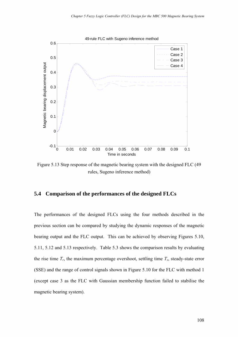
Chapter 5 Fuzzy Logic Controller (FLC) Design for the MBC 500 Magnetic Bearing System
108
0 0.01 0.02 0.03 0.04 0.05 0.06 0.07 0.08 0.09 0.1-0.1
0
0.1
0.2
0.3
0.4
0.5
0.6
Time in seconds
Mag
netic
bea
ring
disp
lace
men
t out
put
49-rule FLC with Sugeno inference method
Case 1Case 2Case 3Case 4
Figure 5.13 Step response of the magnetic bearing system with the designed FLC (49
rules, Sugeno inference method)
5.4 Comparison of the performances of the designed FLCs
The performances of the designed FLCs using the four methods described in the
previous section can be compared by studying the dynamic responses of the magnetic
bearing output and the FLC output. This can be achieved by observing Figures 5.10,
5.11, 5.12 and 5.13 respectively. Table 5.3 shows the comparison results by evaluating
the rise time Tr, the maximum percentage overshoot, settling time Ts, steady-state error
(SSE) and the range of control signals shown in Figure 5.10 for the FLC with method 1
(except case 3 as the FLC with Gaussian membership function failed to stabilise the
magnetic bearing system).

Chapter 5 Fuzzy Logic Controller (FLC) Design for the MBC 500 Magnetic Bearing System
109
Tr Overshoot Ts SSE Control signal range
Case 1 0.011 16.4% 0.056 -0.32 -0.368 to 0.138 Case 2 0.01 30.9% 0.05 -0.263 -0.392 to 0.09 Case 3 N/A N/A N/A N/A N/A Case 4 0.01 36.7% 0.056 -0.273 -0.439 to 0.057
Table 5.3 Performance comparison of the designed FLC with method 1 It can be seen that the designed FLC in case 1 uses the triangular membership functions
for the inputs and output, MIN for t-norm operation, MAX for s-norm operation, MIN
for implication, and CENTROID for defuzzification gave the best result among others.
Table 5.4 shows the comparison results by evaluating the rise time Tr, the maximum
percentage overshoot, settling time Ts, steady-state error (SSE) and the range of control
signals shown in Figure 5.11 for the FLC with method 2.
Tr Overshoot Ts SSE Control signal range Case 1 0.012 12.4% 0.03 -0.312 -0.37 to 0.24 Case 2 0.01 38.05% 0.046 -0.24 -0.35 to 0.15 Case 3 0.015 12.23% 0.04 -0.45 -0.47 to 0.2 Case 4 0.022 2.1% 0.03 -0.435 -0.4 to 0.1
Table 5.4 Performance comparison of the designed FLC with method 2
It can be seen from Table 5.4 that the FLC uses triangular membership functions for the
inputs and outputs, MIN for t-norm operation, MAX for s-norm operation, MAX for
aggregation, MIN for implication, and CENTROID for defuzzification (case 1)
provides the best result in terms of overshoot, settling time and steady state error.
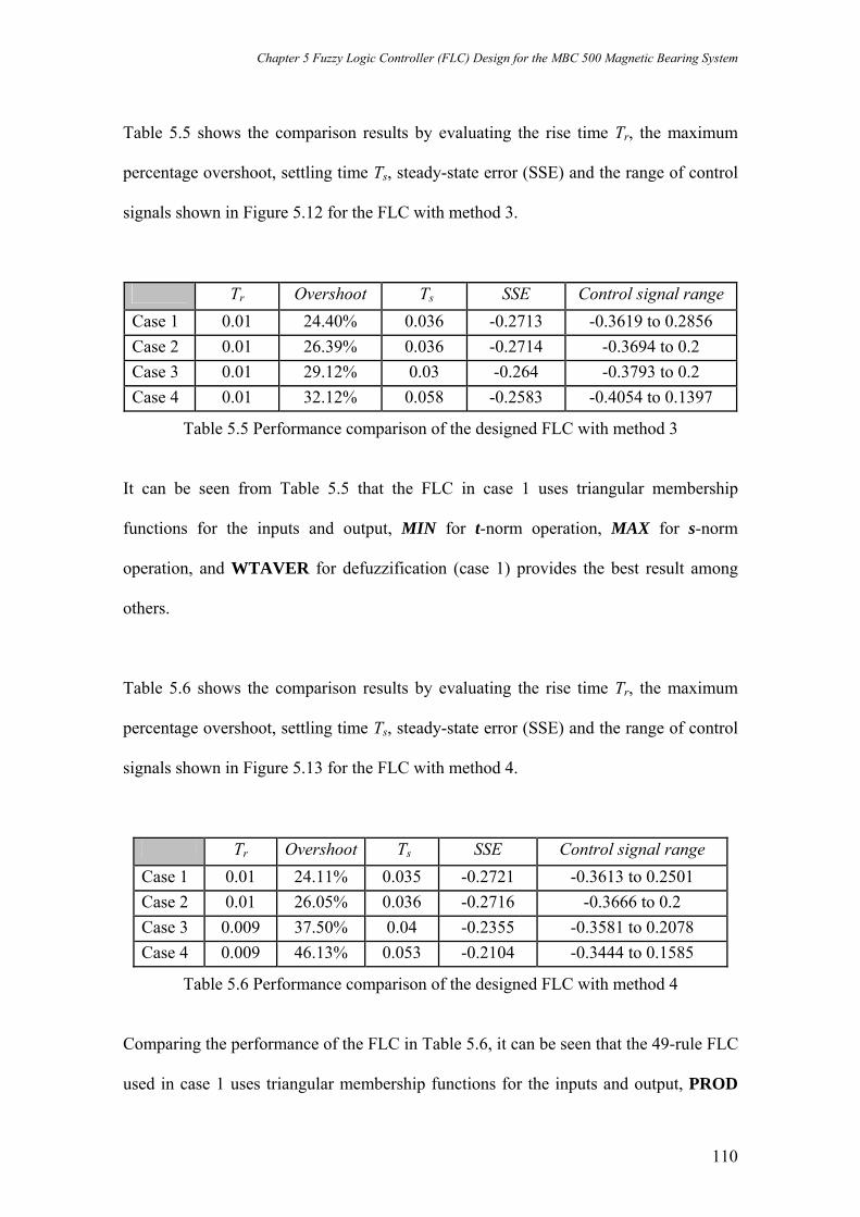
Chapter 5 Fuzzy Logic Controller (FLC) Design for the MBC 500 Magnetic Bearing System
110
Table 5.5 shows the comparison results by evaluating the rise time Tr, the maximum
percentage overshoot, settling time Ts, steady-state error (SSE) and the range of control
signals shown in Figure 5.12 for the FLC with method 3.
Tr Overshoot Ts SSE Control signal range Case 1 0.01 24.40% 0.036 -0.2713 -0.3619 to 0.2856 Case 2 0.01 26.39% 0.036 -0.2714 -0.3694 to 0.2 Case 3 0.01 29.12% 0.03 -0.264 -0.3793 to 0.2 Case 4 0.01 32.12% 0.058 -0.2583 -0.4054 to 0.1397
Table 5.5 Performance comparison of the designed FLC with method 3
It can be seen from Table 5.5 that the FLC in case 1 uses triangular membership
functions for the inputs and output, MIN for t-norm operation, MAX for s-norm
operation, and WTAVER for defuzzification (case 1) provides the best result among
others.
Table 5.6 shows the comparison results by evaluating the rise time Tr, the maximum
percentage overshoot, settling time Ts, steady-state error (SSE) and the range of control
signals shown in Figure 5.13 for the FLC with method 4.
Tr Overshoot Ts SSE Control signal range Case 1 0.01 24.11% 0.035 -0.2721 -0.3613 to 0.2501 Case 2 0.01 26.05% 0.036 -0.2716 -0.3666 to 0.2 Case 3 0.009 37.50% 0.04 -0.2355 -0.3581 to 0.2078 Case 4 0.009 46.13% 0.053 -0.2104 -0.3444 to 0.1585
Table 5.6 Performance comparison of the designed FLC with method 4
Comparing the performance of the FLC in Table 5.6, it can be seen that the 49-rule FLC
used in case 1 uses triangular membership functions for the inputs and output, PROD

Chapter 5 Fuzzy Logic Controller (FLC) Design for the MBC 500 Magnetic Bearing System
111
for t-norm operation, MAX for s-norm operation, and WTAVER for defuzzification
provides the best result.
Figure 5.14 shows the four best step responses of the magnetic bearing system under
fuzzy logic control using the four methods, respectively. The solid line shows the best
response of the magnetic bearing system using the 25-rule FLC with Mamdani inference
method. The dotted line illustrates the best response of the magnetic bearing system
using the 25-rule FLC with the Sugeno inference method. The dash-dotted line is the
best response of the magnetic bearing system using the 49-rule FLC with the Mamdani
inference method and the dashed line provides the best response of the magnetic bearing
system using the 49-rule FLC with the Sugeno inference method.
0 0.01 0.02 0.03 0.04 0.05 0.06 0.07 0.08 0.09 0.1-0.1
0
0.1
0.2
0.3
0.4
0.5
0.6
Time in seconds
Mag
netic
bea
ring
disp
lace
men
t out
put
Method 1-25-rule FLC with Mamdani inference methodMethod 3 - 25-rule FLC with Sugeno inference method Method 2 - 49-rule FLC with Mamdani inference methodMethod 4 - 49-rule FLC with Sugeno inference method
Figure 5.14 Comparison of the best step responses of the magnetic bearing control system with the FLC designed using the four methods

Chapter 5 Fuzzy Logic Controller (FLC) Design for the MBC 500 Magnetic Bearing System
112
From Figure 5.14 it can be seen that method 2 provides the best result as it leads to a
quicker and well damped response.
Investigation of Different Deffuzification Methods
Further studies have been carried out by investigating the effect of different
defuzzification methods. The following methods are provided in the MATLAB fuzzy
logic toolbox: the centroid of area method (centre of gravity), the bisector of area
method, the mean of maximum method, the smallest of maximum method, and the
largest of maximum method. All methods have been investigated and it is found that the
centroid of area method provides the best simulation result.
Tuning via Scaling the Input and Output Universes of Discourses
The simulation results shown previously all have a large steady-state error. This error
cannot be completely eliminated as the controller designed is a PD-like FLC which
doesn’t have integration property. However, the output response can be improved by
adjusting the scaling factors Kp, Kd and h shown in Figure 5.9. This in turn will adjust
the universe of discourses for the input and output membership functions. Figure 5.15
shows a comparison result with different scaling factors. It can be seen that the steady-
state error has been reduced dramatically with Kp=1, Kd=1 and h=2. However, the
damping on the step response has been reduced. The response with Kp=1, Kd=1 and
h=1.4 provides the result with a small steady-error and faster settling time.
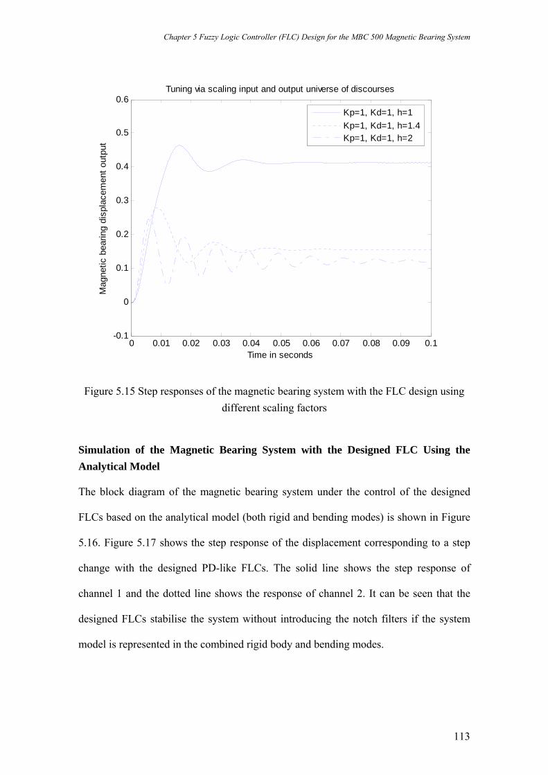
Chapter 5 Fuzzy Logic Controller (FLC) Design for the MBC 500 Magnetic Bearing System
113
0 0.01 0.02 0.03 0.04 0.05 0.06 0.07 0.08 0.09 0.1-0.1
0
0.1
0.2
0.3
0.4
0.5
0.6
Time in seconds
Mag
netic
bea
ring
disp
lace
men
t out
put
Tuning via scaling input and output universe of discourses
Kp=1, Kd=1, h=1Kp=1, Kd=1, h=1.4Kp=1, Kd=1, h=2
Figure 5.15 Step responses of the magnetic bearing system with the FLC design using different scaling factors
Simulation of the Magnetic Bearing System with the Designed FLC Using the Analytical Model The block diagram of the magnetic bearing system under the control of the designed
FLCs based on the analytical model (both rigid and bending modes) is shown in Figure
5.16. Figure 5.17 shows the step response of the displacement corresponding to a step
change with the designed PD-like FLCs. The solid line shows the step response of
channel 1 and the dotted line shows the response of channel 2. It can be seen that the
designed FLCs stabilise the system without introducing the notch filters if the system
model is represented in the combined rigid body and bending modes.
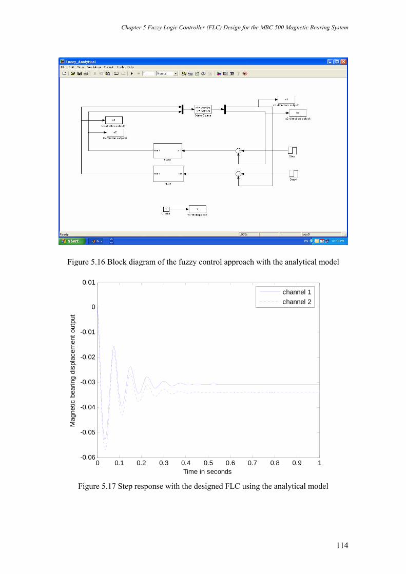
Chapter 5 Fuzzy Logic Controller (FLC) Design for the MBC 500 Magnetic Bearing System
114
Figure 5.16 Block diagram of the fuzzy control approach with the analytical model
0 0.1 0.2 0.3 0.4 0.5 0.6 0.7 0.8 0.9 1-0.06
-0.05
-0.04
-0.03
-0.02
-0.01
0
0.01
Time in seconds
Mag
netic
bea
ring
disp
lace
men
t out
put
channel 1channel 2
Figure 5.17 Step response with the designed FLC using the analytical model

Chapter 5 Fuzzy Logic Controller (FLC) Design for the MBC 500 Magnetic Bearing System
115
Implementation of the FLC Designed for the MBC 500 Magnetic Bearing System
The FLC was programmed in C language. The sampling period used in the
implementation is 4×10⁻⁵ seconds. However, it was found that the DSP was unable to
execute all the code in the specified sample period. One solution to this problem is to
program the FLC using Assembler language. The other alternative is to purchase a
much faster DSP card. However, due to time and financial constraints, these alternatives
could not be explored in this research; these have been left as further work to be carried
out at a later stage.
5.5 Comparison between the Conventional Controller and the Advanced Fuzzy Logic Controller (FLC) for Magnetic Bearing Stabilisation
Conventional Controller
It was demonstrated previously in Chapter 4 that there were two resonant modes which
threaten the stability of the closed loop magnetic bearing system. The conventional lead
compensator cannot handle the two dominant resonant modes of the magnetic bearing
system. This necessitates the design of two notch filters to filter out the unwanted
characteristics at the resonant frequencies. From the analytical and experimental models
of the MBC500 magnetic bearing system, it was found that the two resonant modes are
located at approximately 749 Hz and 2069 Hz. After two notch filters were designed to
handle the two resonant modes, a lead compensator was designed to stabilise the
magnetic bearing system. The lead compensator added a positive phase to the system in
a given frequency range. The compensator design was based on the analytical rigid
body model where the shaft was a point mass with no angle variable ө.
Chapter 5 Fuzzy Logic Controller (FLC) Design for the MBC 500 Magnetic Bearing System
116
The performances of the conventional lead compensator and the two notch filters
designed have been evaluated via simulation using both the analytical model and the
model obtained via system identification. The designed lead compensator and notch
filters were also implemented in real time for the MBC 500 magnetic bearing system.
The controller designed worked for all four channels of the MBC 500 magnetic bearing
system. Tests were performed to test the dynamic response and robustness of the
conventional controller and the notch filter designed and each test was successful.
Advanced Fuzzy Logic Controller (FLC)
A PD-like FLC was designed for stabilising the magnetic bearing system. Two different
numbers of rule sets (25-rule and 49-rule) were formulated for the PD-like FLC. Two
different fuzzy inference methods, the Mamdani and Sugeno methods, have been used.
The performance of the designed FLC has been evaluated via simulation. Comparison
studies of the FLC performances with two different sets of rules, two different inference
methods, different membership functions, different t-norm and s-norm operations, and
different defuzzification methods have been investigated. Simulation results show that
the FLC designed leads to a good system performance. To further improve system
performance, scaling factors have been tuned. Simulation has also been carried out
based on the analytical model derived that represented both the rigid body and bending
modes. Again, simulations have shown highly promising results.
The simulation performance showed that the FLC designed can handle the resonant
modes very well without the presence of the two notch filters.
Based on all the simulation results reported above, it was concluded that the designed
49-rule FLC uses triangular membership functions for the inputs and output, MIN for t-

Chapter 5 Fuzzy Logic Controller (FLC) Design for the MBC 500 Magnetic Bearing System
117
norm operation, MAX for s-norm operation, MAX for aggregation, MIN for
implication, and CENTROID for defuzzification provides the best result.
0 0.01 0.02 0.03 0.04 0.05 0.06 0.07 0.08 0.09 0.1-0.05
0
0.05
0.1
0.15
0.2
0.25
0.3
Time in seconds
Mag
netic
bea
ring
disp
lace
men
t out
put
Conventional controller with two notch filtersFLC without notch filters
Figure 5.18 Comparison results of the step response of the magnetic bearing system with the designed conventional controller and the designed FLC
Figure 5.18 shows the step response of the magnetic bearing system with the designed
conventional controller and the designed FLC based on the identified model of the
MBC 500 magnetic bearing system. Comparing the simulation results of the
conventional controller and the advanced PD-like FLC, it can be seen that the response
with the designed conventional controller has less settling time. The step response with
the designed advanced PD-like FLC has longer setting time but less steady-state error.
Moreover, the advanced PD-FLC can handle the two resonant modes without the need
of using the two notch filters.

Chapter 5 Fuzzy Logic Controller (FLC) Design for the MBC 500 Magnetic Bearing System
118
5.6 Summary
This chapter started with the structure of a basic FLC. Two different fuzzy inference
methods, the Mamdani and Sugeno methods, have been reviewed. The process of
developing and designing the FLC for the stabilisation of the magnetic bearing system
has been described. The performance of the designed FLC has been evaluated via
simulation. The simulation result shows that the FLC designed leads to a good system
performance. Comparison studies of the FLC performances with two different sets of
rules, two different inference methods, different membership functions, different t-norm
and s-norm operations, and different defuzzification methods have been investigated. To
further improve system performance, scaling factors have been tuned. Again,
simulations have shown highly promising results.
Finally, this chapter has compared the controller simulation for both the conventional
controller and advanced PD-like fuzzy logic controller via evaluating controller
performance. The advantage of using the conventional controller lies in its simplicity
for real-time implementation. The disadvantage of using the conventional controller is
that it cannot handle the resonant modes and as a result additional notch filters are
needed in this method. If the notch filters are not designed properly, they can lead to the
instability of the system. In addition, four separate conventional controllers were
designed, based on the four models of the four channels of the magnetic bearing system.
The first advantage of the PD-like FLC is that it can handle the resonant modes well
without using notch filters. As a result, this will not threaten the stability of the system.
The second advantage of the PD-like FLC is that as the FLC is nonlinear, the PD-like
FLC designed for one channel should work for all other three channels. However, the
PD-like FLCs are more computationally intensive than the conventional controller. Due

Chapter 5 Fuzzy Logic Controller (FLC) Design for the MBC 500 Magnetic Bearing System
119
to the speed limit of the DS1102 DSP card, the PD-like FLC cannot be implemented at
this stage. The overall conclusion and direction for future development will be
discussed in the next chapter.

Chapter 6 Conclusion and Future Work
120
6 Conclusion and Future Work
6.1 Overview
In this last chapter, all the preceding chapters will be brought together with the aim to
examine the extent to which the objectives have been achieved. This chapter also will
present some directions for future development and other related work.
6.2 General Conclusion
The study has investigated the techniques for identifying a system model and designing
both the conventional and advanced controllers for Active Magnetic Bearing (AMB)
system stabilisation.
In Chapter 3 it has been reported that an analytical model of the MBC 500 magnetic
bearing system has been derived. This provided the basic knowledge of the AMB
system’s rigid body and bending body models. In the same Chapter 3 it has been
reported that a model has been obtained via a two-step closed-loop system
identification. This research concludes that the magnetic bearing system is complex to
model both analytically and experimentally. Although complex, the analytical model
has provided a realistic view of the real system. The model obtained via system
identification has provided adequate information on the low frequency and the two
resonant modes of the MBC 500 magnetic bearing system.

Chapter 6 Conclusion and Future Work
121
In Chapter 4 the design of notch filters based on the resonant frequencies as reported in
Chapter 3 has been carried out. The two notch filters have been designed in order to
control the magnitude and phase fluctuations at the resonant modes in the system. A
conventional controller has been designed and implemented based on the model
obtained as reported in Chapter 4. A significant conclusion has been drawn when
designing the lead compensator. It has been found that a controller with too large a
positive phase angle has a negative effect on the magnetic bearing system. This finding
is very significant because it restricts the controller design specifications and yields an
optimum lead angle for the compensator. The performance of the designed controller
and the two notch filters have been evaluated via computer simulation using MATLAB
and SIMULINK. This conventional controller and the two notch filters have also been
implemented using the dSPACE DS1102 DSP card.
In Chapter 5 the Fuzzy Logic theory and Fuzzy Logic Controller (FLC) structures with
two different fuzzy inference methods that this study has drawn upon have been
reported. These inference methods are Mamdani and Sugeno-Type fuzzy inference
methods. PD-like FLC has then been designed for the AMB system stabilisation. Two
different numbers of rule sets (25-rule and 49-rule) were formulated for the PD-like
FLC. Two different fuzzy inference methods, Mamdani and Sugeno methods, have been
used. The performance of the designed FLC has been evaluated via simulation.
Comparison studies of the FLC performances with two different sets of rules, two
different inference methods, different membership functions, different t-norm and s-
norm operations, and different defuzzification methods have been investigated. The
simulation result showed that the FLC designed leads to a good system performance. To

Chapter 6 Conclusion and Future Work
122
further improve system performance, scaling factors have been tuned. Again,
simulations based on both the identified model and the analytical models of the
MBC500 magnetic bearing system have shown highly promising results. It must be
pointed out that the simulation performance has shown that the FLC designed can
handle the resonant modes very well without the presence of the two notch filters.
Comparison studies of the designed conventional and the advanced PD-like FLC for the
AMB system stabilisation have been evaluated via controller performance simulation.
This has been reported in chapter 5. The simulation results have shown that both the
conventional and the advanced PD-like FLC stabilise the MBC 500 magnetic bearing
system successfully. The advantage of using the conventional controller lies in its
simplicity for real-time implementation. The disadvantage of using the conventional
controller is that it cannot handle the resonant modes and as a result additional notch
filters are needed in this method. If the notch filters are not designed properly, it can
lead to the instability of the system. The first advantage of the PD-like FLC is that it can
handle the resonant modes well without using notch filters. As a result, this will not
threaten the stability of the system. The second advantage of the PD-like FLC is that as
the FLC is nonlinear, the PD-like FLC designed for one channel should work for all
other three channels. However, the PD-like FLC are more computationally intensive
than the conventional controller. Due to the speed limit of the DS1102 DSP card, the
PD-like FLC cannot be implemented at this stage.
Chapter 6 Conclusion and Future Work
123
6.3 Suggestions for Future Research
The extensions of this research lie primarily in the areas of implementation and
applications of the FLC. It is highly recommended that a faster DSP be used for the
implementation of the FLC.
The rotor in the MBC 500 magnetic bearing system has been suspended but is not
rotating. In magnetic bearings the shafts (rotors) are often required to rotate at high
speeds and unbalanced masses in these systems generate significant disturbance forces
called synchronous forces. The synchronous forces cause vibration of the rotors and can
often lead to severe problems in rotating machines. Another extension of the research is
to investigate both conventional and advanced approaches for attenuating the effects of
synchronous disturbances in the magnetic bearing systems.

124
Bibliography
Designing Lead and Lag Compensator. Control Tutorials for Matlab, The University of Michigan. 2005.
A Zadeh, L. (1995). Fuzzy Logic Toolbox. Release Notes for Release 14 with Service Pack 1. Berkeley, CA.
Allaire, P. E., D. W. Lewis, et al. (1981). "Feedback Control of a Single Mass Rotor on Rigid Supports." J. Franklin Inst. 312(1): pp.1-11.
Allaire, P. E., D. W. Lewis, et al. (1983). "Active Vibration Control of a Single Mass Rotor of Flexible Supports." J.Franklin Inst 315(3): pp.211-222.
Balas, G. J., J. C. Doyle, et al. (1995). Matlab µ-Analysis and Synthesis Toolbox. Natick, MA, USA, The Mathworks.
Bleuler, H., C. Gahler, et al. (1994). "Application of Digital Signal Processors for Industrial Magnetic Bearings." IEEE Trans. Control System Technology 2(4): pp.280-289.
Chen, M. and C. L. Knospe (2005). "Feedback Linearization of Active Magnetic Bearings: Current-Mode Implementation." IEEE/ASME Transaction On Mechatronics 10(6): pp.632-639.
Dorf, R. C. and R. H. Bishop (1995). Modern Control Systems, Addison-Wesley Publishing Company.
Fujita, M., F. Matsumura, et al. (1990). Experiments on the H Disturbances Attenuation Control of A Magnetic Suspension System. Proc of the 29 th IEEE Conference Decision and Control.
Habib, M. M. and J. I. Hussain (2003). Control of Dual Acting Magnetic Bearing Actuator System Using Fuzzy Logic. IEEE International Symposium on Computational Intelligence in Robortics and Automation, Kobe, Japan, IEEE.
Hajjaji, A. E. and M. Ouladsine (2001). "Modeling and Nonlinear Control of Magnetic Levitation Systems." IEEE Transactions on Industrial Electronics 48(4): pp.831-838.
Hartavi, A. E., O. Ustun, et al. (2003). "A Comparative Approach on PD and Fuzzy Control of AMB Using RCP." IEEE.
Hong, S.-K., R. Langari, et al. (1997). Fuzzy Modeling Control of a Nonlinear Magnetic Bearing System. Proc. of the 1997 IEEE International Conference On Control Applications.
Humphris, R. R., R. D. Kelm, et al. (1986). "Effect of Control Algorithms On Magnetic Journal Bearing Properties." Journal of Engineering For Gas, Turbine & Power 108: pp.393-632.
Humphris, R. R., R. D. Kelm, et al. (1986). "Effect of Control Algorithms on Magnetic Journal Bearing Properties." J. Eng. Gas Turbines Power 108: pp.624-632.
Hung, J. Y. (1991). Nonlinear Control of Electromagnetic Systems. Proc. 17th Annu. Conf. IEEE Ind. Electron Soc., Kobe, Japan.
Hung, J. Y. (1995). "Magnetic Bearing Control Using Fuzzy Logic." IEEE Transactions on Industry Applications 31(6): pp.1492-1497.
Ishidori, A. (1987). Nonlinear Control Systems: An Introduction. New York, Springer-Verlag.
Keith, F., R. Williams, et al. (1988). Digital Control of Magnetic Bearings Supporting a Multimass Flexible Rotor. Mag. Suspension Technology Workshop, NASA Lang;ey Research Center, Hampton, VA.

125
Komori, M., M. Kumamoto, et al. (1998). "A Hybrid-Type Superconducting Magnetic Bearing System with Nonlinear Control." IEEE Transactions on Applied Superconductivity 8(2): pp.79-83.
Krstic, M., I. Kanellakopoulos, et al. (1995). Nonlinear and Adaptive Control Design. New York, Wiley.
Lin, L. C. and T. B. Gau (1997). "Feedback Linearization and Fuzzy Control for Conical Magnetic Bearings." IEEE Trans. Control System Technology 5(4): pp.417-426.
Lindlau, J. D. and C. R. Knospe (2002). "Feedback Linearization of An Active Magnetic Bearing With Voltage Control." IEEE Transaction On Control Systems Technology 10(1): pp.21-31.
Liu, K. and F. L. Lewis (1993). Some Issues About Fuzzy Logic Control. The 32nd Conference on Decision and Control, San Antonio, Texas, IEEE.
Lun, K. Y., V. T. Coppola, et al. (1996). "Adaptive Auto Centering Control For An Active Magnetic Bearing Supporting A Rotor With Unknown Mass Imbalance." IEEE Transactions on Control System Technology 4(5): pp.587-597.
Magnetic Moments, E. (1995). MBC 500 Magnetic Bearing System Operating Instructions. USA, Magnetic Moments. 1995.
Matsumura, F., T. Namerikawa, et al. (1996). "Application of Gain Scheduled H Robust Controllers to a Magnetic Bearing." IEEE Transactions on Control System Technology 4(5): pp.484-493.
McFarlane, D. and K. Glover (1992). "A Loop Shaping Design Procedure Using H Synthesis." IEEE Trans. on Automatic Control 37(6): pp.759-769.
Mizuno, T. and M. Aizawa (2002). Repulsive Magnetic Bearing Using a Piezoelectric Actuator For Stabilization. 8th International Symposium On Magnetic Bearing, Mito, japan.
Mohamed, A. M. and I. Busch-Vishniac (1995). "Imbalance Compensation and Automation Balancing in Magnetic Bearing Systems Using the Q-Parameterization Theory." IEEE Transactions on Control System Technology 3(2): pp.202-211.
Mohamed, A. M. and F. P. Emad (1992). "Conical Magnetic Bearings with Radial and Thrust Control." IEEE Trans. Automatic Control 37(12): pp.1859-1868.
Morse, N., R. Smith, et al. (1995). Analytical Modelling of a Magnetic Bearing System. 2004.
Morse, N., R. Smith, et al. (1996). Magnetic Bearing Lab#2: Magnetic Bearing System Identification. 2004.
Morse, N., R. Smith, et al. (1996). Magnetic Bearing Lab#3: Notch Filtering of Resonant Modes. 2004.
Motee, N. and M. S. D. Queiroz (2002). Control of Active Magnetic Bearing. Proc. of the 41st IEEE Conference on Decision and Control, Las Vegas, Nevada, USA, IEEE.
Mukaidono, M. (2001). Fuzzy Logic For Beginners. Singapore, World Scientific Publishing Co. Pte.Ltd.
Namerikawa, T., M. Fujita, et al. (1998). Wide Area Stabilization of A Magnetic Bearing Using Exact Linearization. Proc. 6th International Symposium on Magnetic Bearings, Cambridge, Massachusetts, USA.
Nonami, K. and T. Ito (1996). "µ Synthesis of Flexible Rotor-Magnetic Bearing Systems." IEEE Transactions on Control System Technology 4(5): pp.503-512.
126
Passino, K. M. and S. Yurkovich (1998). Fuzzy Control, Addison-Wesley Longman, Inc.
Petrov, M., I. Ganchev, et al. (2002). Fuzzy PID Control of Nonlinear Plants. 2002 First International IEEE Symposium "Intelligent Systems", IEEE.
Polajzer, B., D. Dolinar, et al. (1999). "Modeling and Control of Horizontal-Shaft Magnetic Bearing System." IEEE: pp.1051-1055.
Revell, J. (2000). Digital Controller Design and Implementation for a Magnetic Bearing System. Melbourne, Australia: pp.1-92.
Reznik, L. (1997). Fuzzy Controllers, Newnes. Rundell, A. E., S. V. Drakunov, et al. (1996). "A Sliding Mode Observer and Controller
for Stabilization of Rotational Motion of a Vertical Shaft Magnetic Bearing." IEEE Transactions on Control System Technology 4(5): pp.598-608.
Rutland, N. K., P. S. Keogh, et al. (1995). The Avoidance of Saturation Limits in Magnetic Bearing Systems during Transient Excitation. Proc. 3rd International Symposium on Magnetic Suspension Technology, Tallahasse, Florida.
Sedra, A. S. and K. C. Smith (2004). Microelectronic Circuits. Oxford, New York, Oxford University Press.
Shiau, T. N., G. J. Sheu, et al. (1997). "Vibration & Control of A Flexible Rotor in Magnetic Bearings Using Hybrid Method & H Control Theory." Journal of Engineering For Gas, Turbine & Power 119: pp.179-195.
Shuliang, L. (2001). Synthesis and Fuzzy Logic Control Of Flexible Rotor Systems With Active Magnetic Suspensions. Mechanical Engineering. Texas, Texas A & M University: 235.
Smith, R. D. and W. F. Weldon (1995). "Nonlinear Control of a Rigid Rotor Magnetic Bearing System: Modeling and Simulation with Full State Feedback." IEEE Transaction On Magnetic 31(2): pp.973-980.
Tokat, S., I. Eksin, et al. (2003). "A New PI+D Type Hierarchical Fuzzy Logic Controller." IEEE: pp.570-575.
Torres, M., H. S. Ramirez, et al. (1999). Sliding Mode Nonlinear Control of Magnetic Bearings. International Conference on Control Applications, Kohala Coast-Island of Hawai'i, IEEE.
Trumper, D. L., S. M. Olson, et al. (1997). "Linearizing Control of Magnetic Suspension Systems." IEEE Trans. on Control System Technology 5(4): pp.427-437.
Zhang, H., Z. Lin, et al. (2002). A Convex Optimization Approach to Robust Controller Design for Active Magnetic Bearing Suspension Systems. 8th International Symposium on Magnetic Bearing, Mito, Japan.

127
APPENDICES

128
APPENDIX A
File : channel2 Description: Program for data

129
load c:\MATLAB701\work\channel2.mat %Data collected by Jared
%bode plot of magnetic bearing channel 2 from r2 to y2
figure(1)
subplot(211),semilogx(yr2(:,1)*2*pi,20*log10(yr2(:,2)));
title('Input r2 to output y2')
ylabel('Magnitude'), grid on
subplot(212),semilogx(yr2(:,1)*2*pi,yr2(:,3));
ylabel('Phase'), grid on
xlabel('radians')
%bode plot of magnetic bearing channel 2 from r2 to u2
figure(2)
subplot(211),semilogx(ur2(:,1)*2*pi,20*log10(ur2(:,2)));
title('Input r2 to error u2')
ylabel('Magnitude'), grid on
subplot(212),semilogx(ur2(:,1)*2*pi,ur2(:,3));
ylabel('Phase'), grid on
xlabel('radians')
%data Tyr/Tur
amp=yr2(:,2)./ur2(:,2); %Amplitude
pha=(yr2(:,3)-ur2(:,3));%Phase
rps=2*pi*yr2(:,1); %Frequency in rad/s
%Transform amplitude and phase to a complex valued response
i=sqrt(-1);
zfr=amp.*exp(i*pha*pi/180);
Ts=0; %sample time is 0 for continuous time system
gfr=idfrd(zfr,rps,Ts);
figure(3)
bode(gfr)
%Use frequency domain data for estimation to get a continuous time
model
%For a polynomial model with nb as numerator coefficient and nf as
%estimated denominator coefficient
nb=2;
nf=3;
modeloe=oe(gfr,[nb nf]);
%compute the prediction error estimate of a general
%liner model with default choice of order

130
modelpem=pem(gfr);
figure(4)
compare(gfr,modeloe,modelpem);

131
APPENDIX B Frequency Response Data for Channel 2

132
This is the frequency response of the bearing system under closed loop stable operation.
Input r2 to Output u2 Input r2 to Output y2
Freq(Hz) Gain (V/V) Phase (deg) Freq(Hz) Gain (V/V) Phase (deg)
10 1.127 352.64 10 1.4905 177.78 15 1.1746 355.46 15 1.5322 172.71 20 1.3247 345.78 20 1.6388 177.82 25 1.4927 339.98 25 1.7708 178.05 30 1.8381 337.86 30 1.9853 172.1 35 2.3276 330.06 35 2.3384 167.71 40 2.9659 312.61 40 2.5987 132.32 45 3.1892 288.22 45 2.7345 115.12 50 3.2256 259.75 50 2.6902 96.733 55 3.5073 251.86 55 2.0613 82.346 60 2.3002 245.85 60 1.4488 79.698 65 2.1902 248.63 65 1.3547 74.828 70 2.354 267.43 70 1.2551 74.898 75 2.8338 263.34 75 1.2859 73.05 80 2.8693 237.82 80 1.477 62.932 85 3.296 249.67 85 1.2818 60.806 90 2.5625 216.87 90 1.3318 39.963 95 2.2629 212.49 95 1.0511 39.415
100 2.3918 210.28 100 0.961 28.27 110 2.5179 198.2 110 0.7306 21.419 120 1.8941 197.14 120 0.5934 15.429 130 1.7446 192.44 130 0.4959 8.9109 140 1.6242 189.64 140 0.4071 5.3251 150 1.5384 187.58 150 0.3497 3.0341 160 1.4782 184.92 160 0.2967 3.5176 170 1.4151 175.49 170 0.2634 0 180 1.3789 194.94 180 0.2354 351.63 190 1.3487 178.57 190 0.2125 356.34 200 1.3193 176.19 200 0.1905 356.58 210 1.2969 175.96 210 0.1751 349.04 220 1.2778 179.79 220 0.1602 344.93 230 1.2576 176.73 230 0.1504 352.57

133
240 1.2564 165.05 240 0.1355 343.77 250 1.233 173.73 250 0.1318 344.69 260 1.2108 173.59 260 0.1151 338.08 270 1.2162 196.15 270 0.1104 343.28 280 1.1999 180.8 280 0.1051 339.97 290 1.2004 174.08 290 0.1027 340.8 300 1.1796 169.19 300 0.0962 336.13 310 1.1726 189.27 310 0.0912 339.26 320 1.1956 156.55 320 0.0913 338.07 330 1.1786 177.74 330 0.0832 332.89 340 1.1529 168.54 340 0.0741 332.92 350 1.1479 166.1 350 0.0755 323.51 360 1.1687 181.43 360 0.0716 325.98 370 1.1497 161.38 370 0.0651 322.58 380 1.1558 156.03 380 0.0686 325.29 390 1.1268 168.38 390 0.0649 331.33 400 1.1237 165.79 400 0.0635 323.31 410 1.1223 167.42 410 0.0627 317.33 420 1.1148 163.23 420 0.0588 323.81 430 1.1093 164.64 430 0.0604 314.92 440 1.1355 148.7 440 0.0529 314.43 450 1.0767 169.57 450 0.0512 311.2 460 1.0792 155.42 460 0.0478 316.68 470 1.1163 168.82 470 0.0505 320.62 480 1.1204 155.27 480 0.0509 316.02 490 1.0767 159.3 490 0.0427 309.69 500 1.0781 157.48 500 0.0403 315.5 510 1.0801 158.84 510 0.041 305.56 520 1.0798 157.02 520 0.0444 298.74 530 1.0737 158.63 530 0.0418 300.37 540 1.0661 159.8 540 0.0389 311.28 550 1.0644 154.71 550 0.0396 294.91 560 1.0776 132.1 560 0.0415 295.88 570 1.008 173.94 570 0.0401 307.32 580 0.9983 175.11 580 0.0375 293.08 590 1.0345 144.2 590 0.0346 288.29 600 1.0476 134.18 600 0.0272 277.9
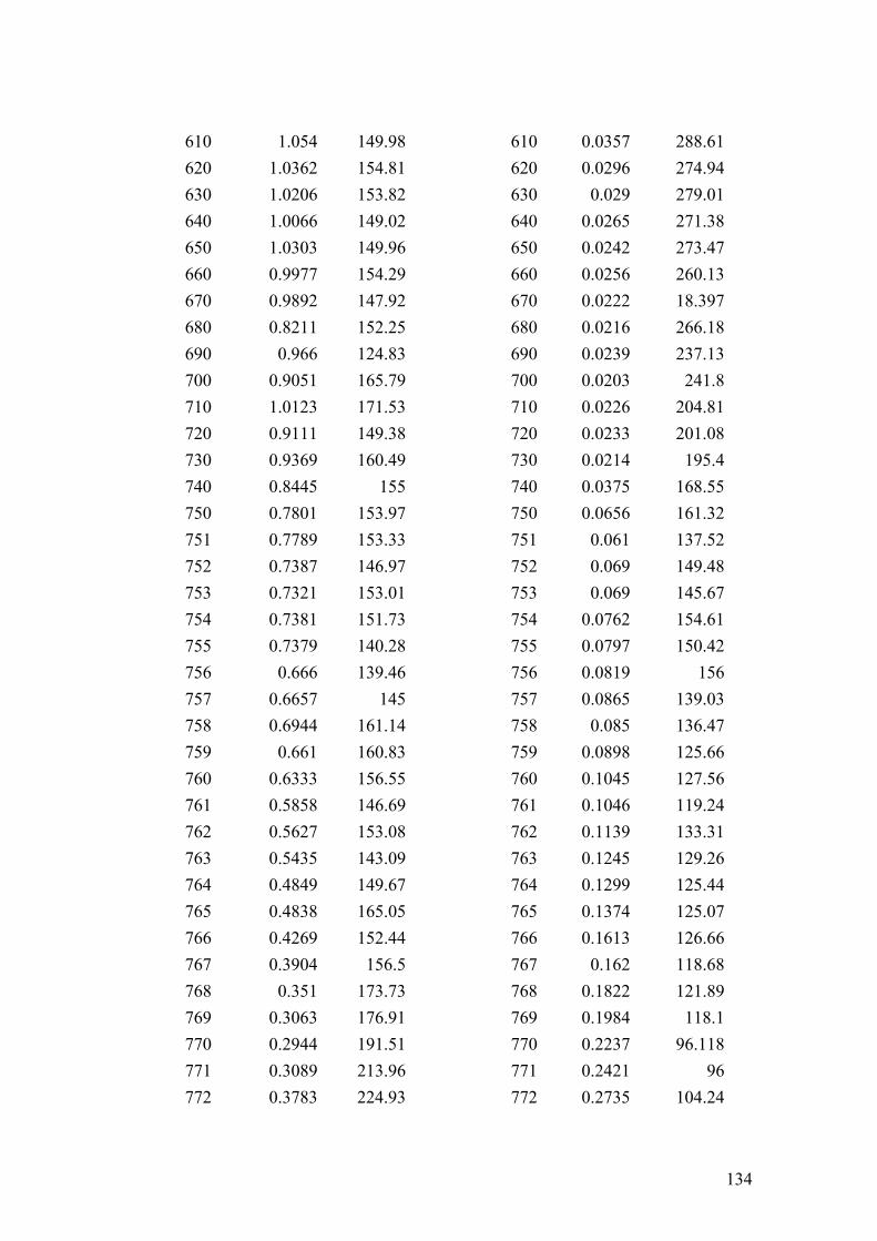
134
610 1.054 149.98 610 0.0357 288.61 620 1.0362 154.81 620 0.0296 274.94 630 1.0206 153.82 630 0.029 279.01 640 1.0066 149.02 640 0.0265 271.38 650 1.0303 149.96 650 0.0242 273.47 660 0.9977 154.29 660 0.0256 260.13 670 0.9892 147.92 670 0.0222 18.397 680 0.8211 152.25 680 0.0216 266.18 690 0.966 124.83 690 0.0239 237.13 700 0.9051 165.79 700 0.0203 241.8 710 1.0123 171.53 710 0.0226 204.81 720 0.9111 149.38 720 0.0233 201.08 730 0.9369 160.49 730 0.0214 195.4 740 0.8445 155 740 0.0375 168.55 750 0.7801 153.97 750 0.0656 161.32 751 0.7789 153.33 751 0.061 137.52 752 0.7387 146.97 752 0.069 149.48 753 0.7321 153.01 753 0.069 145.67 754 0.7381 151.73 754 0.0762 154.61 755 0.7379 140.28 755 0.0797 150.42 756 0.666 139.46 756 0.0819 156 757 0.6657 145 757 0.0865 139.03 758 0.6944 161.14 758 0.085 136.47 759 0.661 160.83 759 0.0898 125.66 760 0.6333 156.55 760 0.1045 127.56 761 0.5858 146.69 761 0.1046 119.24 762 0.5627 153.08 762 0.1139 133.31 763 0.5435 143.09 763 0.1245 129.26 764 0.4849 149.67 764 0.1299 125.44 765 0.4838 165.05 765 0.1374 125.07 766 0.4269 152.44 766 0.1613 126.66 767 0.3904 156.5 767 0.162 118.68 768 0.351 173.73 768 0.1822 121.89 769 0.3063 176.91 769 0.1984 118.1 770 0.2944 191.51 770 0.2237 96.118 771 0.3089 213.96 771 0.2421 96 772 0.3783 224.93 772 0.2735 104.24
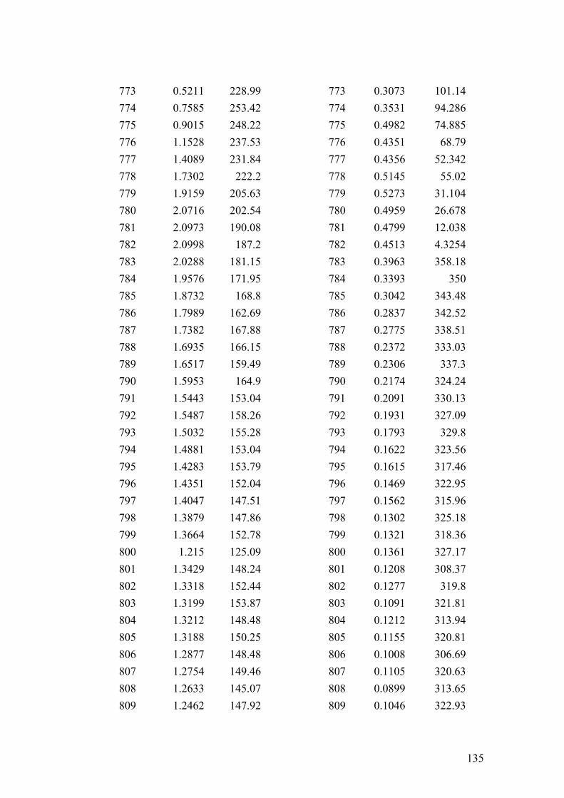
135
773 0.5211 228.99 773 0.3073 101.14 774 0.7585 253.42 774 0.3531 94.286 775 0.9015 248.22 775 0.4982 74.885 776 1.1528 237.53 776 0.4351 68.79 777 1.4089 231.84 777 0.4356 52.342 778 1.7302 222.2 778 0.5145 55.02 779 1.9159 205.63 779 0.5273 31.104 780 2.0716 202.54 780 0.4959 26.678 781 2.0973 190.08 781 0.4799 12.038 782 2.0998 187.2 782 0.4513 4.3254 783 2.0288 181.15 783 0.3963 358.18 784 1.9576 171.95 784 0.3393 350 785 1.8732 168.8 785 0.3042 343.48 786 1.7989 162.69 786 0.2837 342.52 787 1.7382 167.88 787 0.2775 338.51 788 1.6935 166.15 788 0.2372 333.03 789 1.6517 159.49 789 0.2306 337.3 790 1.5953 164.9 790 0.2174 324.24 791 1.5443 153.04 791 0.2091 330.13 792 1.5487 158.26 792 0.1931 327.09 793 1.5032 155.28 793 0.1793 329.8 794 1.4881 153.04 794 0.1622 323.56 795 1.4283 153.79 795 0.1615 317.46 796 1.4351 152.04 796 0.1469 322.95 797 1.4047 147.51 797 0.1562 315.96 798 1.3879 147.86 798 0.1302 325.18 799 1.3664 152.78 799 0.1321 318.36 800 1.215 125.09 800 0.1361 327.17 801 1.3429 148.24 801 0.1208 308.37 802 1.3318 152.44 802 0.1277 319.8 803 1.3199 153.87 803 0.1091 321.81 804 1.3212 148.48 804 0.1212 313.94 805 1.3188 150.25 805 0.1155 320.81 806 1.2877 148.48 806 0.1008 306.69 807 1.2754 149.46 807 0.1105 320.63 808 1.2633 145.07 808 0.0899 313.65 809 1.2462 147.92 809 0.1046 322.93
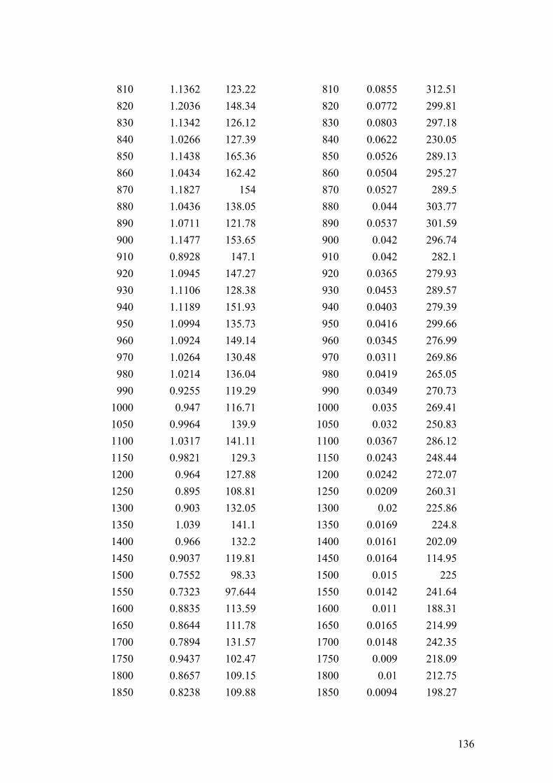
136
810 1.1362 123.22 810 0.0855 312.51 820 1.2036 148.34 820 0.0772 299.81 830 1.1342 126.12 830 0.0803 297.18 840 1.0266 127.39 840 0.0622 230.05 850 1.1438 165.36 850 0.0526 289.13 860 1.0434 162.42 860 0.0504 295.27 870 1.1827 154 870 0.0527 289.5 880 1.0436 138.05 880 0.044 303.77 890 1.0711 121.78 890 0.0537 301.59 900 1.1477 153.65 900 0.042 296.74 910 0.8928 147.1 910 0.042 282.1 920 1.0945 147.27 920 0.0365 279.93 930 1.1106 128.38 930 0.0453 289.57 940 1.1189 151.93 940 0.0403 279.39 950 1.0994 135.73 950 0.0416 299.66 960 1.0924 149.14 960 0.0345 276.99 970 1.0264 130.48 970 0.0311 269.86 980 1.0214 136.04 980 0.0419 265.05 990 0.9255 119.29 990 0.0349 270.73
1000 0.947 116.71 1000 0.035 269.41 1050 0.9964 139.9 1050 0.032 250.83 1100 1.0317 141.11 1100 0.0367 286.12 1150 0.9821 129.3 1150 0.0243 248.44 1200 0.964 127.88 1200 0.0242 272.07 1250 0.895 108.81 1250 0.0209 260.31 1300 0.903 132.05 1300 0.02 225.86 1350 1.039 141.1 1350 0.0169 224.8 1400 0.966 132.2 1400 0.0161 202.09 1450 0.9037 119.81 1450 0.0164 114.95 1500 0.7552 98.33 1500 0.015 225 1550 0.7323 97.644 1550 0.0142 241.64 1600 0.8835 113.59 1600 0.011 188.31 1650 0.8644 111.78 1650 0.0165 214.99 1700 0.7894 131.57 1700 0.0148 242.35 1750 0.9437 102.47 1750 0.009 218.09 1800 0.8657 109.15 1800 0.01 212.75 1850 0.8238 109.88 1850 0.0094 198.27

137
1900 0.7782 103.37 1900 0.0085 193.91 1950 0.7617 88.129 1950 0.0061 324.9 2000 0.7738 97.278 2000 0.0092 108.78 2010 0.7829 88.918 2010 0.0091 24.597 2020 0.7647 99.085 2020 0.0093 108.02 2030 0.8231 118.7 2030 0.0123 96.515 2040 0.6362 105.55 2040 0.0199 85.714 2041 0.7133 102.01 2041 0.0238 89.918 2042 0.7417 111.56 2042 0.0198 90.041 2043 0.6434 118.7 2043 0.0222 90.768 2044 0.676 96.825 2044 0.0229 92.701 2045 0.6955 110.54 2045 0.0268 85.913 2046 0.658 96.759 2046 0.0322 71.837 2047 0.6426 96.475 2047 0.0303 73.072 2048 0.6129 100.95 2048 0.0377 70.588 2049 0.6057 116.73 2049 0.0425 70.109 2050 0.5441 93.496 2050 0.057 69.136 2051 0.5111 85.246 2051 0.0567 80.109 2052 0.3745 112.29 2052 0.0802 74.188 2053 0.3305 156.31 2053 0.098 63.76 2054 0.9922 130.97 2054 0.1672 65.041 2055 0.7007 135.51 2055 0.3299 20.683 2056 2.6229 169.81 2056 0.1627 348.74 2057 2.0399 95.473 2057 0.2933 350.43 2058 1.2033 87.686 2058 0.2563 283.76 2059 1.1479 92.461 2059 0.1549 268.12 2060 1.2029 114.1 2060 0.092 265.92 2061 1.0229 85.014 2061 0.086 276.96 2062 1.1166 89.796 2062 0.0859 268.32 2063 0.9589 110.88 2063 0.0552 240.7 2064 0.8515 100.69 2064 0.0454 257.56 2065 1.0106 87.243 2065 0.0453 258.39 2066 0.931 95.872 2066 0.037 251.94 2067 0.9314 96.326 2067 0.0434 242.45 2068 1.0094 84.182 2068 0.0444 238.34 2069 0.8058 83.039 2069 0.0357 256.72 2070 0.9516 85.714 2070 0.0336 234.07

138
2071 0.8919 94.526 2071 0.0259 235.98 2072 0.9999 112.12 2072 0.0267 224.18 2073 0.8492 97.386 2073 0.0234 243.29 2074 0.8873 100.14 2074 0.0224 224.48 2075 0.8708 95.872 2075 0.0381 304.11 2076 0.9663 109.52 2076 0.0213 226.04 2077 0.9755 113.09 2077 0.0241 235.03 2078 0.9667 113.42 2078 0.0225 238.19 2079 0.9613 91.803 2079 0.0203 239.34 2080 0.7441 97.79 2080 0.0174 240.65 2090 0.7486 100.27 2090 0.0202 241.5 2100 0.8299 93.724 2100 0.0151 209.42 2150 0.8343 102.26 2150 0.0089 188.03 2200 0.7706 92.176 2200 0.008 336.93 2250 0.7918 93.527 2250 0.0065 346.34 2300 0.7447 79.42 2300 0.0093 197.65 2350 0.6889 76.034 2350 0.0047 114.87 2400 0.7394 85.493 2400 0.0045 187.51 2450 0.7819 74.755 2450 0.0062 167.86 2500 0.6842 81.84 2500 0.0061 151.55 2550 0.6511 82.4 2550 0.0037 171.99 2600 0.709 75.85 2600 0.0052 271.41 2650 0.7345 72.12 2650 0.0052 108.18 2700 0.69 75.271 2700 0.0043 154.06 2750 0.6752 63.905 2750 0.0044 156.3 2800 0.6798 66.661 2800 0.0039 93.705 2850 0.6923 63.586 2850 0.0043 174.15 2900 0.7299 81.134 2900 0.0029 120.64 2950 0.6325 66.948 2950 0.0043 72.623 3000 0.6551 64.392 3000 0.0048 137.68 3050 0.6454 60.508 3050 0.0038 147.53

139
APPENDIX C
C2DM Conversion of continuous LTI systems to discrete-time

140
C2DM Conversion of continuous LTI systems to discrete-time. [Ad,Bd,Cd,Dd] = C2DM(A,B,C,D,Ts,'method') converts the continuous- time state-space system (A,B,C,D) to discrete time using 'method': 'zoh' Convert to discrete time assuming a zero order hold on the inputs. 'foh' Convert to discrete time assuming a first order hold on the inputs. 'tustin' Convert to discrete time using the bilinear (Tustin) approximation to the derivative. 'prewarp' Convert to discrete time using the bilinear (Tustin) approximation with frequency prewarping. Specify the critical frequency with an additional argument, i.e. C2DM(A,B,C,D,Ts,'prewarp',Wc) 'matched' Convert the SISO system to discrete time using the matched pole-zero method. [NUMd,DENd] = C2DM(NUM,DEN,Ts,'method') converts the continuous- time polynomial transfer function G(s) = NUM(s)/DEN(s) to discrete time, G(z) = NUMd(z)/DENd(z), using 'method'.

141
APPENDIX D
Equation Derivation

142
1. Equation 3.16
θθθ cos)(cos)( 21220 lFlFIM LL −−−==⋅⋅
∑
is derived from equation 3.7 ; 3.8 and 3.15 :
θsin)( 201 lxx L −−=
Equation 3.7
θsin)( 202 lxx L −+=
Equation 3.8
210 FFxmF +==⋅⋅
∑
Equation 3.15
2. Equation 3.20
mF
mF 21
0 +=⋅⋅
χ
is derived from equation 3.15
210 FFxmF +==⋅⋅
∑
3. Equation 3.21
20
100
21
0
22 )2
(1)2
(1)()(FlL
IFlL
IIlF
IlF LL
−+−−=−
−−
=⋅⋅
θ
is derived from equation 3.16
θθθ cos)(cos)( 21220 lFlFIM LL −−−==⋅⋅
∑

143
4. Equation 3.22
θ)( 2201 lxX L −−=
is derived from equation 3.9
θsin)( 2201 lxX L −−=
5. Equation 3.23
θ)( 2202 lxX L −+=
is derived from equation 3.10
θsin)( 2202 lxX L −+=
6. Equation 3.24
⎥⎦
⎤⎢⎣
⎡
⎥⎥⎥⎥⎥
⎦
⎤
⎢⎢⎢⎢⎢
⎣
⎡
−
+
⎥⎥⎥⎥⎥
⎦
⎤
⎢⎢⎢⎢⎢
⎣
⎡
⎥⎥⎥⎥
⎦
⎤
⎢⎢⎢⎢
⎣
⎡
=
⎥⎥⎥⎥⎥
⎦
⎤
⎢⎢⎢⎢⎢
⎣
⎡
−−
⋅⋅⋅
⋅2
1
)(1
)(1
110
.0
0
..0
.
2020
00
00
0000100000000010
FFx
x
xx
lIlI
mm
LLθθ
θθ
is derived from equations 3.20 and 3.21
mF
mF 21
0 +=⋅⋅
χ
Equation 3.20
20
100
21
0
22 )2
(1)2
(1)()(FlL
IFlL
IIlF
IlF LL
−+−−=−
−−
=⋅⋅
θ
Equation 3.21
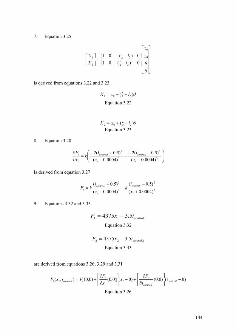
144
7. Equation 3.25
⎥⎥⎥⎥⎥
⎦
⎤
⎢⎢⎢⎢⎢
⎣
⎡
⎥⎦
⎤⎢⎣
⎡−−−
=⎥⎦
⎤⎢⎣
⎡
⋅
θθ
0
.0
22
22
2
1
0)(010)(01 x
x
ll
XX
l
l
is derived from equations 3.22 and 3.23
θ)( 2201 lxX L −−=
Equation 3.22
θ)( 2202 lxX L −+=
Equation 3.23
8. Equation 3.28
⎟⎟⎠
⎞⎜⎜⎝
⎛+
−−−
−+−
=∂∂
3
2
3
2
)0004.0()5.0(2
)0004.0()5.0(2
i
controli
i
controli
i
i
xi
xi
kxF
Is derived from equation 3.27
2
2
2
2
)0004.0()5.0(
)0004.0()5.0(
+
−−
−
+=
i
control
i
controli x
ik
xi
kF ii
9. Equations 3.32 and 3.33
111 5.34375 controlixF +=
Equation 3.32
222 5.34375 controlixF +=
Equation 3.33
are derived from equations 3.26, 3.29 and 3.31
)0()0,0()0()0,0()0,0(),( −⎥⎦
⎤⎢⎣
⎡∂∂
+−⎥⎦
⎤⎢⎣
⎡∂∂
+= controlicontroli
ii
i
iicontroliii i
iF
xxF
FixF
Equation 3.26

145
4375)0,0(
=∂∂
i
i
xF
Equation 3.29
5.3)0,0(
=∂∂
controli
i
iF
Equation 3.31
10. Equation 3.34
1201 5.3)(43754375 controlL ilxF +−−= θ
is derived from equations 3.7 and 3.32
θsin)( 201 lxx L −−=
Equation 3.7
111 5.34375 controlixF += Equation 3.32
11. Equation 3.35
2202 5.3)(43754375 controlL ilxF +−+= θ
is derived from equations 3.8 and 3.33
θsin)( 202 lxx L −+=
Equation 3.8
222 5.34375 controlixF +=
Equation 3.33

146
12. Equation 3.36
milx
milx
x controlL
controlL
2201200
.. 5.3)(437543755.3)(43754375 +−++
+−−=
θθ
mi
mi
xm
x controlcontrol 2100
.. 5.35.38750++=
is derived from equations 3.20, 3.34 and 3.35
mF
mF 21
0 +=⋅⋅
χ
Equation 3.20
1201 5.3)(43754375 controlL ilxF +−−= θ
Equation 3.34
2202 5.3)(43754375 controlL ilxF +−+= θ
Equation 3.35 13. Equation 3.37
20
21
0
2
0
22 )(
5.3)(
5.3)(
8750 control
L
control
LL
iI
li
Il
Il θθθ
θ−
+−
−−
=⋅⋅
is derived from equations 3.21 ; 3.34 and 3.35
20
100
21
0
22 )2
(1)2
(1)()(FlL
IFlL
IIlF
IlF LL
−+−−=−
−−
=⋅⋅
θ
Equation 3.21
1201 5.3)(43754375 controlL ilxF +−−= θ
Equation 3.34

147
2202 5.3)(43754375 controlL ilxF +−+= θ
Equation 3.35
14. Equation 3.38
⎥⎦
⎤⎢⎣
⎡
⎥⎥⎥⎥⎥
⎦
⎤
⎢⎢⎢⎢⎢
⎣
⎡
−−−
+
⎥⎥⎥⎥⎥
⎦
⎤
⎢⎢⎢⎢⎢
⎣
⎡
⎥⎥⎥⎥⎥
⎦
⎤
⎢⎢⎢⎢⎢
⎣
⎡
=
⎥⎥⎥⎥⎥
⎦
⎤
⎢⎢⎢⎢⎢
⎣
⎡
−⋅⋅
⋅2
1
25.3
25.3
5.35.30
.0
)(8750
87500
..0
.
)()(00
00
00010000000010
000
22
control
control
LI
LI
mm
Il
m
ii
ll
x
x
xx
L
θθ
θθ
&
is derived from equations 3.36 and 3.37
mi
mix
mx controlcontrol 21
00
.. 5.35.38750++=
Equation 3.36
20
21
0
2
0
22 )(
5.3)(
5.3)(
8750 control
L
control
LL
iI
li
Il
Il θθθ
θ−
+−
−−
=⋅⋅
Equation 3.37
15. Equation 3.39
⎥⎥⎥⎥⎥
⎦
⎤
⎢⎢⎢⎢⎢
⎣
⎡
⎥⎦
⎤⎢⎣
⎡−−−
=⎥⎦
⎤⎢⎣
⎡
⋅
θθ
0
.0
22
22
2
1
0)(010)(01 x
x
ll
XX
L
L
is derived from equations 3.22 and 3.23
θ)( 2201 lxX L −−=
Equation 3.22

148
θ)( 2202 lxX L −+=
Equation 3.23 16. Equation 3.45
rL
L
sense
sense xll
VV
⎥⎦
⎤⎢⎣
⎡−−−
=⎥⎦
⎤⎢⎣
⎡0)(010)(01
500022
22
2
1
is derived from equations 3.22, 3.23 and 3.43
θ)( 2201 lxX L −−=
Equation 3.22
θ)( 2202 lxX L −+=
Equation 3.23
5000)0(
=∂
∂
i
sensei
XV
Equation 3.43
17. Equation 3.47
rL
L
sense
sense xll
VV
⎥⎦
⎤⎢⎣
⎡−−−
=⎥⎦
⎤⎢⎣
⎡000)(01000)(01
500022
22
2
1
is derived from equations 3.36, 3.37 and 3.46
mi
mi
xm
x controlcontrol 2100
.. 5.35.38750++=
Equation 3.36

149
20
21
0
2
0
22 )(
5.3)(
5.3)(
8750 control
L
control
LL
iI
li
Il
Il θθθ
θ−
+−
−−
=⋅⋅
Equation 3.37
⎥⎦
⎤⎢⎣
⎡
⎥⎥⎥⎥⎥⎥⎥⎥
⎦
⎤
⎢⎢⎢⎢⎢⎢⎢⎢
⎣
⎡
+
⎥⎥⎥⎥⎥⎥⎥⎥
⎦
⎤
⎢⎢⎢⎢⎢⎢⎢⎢
⎣
⎡
−−−−=
−
−
−
−
×
×
×−
×−
2
1
102.225.0
102.225.0
102.21
102.21
25.3
25.3
22
5.35.38750
.
4
4
4
4
00
0000000000
0000000000
)()(0)(875000
001000000
000010
control
controlrL
IL
Io
L
mmm
rVV
xllI
lx
Equation 3.46
18. Equation 3.48
⎥⎦
⎤⎢⎣
⎡≡
2
1
aa
a
is derived from equations 3.22, 3.23 and 3.43
θ)( 2201 lxX L −−=
Equation 3.22
θ)( 2202 lxX L −+=
Equation 3.23
5000)0(
=∂
∂
i
sensei
XV
Equation 3.43
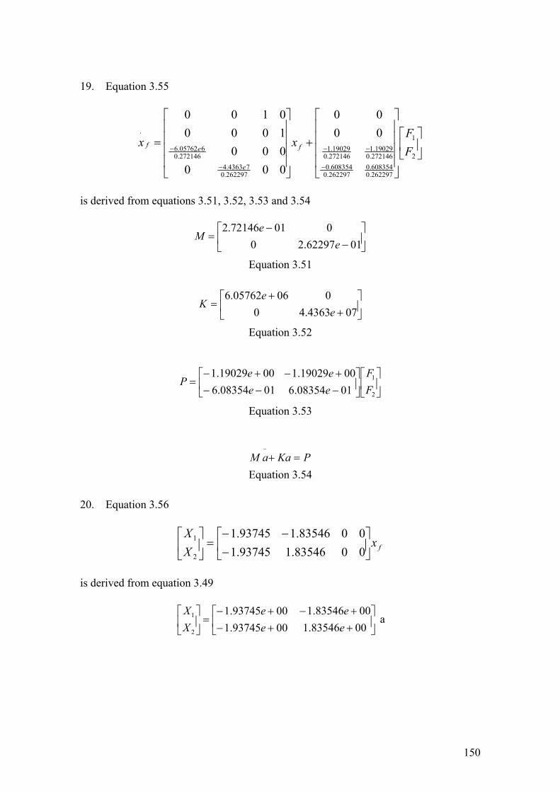
150
19. Equation 3.55
⎥⎦
⎤⎢⎣
⎡
⎥⎥⎥⎥
⎦
⎤
⎢⎢⎢⎢
⎣
⎡
+
⎥⎥⎥⎥
⎦
⎤
⎢⎢⎢⎢
⎣
⎡
=
−
−−
−
−
⋅
2
1
262297.0608354.0
262297.0608354.0
272146.019029.1
272146.019029.1
262297.074363.4
272146.0605762.6
0000
00000010000100
FF
xx f
e
ef
is derived from equations 3.51, 3.52, 3.53 and 3.54
⎢⎣
⎡ −=
00172146.2 e
M ⎥⎦
⎤− 0162297.2
0e
Equation 3.51
⎢⎣
⎡ +=
00605762.6 e
K ⎥⎦
⎤+ 074363.4
0e
Equation 3.52
⎢⎣
⎡−−+−
=0108354.60019029.1
ee
P ⎥⎦
⎤⎢⎣
⎡⎥⎦
⎤−+−
2
1
0108354.60019029.1
FF
ee
Equation 3.53
PKaaM =+⋅⋅
Equation 3.54 20. Equation 3.56
fxXX
⎥⎦
⎤⎢⎣
⎡−
−−=⎥
⎦
⎤⎢⎣
⎡0083546.193745.10083546.193745.1
2
1
is derived from equation 3.49
⎢⎣
⎡+−+−
=⎥⎦
⎤⎢⎣
⎡0093745.10093745.1
2
1
ee
XX
⎥⎦
⎤++−0083546.10083546.1
ee
a

151
21. Equation 3.57
⎥⎦
⎤⎢⎣
⎡
⎥⎥⎥⎥⎥⎥⎥⎥⎥⎥⎥
⎦
⎤
⎢⎢⎢⎢⎢⎢⎢⎢⎢⎢⎢
⎣
⎡
−−−
−+
⎥⎥⎥⎥⎥⎥⎥⎥⎥⎥⎥
⎦
⎤
⎢⎢⎢⎢⎢⎢⎢⎢⎢⎢⎢
⎣
⎡
−−
=⋅
2
1.
3193.23193.23737.43737.400005669.695669.6900
8037.38037.300
0086913.1000000007226.20000100000000100000000000000000010000000000000000010
FF
x
ee
x totaltotal
is derived from equations 3.50, 3.51, 3.52 and 3.53
⎢⎣
⎡+−+−
=⎥⎦
⎤⎢⎣
⎡0019029.10019029.1
2
1
ee
xx
⎥⎦
⎤−−−−
0108354.60108354.6
ee
a
Equation 3.50
⎢⎣
⎡ −=
00172146.2 e
M ⎥⎦
⎤− 0162297.2
0e
Equation 3.51
⎢⎣
⎡ +=
00605762.6 e
K ⎥⎦
⎤+ 074363.4
0e
Equation 3.52
⎢⎣
⎡−−+−
=0108354.60019029.1
ee
P ⎥⎦
⎤⎢⎣
⎡⎥⎦
⎤−+−
2
1
0108354.60019029.1
FF
ee
Equation 3.53

152
APPENDIX E Fuzzy Theory

153
Fuzzy Theory Fuzzy Set
Fuzzy logic is designed for situations where information is inexact and the traditional
binary logic based on “true” (or “1”) and “false” (or “0”) are not possible. Fuzzy logic is
a form of logic in which variables can have degrees of truth or falsehood. Fuzzy logic
starts with the concept of a fuzzy set. Fuzzy set consists of elements with only a partial
degree of membership.
A fuzzy set F in a universe of discourse U is characterised by a membership function µ
which takes values in the interval [0,1] namely, µF: U → [0,1].
Membership Function (MF)
A membership function (MF) is a curve that defines how to map every point in the input
to a membership value or degree of membership between 0 and 1. The input is referred
to as the universe of discourse. Figure 1 shows some typical membership functions
(Passino and Yurkovich 1998). The typical membership functions may include
triangular membership function, trapezoidal membership function, a simple Gaussian
membership function, a two-sided composite of two different Gaussian curves,
generalised bell shape membership function, sigmoidal membership functions, a
singleton membership function, etc (A Zadeh 1995).

154
Figure1 Some typical membership functions
Source : (Passino and Yurkovich 1998; Mukaidono 2001)
The triangular membership function is commonly used due to its simplicity. Because of
the smoothness and concise notation of the Gaussian membership function, it is also
often used for specifying fuzzy sets. The mathematical descriptions of the triangular and
Gaussian membership functions are provided in Tables 1 and 2 (Reznik 1997; Passino
and Yurkovich 1998).
Additional concepts related to membership functions and fuzzy sets such as support of a
fuzzy set, α-cut, height of a fuzzy set or membership function, normal fuzzy sets, convex
fuzzy sets, extension principle can be found in (Reznik 1997; Passino and Yurkovich
1998).
Triangular Membership Function
Left { } otherwisecuif
uL
ucL
L
L
≤
⎩⎨⎧
+= −
ω
μ5.0
1,0max1
)(
Centres{ }{ } otherwise
cuifu
uc
cuC ≤
⎩⎨⎧
++
=−
−
ω
ωμ5.0
5.0
1,0max1,0max
)(
Right { }
otherwisecuif
uRcu
R R
R ≤
⎩⎨⎧ +
=−
11,0max)( 5.0 ωμ
Table 1 Mathematical characterisation of triangular membership function Source: (Reznik 1997; Passino and Yurkovich 1998)
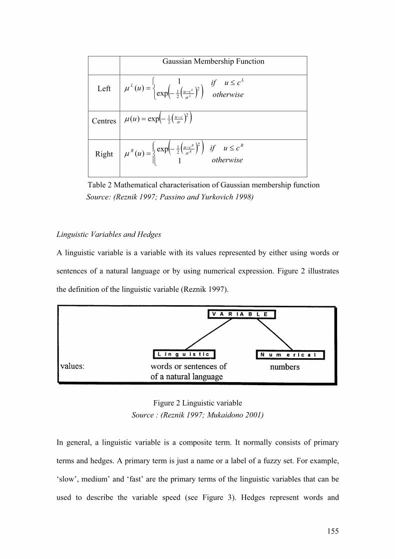
155
Gaussian Membership Function
Left ( )( ) otherwisecuif
uL
cuL
L
L
≤
⎩⎨⎧
−= − 2
21exp1
)(σ
μ
Centres ( )( )221exp)( σμ cuu −−=
Right ( )( )otherwise
cuifu
RcuR R
R ≤
⎪⎩
⎪⎨⎧ −=
−
1exp)(
2
21
σμ
Table 2 Mathematical characterisation of Gaussian membership function Source: (Reznik 1997; Passino and Yurkovich 1998)
Linguistic Variables and Hedges
A linguistic variable is a variable with its values represented by either using words or
sentences of a natural language or by using numerical expression. Figure 2 illustrates
the definition of the linguistic variable (Reznik 1997).
Figure 2 Linguistic variable Source : (Reznik 1997; Mukaidono 2001)
In general, a linguistic variable is a composite term. It normally consists of primary
terms and hedges. A primary term is just a name or a label of a fuzzy set. For example,
‘slow’, medium’ and ‘fast’ are the primary terms of the linguistic variables that can be
used to describe the variable speed (see Figure 3). Hedges represent words and

156
expression of the natural language and a vocabulary of the natural language. Typical
hedges are ‘very’, ‘most’, ‘rather’, ‘slightly’, ‘more or less’, etc. Some widely used
hedges and their meanings are shown in Table 3 (Reznik 1997; Mukaidono 2001).
Hedge Meaning About, around, near, roughly Approximate a scalar Above, more than Restrict a fuzzy region Almost, definitely, positively Contrast intensification Below, less than Restrict a fuzzy region Vicinity of Approximate broadly Generally, usually Contrast diffusion Neighbouring, close to Approximately narrowly Not Negation or complement Quite, rather, somewhat Dilute a fuzzy region Very, extremely Intensify a fuzzy region
Table 3 Some widely used hedges Source: (Reznik 1997; Mukaidono 2001)
Figure 3 Membership functions for linguistic values Source: (Reznik 1997; Passino and Yurkovich 1998)

157
Figure 4 shows the application of different hedges to describe ‘medium’ speed.
0 5 10 15 20 25 30 0
0.1
0.2
0.3
0.4
0.5
0.6
0.7
0.8
0.9
1 average
very average
close to, neibouring average
about, around, near, roughly average
in the vicinity of average
speed
Figure 4 Application of different hedges Source: (Reznik 1997; Mukaidono 2001)
Operations on Fuzzy sets
Fuzzy Complement:
The complement of a fuzzy set A has a membership function which is pointwise defined
for all u ∈ U by:
μA( u ) = 1 - μA( u ).
This corresponds to the logic NOT operation.
Fuzzy Intersection:
The intersection of two fuzzy sets C= A ∩ B has the membership function:
μA ∩ B (u ) = μA(u) t μB(u) ≤ Min (μA(u) , μB(u) )
where t is a triangular norm (or measure) defined as follows:
The t norm or triangular norm is a two place function from [0,1] * [0,1] to [0,1], i.e. t:
[0,1] * [0,1] → [0,1] which is non-decreasing in each element x t w ≤ y t z if x ≤ y,

158
w ≤ z. It is commutative, associative and satisfies boundary conditions x t 0 = 0, and x t
1 = x; for any x,y,z,w ∈ [0,1].
Figure 5 displays two different ways for calculating t-norm operations. One method
uses minimum operation and the other method uses product operation.
Figure 5 Two different ways (minimum and product) for calculating t-norm operations Source: (Reznik 1997; Passino and Yurkovich 1998)
Fuzzy Union
The union (or disjunction) of two fuzzy sets C = A ∪ B has the membership function:
μA ∪ B (u ) = μA(u) s μB(u) ≥ Max ( μA(u) , μB(u) )
where s is a triangular co-norm (or measure, or s -norm) defined as follows:
The s norm or triangular co-norm is a two place function from [0,1] * [0,1] to [0,1], i.e.
s: [0,1] * [0,1] → [0,1] which is non-decreasing in each element, commutative,
associative and satisfies boundary conditions x s 0 = x, and x s 1 = 1; for all x ∈ [0,1].
Some classes of fuzzy set unions and intersections are shown in Table 4.

159
SOME CLASSES OF FUZZY SET UNIONS AND INTERSECTIONS
Reference Fuzzy Unions Fuzzy Intersections Range of Parameter ___________________________________________________________________ Max (a,b) Min (a,b) ____________________________________________________________________ a + b - ab ab ____________________________________________________________________ Schweizer & 1 - max[0, (1 - a) -p + (1 +b) -p -1)] 1/p max(0,a-p +b-p -1)-1/p p ∈ (- ∞,∞) Sklar [1961] ____________________________________________________________________ Hamacher (a +b - (2 - g) ab)/(1 - (1 - g)ab) ab/(g+(1-g)(a+b-ab)) g ∈ (0, ∞ )
[1978] ______________________________________________________________________ Frank [1979] 1 -- logs [1+ (s1-a -1) (s1-b -1)/s -1] logs [1+(sa-1)(sb-1)/s-1] s ∈ (0,∞ )
______________________________________________________________________ Yager [1980] Min[ 1, (aw+bw)1/w] 1-Min[1,(1-a)w+(1-b)w)1/w] w ∈ (0, ∞ )
_____________________________________________________________________ Dubois & a +b - ab - min(a,b,1 - α)
Prade [1980] __________________ ab/max(a,b,α) α ∈ (0,1)
max(1-a,1-b,α)
______________________________________________________________________ Dombi [1982]
1 1
______________________ ___________________ λ ∈ (0,∞)
1+[(1/a-1)-λ +(1/b -1) -λ]-1/λ 1+[(1/a-1)λ +(1/b-1)λ]1/λ
Table 4 Some classes of fuzzy set unions and intersections Source: (Reznik 1997; Passino and Yurkovich 1998)

160
The Rule Base
Most of the fuzzy logic applications involve fuzzy rules construction and processing.
Fuzzy rules are used to describe qualitative dependencies between two or more
variables in linguistic terms. Fuzzy rules processing or reasoning provides a mechanism
for using fuzzy rules to compute the response to a given fuzzy input. The If-Then rule
statements are used to formulate the conditional statements that represent fuzzy logic.
The general form of the linguistic rules is:
If premise Then consequent
The premises are sometimes called antecedents, they are associated with the fuzzy
inputs and are put on the left-hand-side of the rules, while the consequents which are
sometimes called different names such as conclusions or actions are associated with the
fuzzy outputs and are put on the right-hand-side of the rules (Reznik 1997; Passino and
Yurkovich 1998). For example one of the rules developed for the fuzzy logic controller
for the magnetic bearing system can be represented as:
If error is negative big and change-in-error is negative big Then force is negative big.
Some important properties for a set of rules are (Reznik 1997; Passino and Yurkovich
1998):
Completeness
A set of if-then rules is complete if any combination of input values results in an
appropriate output value.
Consistency
A set of if-then rules is inconsistent if there are two rules with the same rules-
antecedent but different rule-consequent.

161
Continuity
A set of if-then rules is continuous if it does not have neighbouring rules with
output fuzzy sets that have empty intersections.
Fuzzy Cartesian Product
The intersection and union described previously are both defined for fuzzy sets that lie
on the same universe of discourse. The fuzzy Cartesian product is used to quantify
operations on many universes of discourse. If A1, …, An are fuzzy sets in the universes
of discourse U1, …, Un then the Cartesian product of A1, …, An is a fuzzy set in the
product space U1*…* Un with the membership function:
μA1*…*An (u1,…,un ) = μA1(u1) t μA2(u2) t …t μAn(un)
The t norm used in the Cartesian product represents the “ands” used in the rule
antecedent as each of the terms in an antecedent comes from a different universe of
discourse (Reznik 1997; Passino and Yurkovich 1998).
Fuzzy Quantification of Rules: Fuzzy Implications Fuzzy implication is used to quantify the linguistic elements in the antecedent and the
consequent of the linguistic If-Then rule with fuzzy sets.
Fuzzification
Fuzzification is the process of converting numeric inputs into fuzzy sets. These fuzzy
sets are used to quantify the information in the rule base. The inference mechanism
operates on the fuzzy sets in the rule base to produce fuzzy sets.

162
The Inference Mechanism
The inference mechanism is used to produce fuzzy sets representing the conclusions that
it reaches using the current inputs and the rule base. The inference mechanism has two
basic tasks. The first task is called matching and the second is called inference. In the
first task, the extent to which a rule is relevant to the current situation as characterised
by the inputs is determined. The antecedents of all the rules are compared to the
controller inputs in order to determine which rules apply to the current situation. The
“matching” process involves determining the certainty that each rule applies, and
recommending certain rules to be applied to the current situation. Matching involves
two basic steps. The first step of the matching combines the fuzzy sets from
fuzzification with the fuzzy sets used in each of the terms in the antecedents of the rule.
The second step of matching determines which rules are on. Membership values
represent the certainty of an antecedent of a rule is determined in that particular step. In
the inference step, conclusions are drawn from the current inputs and the information in
the rule-base. There are two standard alternatives in this step. One method uses the
implied fuzzy sets. The implied fuzzy set specifies the certainty level that the output
should be a specific crisp output with the output universe of discourse, taking into
consideration one rule at a time. Another inference method computes the overall
implied fuzzy set considering all the rules in the rule base at the same time (A Zadeh
1995; Passino and Yurkovich 1998).

163
Defuzzification
The defuzzification process converts the fuzzy set quantifications of the conclusions
obtained in the inference step to a numeric value that can be applied to the plant.
There are many defuzzification methods. Each method produces a single output based
on either the implied fuzzy sets or the overall implied fuzzy set.
Drawing on (A Zadeh 1995; Reznik 1997), some of the defuzzification methods are
listed below:
o Centre of Area / Gravity (CoA)
o Centre average
o Centre of Largest Area (CLA)
o First of Maxima (FoM) /Last of Maxima
o Middle of Maxima (MoM)
o Mean of maxima
o Height of defuzzification (HM)
Comparison of different defuzzification procedures uses the following four
characteristics:
• Continuity
A small change in an input of a fuzzy controller should not result in a large change in
the output.
• Disambiguity
A deffuzzification method should work in any situation. The centre of largest area
method does not allow a choice when there are two equal areas.

164
• Plausibility
A procedure produces a defuzzified output that lies approximately in the middle of
the support of the resulting membership function and has a high degree of
membership.
• Computational Complexity
This is important in practical applications. It depends on the shape of the output
membership function and the max-min composition or the scaled composition.
Table 5 compares a few different defuzzification methods using the above characteristic
descriptions.
CoA MoM FoM HM CLA
Continuity Yes No No Yes No
Disambiguity Yes Yes Yes Yes No
Plausibility Yes No* No Yes Yes
Computational
Complexity
Bad Good Good Good Bad
Table 5 Comparison of deffuzzification methods Source: (Reznik 1997; Passino and Yurkovich 1998)
CoA= Centre of Area
MoM=Middle of Maxima
FoM=First of Maxima
HM=Height and Mean of maxima
CLA=Centre of Largest Area
No*=only in the case of scaled inference

165
The fuzzy system described above is either called a standard fuzzy system or referred to
as the Mamdani method. Alternatively, another method of fuzzy processing is defined
as a functional fuzzy system which is referred to as the Sugeno method. In the Sugeno
method, the antecedent part of the rule is similar to that of the Mamdani method.
However, the consequent parts of the rules are different. The consequent part uses a
mathematical function of the input variables instead of a linguistic term with an
associate membership function (Passino and Yurkovich 1998).
Table 6 shows some similarities and differences between these two methods.
Mamdani Takagi-Sugeno Similarity The antecedent parts of the rules are the same.
Difference The consequent parts are fuzzy sets.
The consequent parts are singletons (single spikes) or mathematical functions of them. It is more effective computationally. It is more convenient in mathematical and system analysis.
Advantages It is very understandable by human experts. It is simpler to formulate rules. This method was proposed earlier and commonly used. It guarantees continuity of the
output surface. Table 6 Comparison of Mamdani and Takagi-Sugeno Methods
Sources: (Reznik 1997; Passino and Yurkovich 1998; Mukaidono 2001) Figure 6 shows an example illustrating the fuzzy processing described in this section using the Mamdani and Sugeno methods (Reznik 1997).

166
-30 -20 -10 0 10 20 3000.10.20.30.40.50.60.70.80.91
pressure
NBig NSmall Zero PSmall PBig
input crisp
Input crisp= -22
Inputfuzzy =(NBig,0.8) (NSm,0.05)
0 5 10 15 20 25 3000.10.20.30.40.50.60.70.80.91
temperature
low medium high
crisp input
crisp input = 22
fuzzy input =(High, 0.6),(Med., 0.1)
Crisp inputsP=-22 t = 22
Fuzzy inputs
Calculation of the degree of applicabilityfor each rule
β = A 1 (x 1) t A 2 (x 2) t ... t A n (x n)
Degrees ofapplicability
0 5 10 15 20 2500.10.20.30.40.50.60.70.80.9
1 Short- clipped- scaled
time
if pressure is Neg Big and temperature is high then time is short ♣ - firedif pressure is Neg Small and temperature is high then time is short ♣ - firedif pressure is Zero and temperature is low then time is averageif pressure is Pos Small and temperature is medium then time is longif pressure is Pos Big and temperature is medium then time is long
Rulestable
Fuzzy outputsMamdani method:clipping or scalingoutput fuzzy sets
Sugeno method:Math.function calculation
f = a 0 + a 1 × x 1 + a 2 × x 2 + . . . + a n × x n
of each rule
Union (s-norm) of all rules outputs
Fuzzy output Figure 6 An example of fuzzy processing using Mamdani and Takagi-Sugeno methods
Source: (Reznik 1997; Passino and Yurkovich 1998)